Operational Metrics to Assess Performances of a Prognosis Function. Application to Lubricant of a Turbofan Engine Over- Consumption Prognosis. Ouadie HMAD 1 , Jean-Rémi MASSE 2 , Edith GRALL-MAËS 3 , Pierre BEAUSEROY 4 and Agnès MATHEVET 5 1,5 Safran Engineering Services, Moissy Cramayel, 77550, FRANCE [email protected][email protected]2 Safran Snecma, Moissy Cramayel, 77550, FRANCE [email protected]1,3,4 UMR STMR – LM2S – ICD – Université de Technologie de Troyes, Troyes, 10000, FRANCE [email protected][email protected]ABSTRACT In the aeronautical field, one of the major concerns is the availability of systems. To ensure availability, Prognosis and Health Management algorithms are developed. The aim of these algorithms is twofold. The first one is to detect and locate degradation premise of “no go” condition occurrence. The second one is to predict the health state of the system at a given time horizon. Before introducing PHM algorithms in operation, it is necessary to assess their performances. This is accomplished thank to a “maturation” phase. This phase consists in defining the performance metrics from an operational relevance point of view, in estimating this performance indicator and finally in proposing improvements to meet the airline companies requirements. We consider that the maturation of the detection function has already been completed and that we are interested in the maturation of the prognosis function. This paper deals with the performance assessment of a prognosis function using two operational metrics. A performance estimation procedure is developed. It is applied to the prognosis of turbofan engine lubricant over-consumption. The considered prognosis function is the probability to cross “no go” condition threshold at a given time horizon. This prediction is made thanks to an indicator of the health state of the system. Then it is compared with a threshold in order to trigger an alarm and give rise to a removal if necessary. Within this framework, we have defined two operational metrics for assessing the performance of this prognosis function. These metrics are the “ratio of justified removals” (P(Alarm|Crossing)) and the “ratio of not justified removals” (P(No-crossing|Alarm)). These metrics require the availability of observed lubricant over-consumption to compare the prediction results to the observed values. In the absence of lubricant over-consumption values in operation, a way is to simulate values. This communication describes the procedure to estimate the performance of the prognosis function and presents the obtained results. The performances estimations trigger improvements. It appears that we have to enhance the precision of the considered health indicator before continuing to assess the performance of the considered prognosis function. 1. INTRODUCTION With the context of air traffic growth, the availability of systems is a major challenge for airlines. To minimize non- programmed downtime, “no go” condition occurrence, impacting the decision of aircraft take-off, are subject to monitoring. PHM systems have been developed by Safran Snecma. The introduction of these PHM systems in operation can be carried out only after having reached a certain maturity level. The required maturity level before operation is based on performance requirements. To achieve this level and thus meet the requirements, a maturation procedure (hmad, 2012) is applied to these PHM systems. The maturation process has already applied to detection functions. It allowed defining performance indicators that meet the operational airlines needs. In this paper, we focus Ouadie HMAD et al. This is an open-access article distributed under the terms of the Creative Commons Attribution 3.0 United States License, which permits unrestricted use, distribution, and reproduction in any medium, provided the original author and source are credited.
Transcript
Operational Metrics to Assess Performances of a Prognosis Function. Application to Lubricant of a Turbofan Engine Over-
Consumption Prognosis.
Ouadie HMAD1, Jean-Rémi MASSE2, Edith GRALL-MAËS3, Pierre BEAUSEROY4 and Agnès MATHEVET5
1,5Safran Engineering Services, Moissy Cramayel, 77550, FRANCE
In the aeronautical field, one of the major concerns is the availability of systems. To ensure availability, Prognosis and Health Management algorithms are developed. The aim of these algorithms is twofold. The first one is to detect and locate degradation premise of “no go” condition occurrence. The second one is to predict the health state of the system at a given time horizon. Before introducing PHM algorithms in operation, it is necessary to assess their performances. This is accomplished thank to a “maturation” phase. This phase consists in defining the performance metrics from an operational relevance point of view, in estimating this performance indicator and finally in proposing improvements to meet the airline companies requirements. We consider that the maturation of the detection function has already been completed and that we are interested in the maturation of the prognosis function. This paper deals with the performance assessment of a prognosis function using two operational metrics. A performance estimation procedure is developed. It is applied to the prognosis of turbofan engine lubricant over-consumption.
The considered prognosis function is the probability to cross “no go” condition threshold at a given time horizon. This prediction is made thanks to an indicator of the health state of the system. Then it is compared with a threshold in order to trigger an alarm and give rise to a removal if necessary. Within this framework, we have defined two operational metrics for assessing the performance of this prognosis function. These metrics are the “ratio of justified removals”
(P(Alarm|Crossing)) and the “ratio of not justified removals” (P(No-crossing|Alarm)). These metrics require the availability of observed lubricant over-consumption to compare the prediction results to the observed values. In the absence of lubricant over-consumption values in operation, a way is to simulate values.
This communication describes the procedure to estimate the performance of the prognosis function and presents the obtained results. The performances estimations trigger improvements. It appears that we have to enhance the precision of the considered health indicator before continuing to assess the performance of the considered prognosis function.
1. INTRODUCTION
With the context of air traffic growth, the availability of systems is a major challenge for airlines. To minimize non-programmed downtime, “no go” condition occurrence, impacting the decision of aircraft take-off, are subject to monitoring.
PHM systems have been developed by Safran Snecma. The introduction of these PHM systems in operation can be carried out only after having reached a certain maturity level. The required maturity level before operation is based on performance requirements. To achieve this level and thus meet the requirements, a maturation procedure (hmad, 2012) is applied to these PHM systems.
The maturation process has already applied to detection functions. It allowed defining performance indicators that meet the operational airlines needs. In this paper, we focus
Ouadie HMAD et al. This is an open-access article distributed under the terms of the Creative Commons Attribution 3.0 United States License, which permits unrestricted use, distribution, and reproduction in any medium, provided the original author and source are credited.
EUROPEAN CONFERENCE OF THE PROGNOSTICS AND HEALTH MANAGEMENT SOCIETY 2014
2
on the maturation of the prognosis function applied to the monitoring of the lubrication system.
The originality of this paper is to work on actual airline operating concerns and to propose solutions from an operational relevance point of view.
This communication is organized as follows: as a first step, the Engine Oil Consumption algorithm (EOC) that monitors the lubrication system is described. The considered prognosis function developed by Safran is presented next. In order to estimate the performance of this function, the prognosis performance indicators or metrics are defined in section 4. Their estimation requires the presence of degradations, which were simulated based on gamma process as discussed in section 5. Experimental results in the context of the prognosis of lubricant over-consumption are reported in section 6. To conclude this paper we summarize the main concerns and present possible opportunities.
2. ENGINE OIL CONSUMPTION PHM ALGORITHM
The EOC PHM algorithm allows monitoring of the lubricant consumption in automatic way in order to early detect any abnormal consumptions (Demaison, 2010). This represents a major challenge because deterioration of the lubrication system has non-negligible consequences on the execution of the turbojet engine.
Estimated lubricant consumption represents the indicator of the health status of the lubrication system. This indicator is used by the detection and prognosis functions in order to detect and prevent abnormal consumptions.
EOC PHM algorithm principle is based on the monitoring of the lubricant level evolution in the tank. It estimates the consumption at iso-condition on several flights, assuming a normalized operating environment. This estimator allows a better estimation of the lubricant consumption compared with a simple average consumption estimator calculated at each engine maintenance.
Lubricant levels in the tank after landing of a flight and before take-off of the next flight are measured to detect any lubricant filling performed by the maintenance service between successive flights. Once the fillings are detected and quantified, they are used to correct lubricant levels. This correction consists in subtracting the amount of estimated lubricant for each filling to the measured lubricant levels. After this correction, consumption estimation consists in determining the slope of the regression line of lubricant levels sampled on several flights.
The available data represent flight cycles (take-off, cruise, landing) on ten engines from five aircraft. No abnormal consumption has been observed during the operation. All of the estimated lubricant consumption represents normal consumptions. These nominal consumptions are distributed around an average value of 0.18 l/h or 0.2 l/h depending on
the engines. Figure 1 represents the estimated lubricant consumption on two engines from different aircraft.
Two consumption limits are considered in the maintenance manual: • abnormal consumption: 0.38 l/h
• strongly drifted consumption: 0.76 l/h.
Figure 1. Example of estimated lubricant consumptions.
EOC PHM algorithm allows guaranteeing the health status of the lubrication system by monitoring the different possible causes of abnormal consumption. Experience shows that abnormal consumption can evolve suddenly or gradually up to cross the abnormal consumption (0.38 l/h) and the strongly drifted consumption thresholds (0.76 l/h).
According to experts, the gradual evolution of consumption translates into an increase in lubricant consumption of about 0.1 l/h per month and represents 90% of abnormal consumption cases. So we will focus on such evolution even if it has not been yet observed on collected data.
3. PROGNOSIS FUNCTION PRINCIPLE
The considered prognosis function consists in predicting the probability that the indicator of the health status cross a failure threshold at a given operational time horizon.
In operation, the prognosis function is triggered after the detection of a degradation premise. Detection takes place when the health indicator crosses a detection threshold (figure 2). From this moment noted “td”, the prognosis is initiated.
Figure 2. Illustration of the prognosis function initiation.
0 50 100 150 200 250 300 350 4000.1
0.2
0.3
Flights
l/h
0 100 200 300 400 5000
0.1
0.2
0.3
Flightsl/h
engine 1 aircraft 5
engine 1 aircraft 4
t0td-T td td+H tp
T H
Health indicator
failure threshold
detection threshold
EUROPEAN CONFERENCE OF THE PROGNOSTICS AND HEALTH MANAGEMENT SOCIETY 2014
3
The prognosis function aims to estimate the probability to cross a failure threshold at a time horizon H based on a history of size T. The crossing probability estimation from td is performed by comparing the slope of the health indicator with the necessary slope (critical slope) to cross the failure threshold at td + H.
The health indicator slope is estimated using a linear regression on a window of size T. Then, the critical slope to cross the threshold at td + H is determined from the point at instant td, intercept the value regression at this time, and point at instant td + H, intercept the failure threshold as shown by figure 3.
Under the hypothesis that these two slopes are normal random variables of unknown variance: these two slopes are compared using a Student test. The result of the test allows estimating the probability that the slope of the health indicator is lower or higher than the critical slope. This is equivalent to the probability that the health indicator crosses the failure threshold at time horizon H.
Figure 3.Illustration of the prognosis function principle.
The prognosis function input is composed of observations of the health indicator and its output is the estimated crossing probability. The prognosis function parameters are:
• the observations history size: T,
• the prognosis horizon size: H,
• the failure threshold,
• the consumption samples within the window.
In the abnormal consumptions prognosis case, the health indicator is the lubricant consumption estimated by EOC PHM algorithm over several flights. As the prognosis is initiated after having crossed the detection threshold, the observations history size, T, is 1 month of operation: 100 flights (taking into account the number of days on a calendar month). When detection occurs before, the observations history size is equal to the available number of flights until detection. The prognosis horizon, H, is set at 20 flights, 4 operating days in this case. The failure threshold is set to 0.38 l/h which corresponds to the abnormal consumption threshold from the maintenance manual.
The objective is to estimate the performances of this prognosis function and compare it to the airline company’s expectations. To do this, some performance metrics are needed. The next section focuses on the prognosis performance indicators or metrics.
4. PROGNOSIS PERFORMANCE I NDICATORS OR M ETRICS
According to (Jardine, 2006), regardless of the application domain, there are mainly two prognosis metrics or indicators. The first consists in predicting the remaining time before the failure of a component or system knowing the past and present operating conditions. This metric is commonly named Remaining Useful Life (RUL). The second metric consists in predicting the probability that a component or system operates without failure during a given horizon knowing the past and present operating conditions (crossing probability).
In (Dragomir, 2008), the author states that it is important to differentiate prognosis metrics (or indicators) and prognosis performance metrics (or indicators).
These prognosis metrics define the nature of the realized prognosis:
• “deterministic” prognosis for remaining useful life (RUL)
• “probabilistic” prognosis for the crossing probability.
The performances indicators of a prognosis function depend on the nature of the realized prognosis. That is why two classes of prognosis performance metrics are encountered in the literature. The first class is related to “deterministic” prognosis approach (RUL). This class is discussed a lot in the literature (Si, 2011) (Sikorska, 2011). The second class is related to “probabilistic” prognosis metrics (crossing probability) and is little represented in the literature.
In the literature, prognosis performance metrics based on the RUL are numerous. (Saxena, 2008) has developed a state of the art of these metrics from different domains (meteorology, medicine, finance, automobile, aeronautics...). Several metrics are discussed in (Vachtsevanos, 2006) and (Saxena, 2009). Traditional metrics such as bias, deviation, mean squared error... may be used. Other less conventional are also used as accuracy, precision and timeliness...
Prognosis performance metrics associated with the “probabilistic” prognosis are less numerous and come mainly from the meteorological field where this kind of prognosis is frequently used. The first idea to evaluate the performance of any prediction function is to estimate the prediction error and the mean squared error of the difference between predictions and observations is generally considered. A similar metric exists within the “probabilistic” prognosis framework. This metric is named Brier Score (BS) (Brier, 1950).
0 td-T td td+H
critical slope
health indicator slope
T
H
failure threshold
EUROPEAN CONFERENCE OF THE PROGNOSTICS AND HEALTH MANAGEMENT SOCIETY 2014
4
The Brier score represents the mean squared error of the “probabilistic” prognosis:
(1)
with :
N: the number of predictions, pi: the crossing probability with threshold S, estimated at time tp and for a given horizon H. pi=P(X(tp+H)>S|t=t p) oi: the observed probability which is equal to 1 if there is a crossing and 0 otherwise.
The Brier score is between 0 and 1, the perfect score being 0.
According to (Candille, 2005) “probabilistic” prognosis functions must meet two criteria:
• reliability indicates to what extent the predicted probabilities are consistent with observations (crossings threshold). If the frequency of threshold crossing is larger or smaller than predictions, predictions are, respectively, underestimated or overestimated,
• resolution allows to assess the capacity of a prognosis function to separate multiple events to predict. The resolution of a prognosis function is high when predictions distribution corresponds to the observations distribution.
Estimation of reliability and resolution of a prognosis function is possible through the Brier Score decomposition (Murphy, 1973). The latter can be decomposed into three components (BS = reliability - resolution + uncertainty):
(2)
where a sample of N predictions is separated into T classes according to the predicted probabilities pk (for example pi belongs to: 0% - 5%; 5%-10%;...; 95%-100%). Each class contains nk predicted probabilities (pk). �̅k corresponds to the observed frequency of class k occurrence and �̅ corresponds to the average rate of positive samples over the whole data set.
The first two terms of BS have been defined previously. The third one is named uncertainty. The uncertainty allows quantifying the intrinsic variability of the observations. It is not used as a prognosis performance metric. It corresponds to the variance of a Bernoulli law of parameter �̅.
It is possible to get an idea of the reliability using a reliability diagram (figure 4) which represents graphically the reliability of a prognosis function (Bröcker, 2007). This diagram consists in drawing (�̅k) observed frequencies of events (e.g. crossing threshold) on the basis of the predicted
probabilities pk for these events. The resulting curve is compared to the diagonal of the diagram. The diagonal corresponds to predictions in perfect harmony with crossing observations. The points under (over) the diagonal indicate that predictions were overestimated (underestimated respectively).
Figure 4. Example of reliability diagram.
It is possible to have an idea of the prognosis function resolution using a ROC curve (Ebert, 2013). To do this, the prognosis should be reduced to a decision problem based on the estimated crossing probability. This implies that there is a decision rule that allows classifying the estimated probabilities in two classes (crossing or no crossing). The ROC curve allows characterizing the ability of a prognosis function to differentiate two categories of events which is also the objective of the resolution. Better the performance of the ROC curved, better the resolution of the prognosis function.
In the aeronautical field, prognosis performance indicators have to meet operational requirements defined by the airlines. They are different from those found in the literature. In this work, two operational metrics to assess performances of a prognosis function are used:
• the ratio of not justified removals which estimates P(No-crossing|Alarm): this metric focuses on the number of times where the prognosis function fails when it announces a crossing (leading to a removal),
• the ratio of justified removals which estimates P(Alarm|Crossing): this metric is equivalent to the proportion of good detection in the context of the prognosis. It corresponds to the success probability of the prognosis function.
These prognosis performance metrics are based on:
• triggering an alarm. In our case, an alarm is triggered when the estimated crossing probability is greater than 0.8 which gives rise to a removal.
• the availability of the sampled health indicator until crossing the failure threshold.
�� = 1� (�� − ��)2
�
�=1
�� = 1� �� (�� − �̅� )2
�
�=1− 1
� �� (�̅� − �̅)2 + �̅ (1 − �
�=1�̅ )
0 0.1 0.2 0.3 0.4 0.5 0.6 0.7 0.8 0.9 10
0.1
0.2
0.3
0.4
0.5
0.6
0.7
0.8
0.9
1
Predicted probabilities pk
Obs
erve
d fr
equ
enci
es (
o k )
overestimatedprediction perfect reliability
underestimatedprediction
EUROPEAN CONFERENCE OF THE PROGNOSTICS AND HEALTH MANAGEMENT SOCIETY 2014
5
It appears that the assessment of prognosis performance is based on the availability of observations up to failure or exceeding the critical threshold.
Such data are not (or rarely) available in the aeronautical field. The available data represent cases without degradation. Therefore, the application of the presented metrics is not possible.
To compensate the lack of data with degradation, it is possible to simulate health indicator series up to failure or up to a threshold corresponding to a degree of critical degradation. The simulation is based on a degradation model that represents the effect of the deterioration mechanism or degradation of a component or a system on the health indicator. Degradation models are discussed in the next section.
5. DEGRADATION M ODELS
The term “degradation” describes the irreversible evolution of one or several characteristics of a component related to time, the operating time or an external cause. This evolution can be sudden or gradual, and its outcome is failure (if the degradation is not stabilized over time).
In this paper, we focus on gradual evolution of continuous degradation since they represent 90% of the abnormal consumption causes.
The objective of degradation models is to characterize the health indicator evolution from a given system or component in modeling the evolution of its degradation to the failure or trespassing of a critical threshold affecting the performance.
Gradual degradation modeling considers several possible states of the studied system or component. Different states range from nominal operating condition to failure through intermediate states that do not affect critically the system performance.
Two continuous degradation models are frequently used (Nikulin, 2010): the Gamma process and the Wiener process with a positive trend. They represent the evolution of increasing deterioration or increasing on average respectively. They belong to the class of Levy processes which are stochastic processes with independent increments.
In the case of Wiener process, the probability of decreasing degradation on a time interval is not zero, which can be a drawback for some modeled systems.
On the other hand, the Gamma process is monotone increasing and allows modeling degradation mechanisms that are inherently slow, continuous and increasing with independent increments.
Degradations, in our case, have a gradual evolution which is growing and monotonous. It reflects the fact that the health state of the system cannot improve over time. The Gamma
process has therefore been chosen to characterize this evolution.
The Gamma process is a continuous state space and increments are positive and independent. It presents other very interesting features:
• it is possible to formulate a hypothesis about its average trend (e.g. using expert opinions or human knowledge),
• increments can be stationary or not. In the case of stationary increments, it is a homogenous Gamma process.
Non-stationary increments can model nonlinear degradation evolution. This feature of the Gamma process is a benefit that justifies his frequent use (Van Noortwijk, 2009).
The Gamma process consists of a form parameter (v(t)) and a scale parameter (u). So, (Xt)t≥0 is a Gamma process if:
• X� = 0
• (X�)��� is a stochastic process with independent increments
• For0 ≤ h ≤ t, the law of increment (�� − ��) follows a Gamma distribution : �( (!) − (ℎ); $)
The density of the gamma distribution �( (!), $) is defined by:
(3)
With:
I'(x) = ) 1ifx ∈ A0otherwise3
�(4) = 5 6789:8;<6∞
� (Gamma function)
It can be shown that:
(4)
(5)
• (��)��� is a process whose trajectories are almost surely increasing,
• (��)��� is a Markov process,
• The trajectories of X admit a countable infinity of jumps in any time interval,
• If S is the failure threshold and � = ��=(! > 0 ∶ �� ≥�) we have :
(6)
The homogenous Gamma process is a special case of the Gamma process when the shape parameter v(t) = ct with c>0.
=�!(A) =$ (!)
�( (!)) A (!)−1:−$A B(0,∞)(A)
E(Xt) = (t)u
Var(Xt) = (t)u²
I(� > !) = I(�! < �) = K $ (!)�( (!)) A (!)−1:−$A
�
0<A
EUROPEAN CONFERENCE OF THE PROGNOSTICS AND HEALTH MANAGEMENT SOCIETY 2014
6
The non-homogeneous three-parameter Gamma process is a special case of the non-homogeneous Gamma process with an exponent on time (Van Noortwijk, 2009). The shape parameter has the following form v(t) = ctb (with b and c strictly positive real).
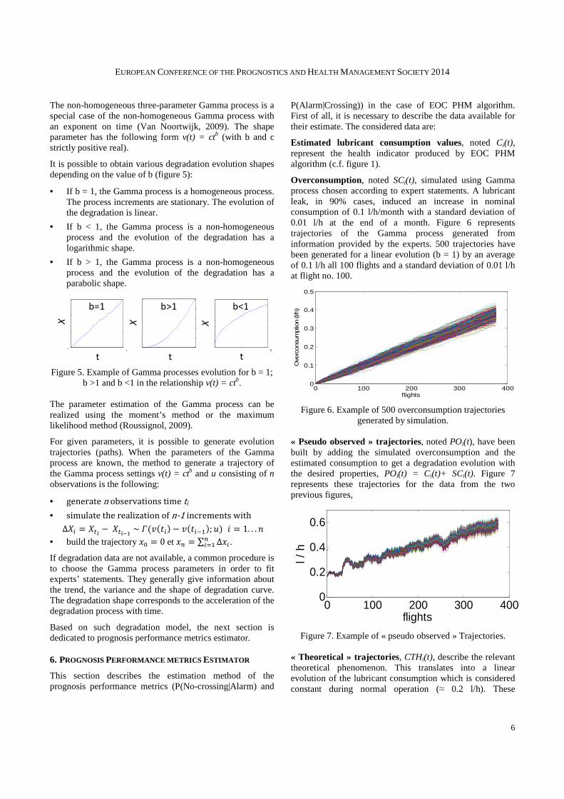
It is possible to obtain various degradation evolution shapes depending on the value of b (figure 5):
• If b = 1, the Gamma process is a homogeneous process. The process increments are stationary. The evolution of the degradation is linear.
• If b < 1, the Gamma process is a non-homogeneous process and the evolution of the degradation has a logarithmic shape.
• If b > 1, the Gamma process is a non-homogeneous process and the evolution of the degradation has a parabolic shape.
Figure 5. Example of Gamma processes evolution for b = 1; b >1 and b <1 in the relationship v(t) = ctb.
The parameter estimation of the Gamma process can be realized using the moment’s method or the maximum likelihood method (Roussignol, 2009).
For given parameters, it is possible to generate evolution trajectories (paths). When the parameters of the Gamma process are known, the method to generate a trajectory of the Gamma process settings v(t) = ctb and u consisting of n observations is the following:
• generate n observations time ti • simulate the realization of n-1 increments with
If degradation data are not available, a common procedure is to choose the Gamma process parameters in order to fit experts’ statements. They generally give information about the trend, the variance and the shape of degradation curve. The degradation shape corresponds to the acceleration of the degradation process with time.
Based on such degradation model, the next section is dedicated to prognosis performance metrics estimator.
6. PROGNOSIS PERFORMANCE METRICS ESTIMATOR
This section describes the estimation method of the prognosis performance metrics (P(No-crossing|Alarm) and
P(Alarm|Crossing)) in the case of EOC PHM algorithm. First of all, it is necessary to describe the data available for their estimate. The considered data are:
Estimated lubricant consumption values, noted Ci(t), represent the health indicator produced by EOC PHM algorithm (c.f. figure 1).
Overconsumption, noted SCi(t), simulated using Gamma process chosen according to expert statements. A lubricant leak, in 90% cases, induced an increase in nominal consumption of 0.1 l/h/month with a standard deviation of 0.01 l/h at the end of a month. Figure 6 represents trajectories of the Gamma process generated from information provided by the experts. 500 trajectories have been generated for a linear evolution (b = 1) by an average of 0.1 l/h all 100 flights and a standard deviation of 0.01 l/h at flight no. 100.
Figure 6. Example of 500 overconsumption trajectories generated by simulation.
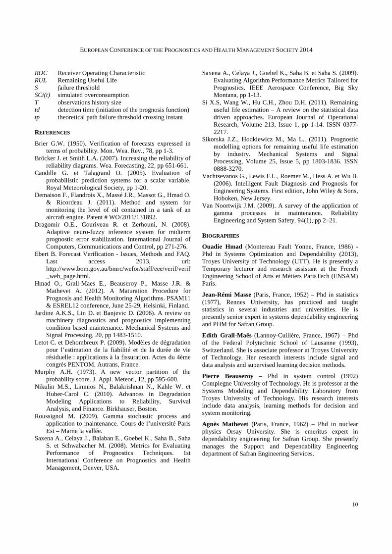
« Pseudo observed » trajectories, noted POi(t), have been built by adding the simulated overconsumption and the estimated consumption to get a degradation evolution with the desired properties, POi(t) = Ci(t)+ SCi(t). Figure 7 represents these trajectories for the data from the two previous figures,
Figure 7. Example of « pseudo observed » Trajectories.
« Theoretical » trajectories, CTHi(t), describe the relevant theoretical phenomenon. This translates into a linear evolution of the lubricant consumption which is considered constant during normal operation (≈ 0.2 l/h). These
0 50 1000
5
10
15
t
x
0 50 1000
2
4
6
8
10
t
x
0 50 1000
1
2
3
4
5
6
7
t
x
b=1 b>1 b<1
X
t t t
X X
0 100 200 300 4000
0.1
0.2
0.3
0.4
0.5
flights
Ove
rcons
um
ptio
n (l/
h)
0 100 200 300 4000
0.2
0.4
0.6
flights
l / h
EUROPEAN CONFERENCE OF THE PROGNOSTICS AND HEALTH MANAGEMENT SOCIETY 2014
7
trajectories correspond to the simulated overconsumption added to the average consumption (CM), CTHi(t)= CM + SCi(t). An example is given in figure 8.
Figure 8. Example of « theoretical » trajectories.
Using these data, the estimation of each prognosis performance metric procedure is described in the two following paragraphs.
6.1. P(NO CROSSING|ALARM)
The estimate of P(No-crossing|Alarm) is, from multiple paths, to determine the proportion of alarms triggered by the prognosis function while the real degradation indicator stays below the failure threshold in the considered time horizon (H). To do this, the procedure is:
For each “pseudo observed” trajectory:
• determine the instant (td) that initiate the prognosis function,
• apply the prognosis function to observations that belong in the interval [td - T, td],
• estimate the probability that observations cross the failure threshold after time horizon H (at td + H),
• if the estimated crossing probability exceeds a limit set at 0.8, an alarm is triggered,
• in case of alarm, identify the “ theoretical” path corresponding to the considered “pseudo observed” trajectory,
• check if the “ theoretical” trajectory has crossed the failure threshold at instant td + H. Increment not justified crossing counter if this is not the case.
This procedure has been applied from the detection time td on each simulated trajectory. Once all trajectories are considered, the ratio of unjustified crossings that represents an empirical estimate of P(No-crossing|Alarm) has been determined. This allowed observing the evolution of this indicator over flights.
6.2. P(ALARM|CROSSING)
This indicator corresponds to the probability of good failure prognosis.
The estimation procedure is:
For each “theoretical” trajectory:
• determine the instant (tp) which corresponds to the instant when the considered “ theoretical” trajectory CTHi(t)cross the failure threshold.
• apply the prognosis function to observations of the corresponding “ pseudo observed” path within the time interval [tp-H-T, tp - H] to estimate the probability that the trajectory crosses the failure threshold at time tp.
• if the estimated crossing probability exceeds a limit of probability set at 0.8, an alarm is triggered and the justified crossing counter is increment.
For each trajectory, this procedure has been applied from the time tp to the end of the observation time. This was repeated for all trajectories. Once all trajectories have been considered, the ratio of justified crossings that represents an empirical estimate of P(Alarm|Crossing) has been determined.
7. CASE STUDY : LUBRICANT OVER-CONSUMPTION
PROGNOSIS
The methodology to evaluate the performance of the prognosis function has been applied to the EOC PHM algorithm. Results are presented on figure 9 and figure 10 for one engine on two different aircrafts.
Each figure is composed of three subfigures:
1. the first one represents the “pseudo observed” trajectories for one engine, the failure threshold (horizontal solid line), the detection threshold (horizontal dashed line) from which the prognosis is initiated, a threshold that indicates that 10% of “ theoretical” paths have crossed the failure threshold (vertical dashed line on the left) and a second threshold indicating that 90% of “ theoretical” paths have crossed the failure threshold (vertical dotted line on the right).
2. the second one represents the ratio of unjustified failure prognosis, P(No-crossing|Alarm), over flights and the 10% and 90% thresholds.
3. the third subfigure represents the ratio of justified failure prognosis, P(Alarm|Crossing), over flights and the 10% and 90% thresholds.
The unjustified crossings ratios are not null. They range from 6% (figure 10), which is acceptable, up to more than 40% (figure 9), which is not acceptable.
These unacceptable values are explained by the noisy nature of estimated consumption. Depending on the learning slope zone of the “pseudo observed” trajectories, the latter may be more or less pronounced which has a direct impact on the
0 100 200 300 4000
0.2
0.4
0.6
flights
l / h
EUROPEAN CONFERENCE OF THE PROGNOSTICS AND HEALTH MANAGEMENT SOCIETY 2014
8
crossing probability. It happens that the slope of a trajectory is important and induces a crossing probability greater than 80%. However, as the estimated consumption falls sharply, the trajectory in question does not cross the failure threshold and therefore gives rise to an unjustified failure prognosis (unjustified removal).
Concerning the justified crossings proportions, they increase over flights to 100% once all paths are above the failure threshold. The noisy nature of the estimated consumptions has also a significant impact there. This is due to the fact that certain trajectories go below the failure threshold for a short time before crossing it again.
However, these non-acceptable performances in terms of P (No-Crossing|Alarm), deserve to be nuanced. It is less damaging to observe an unjustified alarm when the “theoretical” crossing probability is close to 90% than when it is approximately 10%. If the peak of the P(No-crossing|Alarm) curve is close to the flight at 90% threshold this is less damaging than if the peak is nearby the flight at 10% threshold. In terms of justified crossings ratios, P(Alarm|Crossing), deserve to be refined. It is less damaging than P(Alarm|Crossing) is low when the theoretical crossing probability is approximately 10% than when the theoretical crossing probability is approximately 90%. If a large value of the P(Alarm|Crossing) curve appear between flights at 10% and 90% this is less damaging than if this value does not appear until after the flight to 90%.
The accuracy of estimated consumption has a direct impact on the performance of the prognosis function. It is therefore necessary to improve the accuracy of estimated consumption in order to re-evaluate the performance. This is discussed in the next section.
Several proposals have been made to improve the performance of the prognosis function:
• First, as mentioned above, stabilization of the precision estimated consumption. It appears clearly that the fluctuation of the paths causes unjustified failure forecasts or fail to forecast failure,
• If this is not sufficient, the limit of probability, arbitrarily set to 0.8, which gives rise to an alarm and removal can be modified. Increasing this limit of probability is likely to diminish the number of unjustified crossing predictions,
• The tuning of the history window size (T) or the prognosis horizon size (H).
However, the impact of the two last proposals cannot be assessed until the accuracy of the estimated consumptions is not improved.
In this perspective, corrections of consumption have been realized taken into account some missing fills. These improvements are to acting on the extraction of lubricant levels to improve the final estimate of consumption. Inaccuracies remain however. They are explained by the omission of one or more fillings when some flights are missing.
These consumption estimates were used to estimate the performance of the prognosis function again. The estimation procedure remains unchanged. The results in figure 11Figure and figure 12 are presented in a similar way and on the same data as figure 9 and figure 10.
For engine 1 of aircraft 4 (figure 11), the results after changes appear poorer than before. This is again due to the estimated consumptions. It would appear that other fillings than those already corrected have been omitted. This explains the increases in consumption followed by decreases
Conclusions are the same for engine 1 of aircraft 5 (figure 12) with not justified crossing ratio of 98% just before crossing the failure threshold. This is due to the fact that, due to noise, the trajectories are decreasing just before crossing the failure threshold. It follows that the majority of crossing probabilities estimated on the history window (T) prior to this phenomenon are greater than 80% resulting in a high proportion of unjustified crossings. It appears that results strongly depend of each engine and it is not easy to have a general conclusion.
In the aeronautical field, the formalization of PHM systems and their performance requirements are defined from an operational point of view. This often results that used performance indicators are different from those derived
from the literature. The performance evaluation is to adapt indicators from the literature to industrial needs or to define new ones. The adaptation of these indicators is to ensure their relevance with regard to the expected performance requirements.
The performance of PHM systems requirements defined by operators are the ratio of unjustified failure prognosis, P(No-crossing|Alarm), and the ratio of justified failure prognosis, P(Alarm|Crossing). The estimation of each of these probabilities procedure was undertaken by the prognosis process of lubricant overconsumption. The required data for their estimate are: the estimated consumptions, simulated overconsumption using Gamma process, “pseudo observed” trajectories and “theoretical” trajectories. This has allowed establishing a method to perform empirical estimation of the performance of the prognosis function.
The estimation of performance indicators and the analysis of the results have been illustrated by the maturation of the prognosis function in the case of EOC PHM algorithm.
Results show that:
• the accuracy of estimated consumptions have a direct and significant impact on the performance of the prognosis function,
• prognosis is very sensitive to the noise of the signal which it uses to make the prognosis.
Extraction of lubricant levels improved partially stabilized consumption estimate. This is not sufficient for the use of the prognosis function. We should continue in this direction in order to correct missing fills. Once these done, other optimizations may be considered:
• the limit of probability, arbitrarily set to 0.8, which gives rise to an alarm and a removal could be optimize,
• the size of the history window, T, and/or the prognosis horizon, H, could be tune in order to improve results .
Another possible improvement would be to change the prognosis method. This perspective is being studied. A second prognosis function using particle filtering has been developed. After maturation of the latter, the performance of the two prognosis methods (linear regression and particle filtering) will be compared.
NOMENCLATURE
BS Brier Score Ci(t) estimated lubrication consumption values CM average consumption CTHi(t) theoretical trajectories EOC engine Oil Consumption H prognosis horizon size P(Alarm| Crossing) ratio of justified removals P(No Crossing| Alarm) ratio of not justified removals PHM Prognostics and Health Management POi(t) Pseudo Observed trajectories
EUROPEAN CONFERENCE OF THE PROGNOSTICS AND HEALTH MANAGEMENT SOCIETY 2014
10
ROC Receiver Operating Characteristic RUL Remaining Useful Life S failure threshold SCi(t) simulated overconsumption T observations history size td detection time (initiation of the prognosis function) tp theoretical path failure threshold crossing instant
REFERENCES
Brier G.W. (1950). Verification of forecasts expressed in terms of probability. Mon. Wea. Rev., 78, pp 1-3.
Bröcker J. et Smith L.A. (2007). Increasing the reliability of reliability diagrams. Wea. Forecasting, 22, pp 651-661.
Candille G. et Talagrand O. (2005). Evaluation of probabilistic prediction systems for a scalar variable. Royal Meteorological Society, pp 1-20.
Demaison F., Flandrois X., Massé J.R., Massot G., Hmad O. & Ricordeau J. (2011). Method and system for monitoring the level of oil contained in a tank of an aircraft engine. Patent # WO/2011/131892.
Dragomir O.E., Gouriveau R. et Zerhouni, N. (2008). Adaptive neuro-fuzzy inference system for midterm prognostic error stabilization. International Journal of Computers, Communications and Control, pp 271-276.
Ebert B. Forecast Verification - Issues, Methods and FAQ. Last access 2013, url: http://www.bom.gov.au/bmrc/wefor/staff/eee/verif/verif_web_page.html.
Hmad O., Grall-Maes E., Beauseroy P., Masse J.R. & Mathevet A. (2012). A Maturation Procedure for Prognosis and Health Monitoring Algorithms. PSAM11 & ESREL12 conference, June 25-29, Helsinki, Finland.
Jardine A.K.S., Lin D. et Banjevic D. (2006). A review on machinery diagnostics and prognostics implementing condition based maintenance. Mechanical Systems and Signal Processing, 20, pp 1483-1510.
Letot C. et Dehombreux P. (2009). Modèles de dégradation pour l’estimation de la fiabilité et de la durée de vie résiduelle : applications à la fissuration. Actes du 4ème congrès PENTOM, Autrans, France.
Murphy A.H. (1973). A new vector partition of the probability score. J. Appl. Meteor., 12, pp 595-600.
Nikulin M.S., Limnios N., Balakrishnan N., Kahle W. et Huber-Carol C. (2010). Advances in Degradation Modeling Applications to Reliability, Survival Analysis, and Finance. Birkhauser, Boston.
Roussignol M. (2009). Gamma stochastic process and application to maintenance. Cours de l’université Paris Est – Marne la vallée.
Saxena A., Celaya J., Balaban E., Goebel K., Saha B., Saha S. et Schwabacher M. (2008). Metrics for Evaluating Performance of Prognostics Techniques. 1st International Conference on Prognostics and Health Management, Denver, USA.
Saxena A., Celaya J., Goebel K., Saha B. et Saha S. (2009). Evaluating Algorithm Performance Metrics Tailored for Prognostics. IEEE Aerospace Conference, Big Sky Montana, pp 1-13.
Si X.S, Wang W., Hu C.H., Zhou D.H. (2011). Remaining useful life estimation – A review on the statistical data driven approaches. European Journal of Operational Research, Volume 213, Issue 1, pp 1-14. ISSN 0377-2217.
Sikorska J.Z., Hodkiewicz M., Ma L.. (2011). Prognostic modelling options for remaining useful life estimation by industry. Mechanical Systems and Signal Processing, Volume 25, Issue 5, pp 1803-1836. ISSN 0888-3270.
Vachtsevanos G., Lewis F.L., Roemer M., Hess A. et Wu B. (2006). Intelligent Fault Diagnosis and Prognosis for Engineering Systems. First edition, John Wiley & Sons, Hoboken, New Jersey.
Van Noortwijk J.M. (2009). A survey of the application of gamma processes in maintenance. Reliability Engineering and System Safety, 94(1), pp 2–21.
BIOGRAPHIES
Ouadie Hmad (Montereau Fault Yonne, France, 1986) - Phd in Systems Optimization and Dependability (2013), Troyes University of Technology (UTT). He is presently a Temporary lecturer and research assistant at the French Engineering School of Arts et Métiers ParisTech (ENSAM) Paris.
Jean-Rémi Masse (Paris, France, 1952) – Phd in statistics (1977), Rennes University, has practiced and taught statistics in several industries and universities. He is presently senior expert in systems dependability engineering and PHM for Safran Group.
Edith Grall-Maës (Lannoy-Cuillère, France, 1967) – Phd of the Federal Polytechnic School of Lausanne (1993), Switzerland. She is associate professor at Troyes University of Technology. Her research interests include signal and data analysis and supervised learning decision methods.
Pierre Beauseroy – Phd in system control (1992) Compiegne University of Technology. He is professor at the Systems Modeling and Dependability Laboratory from Troyes University of Technology. His research interests include data analysis, learning methods for decision and system monitoring.
Agnès Mathevet (Paris, France, 1962) – Phd in nuclear physics Orsay University. She is emeritus expert in dependability engineering for Safran Group. She presently manages the Support and Dependability Engineering department of Safran Engineering Services.