Operations Research A Statistical Technique for Comparing Heuristics

RESEARCH CONlRh9UTIONS

Management Science, Operations Research

A Statistical Technique Harvey J Greenberg Edit or for Comparing Heuristics:

An Example from Capacity Assignment Strategies in Computer Network Design RICHARD E. NANCE, ROBERT L. MOOSE, JR., and ROBERT V. FOUTZ

ABSTRACT: An analysis of variance (ANOVA) model is developed for determining the existence of significant differences among strategies employing heuristics. Use of

the model is illustrated in an application involving capacity assignment for networks utilizing the dynamic hierarchy architecture, in which the apex node is reassigned in response to changing environments. The importance of the model lies in the structure provided to the evaluation of heuristics, a major need in the assessment of benefits of artificial-intelligence applications. A nested three-factor design with fixed and random effects provides a numerical example of the model.

1. INTRODUCTION The need to apply objective discrimination to the performance of algorithms is evident throughout the mathematical sciences, but most prevalently in the domain of heuristic techniques or heuristic programming. Lacking the definitive qualifications imparted by analytical methods, the heuristic techniques must be judged on a “results” basis in an experimental setting. Such a judgment is often complicated by

(1) a large number of heuristics from which only a small set of alternatives can be examined;

(2) no convenient or convincing basis for selecting alternatives;

(3) no clear ordering among alternatives based on the results obtained;

The research effort of Nance and Moose was supported in part by the Naval Sea Systems Command under Contract N60921-83GA165 through the Systems Reseach Center at Virginia Tech.

0 1987 ACM 0001.0782/87/0500-0430 750

(4) the appearance of interaction among fa.ctors in the experimental setting, complicating the discrimination of performance differences.

Lin and Kernighan describe the means for evalu- ating heuristic approaches by applying statistical analyses to solution techniques in traveling- salesman problems [lo] and to graph partitioning problems [5]. In a subsequent paper, Lin [9, p. 401 notes the difficulty of objectively comparing heuristic algorithms for solving combinatorial optimization problems. Operation counts or examination of the structure of algorithms, although employed in the past for evaluation, do not suffice for definitive discrimination. Even experimental comparison must be applied knowledgeably to permit valid evaluation conclusions.

The subject of this paper is the presentation of an analysis of variance (ANOVA) model that h,as general applicability to the statistical evaluation of heuristic procedures, and the illustration of the model through application to a computer network design problem. A brief explanation of the network design application is given in Section 2, followed by the heuristic techniques in Section 3. The development of the ANOVA model is explained in Section 4 and illustrated in Section 5. Summary and conclusions constitute the final section.

2. BACKGROUND AND MOTIVATIONS The statistical model and analysis addressed in this paper are motivated by the authors’ research of a topic in the area of local-area network (LAN) design, namely, the link capacity assignment problem for

430 Communications of the ACM May 1987 Volume 30 Number 5

Research Contributions

dynamic hierarchical networks. Detailed discussions of dynamic hierarchical networks (or dynamic hier- archies), a network performance measure, and various capacity assignment strategies are given elsewhere [IS, 141. This information is presented here in condensed form to provide a framework for development of the statistical test procedure and also to serve as an example of its application.

2.1 Dynamic Hierarchical Networks The dynamic hierarchy is an architectural concept for a LAN that is embedded within an application system displaying the following characteristics:

(1)

(2)

(3)

Real-time or time-critical response is manda- tory;

demands in the application system can vary and alter the load placed on individual elements of the embedded LAN (the message traffic and the processing requirements);

the encapsulating system has stringent requirements for high capability, reliability, adaptabil- ity, and survivability that must be imparted as requirements of the LAN.

The dynamic hierarchy represents a generaliza- tion of the conventional tree-structured architecture in which the network operates under a centralized, strictly hierarchical mode of control. An overriding characteristic of these conventional (static) hier- archies is that at the root of a tree-structured topology exists a single (apex) node that has primary control responsibility. Secondary capabilities filter down through the remainder of the network in a hierarchical manner. A dynamic hierarchical network is a hierarchical network in which the node assuming the apex position can vary among a designated subset of nodes.

A dynamic hierarchy is suitable for an application demanding quite different services under varying external situations. For each situation an apex node (and a corresponding hierarchical topology) is designated as the one most beneficial for the particular situation. At any given instant, the network con- forms to one of the specified topologies. When a situation change occurs, the network undergoes a transi- tion, with the designated node becoming the apex of the hierarchy corresponding to the reconfigured topology. In the architectures considered to date, the network topology remains static: Once the network is constructed, the interconnections remain fixed. However, the network topology is logically variable as a result of changes in the apex node (and the corresponding changes in the hierarchical distribu- tion of contro1 responsibilities).

2.2 Performance and Capacity Assignment Mean network delay is taken as the primary measure of performance of the dynamic hierarchy. For conventional networks, given the assumptions made by Kleinrock [6, 71, a closed form expression for mean delay is derived through the application of elementary queueing theory. This expression is extended as follows to provide an approximate measure of delay in the dynamic hierarchy:

Define

lti) = long-run probability of occurrence of configuration (and environment) i.’

Considering each configuration i separately (as if it were a static hierarchy), let TcO denote mean network delay, as derived by Kleinrock, for that configuration. We then take the measure of network delay for the dynamic hierarchy to be the weighted sum of the individual configuration mean delay values. That is,

where M is the number of possible configurations, Although this is only an approximation of mean delay, it is still useful for the purpose of comparing capacity assignment strategies within the class of dynamic hierarchical networks.

Now let

L = number of links, Cj = capacity of link j, C = total network capacity,’ and

T max = upper bound on mean network delay.

The dynamic hierarchy capacity assignment problem can be formulated as follows:

Given (I) the set of network configurations, and (2) for each configuration (environment) i, its (a) stationary probability of occurrence ,$(‘I and (b) traffic characterization, minimize

Cc $ Cj, j=l

with respect to

subject to

{Cj:j = 1, 2, . . . , L],

Two distinct methods are used to create approxi-

‘We assume that the underlying model of the environment is such that these probabilities are nonzero.

‘All of the strategies assume a unit cost function. Thus total capacity is equal to total cost.

May 1987 Volume 30 Number 5 Communications of the ACM 431


mate solutions to this problem. The first method yields a set that we refer to as the probabilistic strategies. Each of these strategies is defined in a way similar to the construction of the dynamic hierarchy delay measure. Considering each configuration i separately, for each link j, let Cl” denote an allocation of capacity for link j that is in some sense optimal for the static network represented by configuration i. Then, for the capacity of link j, set

where kj represents a minimum required capacity term and C’y’ is related to C’ji’ (the exact form of C’g) depends on whether kj = 0 or not). Among this set of probabilistic strategies, the two most promising are labeled DSR and DMX.

The second method, algorithmic in nature, produces a set that we refer to as the heuristic strategies. First, a collection of capacity assignment heuristics are defined. These heuristics and the func- tions they perform are

generation of an initial set of assignments:

SETLOW, SETHIGH;

choice of a link for a capacity increase:

ADDl, ADD2;

choice of a link for a capacity decrease:

DROPl, DROP2;

increase or decrease of all capacities:

ADDALL, DROPALL.

Various combinations of these heuristics are then formed to produce a set of composite assignment strategies. (This approach is employed extensively by Maruyama et al. to construct design algorithms for conventional networks; e.g., see [Ill.) The strategies in this set are referred to as HEURISTICl, HEURISTIC2, . . . , HEURISTIC12.

3. DETERMINATION OF BEST STRATEGIES THROUGH ANOVA PROCEDURES Having developed the sets of probabilistic and heuristic strategies, comparison of these strategies for the purpose of identifying the best within each set and the best overall becomes a necessary task. This task is performed by analyzing the results of various collections of capacity assignment experiments.

For each set of strategies, the experimentation consists of the generation of capacity assignments under nine different sets of parameters for each of six test networks. For each network three sets of stationary configuration probabilities are used. Under each set assignments are generated for three

different delay constraints. Note that, for a given network, the topologies and set of link traffic rates remain fixed throughout the experimentation. Differ- ent experiments are defined by varying the stationary configuration probabilities and maximum mean delay through nine combinations of values. (Hence- forth, a selection of values for maximum mean delay and stationary configuration probabilities is referred to as an auxiliary parameter setting or a-setting.) A single experiment consists of applying the members of a set of strategies to a particular network/a-setting combination. The output is a set of assignments and the resulting value of total cost (capacity) that constitute the basis for the evaluation.

In the absence of a theoretical (analytic) basis for comparing the strategies, alternate method:s are employed. The methods used here are derived from statistical hypothesis testing and parameter estima- tion procedures. Specifically, ANOVA techniques are used to determine whether differences exist in the effects of the assignment strategies. That is, it is determined whether at least one strategy produces assignments that are different from (better than) those produced by the remaining strategies. The ANOVA computations produce as byproducts point estimates of certain population means, which provide additional information on the effects of the strategies.

One normally applies statistical techniques to observed random variables. Clearly, neither the in- put to nor results from our experiments constitute conventional random variables. However, the ration- ale behind the approach is as follows:

Consider the six test networks as representative of the members of a conceptually infinite population of (dynamic hierarchical) test networks. Also, consider the nine a-settings used with each network as representative of a conceptually infinite population of a-settings. Then the total cost values associated with each strategy are viewed as random variables-their values vary according to a random selection of different network and a-setting combinations :from the respective populations.

ANOVA is applied to the observed cost values as if the six test networks and their a-settings are randomly sampled from their underlying populations. As a consequence, when one concludes from this analysis that the strategies differ in their effects on total cost, the results extend beyond the network/ a-setting combinations used in the study to include strategy differences over all possible network/ a-setting combinations through sampling the underlying network and a-setting populations. The network and a-settings need not be randomly sampled



in practice. However, essential in interpreting these general conclusions is the delineation of the bound- aries of the conceptual populations from which the networks and the corresponding a-settings in the study can be reasonably regarded as a random sample (cf. Sheffe [15, p. ZX]).

In a conventional ANOVA, one is concerned with the identification of variability due to random observation (error) effects. When one concludes that the treatment effects are different, one is concluding that different treatments and not random error effects contribute significantly to variability in the results. As noted below, the statistical model dis- cussed here does not include random error effects (from data or otherwise). The randomness in our data is induced by the choice of networks and a-settings.

The experimental design is a variant of a three- factor, nested design with fixed and random effects. To derive the appropriate model, assume that the factors

(1) (choice of) network, (2) assignment strategy, and (3) (choice of) auxiliary parameter setting

all contribute to differences in total cost values. Under the stated sampling assumption, network and a-setting are random effects. A-setting is a nested factor within networks. The assignment strategy is a fixed effects factor.

In addition to the effects of factors (l), (2), and (3), the following effects must also be included:

(4) network/strategy interaction, and (5) a-setting/strategy interaction.

Network/a-setting interaction and second-order interaction effects are absent since a-setting is nested within rather than crossed with network.

The combination of effects from sources (l)-(5) produces the following model:

Xijk = /L + Ni + P(t)j + Sk + (NS)ik + (PS)(i)jk

where

xijk = total cost value resulting from the application of strategy k to network i and its jth a-setting;

p = mean of parent population; Ni = main effect of network i, i = 2, 3, . . . , 6;

Pci)j = main effect of a-setting j within network i, j = 1, 2, . . . , 9;

Sk = main effect of strategy k, k = 1, 2, . . . , T; T = number of strategies;

$S)ik = interaction effect of network i and strategy k;

(PS)ti,,k = interaction effect of a-setting (i) j and strategy k.

Two aspects of this model require elaboration. First, the equalities

Sk = C(k - /6 k = 1, 2, . . . , T,

where pk is the mean of the treatment population corresponding to strategy k, define the main strategy effects. Since strategy is a fixed effects factor, the T strategies are viewed as an exhaustive sample of the population of strategies (treatment levels), which implies

T

CL = $ ,F; CLk.

so,

T 7 T

c Sk = kgl &k - d = c k=l

k=l Ilk - TL‘ = 0.

A second important aspect of the model of xijk is its lack of a random error factor. In formulating a model for ANOVA, one normally assumes that each treatment observation is affected by a random error component. Applied to this model, such an assumption would add an error term tijk to each xijk. The deterministic nature of assignment strategies distin- guishes this problem from those that lead to conventional ANOVA models. A given network/a-setting/ strategy combination determines capacities and unique total-cost values. Replication of the assignment process with the same combination algorithmi- cally produces identical (error-free) values. Hence the model correctly reflects the absence of random error effects in the xijk.

In general, ANOVA with this statistical model requires the following assumption:

(1) (NiJ, {Po)jJ, {(NS)ik), and ((PS)(i)jk] are random samples from independent normal populations with mean zero and variances &, a$, a&s), and [r&s), respectively.

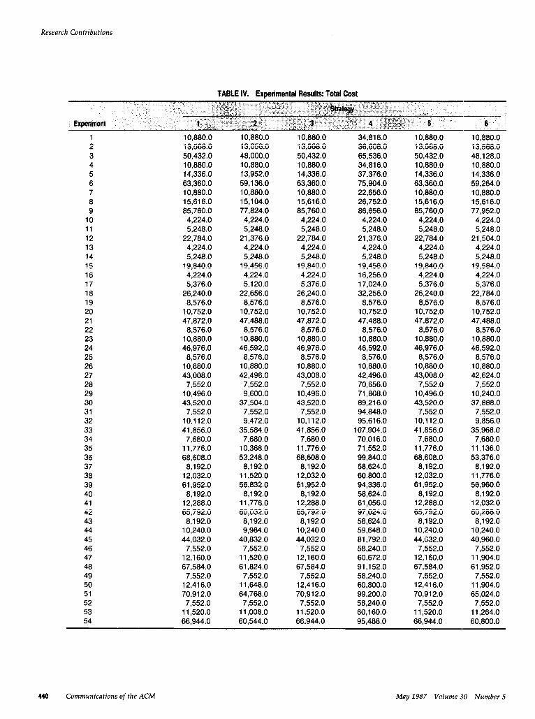
The classical hypothesis testing procedures for ANOVA models are known to be valid under this assumption. However, (1) is too restrictive for our purpose since it implies that the xijk are independent and normally distributed and, consequently, that no two observations (total costs) may have the same value. The data in Table IV in the Appendix show that observations do take the same value, and so assumption (1) must be relaxed.

Jensen and Good [3] have shown that all statistical inference procedures that are valid under (1) remain valid if the following assumption holds in its place:



Source of variance

Networks A-settings Strategies Network/strategy interaction A-setting/strategy interaction Total

TABLE I. Analysis of Variance (total cost)

Degrees of freedom Mean square

101.3543 5 20.2709 319.4691 48 6.6556

99.1074 11 9.0098 46.5195 55 0.8458 37.1555 528 0.0704

603.6059 647 0.9329

(1) INi], IP[i)jIt i(NShl, and i(PS)(i)jkI are random samples from populations that are jointly symmetrically distributed about zero with variances ak, crZ, g&s), and a&s), respectively.

A population is said to be normally distributed with an atom at the point p if the variable of interest equals p with positive probability and is normally distributed with mean p otherwise. The data in the Appendix could arise from our model for Xijk if the random effects Ni, P(i),, and (NS),k are from normal populations with atoms at zero and if, for each i, j,

tps hi),k is from a normal population with an atom at -Sk. Under this assumption the common value X+ = X#‘, for fixed a-setting j within network i, would RSLllt if (Ps)(i]jk = -Sk, (PS)(r)$’ = -Sk’, and (NS);k = (NS)ik, = 0 in our model. The common value xijk = xi’j’k for fixed heuristic k would result if Ni = Ni, = Pci)j = Pci,)j, = (NS)ik = (NS),*k = 0 and (pS)[iJ,k = (ps)[iT)j’k = -Sk. Finally, llOk that, ifHo:SI=Sz= . . . = ST = 0 is true and there is no difference in the main effects of the strategies, then all of the random effects are jointly symmetrically distributed with atoms at zero, (1’) holds, and the standard test for Ho remains valid.

Lin and Rardin [8] propose a related ANOVA model for comparing algorithms that solve integer linear programming problems. This model differs from the above by combining all random effects into a single “random problem” effect. In contrast, we prefer to represent the random effects of networks and a-settings separately in our model, providing the added flexibility to examine separately the main effects of networks and a-settings and their inter- actions with strategies.

4. A NUMERICAL EXAMPLE This section, together with the data contained in the Appendix, provides a numerical example of the statistical approach. In this example we compare HEURISTICl, HEURISTICS, . . . , HEURISTIC12 on the basis of total cost. The figures and tables in the Appendix, which contain all the information necessary to perform the capacity assignment experiments and the analysis, are subdivided as follows:

(1

(2)

(3)

(4)

Network topologies (Figure 1). Only one configuration is illustrated for each network. These illustrations show the physical interconnections for the networks. Note that networks 4-6 have identical topologies, but differ in their traffic statistics and a-settings. Network statistics (Figure 2). These (traffic) statistics consist of throughput, mean message length, and individual link arrival rates. Experiment control data (Figure 3). A-settings are formed by taking various combinations of these data. Experimental results (Table IV). These total-cost values form the basis for the statistical analysis of the example. (As noted below, the analysis actually uses the natural logarithm of these values.)

For the comparison of this example, we have

xijk = (log of) total cost 3 of network i with a-setting i under strategy k (HEURISTICk),

Sk = (main) effect of strategy k on total cost, and a&s) = variance of network/strategy interaction

effects on total cost.

The test for strategy effects is

Ho:SI=S*= ... =&=O

against the alternative

H,: Sk # 0 for at least one k;

the test statistic is

MSs Fs=----= S&/l 1

M~(Ns, SSlNS)/55

the critical value at level a! is F,~,ll,SS. The test for network/strategy interaction is

&:C&!Ns) = 0

against

H,: a$,s) > 0.

‘In an attempt to achieve homogeneity of variance. the transform log.(x) is applied to the data before performing the ANOVA calculations.


This test has test statistic

MS(NS] _ ss(~s)/55 FINS) = ~ -

MS(PS, SS(ps)/528

(where the “(PS)” subscripts denote a-setting/ strategy interaction statistics) and critical value F di5.528~

The ANOVA computations are summarized in Table I. For the first test, these values yield a test statistic Fs = 10.6524. At a significance level of (Y = 0.05, the critical value is Fo.05,11,55 = 1.9725. We reject Ho and conclude that the strategies are different in their effects on total cost. Similarly, we reject the null hypothesis in the second test. The applica- ble statistic values are FINS) = 12.0142 and Fo.05,55,528 < Fo.05,55,200 = 1.40. Thus we must partially attribute the variability of total cost to interaction between networks and strategies.

Having concluded that differences in strategy effects exist, we proceed with multiple comparisons to characterize these differences more precisely. Our multiple comparisons procedure follows the two- stage approach proposed by Fisher [2] (cf. Miller [12, p. 901). Stage one is the F test for H,:S, = SZ = . . . = S12 = 0, at significance level (Y = 0.05, that is summarized in Table I. Had this F test not rejected Ho, the analysis would have found no significant differences among the main strategy effects without proceeding to step two. When the F test is significant, pairwise comparisons among the effects S1, SZ, . . . , ST2 may then be made with appropriate a-level tests at stage two. If the test comparing S; and Sj is significant, then Si and Sj are considered to be different in the final conclusion. Since the stage one F test is performed at level (Y, the experimentwise error rate is also LY for the joint conclusion from the simultaneous


TABLE II. Mean Performance Levels (total cost)

Strategy Mean level

HEURISTIC1 9.6552 HEURISTIC2 9.6130 HEURISTIC3 9.6552 HEURISTIC4 10.5429 HEURISTIC5 9.6552 HEURISTIC6 9.6230 HEURISTIC7 9.6282 HEURISTIC8 9.6130 HEURISTIC9 9.6552 HEURISTIC1 0 10.5396 HEURISTIC1 1 9.6401 HEURISTIC1 2 10.5377

tests of stage two. Finally, note that since all pairwise comparisons (among S,, SZ, . . , Sll) may be investigated during stage two, it is appropriate to perform only a subset of these that may be suggested by the data. The experimentwise error rate then remains no larger than CL

Table II suggests that the strategies may fall into two groups because strategies 4, 10, and 12 perform about equally poorly and the remaining strategies perform about equally well. Accordingly, we replace all pairwise comparisons of stage two by F tests for the equality of effects within the following groups of heuristics:

(A) G, = (HEURlSTlCk, k = 1, 2, 3, 5, 6, 7, 8, 9, 11) (B) (HEURISTlCk, k = 1, 2, 3, 5, 6, 7, 8, 9, 11, 12) (C) (HEURlSTlCk, k = 1, 2, 3, 5, 6, 7, 8, 9, 10, 11) (D) {HEURlSTlCk, k = 1, 2, 3, 4, 5, 6, 7, 8, 9, 11) (E) G, = {HEURlSTlCk, k = 4, 10, 121

Table III contains the test statistics, critical values,

TABLE III. Results of Multiple Comparisons

Strategy Network/strategy interaction

Test statistic’ Critical Rejact Test statistic’ ClitiCSI Test and value value HO and value value

A Fs = $$ = 0.0220 ~~~~~~~~~~ = 2.12 No F(M) = 2 = 0.0227 Fo.05.40.52a A 1.4725

B Fs = g = 5.1571 Fo.05.9.55 = 2.06 Yes F(m) = !J!z& = 5.9233 MS&,

Fo.05.45.528 s 1.455

C Fs = MS:

- = 5.2140 MS &,

Fo.o5.s.~s = 2.06 Yes F(m) = L?!zi& = 5.8631 MS $s,

Fo.05.45.528 h 1.455

D Fs = MSQ = 5.2523 MS $a)

Fo.05.9.55 = 2.06 Yes F - !!!%I = 5.9247 C-J’) - MS&, Fo.05.45.528 -?- 1.455

E Fs = $$ = 0.00041 Fo.05,2,5s = 3.17 No F(Ns) = MsFN5) = 0.00057 MS $5,

~0.05.10.523 * 1.89

‘MS’ = mean square statistic from ANOVA table for comparison i. MS’ = mean square statistic from Table I.

Reject HO

No

Yes

Ye5

Yes

No



and results of the stage-two multiple comparisons. Note, for example, that in (A) the test statistics are

MS<

Fs = MS &

MS $VSJ and FtNs) = 0

MS UPSI ’

where, for increased precision, MS&s) and MS&) are chosen from the table of the stage-one ANOVA computations (Table I) rather than from the table for (A). The mean squares MS< and MS&s, are chosen from the table for (A). The corresponding critical values are F0.05.8.55 and FO.O5,40.528.

With experimentwise error rate (Y = 0.05, the joint conclusion from the simultaneous tests in Table III is that no significant difference exists among the heuristics in G1 (test A); no significant difference exists among the heuristics in Gz (test E); and the heuristics in G, and G2 differ from each other (tests B, C, and D). The practical consequence is that the heuristics in G, are to be preferred over those in Gz.

5. CONCLUSIONS In the course of exploring design strategies for the dynamic hierarchy, a new concept in reconfigurable network architectures, the authors have derived a statistical model and applied the resultant test procedure to compare the effects of these strategies.

ANOVA techniques are used to determine whether significant differences exist among assignment strategies. When differences are detected, multiple comparison procedures are used to characterize the differences.

The statistical technique is potentially quite general. Both fixed (strategy) and random (network, a-setting) effects are included in the model. The approach does not preclude the existence of random error effects. Additionally, in cases where our model does not apply directly to the data of interest, this paper illustrates the method by which conventional ANOVA techniques may be applied in a variety of experimental settings.

A referee has noted that the technique of entropy data analysis (see Jones [4]) may offer some inherent advantages over the more traditional ANOVA approach, particularly with regard to the assu:mptions about the underlying populations for the component effects. Time and space preclude development of a comparative treatment in this paper.

Finally, we offer this application of ANOVA to the discrimination among heuristics as yet another example of a problem domain in the intersection of computer science and statistics. This domai-n adds yet another fertile area of investigation to those suggested recently by Barlow and Singpurwalla. [l].

APPENDIX A

(a) Network 1 (c) Network 3

(b) Network 2 (d) Networks 4,5, and 6

FIGURE 1. Network Topologies



(a) Network 1

Number of configurations: 3; Number of links: 13

Configuration Throughput 1 49.4953 2 58.6475 3 8.2955

Mean message length: 100.0

Arrival rates

Configuration Link 1 2 3

(c) Network 3


Configuration Throughput 1 17.7751 2 9.3854 3 7.7540 4 10.0783


Arrival rates

Link Configuration

1 2 3 4

1 3.4190 6.9229 1.7588 2 2.0515 3.6077 9.5031 3 9.2433 4.6049 0.2534 4 3.1729 4.1172 7.7430 5 6.2562 6.9361 7.2866 6 9.0486 6.0137 7.2008 7 1.1967 2.3302 4.7877 8 1.8832 3.4728 6.8186 9 0.1826 6.2331 1.4092

10 7.3828 9.6381 2.3904 11 2.7075 9.3868 4.8310 12 4.5558 4.7949 4.5601 13 8.4576 7.9091 1.8160

(b) Network 2


Configuration Throughput 1 2.7017 2 16.8263


Arrival rates

Link Configuration

1 2

9.1201 2.8299 1.2963 4.8119 2.5600 1.7485 4.9787 8.4113 5.4387 6.1683 7.0878 9.2017 8.3500 1.8290 4.7762 3.8477 9.9332 8.6454 3.5377 7.1967 9.1846 5.1439 7.0931 5.4839 7.5754 3.4996 5.1247 8.6585 1.1359 7.4501 1.5486 5.3842 9.5691 4.2993 5.6052 2.0882

(d) Network 4




Arrival rates

Link Configuration

1 2 3

1 1.0416 6.4589 2 5.4727 5.9396 3 0.0430 7.0999 4 0.7439 7.9838 5 1.1552 5.1225 6 3.7621 3.9253

2 3 4 5 6 7 8 9

10 11 12 13 14

0.6000 0.5000 0.6000 0.8500 0.7500 0.9000 0.8500 0.7500 0.7000 0.6000 0.5000 0.5000 5.0000 1 .oooo 0.8000 1 .oooo 4.5000 1.5000 1 .oooo 1 .oooo 4.5000 8.5000 0.4000 0.3000 9.5000 0.6500 0.6000 0.5000 6.5000 1 .ooOO 0.7500 8.0000 1.5000 0.5000 0.6000 7.0000 0.7500 0.8500 7.5000 3.2000 0.1000 0.1000

FIGURE 2. Network Statistics



(e) Network 5




Arrival rates

Link 1

1 0.8060 2 0.9000

4” 0.7500 1 .oooo 5 6.0000 6 4.5000 7 4.0000 8 8.0000 9 9.0000

10 5.8000 11 5.9000 12 3.5000 13 5.0000 14 3.2000

Configuration 2

1 .lOOO 1 SO00

1 1.5000 .oooo 4.0000 5.5000 4.2000 5.0000 4.5000 7.0000 8.0000 6.5000 6.0000 2.5000

3

0.9000 1.4000 1.2000 1 .oooo 5.0000 4.7000 5.8000 5.0000 6.0000 5.0000 4.5000 7.0000 7.1000 2.9000

(f) Network6




Arrival rates

Link

1 2 3 4 5 6 7 8 9

10 11 12 13 14

Configuration 1 2

0.7000 0.8000 0.8600 1.1300 0.9300 1.1300 0.6800 0.7500 5.9000 2.5000 2.7500 4.5000 2.5000 2.6000 8.5000 2.7000 9.5000 2.5800 3.1500 6.5000 3.3300 8.0000 2.0000 3.5500 2.8800 3.4300 3.2000 1.3000

3

0.7500 1.1500 0.9500 0.7500 2.9000 3.1000 4.5000 2.6500 3.3000 3.0000 3.0000 7.0000 7.5000 1.5000

FIGURE 2. Network Statistics (continued)

438 Communications of the ACM Maiy 1987 Volume 30 Number 5


(a) Run 1

Configuration probability sets

Set 1

1 0.3400 2 0.2000 3 0.1000

Design constraints

Iteration 1 2 Constraint value 10.0 1 .O

(b) Run 2


Set

1 2 3

Design constraints

iteration 1 2 Constraint value 10.0 1 .O

Configuration 2

0.3300 0.3000 0.1000

3 0.1

3

0.3300 0.5000 0.8000

(d) Run 4


Configuration Set 1 2 3

1 0.3400 0.3300 0.3300 2 0.2000 0.5000 0.3000 3 0.1000 0.1000 0.8000

Design constraints

Iteration 1 2 3 Constraint value 10.0 1.0 0.1

Configuration 1 2

0.5000 0.5000 0.2500 0.7500 0.8000 0.2000

3 0.1

(c) Run3



1 0.2500 0.2500 0.2500 2 0.3500 0.2000 0.2000 3 0.7000 0.0500 0.0500

Design constraints

Iteration 1 2 3 Constraint value 10.0 1 .O 0.1

(e) Run 5



1 0.3300 0.3300 0.3400 2 0.5000 0.2000 0.3000 3 0.1000 0.8000 0.1000

Design constraints

Iteration 1 2 3 Constraint value 10.0 1.0 0.1

4

0.2500 0.2500 0.2000

(f) Run6



1 0.3300 0.3400 0.3300 2 0.2000 0.3000 0.5000 3 0.1000 0.8000 0.1000

Design constraints

Iteration 1 2 3 Constraint value 10.0 1 .O 0.1

FIGURE 3. Experiment Control Data



TABLE IV. Experimental Results: Total Cost

2 3 4 5 6 7 8 9

10 11 12 13 14 15 16 17 18 19 20 21 22 23 24 25 26 27 28 29 30 31 32 33 34 35 36 37 38 39 40 41 42 43 44 45 46 47 48 49 50 51 52 53 54

10.880.0 10,880.O 13.568.0 13,056.O 50,432.O 48,000.0 10,880.O 10,880.O 14,336.0 13,952.0 63,360.O 59,136.0 10,880.O 10,880.O 15,616.0 15,104.o 85,760.O 77,824.0

4,224.0 4.224.0 5,248.0 5,248.0

22,784.0 21,376.0 4,224.0 4,224.0 5,248.0 5,248.0

19,840.O 19,456.0 4,224.0 4,224.0 5.376.0 5,120.O

26,240.O 22,656.0 8.576.0 8,576.0

10,752.O 10,752.O 47,872.0 47,488.0

8,576.0 8,576.0 10,880.O 10,880.O 46,976.0 46,592.0

8,576.0 8,576.0 10,880.O 10,880.O 43,008.O 42,496.0

7,552.0 7,552.0 10,496.O 9,600.O 43,520.O 37,504.o

7,552.0 7,552.0 10,112.o 9,472.0 41,856.0 35,584.0

7,680.O 7,680.O 11,776.0 10,368.O 68,608.O 53,248.0

8,192.0 8,192.0 12,032.O 11,520.O 61,952.0 56,832.0

8,192.0 8,192.0 12,288.0 11,776.0 65,792.0 60,032.O

8,192.0 8,192.0 10,240.O 9,984.0 44,032.O 40,832.O

7,552.0 7,552.0 12,160.O 11,520.O 67,584.0 61,824.0

7,552.0 7,552.0 12,416.0 11,648.0 70,912.o 64,768.0

7.552.0 7,552.0 11.520.0 11,008.O 66,944.0 60,544.O

10,880.O 34.816.0 10,880.O 10,880.O 13,568.0 36.608.0 13,568.0 13,568.0 50,432.O 65,536.0 50,432.O 48,128.0 10,880.O 34.816.0 10,880.O 10,880.O 14,336.0 37.376.0 14,336.0 14,336.0 63,360.O 75,904.o 63.360.0 59.264.0 10,880.O 22,656.0 10.880.0 10.880.0 15,616.0 26,752.0 15,616.0 15,616.0 85,760.O 86,656.0 85,760.O 77,952.0

4,224.0 4,224.0 4.224.0 4.224.0 5,248.0 5,248.0 5.248.0 5,248.0

22,784.0 21,376.0 22,784.0 21,504.o 4,224.0 4,224.0 4,224.0 4,224.0 5,248.0 5.248.0 5,248.0 5,248.0

19,840.O 19,456.0 19,840.O 19,584.0 4,224.0 16,256.0 4,224.0 4,224.0 5,376.0 17,024.O 5.376.0 5,376.0

26,240.O 32,256.0 26,240.O 22,784.0 8,576.0 8,576.0 8,576.0 8,576.0

10,752.O 10,752.O 10.752.0 10,752.O 47,872.0 47,488.0 47.872.0 47,488.0

8,576.0 8,576.0 8,576.0 8.576.0 10.880.0 10,880.O 10.880.0 10,880.O 46.976.0 46,592.0 46,976.0 46,592.0

8,576.0 8,576.0 8,576.0 8.576.0 10.880.0 10,880.O 10.880.0 10,880.O 43,008.O 42,496.0 43.008.0 42,624.0

7,552.0 70,656.O 7,552.0 7.552.0 10,496.O 71,808.O 10.496.0 10,240.O 439520.0 89,216.0 43,520.O 37,888.0

7,552.0 94,848.0 7,552.0 7,552.0 10,112.o 95,616.0 10,112.o 9,856.0 41.856.0 107,904.o 41,856.0 35,968.0

7,680.O 70,016.O 7,680.O 7,680.O 11.776.0 71,552.0 11,776.0 11,136.0 68,608.O 99,840.O 68,608.O 53,376.0

8.192.0 58,624.0 8,192.0 8,192.0 12,032.O 60.800.0 12,032.O 11.776.0 61,952.0 94,336.0 61,952.0 56.960.0

8.192.0 58,624.0 8,192.0 8,192.0 12,288.0 61,056.O 12,288.0 12,032.O 65,792.0 97,024.o 65,792.0 60,288.O

8.192.0 58.624.0 8,192.0 8.192.0 10,240.O 59,648.0 10,240.O 10,240.O 44,032.O 81,792.0 44,632.O 40,960.O

7.552.0 58,240.O 7,552.0 7.552.0 12,160.O 60,672.O 12,160.O 11,904.o 67,584.0 91,152.0 67.584.0 61,952.0

7.552.0 58,240.O 7,552.0 7.552.0 12.416.0 60,800.O 12.416.0 11,904.o 70,912.o 99,200.o 70,912.o 65,024.O

7,552.0 58,240.O 7,552.0 7,552.0 11,520.O 60,160.O 11,520.O 11,264.0 66,944.0 95,488.0 66,944.0 60,800.O



Experiment 7

TABLE IV. (continued)

stretegy “_

8 9 10

1 10,880.O 10,880.O 2 13,056.O 13,056.O 3 48,896.0 48,000.0 4 10,880.O 10,880.O 5 13,952.0 13,952.0 6 61,184.0 59,136.0 7 10,880.O 10,880.O 8 15,104.o 15,104.o 9 81,920.O 77,824.0

10 4,224.0 4,224.0 11 5,248.0 5,248.0 12 22,272.0 21,376.0 13 4,224.0 4,224.0 14 5,248.0 5,248.0 15 19,712.0 19,456.0 16 4.224.0 4,224.0 17 5,120.O 5,120.O 18 24,832.0 22,656.0 19 8,576.0 8.576.0 20 10,752.O 10,752.O 21 47,616.0 47,488.0 22 8,576.0 8,576.0 23 10,880.O 10,880.O 24 46,720.O 46,592.0 25 8,576.0 8,576.0 26 10,880.O 10,880.O 27 42,624.0 42,496.0 28 7,552.0 7.552.0 29 9,600.O 9,600.O 30 40,576.O 37,504.o 31 7,552.0 7,552.0 32 9,472.0 9,472.0 33 38,400.O 35,584.0 34 7,680.O 7.680.0 35 10,496.O 10,368.O 36 63,872.0 53,248.0 37 8.192.0 8,192.0 38 11,520.O 11,520.O 39 58,496.0 56.832.0 40 8,192.0 8,192.0 41 11,776.0 11,776.O 42 62,080.O 60,032.O 43 8,192.0 8.192.0 44 9,984.0 9,984.0 45 41,472.0 40,832.O 46 7.552.0 7,552.0 47 11,520.O 11,520.O 48 64,256.0 61,824.0 49 7,552.0 7,552.0 50 11,648.0 11,648.0 51 67,712.0 64,768.0 52 7,552.0 7,552.0 53 11,008.O 11,008.O 54 63,872.0 60,544.O

10,880.O 13,568.0 50,432.O 10,880.O 14,336.0 63,360.O 10,880.O 15,616.0 85.760.0

4,224.0 5,248.0

22,784.0 4,224.0 5,248.0

19,840.O 4,224.0 5,376.0

26,240.O 8,576.0

10,752.O 47,872.0

8.576.0 10,880.O 46.976.0

8,576.0 10,880.O 43,008.O

7,552.0 10,496.O 43,520.O

7,552.0 10,112.o 41,856.O

7,680.O 11,776.0 68,608.O

8.192.0 12,032.O 61,952.0

8,192.0 12,288.0 65,792.0

8,192.0 10,240.O 44,032.O

7.552.0 12.160.0 67.584.0

7,552.0 12,416.0 70,912.o

7,552.0 11,520.O 66,944.0

34.560.0 10,880.O 34,560.O 36,480.O 13.056.0 36,352.0 65,536.0 49,792.0 65,280.O 34.560.0 10,880.O 34,560.O 37,504.o 13,952.0 37,120.O 75,904.o 62,720.O 75,648.0 22,528.0 10,880.O 22,528.0 27,136.0 15,104.o 26,624.0 86.656.0 84.992.0 86.528.0

4,224.0 4,224.0 4,224.0 5,248.0 5,248.0 5.248.0

21,504.o 22,528.0 21,376.0 4,224.0 4,224.0 4,224.0 5248.0 5,248.0 5,248.0

19,584.0 19.584.0 19.456.0 16,128.0 4,224.0 16,128.0 16.896.0 5,120.O 16,896.0 32,128.0 25,856.0 32,128.0

8,576.0 8,576.0 8,576.0 10,752.O 10,752.O 10,752.O 47,488.0 47,744.o 47,488.0

8,576.0 8.576.0 8,576.0 10,880.O 10,880.O 10,880.O 46,592.0 46,720.O 46,592.0

8,576.0 8,576.0 8,576.0 10,880.O 10,880.O 10,880.O 42,752.0 42,880.O 42,496.0 70,016.O 7,552.0 70,016.O 71,424.0 9,728.0 71,168.0 88.576.0 42,496.0 88,576.0 93.952.0 7,552.0 93,952.0 94,848.0 9,472.0 94,720.o

107,264.O 40,704.o 107.008.0 69,376.0 7,680.O 69,376.0 71,168.O 10,880.O 70.912.0 99,328.0 67,328.0 99.200.0 58,112.0 8,192.0 58,112.0 60.416.0 11,520.O 60,288.O 94,080.O 61,440.O 93,824.0 58,112.0 8,192.0 58,112.0 60,544.O 11,904.o 60,544.O 96,768.0 65,152.0 96,512.0 58,112.0 8.192.0 58,112.0 59,136.0 9.984.0 59,136.0 81,536.0 43,392.0 81.280.0 57,728.0 7,552.0 57.728.0 60.288.0 11,776.0 60,160.O 96.896.0 66,944.0 96,640.O 57,728.0 7,552.0 57,728.0 60,416.O 11,776.0 60,288.O 99,072.o 70,272.O 98,688.0 57,728.0 7,552.0 57,728.0 59,904.o 11,008.O 59,648.0 95,360.O 66,048.O 94,976.0


Technical Correspondence

does Y cause Z or Z cause Y? Despite some caution- ary remarks about the need for logitudinal studies “to more rigorously test the causal hypothesis” they clearly believe that “path models can provide evidence for the causal ordering of variables” [l, p. 2371, and can even “determine the causal ordering of [a] relationship” [l, p. 2361.

Wright himself, writing in response to a critic of his 1621 paper, denied that this was appropriate or even possible.

The writer [Wright] has never made the prepos- terous claim that the theory of path coefficients provides a general formula for the deduction of causal relations. He wishes to submit that the combination of knowledge of correlations with knowledge of causal relations, to obtain certain results, is a different thing from the deduction of causal relations from correlations implied by Nile’s statement. Prior knowledge of the causal relations is assumed as a prerequisite in the for- mer case.” [8, p. 240; italics in the original]

Other authors over the years have echoed this fundamental principle. Herbert Simon, writing in 19% without citing Wright, but also using arrow dia- grams to illustrate causal relationships, emphasized that causal inferences drawn from correlations require “a priori assumptions that certain variables are not directly dependent on certain others” [6]. His approach has been elaborated to deal with models that explicitly include reciprocal direct causal dependencies. These, however, require a priori assumptions that sometimes assume heroic propor- tions. Difficulties with naive applications of the approach have been noted by Duncan [5], among others.

The operational error that Baroudi, Olson, and Ives have made is to misapply statistical hypothesis testing techniques, quite apart from the philosophi- cal question of the determination of causal direction. This can be illustrated by focusing on the regression analysis done as part of the analysis of Model I. When variable Z was regressed on X and Y they found that the partial regression coefficient of Z on X, controlling for Y, was not statistically significant at the 65 level. Having failed to reject the null hypothesis that the partial is really zero, they proceed to adopt the null hypothesis. In doing so, of course, they run a substantial risk of making a Type II error.

They then proceed to reject the so-called “trimmed” model (i.e., with the arrow from X to Z

deleted) because “the difference between the original and reconstructed correlation” between X and Z is greater than .05 in magnitude. If they had stuck with their original strategy of using classical significance tests they would not have been able to reject the trimmed model: their calculated difference of .ll

is not significantly greater than .05 at the 65 level of significance. Indeed it is not even significantly different from ZERO at the .05 level!

It is easy to demonstrate that this is true. The observed correlation is ~z. The reconstructed correlation is the product of 7x~ and TYZ. Their difference is significantly different from zero if and only if the partial correlation of X and Z, controlling for Y, is significantly different from zero. This partial correlation, in turn, is significantly different from zero if and only if the partial regression coefficient (or path coefficient) of Z on X, controlling for Y, is significantly different from zero. But the regression analysis reported by Baroudi, Olson, and Ives led them to conclude that this was not the case.

In short, the application of two different and potentially inconsistent methodologies for rejecting a model have led Baroudi, Olson, and Ives to incor- rectly conclude that they had evidence that favored Model II over Model I. One methodology relied on statistical significance, the other on the raw magnitude of a statistic without consideration of its sampling variability. A more careful reading of the causal analysis literature would have led them to be more skeptical of the possibility that such a method could, in fact, lead to determination of causal direction.

Neil W. Henry Departments of Mathematical Sciences and Sociology and Anthropology Virginia Commonwealth University Richmond, Va. 23284-0001

REFERENCES 1. Baroudi, J.J., Olson. M.H., and Ives, B. An empirical study of the

impact of user involvement on system usage and information satisfaction. Commun. ACM 29, 3 (Mar. 1966), 232-236.

2. Blalock, H.M.. Ed., Causal Models in the Social Sciences. Aldine, Chicago, 1971.

3. Blalock, H.M.. Ed., Causal Models in the Social Sciences, 2nd ed. Aldine, New York, 1965.

4. Blalock, H.M., Ed., Causal Models in Panel and Experimental Designs. Aldine. New York, 1985.

5. Duncan, O.D. Introduction to Structural Equation Models. Academic Press, New York, 1975.

6. Simon, H.A. Spurious correlation: A causal interpretation. I. Amer. Statist. Assoc. 49 (1954). 467-479. (Reprinted in [Z, 31)

7. Wright, S. Correlation and causation. J. Agric. Res. 20 (1921), 557-585.

6. Wright, S. The theory of path coefficients: a reply to Niles’s criticism. Genetics 8 (May 1923), 239-255.

(continued on p. 266)

March 1987 Volume 30 Number 3 Communications of the ACM 261


REFERENCES 1. Barlow, R.E., and Singpurwalla, N.D. Assessing the reliability of

computer software aid networks: An opportunity for partnership with computer scientists. Am. Stat. 39, 2 (May 19851, 88-94.

2. Fisher, R.A. The Design of Experiments. Oliver and Boyd, Edinburg and London, 1935.

3. Jensen, D.R., and Good, I.J. Invariant distributions associated with matrix laws under structural symmetry. J. Royal Stat. Sot. Ser. B (Methodol.) 43, 3 (1981), 327-332.

4. Jones, B. K-systems versus classical multivariate systems. Inf. J General Sysf. 12, 1 (1986). 1-6.

5. Kernighan, B.W., and Lin, S. An efficient heuristic procedure for partitioning graphs. Bell Sysf. Tech. J. 49, 2 (Feb. 1970), 291-308.

6. Kleinrock L. Communication Nefs Stochastic Message Flow and Delay. McGraw-Hill, New York, 1964.

7. Kleinrock, L. Queuing Systems Volume II: Computer Applications. Wiley, New York, 1976.

8. Lin, B.W., and Rardin, R.L. Controlled experimental design for statistical comparison of integer programming algrorithms. Manage. Sci. 25,lZ (Dec. 1979), 1258-1271.

9. Lin, S. Heuristic programming as an aid to network design. Nefmrks 5, 1 (Jan. 1975), 33-43.

10. Lin, S.. and Kernighan, B.W. An effective heuristic algorithm for the traveling-salesman problem. Oper. Res. 21, 2 (Mar.-Apr. 1973), 498-516.

11. Maruyama, K., and Tang, D.T. Discrete link capacity assignment in communication networks. In Proceedings of the 3rd International Conference on Computer Communicnfion (Toronto, Aug. 3-6). Trans- Canada Telephone System, Ottawa, 1976, pp. 92-97.

12. Miller. R.G., Jr. Simultaneous Sfafisfical Inference. Springer-Verlag, New York, 1981.

13. Moose, R.L., Jr. Link capacity assignment in dynamic hierarchical

networks for real-time applications. Masters thesis, Dept. of Com- puter Science, Virginia Polytechnic Institute and State University, Blacksburg, 1983.

14. Nance. R.E., and Moose, R.L. Jr. Link capacity assignment in dynamic hierarchical networks. Compuf. Networks. To be Ipublished.

15. Sheffh, H. Analysis of Variance. Wiley, New York, 1959.

CR Categories and Subject Descriptors: C.2.1 [Computer-Communi- cation Networks]: Network Architecture and Design-distributed nef- works: network topology; C.2.5 [Computer-Communication Networks]: Local Networks; G.3 [Probability and Statistics]

General Terms: Design, Performance, Theory Additional Key Words and Phrases: Analysis of varianca, dynamic

topology, link capacity assignment, statistical comparison

Received 9/85; revised 7/86; accepted lo/86

Authors’ Present Addresses: Richard E. Nance and Robert I,. Moose, Jr., Systems Research Center and Dept. of Computer Science, Virginia Poly- technic Institute and State University. Blacksburg, VA 24061; Robert V. Foutz, Dept. of Statistics, Virginia Polytechnic Institute and State University, Blacksburg. VA 24061.

Permission to copy without fee all or part of this material is. granted provided that the copies are not made or distributed for direct commer- cial advantage, the ACM copyright notice and the title of the publication and its date appear, and notice is given that copying is by permission of the Association for Computing Machinery. To copy otherwise, or to republish. requires a fee and/or specific permission.

ACM SPECIAL INTEREST GROUPS ARE YOUR TECHNICAL

INTERESTS HERE?

The ACM Special Interest Groups futhef the ad- vancement of computer science and practice in many speciaked areas. Members of each SIG receiveasmoftheirbenefitsaperiodicalex- dusiveiy devoted to the special interest. The fd- lowing are the publications that are available- through membership or special subscription.

SIGCOMM Computer Communication Review (Data Communication)

SIGACT NEWS (Automata and Computability Theory) SIGCPR Newsletter (Computer Personnel

Research) SIGAda Letters (Ada)

SIGAPL Quote Quad (APL) SIGCSE Bulletin (Computer Science

Education)

SIGARCH Computer Architecture News SIGCUE Bulletin (Computer Uses in

(Architecture of Computer Systems) Education)

SIGART Newsletter (Artificial Intelligence)

SIGDA Newsletter (Design Automation)

SIGBDP DATABASE (Business Data Processing)

SIGDOC Asterisk (Systems Documentation)

SIGBIO Newsletter (Biomedical Computing)

SIGGRAPH Computer Graphics (Computer Graphics)

SIGIR Forum (Information Retrieval)

SIGCAPH Newsletter (Computers and the Physically Handicapped) Print Edition

SIGCAPH Newsletter. Cassette Edition

SIGCAPH Newsletter, Print and Cassette Editions

SIGCAS Newsletter (Computers and Society)

SIGCHI Bulletin (Computer and Human Interaction)

SIGMETRICS Performance Evaluation Review (Measurement and Evaluation)

SIGMICRO Newsletter (Microprogramming)

SIGMOD Record (Management of Data)

SIGNUM Newsletter (Numerical Mathematics)

SIGOIS Newsletter (Office 1nfor:mation Systems)

SIGOPS Operating Systems Review (Operating Systems)

SIGPLAN Notices (Programming Languages)

SIGPLAN FORTRAN FORUM (FORTRAN)

SIGSAC Newsletter (Security. Audit. and Control)

SIGSAM Bulletin (Symbolic and .4lgebraic Manipulation)

SIGSIM Simuletter (Simulation and Modeling)

SIGSMALL/PC Newsletter (Small and Personal Computing Systems and Applications)

SIGSOFT Software Engineering Notes (Software Engineering)

SIGUCCS Newsletter (University and College Computing Services)

442 Communications of fhe ACM May 1987 Volume 30’ Number 5

Date post:	19-Feb-2022
Category:	Documents
Upload:	others
View:	1 times
Download:	0 times

Operations Research A Statistical Technique for Comparing Heuristics

Documents