hep-th/0107242 Operator Product Expansion in Logarithmic Conformal Field Theory Micael Flohr * Institute for Theoretical Physics, University of Hannover Appelstraße 2, D-30167 Hannover, Germany E-mail: [email protected]March 20, 2002 Abstract In logarithmic conformal field theory, primary fields come together with logarithmic part- ner fields on which the stress-energy tensor acts non-diagonally. Exploiting this fact and global conformal invariance of two- and three-point functions, operator product expan- sions of logarithmic operators in arbitrary rank logarithmic conformal field theory are investigated. Since the precise relationship between logarithmic operators and their pri- mary partners is not yet sufficiently understood in all cases, the derivation of operator product expansion formulæ is only possible under certain assumptions. The easiest cases are studied in this paper: firstly, where operator product expansions of two primaries only contain primary fields, secondly, where the primary fields are pre-logarithmic oper- ators. Some comments on generalization towards more relaxed assumptions are made, in particular towards the case where logarithmic fields are not quasi-primary. We identify an algebraic structure generated by the zero modes of the fields, which proves useful in determining settings in which our approach can be successfully applied. * Research supported by EU TMR network no. FMRX-CT96-0012 and the DFG String network (SPP no. 1096), Fl 259/2-1.
Transcript
hep-th/0107242
Operator Product Expansion inLogarithmic Conformal Field Theory
Mic~ael Flohr∗
Institute for Theoretical Physics, University of HannoverAppelstraße 2, D-30167 Hannover, Germany
In logarithmic conformal field theory, primary fields come together with logarithmic part-ner fields on which the stress-energy tensor acts non-diagonally. Exploiting this fact andglobal conformal invariance of two- and three-point functions, operator product expan-sions of logarithmic operators in arbitrary rank logarithmic conformal field theory areinvestigated. Since the precise relationship between logarithmic operators and their pri-mary partners is not yet sufficiently understood in all cases, the derivation of operatorproduct expansion formulæ is only possible under certain assumptions. The easiest casesare studied in this paper: firstly, where operator product expansions of two primariesonly contain primary fields, secondly, where the primary fields are pre-logarithmic oper-ators. Some comments on generalization towards more relaxed assumptions are made, inparticular towards the case where logarithmic fields are not quasi-primary. We identifyan algebraic structure generated by the zero modes of the fields, which proves useful in
determining settings in which our approach can be successfully applied.
∗Research supported by EU TMR network no. FMRX-CT96-0012 and the DFG String network (SPP no.1096), Fl 259/2-1.
I. Introduction
During the last few years, so-called logarithmic conformal field theory (LCFT) es-tablished itself as a well-defined new animal in the zoo of conformal field theories intwo dimensions. To our knowledge, logarithmic singularities in correlation functionswere first noted by Knizhnik back in 1987 [41]. Although many features such as loga-rithmic divergences of correlators and indecomposable representations were observed invarious places, most notably in [74, 73], it took six years, until the concept of a con-formal field theory with logarithmic divergent behavior was introduced by Gurarie [27].From then one, there has been a considerable amount of work on analyzing the gen-eral structure of LCFTs, which by now has generalized almost all of the basic notionsand tools of (rational) conformal field theories, such as null vectors, characters, partitionfunctions, fusion rules, modular invariance etc., to the logarithmic case, see for example[16, 34, 21, 67, 72, 23, 46, 68, 13, 38, 58, 60, 25] and references therein. Besides thebest understood main example of the logarithmic c = −2 theory and its cp,1 relatives,other specific models were considered such as WZW models [1, 45, 64, 65, 22] and LCFTsrelated to supergroups and supersymmetry [73, 11, 39, 37, 55, 2, 71, 51].
Also, quite a number of applications have already been pursued, and LCFTs haveemerged in many different areas by now. Sometimes, longstanding puzzles in the descrip-tion of certain theoretical models could be resolved, e.g. the Haldane-Rezayi state in thefractional quantum Hall effect [28, 7, 70], multi-fractality [12], or two-dimensional confor-mal turbulence [18, 66, 76]. Other applications worth mentioning are gravitational dress-ing [5], polymers and abelian sandpiles [74, 33, 8, 57], the (fractional) quantum Hall effect[17, 31, 49], and – perhaps most importantly – disorder [9, 43, 56, 29, 10, 69, 30, 3, 4].Finally, there are even applications in string theory [42], especially in D-brane recoil[14, 44, 15, 59, 52, 6, 53, 26], AdS/CFT correspondence [24, 40, 35, 47, 63, 48, 75, 62],as well as in Seiberg-Witten solutions to supersymmetric Yang-Mills theories, e.g. [19],Last, but not least, a recent focus of research on LCFTs is in its boundary conformal fieldtheory aspects [60, 50, 54, 32, 36].
However, the computation of correlation functions within an LCFT still remains diffi-cult, and only in a few cases, four-point functions (or even higher-point functions) couldbe obtained explicitly. The main reason for this obstruction is that the representationtheory of the Virasoro algebra is much more complicated in the LCFT case due to the factthat there exist indecomposable but non-irreducible representations (Jordan cells). Thisfact has many wide ranging implications. First of all, it is responsible for the appearanceof logarithmic singularities in correlation functions. Furthermore, it makes it necessary togeneralize almost every notion of (rational) conformal field theory, e.g. characters, highest-weight modules, null vectors etc. We note here that indecomposable representations neednot occur with respect to the Virasoro algebra, but may occur with respect to (part of) aextended chiral symmetry algebra such as current algebras or W-algebras. For the sake ofsimplicity, we will confine ourselves in this paper to the case where Jordan cells are withrespect to the Virasoro algebra.
In particular, what was lacking so far is a consistent generic form of operator productexpansions (OPEs) between arbitrary rank logarithmic fields. Although such OPEs can bederived from co-product considerations in the purely representation theoretical framework[34, 21], a direct approach trying to fix the generic form from global conformal covarianceof the fields is clearly desirable. For the simple case of a rank two LCFT, where Jordancells are two-dimensional, it was known since some time [27, 9] that the two-point functions
1
of a primary Ψ(h;0)(z) and its only logarithmic partner Ψ(h;1)(z) are
However, as we shall see, even in this simple case OPEs turn out to be more complicated,and one needs all possible three-point functions as well. First results in this directioncan be found in [67, 23, 38, 61]. Here we will start to close this gap and provide thegeneral structure of OPEs for fields constituting arbitrary rank Jordan cells under certainassumptions.
Let us briefly outline the basic problem: In ordinary conformal field theory, the genericstructure of the operator product expansion is fixed up to structure constants whichdepend only on the conformal weights of the fields involved,
Φhi(z)Φhj
(w) =∑
k
C kij (z−w)hk
Φhk(w) +
∑{n}
βk,{n}
ij (z − w)|{n}|Φ(−{n})hk
(w)
. (1.2)
Here, the fields Φh are primaries, and the coefficients βk,{n}
Φh are entirely fixed by conformalcovariance. The point is that the structure constants C k
ij can be easily determined ifthe two- and three-point functions are known. In fact, these define constants Dij =〈Ψhi
(∞)Ψhj(0)〉 and Cijk = 〈Ψhi
(∞)Ψhj(1)Ψhk
(0)〉 respectively, where Dij is usually adiagonal matrix, i.e. Dij ∝ δhi,hj
. The two-point functions define a metric on the space offields, such that this metric Dij and its inverse can be used to lower and raise indices (infield space) respectively. In particular, the OPE structure constants are simply given by
C kij = CijlD
lk . (1.3)
Now, in logarithmic conformal field theory, the metric induced by the two-point functionsis no longer diagonal – see (1.1) for the simplest case, where the metric, restricted tofixed conformal weight h, is of the form
(0 D1
D1 D2−2D1 log(·))(·)−2h. Note that, even worse,
the metric cannot any longer be factorized in a coordinate dependent part and a purelyconstant part. It is the purpose of this paper to work out this metric together withall needed three-point functions in order to find the correct equivalent to (1.3) in thelogarithmic case.
The paper will proceed as follows: In the next section, we will set up our notation andoutline the different cases we will study in the following, progressing from the simplestsetting to some more involved indecomposable structures. Although we restrict ourselvesto indecomposable representations with respect to the Virasoro algebra alone, we willencounter a surprisingly rich set of possibilities of which only the easier ones can betreated with the methods presented in this paper.
In the third section, we start the investigation in the simplest possible setting, i.e.where all logarithmic partner fields in a Jordan cell are assumed to be quasi-primary.This setting is as close as possible to the ordinary CFT case, and the generic form of one-,two-, and three-point functions can be computed explicitly, as long as the primary fieldswithin the Jordan cells are assumed to be proper primaries. We also comment on the
2
appropriate definition of a Shapovalov form, and show that it is well defined under theabove assumptions on the structure of two-point functions.
In section four we derive the generic structure of OPEs in this setting. Although weusually work only with the holomorphic part of the LCFT, we briefly discuss localityin this section. We also compute a fully elaborated example of a rank four LCFT withonly proper primary fields involved, demonstrating some perhaps unexpected features ofoperator products in the logarithmic case.
Then, in the fifth section, we consider two more general cases, where the primary fieldsare not proper primaries, meaning that an OPE between two primary fields may containa logarithmic field. Both examples, fermionic fields and twist fields, already occur in thebest known LCFT, namely the c = −2 system, which will serve as our prime example.We show that OPEs can be computed for these cases as well, since these primary fieldsare not part of Jordan cells.
Finally, section six is devoted to the question, how the so far quite restrictive assump-tions can be relaxed. In particular, we investigate, under which circumstances logarithmicfields can be non-quasi-primary without affecting the results of the preceding sections. Wealso briefly address the other assumptions we made and discuss the difficulties one wouldhave to face attempting to derive the generic structure of OPEs and correlation functionswithout them. In particular, we demonstrate that the case of Jordan cells containing pri-mary fields which are not proper primaries cannot be solved without further assumptionson the structure of the CFT. Thus, we conclude that global conformal covariance fixesthe generic form of correlation functions and OPEs in a similar fashion as in the ordinaryCFT case only when the indecomposable representations have a rather simple form.
We conclude with a brief discussion of our results and possible directions for futureresearch.
II. Definitions and Preliminaries
To start with, we fix some notation. In general, a rank r Jordan cell with respect tothe Virasoro algebra is spanned by r states {|h; r− 1〉, . . . , |h; 1〉, |h; 0〉} with the property
L0|h; k〉 = h|h; k〉+ (1− δk,0)|h; k − 1〉 . (2.1)
These states are defined via limz→0 Ψ(h;k)(z)|0〉 = |h; k〉, where |0〉 denotes the SL(2, C)invariant vacuum with Ln|0〉 = 0 ∀ n ≥ −1. The fields Ψ(h;k)(z) with 0 < k < r arethe so-called logarithmic partner fields. The field Ψ(h;0)(z) is a primary field which formsthe only proper irreducible sub-representation within the module of descendants of theJordan cell. In the following we will denote the primary by Φh(z) ≡ Ψ(h;0)(z), if and onlyif it is a proper primary field. We call a primary field proper primary, if its OPE withother proper primary fields never produces a logarithmic field on the right hand side.This definition is motivated from examples of LCFTs, where the primary fields withinJordan cells do share precisely this property. For instance, in the prime LCFT example,the c = −2 theory, there exists a Jordan cell of rank two for h = 0. The primary field isthe identity field which by definition is a proper primary.
For completeness, we note that within a logarithmic CFT, Jordan cells of different rankmight occur, i.e. r = r(h) might be a function of the conformal weight of the corresponding(proper) primary field. Of course, if r = 1, the Jordan cell reduces to an ordinary highestweight state, and its module of descendants to an ordinary Verma module. For more
3
precise definitions see [72]. However, we will see later that consistency of the operatoralgebra makes it virtually impossible that Jordan cells of different rank occur within thesame LCFT.
We have to distinguish between the proper primary fields Φh(z) ≡ Ψ(h;0)(z) in a Jor-dan cell and so-called pre-logarithmic primary fields. Pre-logarithmic fields are Virasoroprimary fields, whose operator product expansions among themselves might lead to loga-rithmic fields [46]. Typically, pre-logarithmic fields turn out to be twist fields. Althoughno counter example is known, we cannot exclude that pre-logarithmic fields might occuras primaries within a non-trivial Jordan cell. However, for the purposes of this paper, wewill not assume so for the beginning. Thus, initially we will assume that primary fieldsin non-trivial Jordan cells are all proper primaries. Later, in section five, we will discussthe case of pre-logarithmic fields.
We also say that the field Ψ(h;k) has Jordan level k in its Jordan cell, abbreviated asJ-level k. Proper primary fields have J-level zero by definition. Twist fields do not possessa well-defined J-level. Instead, they carry a fractional charge q = `/n whose denominatordenotes the branching number. Logarithmic operators can appear in OPEs of twist fieldsχh(q) and χh(q′), whenever q + q′ ∈ Z.
As discussed by F. Rohsiepe [72], the possible structures of indecomposable represen-tations with respect to the Virasoro algebra are surprisingly rich. Besides the definingcondition (2.1), further conditions have to be employed to fix the structure. The simplestcase is defined via the additional requirement
L1|h; k〉 = 0 , 0 ≤ k < r . (2.2)
This condition means that all fields spanning the Jordan cell are quasi-primary. It will beour starting point in the following.
The next complicated case is where logarithmic partners are not necessarily quasi-primary. An example is again provided by the simplest explicitly known LCFT, thec = −2 model. It possesses a rank two Jordan cell at h = 1 where the logarithmic partneris not quasi-primary, i.e. L0|h = 1; 1〉 = |h = 1; 1〉+ |h = 1; 0〉 and L1|h = 1; 1〉 = |ξ〉 6= 0,see [21] for details. In general, this spoils attempts to make use of the global conformalWard identities, since these are consequences of global conformal covariance or, in otherwords, of quasi-primarity of the fields. However, it seems that the condition of quasi-primary fields can be relaxed under certain circumstances: If the state |ξ〉 generated bythe action of L1 on |h = 1; 1〉 does not have a non-vanishing product with any of thestates involved so far, it will not affect the form of the conformal Ward identities. In thegiven example, this is the case. We will postpone a more detailed discussion of this tothe last section, but will give some definitions motivated by an example, which will proveuseful for this later discussion.
II.1. An Example and Zero Mode Content
In all known examples of LCFTs, the occurrence of indecomposable representations canbe traced back to certain pairs of conjugate zero modes. Let us explain this within theexample of the LCFT with central charge c = c2,1 = −2. It may be described, see forinstance [28], by two anti-commuting spin zero fields or ghost fields θα, α = ±, with theSL(2, C) invariant action
S ∝ i∫
d2zεαβ∂θα∂θβ . (2.3)
4
In order to quantize this theory, one has to compute the fermionic functional integral
Z =∫Dθ0Dθ1 exp(−S) . (2.4)
This fermionic path integral, when computed formally, vanishes due to the zero modes ofthe θ fields, which do not enter the action. To make it non-zero, the zero-modes have tobe added by inserting the θ fields into correlation functions,
Z ′ = 12
∫Dθ0Dθ1ε
αβθαθβ exp(−S) = 1 . (2.5)
As an immediate consequence, the vacuum of this theory behaves in an unusual way,since its norm vanishes, 〈0|0〉 = 0, while the explicit insertion of the θ fields produces anon-zero result, 1
2〈εαβθα(z)θβ(w)〉 = 1. More generally, these insertions are also necessary
when arbitrary correlation functions involving only derivatives ∂θ are computed, sincederivatives cancel the zero modes, i.e. the constant parts of the θ fields. Therefore, wehave
12〈ε
αβ∂θα(z)∂θβ(w)〉 = 0 , but 14〈ε
αβ∂θα(z)∂θβ(w)εγδθγ(0)θδ(0)〉 =−1
(z − w)2, (2.6)
where the latter correlator is computed in analogy to the free bosonic field. From theviewpoint of conformal field theory, this strange behavior can be explained in terms oflogarithmic operators which naturally appear in the c = −2 theory. As shown in [27], thisCFT must necessarily possess an operator I of scaling dimension zero in addition to theunit operator I, such that [L0, I] = I with L0 (half of) the Hamiltonian. This propertyalone necessarily leads to the correlation functions
which can be proved by general arguments of conformal field theory such as global con-formal invariance and the operator product expansion. Furthermore, it follows that thefield I can indeed be identified with the normal ordered product of the θ fields, i.e.
I(z) = −12εαβ :θαθβ:(z) . (2.8)
The stress energy tensor of this CFT is given by the normal ordered product
T (z) = 12εαβ :∂θα∂θβ:(z) , (2.9)
and is easily seen to fulfill the correct operator product expansion with itself yielding thecentral charge c = −2. To fix notation, the mode expansions of the θ fields read
θα(z) = ξα + θα,0 log(z) +∑n6=0
θα,nz−n , (2.10)
where the ξ’s are the crucial zero modes. The above mode expansion is valid in theuntwisted sector (periodic boundary conditions), where n ∈ Z. In the twisted sector(anti-periodic boundary conditions) n ∈ Z + 1
2 , and no zero modes are present. Theanti-commutation relations read for the case α 6= β in both sectors
{θα,n, θβ,m} = 1nδn+m,0 for n 6= 0 ,
{θα,0, θβ,0} = {ξα, ξβ} = 0 ,
{ξα, θβ,0} = 1 ,
(2.11)
5
with all other anti-commutators vanishing. Note that the ξ-modes become the creationoperators for logarithmic states. Indeed, the highest weight conditions of the standardSL(2, C) invariant vacuum are
θα,n|0〉 = 0 ∀ n ≥ 0 , (2.12)
such that|0〉 = I(0)|0〉 = −1
2εαβξαξβ|0〉 . (2.13)
It is instructive to conclude our example with the little exercise to compute L0|0〉 by usingthe mode expansion Ln = 1
2
∑m εαβ :θα,n−mθβ,m: as follows:
L0|0〉 = −14εαβεγδ
∑m :(δm,0 −m2)θα,−mθβ,m: ξγξδ|0〉
= +14εαβεγδ
(ξγξδ
∑m>0 m2(θα,−mθβ,m − θβ,−mθα,m)− θα,0θβ,0ξγξδ
)|0〉
= −14εαβεγδθα,0θβ,0ξγξδ|0〉 = 1
2εαβεαβ |0〉 = |0〉 ,(2.14)
where the third equality follows from the highest weight condition (2.12), and otherwisethe anti-commutation relations (2.11) were used. This clearly demonstrates that the states|0〉 and |0〉 form an indecomposable Jordan cell with respect to the Virasoro algebra. Theaction of other Virasoro modes can be computed in the same fashion.
What we learn from this example is the crucial role of conjugate pairs of zero modes,i.e. pairs ξα, θβ,0. It turns out that logarithmic fields are precisely those fields, whose modeexpansion contains εαβξαξβ. Therefore, it makes sense to talk of the “logarithmicity” of afield, more precisely of its ξ zero mode content. It is clear that there might be more pairsof conjugate modes in more general LCFTs (e.g. in higher spin ghost system) and hence afield might possess a higher zero mode content. The phrase zero mode is ambiguous: Wedo not mean the zero-th mode in the mode expansion of a field, but pairs of conjugatemodes an, c−n such that an annihilates to both sides, i.e. 〈0|an = an|0〉 = 0, and c−n
is a creator to both sides. In the example, θα,0 are the annihilators and ξβ the creators.The zero mode content of a field counts the number of creation operator zero modes. Ifthe modes are anti-commuting, we will also talk of an even or odd zero mode content offields. Fields of even zero mode content are called bosonic, fields of odd zero mode contentfermionic, respectively. It is important to note that a correlation function can only benon-vanishing, if its total zero mode content is large enough to kill all annihilator zeromodes. In our example, any non-vanishing correlator must contain εαβξαξβ. Moreover,our example is of fermionic nature, such that the zero mode content must always be even.
To fix notation, we will denote the number of creator zero modes of a field Ψ byZ0(Ψ). If the modes are fermionic, we further introduce Z−(Ψ) and Z+(Ψ) which countthe modes with respect to the spin doublet label α = ± respectively. Of course, Z0(Ψ) =Z−(Ψ) + Z+(Ψ) in this case. We stress that correlation functions 〈Ψ1(z1) . . .Ψn(zn)〉 offields Ψi(zi) with Z0(Ψi) = 0 for all i = 1, . . . , n must vanish. Moreover, if the minimalzero mode content of a given LCFT is N , all correlators vanish, whenever
∑i Z0(Ψi) < N .
Thus, such fields behave almost as null fields. They are not entirely null, since we mayinsert those fields in a correlator with already sufficiently high total zero mode contentwithout necessarily forcing it to become zero. In our example, N = N−+N+ = 1+1 = 2.The rank of Jordan cells of a LCFT generated by anti-commuting fields is N/2 + 1,otherwise it should be N +1, as in the case of LCFTs from puncture operators in Liouvilletheories [14, 43, 46].
6
II.2. Zero Mode Content and J-Level
We will discuss in section six that the zero mode content allows to put bounds on the J-levels of fields appearing on the right hand side of OPEs. However, it is not clear whetherall LCFTs admit to assign a zero mode content in the above defined sense to all of itsfields. Thus, the basic problem one is faced with is that there is no a priori rule thatrestricts the J-level in an OPE of the form
Ψ(h1;k1)(z)Ψ(h2;k2)(w) =∑
h
r(h)−1∑k=0
C(h;k)(h1;k1)(h2;k2)(z − w)h−h1−h2fk
k1k2(z − w)Ψ(h;k)(w) ,
(2.15)where the functions fk
k1k2(x) collect possible logarithmic terms. What one would definitely
wish for would be something like a gradation such that the J-level of the right hand sideof (2.15) is bounded as
k ≤ k1 + k2 . (2.16)
Unfortunately, we know that this is not always true. Pre-logarithmic fields, for instance,are true primary fields which produce a logarithmic field in their OPE which means that1 = k > k1 + k2 = 0 + 0 in contradiction to the above bound.
Now, if the LCFT under consideration admits to assign a well-defined zero modecontent to each of its fields, we can trace back the origin of logarithms and of Jordancells to precisely that zero mode content, as indicated in the preceding subsection. Sincethe Jordan cell structure is in this case generated by the existence of certain creator zeromodes, it is clear that the OPE of two fields can never produce fields on the right handside whose zero mode content exceeds the initial one. This follows by the simple factthat the OPE can be computed on the level of modes explicitly by contraction. Thus, itfollows that the existence of a well-defined zero mode content puts a natural bound on themaximal zero mode content of OPEs. Therefore, instead of the above inequality (2.16),we then have for the right hand side of the OPE (2.15)
Z0(Ψ(h;k)) ≤ Z0(Ψ(h1;k1)) + Z0(Ψ(h2;k2)) . (2.17)
Since, on the other hand, the zero mode content determines the Jordan cell structure viathe off-diagonal action of the generators of the chiral symmetry algebra, the inequality(2.17) implies the desired inequality (2.16).
It is clear that we are now faced with a dilemma. If we don’t know a priori whichfields at which J-levels may contribute to the right hand side of OPEs, we do not have away to compute the generic form of such OPEs, since we do not have enough informationto fix its structure. Thus, we are forced to make even more assumptions on the structureof LCFTs. We will therefore assume throughout the whole paper that a condition of theform (2.16) holds, as long as fields from Jordan cells are concerned. We will justify thisassumption as reasonable in section six for the case where the LCFT admits a descriptionin terms of a zero mode content. However, we don’t know whether all LCFTs can bedescribed in this way.
As we will briefly discuss at the end of section six, there are indications that LCFTsmay not be consistent, if no such condition restricting the maximal J-level of OPEs exists.In general, we don’t have any means to compute the structure of arbitrary n-point corre-lation functions in this case, but it is still possible to look at the two-point functions. Ourresults indicate that these may indeed be inconsistent if, for example, primary membersof Jordan cells can produce logarithmic partners in their OPE.
7
III. SL(2, C) Covariance
In ordinary CFT, two- and three-point functions are determined up to constants whichdetermine the operator algebra and must be fixed by the associativity of the operatorproduct expansion. Moreover, one-point functions are trivial, i.e. 〈Φh(z)〉 = δh,0, althoughZamolodchikov pointed out a long time ago, that in non-unitary CFTs, non-vanishing one-point functions might be possible. For the beginning, we consider only the chiral half ofthe theory, but keep in mind that LCFTs are known not to factorize entirely into chiraland anti-chiral halfs.
In order to find the generic structure of two- and three-point functions in logarithmicCFTs, we must consider different cases. We start with the simplest setting, as outlined inthe preceeding section. Throughout this section we will therefore assume the following: Weconsider correlation functions of fields Ψ(hi;ki)(zi) from Jordan cells where Ψ(hi;0)(zi) areproper primary fields. This assumption guarantees that the operator product expansionof two of the primaries will contain only primary fields (and their descendants). Thus,the primaries behave exactly as in an ordinary CFT. Furthermore, we assume that allthe logarithmic fields in the Jordan cells are quasi-primary, i.e. that L1Ψ(hi;ki)(0)|0〉 = 0for all ki = 0, . . . , r(hi) − 1. Such Jordan cells will be called proper Jordan cells in thefollowing. We remark that in any sensible LCFT there is at least one (possibly trivial)Jordan cell which satisfies these assumptions, namely the h = 0 Jordan cell where theprimary is the identity field. The identity should exist in any sensible CFT, since it is theunique field associated with the SL(2, C)-invariant vacuum.
Under these assumptions, as shown in the latter two references in [16], the action ofthe Virasoro modes receives an additional non-diagonal term, namely
Ln〈Ψ(h1;k1)(z1) . . .Ψ(hn;kn)(zn)〉 =∑i
zni
[zi∂i + (n + 1)(hi + δhi
)]〈Ψ(h1;k1)(z1) . . .Ψ(hn;kn)(zn)〉 (3.1)
where n ∈ Z and the off-diagonal action is δhiΨ(hj ;kj)(z) = δijΨ(hj ;kj−1)(z) for kj > 0 and
δhiΨ(hj ;0)(z) = 0. This little extension has tremendous consequences. As we are going to
show, even the simplest quantities, namely the one-point functions, are severely modifiedin their behavior. To start with, we recall that only infinitesimal conformal transforma-tions in the algebra sl(2, C) can be integrated to global conformal transformation on theRiemann sphere. Thus, only the generators L−1, L0, and L1 of the Mobius group admitglobally valid conservation laws, which usually are expressed in terms of the so-calledconformal Ward identities
0 =
L−1G(z1, . . . zn) =
∑i ∂iG(z1, . . . zn) ,
L0G(z1, . . . zn) =∑
i(zi∂i + hi + δhi)G(z1, . . . zn) ,
L1G(z1, . . . zn) =∑
i(z2i ∂i + 2zi[hi + δhi
])G(z1, . . . zn) ,
(3.2)
where G(z1, . . . zn) denotes an arbitrary n-point function 〈Ψ(h1;k1)(z1) . . .Ψ(hn;kn)(zn)〉 ofprimary fields and/or their logarithmic partner fields. Here, we already have written downthe Ward identities in the form valid for proper Jordan cells in logarithmic conformal fieldtheories. We will see in section six, that the assumption of quasi-primary logarithmic fieldscan be relaxed under certain circumstances.
8
III.1. One-point Functions
Let us now apply the Ward identities (3.2) to an arbitrary one-point function G(z) =〈Ψ(h;k)(z)〉 of a field in a rank r Jordan cell. The identity for L−1 states translationalinvariance such that G(z) = E(h;k) must be a constant independent of the position z. Butthe identity for L0, stating scaling and rotational invariance, leads to the condition
hE(h;k) + (1− δk,0)E(h;k−1) = 0 . (3.3)
In case of the one-point functions, special conformal transformations do not yield anadditional constraint. However, the above condition immediately results in the recursiverelation, E(h;r−1−l) = (−h)lE(h;r−1), such that, if E(h;r−1) is non-zero, automatically allother one-point functions in this Jordan cell also do not vanish, as long as h 6= 0. Forh = 0, the only non-vanishing one-point function is the one of highest possible J-level,i.e. E(h;r−1) 6= 0, E(h;k) = 0 for 0 ≤ k < r − 1. Note that E(h=0;r−1) must be non-zero.Otherwise, the whole Jordan module to fields of scaling dimension zero could be removedfrom the theory, since it were orthogonal to all other states. Then, the remaining CFTwould not have a vacuum state. To be specific, we from now on normalize E(0;r−1) = 1.
We can learn one more thing from the one-point functions: If a field Ψ(h;k)(z), 0 < k <r, were not quasi-primary, special conformal transformations yield a non-zero result aslong as the expectation value of the non-quasi-primary contribution is non-zero. Namely,
for a suitable (not necessarily quasi-primary) field Ψ′(z) with conformal weight h−1 (whichis not necessarily part of a Jordan cell, which is why we omit the J-level). We will see insection six that one property of the off-diagonal action of the Virasoro modes is to reducethe zero mode content, i.e. Z0(Ψ′) < Z0(Ψ). Hence, instead of quasi-primarity, a weakercondition will always hold, namely L
n(h,k)1 Ψ(h;k)(0)|0〉 = 0 for a certain n(h, k) depending
on the conformal weight h and the J-level k. Moreover, the reduced zero mode contentmay already force the vacuum expectation value to vanish, i.e. the situation may arisethat L1Ψ(h;k)(0)|0〉 6= 0, but L1〈Ψ(h;k)(z)〉 = 0. This is precisely the case for the examplegiven in section II.1, namely the Jordan cell at h = 1. In particular, n(h = 1, 1) = 2 inthe c = −2 case, i.e. L2
1|h = 1; 1〉 = L1|ξ〉 = 0 but 〈ξ〉 = 0.
III.2. Two-point Functions
The next step is to consider two-point functions G = 〈Ψ(h1;k1)(z1)Ψ(h2;k2)(z2)〉 of twofields belonging to Jordan cells of ranks r1, r2 respectively. Translational invariance tellsus that G = G(z12) is a function of the distance only. Scaling invariance then leads to theordinary first order differential equation
The generic solution to this inhomogeneous equation is already surprisingly complicated.Let us introduce some nomenclature to denote where in a correlator logarithmic partnersof a primary are inserted by writing
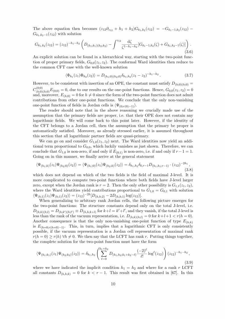
The above equation then becomes (z12∂z12 + h1 + h2)Gk1,k2(z12) = −Gk1−1,k2(z12) −Gk1,k2−1(z12) with solution
Gk1,k2(z12) = (z12)−h1−h2
(D(h1;k1)(h2;k2) −
∫ z12 dζ
ζ1−h1−h2[Gk1−1,k2(ζ) + Gk1,k2−1(ζ)]
).
(3.6)An explicit solution can be found in a hierarchical way, starting with the two-point func-tion of proper primary fields, G0,0(z1, z2). The conformal Ward identities then reduce tothe common CFT case with the well-known solution
However, to be consistent with insertion of an OPE, the constant must satisfy D(h;0)(h;0) =
C(0;0)(h;0)(h;0)E(0;0) = 0, due to our results on the one-point functions. Hence, G0,0(z1, z2) = 0
and, moreover, E(h;0) = 0 for h 6= 0 since the form of the two-point function does not admitcontributions from other one-point functions. We conclude that the only non-vanishingone-point function of fields in Jordan cells is 〈Ψ(0;r(0)−1)〉.
The reader should note that in the above reasoning we crucially made use of theassumption that the primary fields are proper, i.e. that their OPE does not contain anylogarithmic fields. We will come back to this point later. However, if the identity ofthe CFT belongs to a Jordan cell, then the assumption that the primary be proper isautomatically satisfied. Moreover, as already stressed earlier, it is assumed throughoutthis section that all logarithmic partner fields are quasi-primary.
We can go on and consider G1,0(z1, z2) next. The Ward identities now yield an addi-tional term proportional to G0,0, which luckily vanishes as just shown. Therefore, we canconclude that G1,0 is non-zero, if and only if E(0;1) is non-zero, i.e. if and only if r−1 = 1.Going on in this manner, we finally arrive at the general statement
which does not depend on which of the two fields is the field of maximal J-level. It ismore complicated to compute two-point functions where both fields have J-level largerzero, except when the Jordan rank is r = 2. Then the only other possibility is G1,1(z1, z2),where the Ward identities yield contributions proportional to G1,0 = G0,1 with solution〈Ψ(h;1)(z1)Ψ(h;1)(z2)〉 = (z12)−2h[D(h,h;2) − 2D(h,h;1) log(z12)].
When generalizing to arbitrary rank Jordan cells, the following picture emerges forthe two-point functions: The structure constants depend only on the total J-level, i.e.D(h;k)(h;l) = D(h;k′)(h;l′) ≡ D(h,h;k+l) for k+l = k′+l′, and they vanish, if the total J-level isless than the rank of the vacuum representation, i.e. D(h;k)(h;l) = 0 for k+ l+1 < r(h = 0).Another consequence is that the only non-vanishing one-point function of type E(h;k)
is E(h=0;r(h=0)−1). This, in turn, implies that a logarithmic CFT is only consistentlypossible, if the vacuum representation is a Jordan cell representation of maximal rankr(h = 0) ≥ r(h) ∀h 6= 0. We then say that the LCFT has rank r. Putting things together,the complete solution for the two-point function must have the form
〈Ψ(h1;k1)(z1)Ψ(h2;k2)(z2)〉 = δh1,h2
(k1+k2∑`=0
D(h1,h2;k1+k2−`)(−2)`
`!log`(z12)
)(z12)−h1−h2 ,
(3.9)where we have indicated the implicit condition h1 = h2 and where for a rank r LCFTall constants D(h,h;k) = 0 for k < r − 1. This result was first obtained in [67]. In this
10
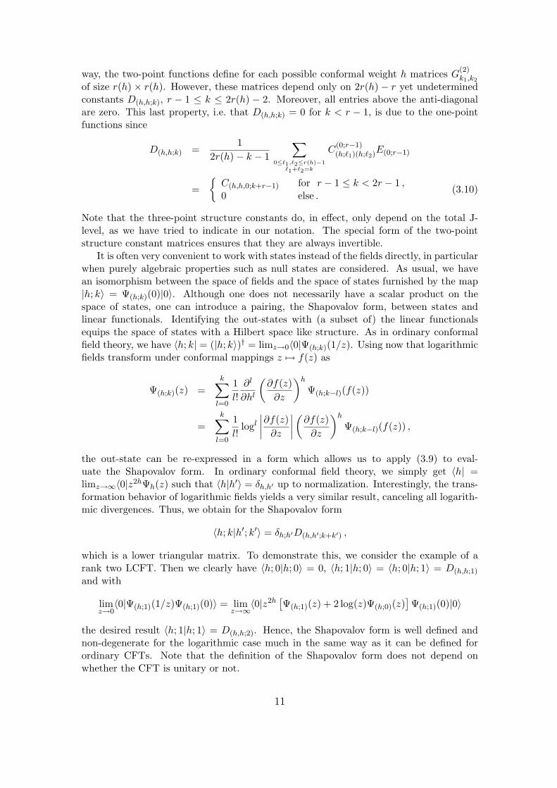
way, the two-point functions define for each possible conformal weight h matrices G(2)k1,k2
of size r(h)× r(h). However, these matrices depend only on 2r(h)− r yet undeterminedconstants D(h,h;k), r − 1 ≤ k ≤ 2r(h) − 2. Moreover, all entries above the anti-diagonalare zero. This last property, i.e. that D(h,h;k) = 0 for k < r − 1, is due to the one-pointfunctions since
D(h,h;k) =1
2r(h)− k − 1
∑0≤`1,`2≤r(h)−1
`1+`2=k
C(0;r−1)(h;`1)(h;`2)E(0;r−1)
={
C(h,h,0;k+r−1) for r − 1 ≤ k < 2r − 1 ,
0 else .(3.10)
Note that the three-point structure constants do, in effect, only depend on the total J-level, as we have tried to indicate in our notation. The special form of the two-pointstructure constant matrices ensures that they are always invertible.
It is often very convenient to work with states instead of the fields directly, in particularwhen purely algebraic properties such as null states are considered. As usual, we havean isomorphism between the space of fields and the space of states furnished by the map|h; k〉 = Ψ(h;k)(0)|0〉. Although one does not necessarily have a scalar product on thespace of states, one can introduce a pairing, the Shapovalov form, between states andlinear functionals. Identifying the out-states with (a subset of) the linear functionalsequips the space of states with a Hilbert space like structure. As in ordinary conformalfield theory, we have 〈h; k| = (|h; k〉)† = limz→0〈0|Ψ(h;k)(1/z). Using now that logarithmicfields transform under conformal mappings z 7→ f(z) as
Ψ(h;k)(z) =k∑
l=0
1l!
∂l
∂hl
(∂f(z)
∂z
)h
Ψ(h;k−l)(f(z))
=k∑
l=0
1l!
logl
∣∣∣∣∂f(z)∂z
∣∣∣∣ (∂f(z)∂z
)h
Ψ(h;k−l)(f(z)) ,
the out-state can be re-expressed in a form which allows us to apply (3.9) to eval-uate the Shapovalov form. In ordinary conformal field theory, we simply get 〈h| =limz→∞〈0|z2hΨh(z) such that 〈h|h′〉 = δh,h′ up to normalization. Interestingly, the trans-formation behavior of logarithmic fields yields a very similar result, canceling all logarith-mic divergences. Thus, we obtain for the Shapovalov form
〈h; k|h′; k′〉 = δh;h′D(h,h′;k+k′) ,
which is a lower triangular matrix. To demonstrate this, we consider the example of arank two LCFT. Then we clearly have 〈h; 0|h; 0〉 = 0, 〈h; 1|h; 0〉 = 〈h; 0|h; 1〉 = D(h,h;1)
and with
limz→0
〈0|Ψ(h;1)(1/z)Ψ(h;1)(0)〉 = limz→∞
〈0|z2h[Ψ(h;1)(z) + 2 log(z)Ψ(h;0)(z)
]Ψ(h;1)(0)|0〉
the desired result 〈h; 1|h; 1〉 = D(h,h;2). Hence, the Shapovalov form is well defined andnon-degenerate for the logarithmic case much in the same way as it can be defined forordinary CFTs. Note that the definition of the Shapovalov form does not depend onwhether the CFT is unitary or not.
11
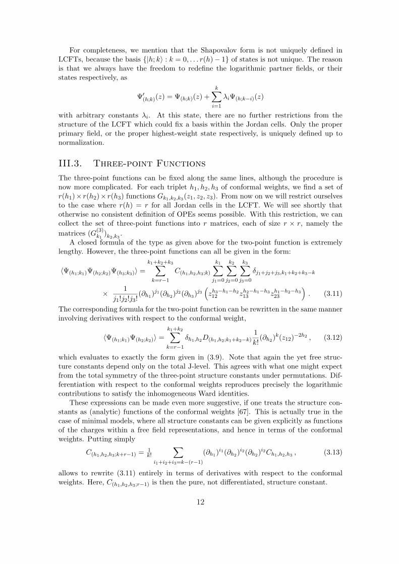
For completeness, we mention that the Shapovalov form is not uniquely defined inLCFTs, because the basis {|h; k〉 : k = 0, . . . r(h)− 1} of states is not unique. The reasonis that we always have the freedom to redefine the logarithmic partner fields, or theirstates respectively, as
Ψ′(h;k)(z) = Ψ(h;k)(z) +
k∑i=1
λiΨ(h;k−i)(z)
with arbitrary constants λi. At this state, there are no further restrictions from thestructure of the LCFT which could fix a basis within the Jordan cells. Only the properprimary field, or the proper highest-weight state respectively, is uniquely defined up tonormalization.
III.3. Three-point Functions
The three-point functions can be fixed along the same lines, although the procedure isnow more complicated. For each triplet h1, h2, h3 of conformal weights, we find a set ofr(h1)× r(h2)× r(h3) functions Gk1,k2,k3(z1, z2, z3). From now on we will restrict ourselvesto the case where r(h) = r for all Jordan cells in the LCFT. We will see shortly thatotherwise no consistent definition of OPEs seems possible. With this restriction, we cancollect the set of three-point functions into r matrices, each of size r × r, namely thematrices (G(3)
k1)k2,k3
.A closed formula of the type as given above for the two-point function is extremely
lengthy. However, the three-point functions can all be given in the form:
〈Ψ(h1;k1)Ψ(h2;k2)Ψ(h3;k3)〉 =k1+k2+k3∑
k=r−1
C(h1,h2,h3;k)
k1∑j1=0
k2∑j2=0
k3∑j3=0
δj1+j2+j3,k1+k2+k3−k
× 1j1!j2!j3!
(∂h1)j1(∂h2)
j2(∂h3)j3(zh3−h1−h212 zh2−h1−h3
13 zh1−h2−h323
). (3.11)
The corresponding formula for the two-point function can be rewritten in the same mannerinvolving derivatives with respect to the conformal weight,
〈Ψ(h1;k1)Ψ(h2;k2)〉 =k1+k2∑k=r−1
δh1,h2D(h1,h2;k1+k2−k)1k!
(∂h2)k(z12)−2h2 , (3.12)
which evaluates to exactly the form given in (3.9). Note that again the yet free struc-ture constants depend only on the total J-level. This agrees with what one might expectfrom the total symmetry of the three-point structure constants under permutations. Dif-ferentiation with respect to the conformal weights reproduces precisely the logarithmiccontributions to satisfy the inhomogeneous Ward identities.
These expressions can be made even more suggestive, if one treats the structure con-stants as (analytic) functions of the conformal weights [67]. This is actually true in thecase of minimal models, where all structure constants can be given explicitly as functionsof the charges within a free field representations, and hence in terms of the conformalweights. Putting simply
C(h1,h2,h3;k+r−1) = 1k!
∑i1+i2+i3=k−(r−1)
(∂h1)i1(∂h2)
i2(∂h2)i2Ch1,h2,h3 , (3.13)
allows to rewrite (3.11) entirely in terms of derivatives with respect to the conformalweights. Here, C(h1,h2,h3;r−1) is then the pure, not differentiated, structure constant.
12
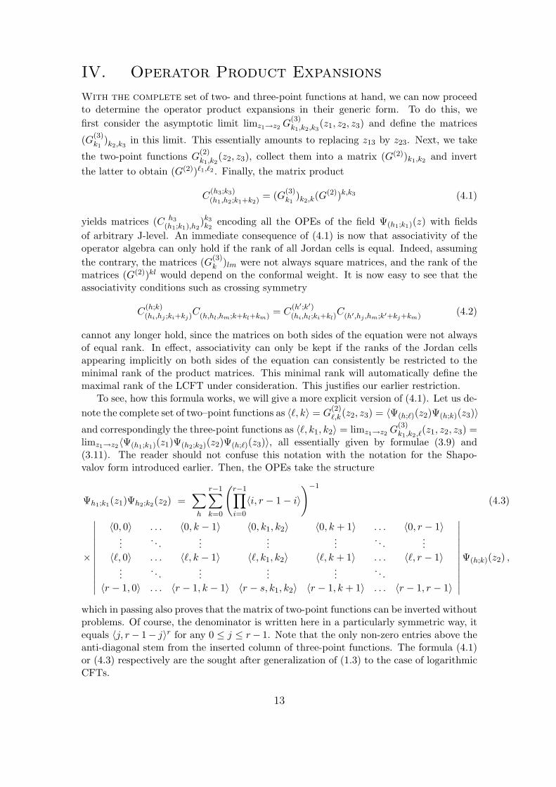
IV. Operator Product Expansions
With the complete set of two- and three-point functions at hand, we can now proceedto determine the operator product expansions in their generic form. To do this, wefirst consider the asymptotic limit limz1→z2 G
(3)k1,k2,k3
(z1, z2, z3) and define the matrices
(G(3)k1
)k2,k3in this limit. This essentially amounts to replacing z13 by z23. Next, we take
the two-point functions G(2)k1,k2
(z2, z3), collect them into a matrix (G(2))k1,k2 and invertthe latter to obtain (G(2))`1,`2 . Finally, the matrix product
C(h3;k3)(h1,h2;k1+k2) = (G(3)
k1)k2,k(G
(2))k,k3 (4.1)
yields matrices (C h3
(h1;k1),h2)k3k2
encoding all the OPEs of the field Ψ(h1;k1)(z) with fieldsof arbitrary J-level. An immediate consequence of (4.1) is now that associativity of theoperator algebra can only hold if the rank of all Jordan cells is equal. Indeed, assumingthe contrary, the matrices (G(3)
k )lm were not always square matrices, and the rank of thematrices (G(2))kl would depend on the conformal weight. It is now easy to see that theassociativity conditions such as crossing symmetry
C(h;k)(hi,hj ;ki+kj)
C(h,hl,hm;k+kl+km) = C(h′;k′)(hi,hl;ki+kl)
C(h′,hj ,hm;k′+kj+km) (4.2)
cannot any longer hold, since the matrices on both sides of the equation were not alwaysof equal rank. In effect, associativity can only be kept if the ranks of the Jordan cellsappearing implicitly on both sides of the equation can consistently be restricted to theminimal rank of the product matrices. This minimal rank will automatically define themaximal rank of the LCFT under consideration. This justifies our earlier restriction.
To see, how this formula works, we will give a more explicit version of (4.1). Let us de-note the complete set of two–point functions as 〈`, k〉 = G
(2)`,k(z2, z3) = 〈Ψ(h;`)(z2)Ψ(h;k)(z3)〉
and correspondingly the three-point functions as 〈`, k1, k2〉 = limz1→z2 G(3)k1,k2,`(z1, z2, z3) =
limz1→z2〈Ψ(h1;k1)(z1)Ψ(h2;k2)(z2)Ψ(h;`)(z3)〉, all essentially given by formulae (3.9) and(3.11). The reader should not confuse this notation with the notation for the Shapo-valov form introduced earlier. Then, the OPEs take the structure
Ψh1;k1(z1)Ψh2;k2(z2) =∑
h
r−1∑k=0
(r−1∏i=0
〈i, r − 1− i〉
)−1
(4.3)
×
∣∣∣∣∣∣∣∣∣∣∣∣
〈0, 0〉 . . . 〈0, k − 1〉 〈0, k1, k2〉 〈0, k + 1〉 . . . 〈0, r − 1〉...
. . ....
......
. . ....
〈`, 0〉 . . . 〈`, k − 1〉 〈`, k1, k2〉 〈`, k + 1〉 . . . 〈`, r − 1〉...
which in passing also proves that the matrix of two-point functions can be inverted withoutproblems. Of course, the denominator is written here in a particularly symmetric way, itequals 〈j, r− 1− j〉r for any 0 ≤ j ≤ r− 1. Note that the only non-zero entries above theanti-diagonal stem from the inserted column of three-point functions. The formula (4.1)or (4.3) respectively are the sought after generalization of (1.3) to the case of logarithmicCFTs.
13
With this result, we obtain in the simplest r = 2 case the well known OPEs
Ψ(h1;0)(z)Ψ(h2;0)(0) =∑
h
C(h1,h2,h;1)
D(h,h;1)
Ψ(h;0)(0)zh−h1−h2 , (4.4)
Ψ(h1;0)(z)Ψ(h2;1)(0) =∑
h
[C(h1,h2,h;1)
D(h,h;1)
Ψ(h;1)(0) (4.5)
+D(h,h;1)C(h1,h2,h;2) −D(h,h;2)C(h1,h2,h;1)
D2(h,h;1)
Ψ(h;0)(0)
]zh−h1−h2 ,
Ψ(h1;1)(z)Ψ(h2;1)(0) =∑
h
[(C(h1,h2,h;2)
D(h,h;1)
−2C(h1,h2,h;1)
D(h,h;1)
log(z)
)Ψ(h;1)(0) (4.6)
+
(D(h,h;1)C(h1,h2,h;3) −D(h,h;2)C(h1,h2,h;2)
D2(h,h;1)
+2D(h,h;2)C(h1,h2,h;1) −D(h,h;1)C(h1,h2,h;2)
D2(h,h;1)
log(z)
−D(h,h;1)C(h1,h2,h;1)
D2(h,h;1)
log2(z)
)Ψ(h;0)(0)
]zh−h1−h2
Note that, for instance, the OPE of a proper primary with its logarithmic partner neces-sarily receives two contributions. One might naively have expected that proper primaryfields do not change the J-level, although already the OPE of the stress-energy tensor witha logarithmic field will have an additional term involving the primary field. At the endof this section we will give a complete non-trivial example, namely the full set of genericOPE forms for a LCFT with rank four Jordan cells.
But before doing so, we want to remark on the question of locality. The two- andthree-point functions and the OPEs can easily be brought into a form for a local LCFTconstructed out of left- and right-chiral half. The rule for this is simply to replace eachlog(zij) by log |zij |2, and to replace each power (zij)µij by |zij |2µij . This yields a LCFTwhere all fields have the same holomorphic and anti-holomorphic scaling dimensions andthe same J-level. Such an ansatz automatically satisfies both, the holomorphic as wellas the anti-holomorphic Ward identities, if z and z are formally treated as independentvariables. It is important to note, however, that the resulting full amplitudes do notfactorize into holomorphic and anti-holomorphic parts. This is a well known feature ofLCFTs. For example, the OPE equation (4.6) would read in its full form
Ψ(h1;1)(z, z)Ψ(h2;1)(0, 0) =∑
h
|z|2(h−h1−h2)
[C(2) − 2C(1) log |z|2
D(1)
Ψ(h;1)(0, 0) (4.7)
+
(D(1)C(3) −D(2)C(2)
D2(1)
+2D(2)C(1) −D(1)C(2)
D2(1)
log |z|2 −D(1)C(1)
D2(1)
log2 |z|2)
Ψ(h;0)(0, 0)
]
with an obvious abbreviation for the structure constants. The reader is encouraged toconvince herself of both, that on one hand this does indeed not factorize into holomorphicand anti-holomorphic parts, but that on the other hand this does satisfy the full set ofconformal Ward identities.
14
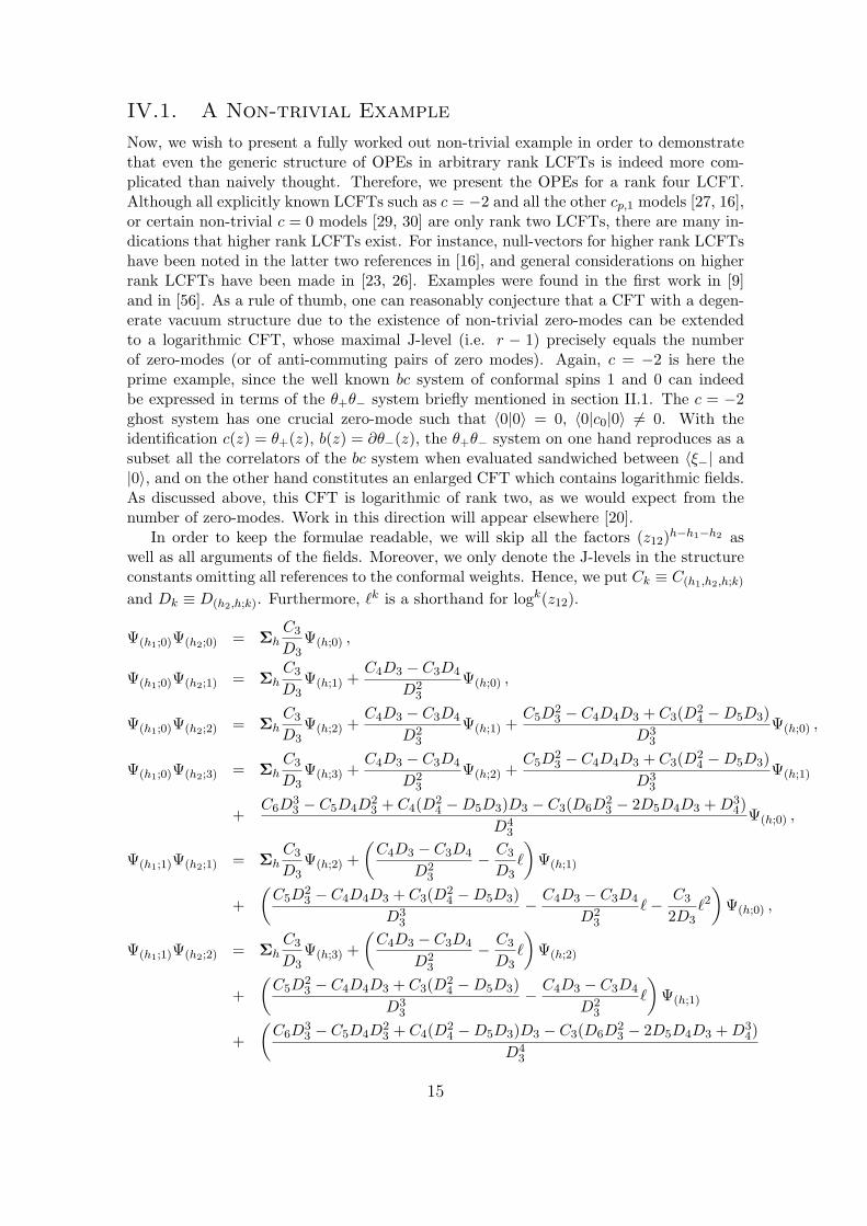
IV.1. A Non-trivial Example
Now, we wish to present a fully worked out non-trivial example in order to demonstratethat even the generic structure of OPEs in arbitrary rank LCFTs is indeed more com-plicated than naively thought. Therefore, we present the OPEs for a rank four LCFT.Although all explicitly known LCFTs such as c = −2 and all the other cp,1 models [27, 16],or certain non-trivial c = 0 models [29, 30] are only rank two LCFTs, there are many in-dications that higher rank LCFTs exist. For instance, null-vectors for higher rank LCFTshave been noted in the latter two references in [16], and general considerations on higherrank LCFTs have been made in [23, 26]. Examples were found in the first work in [9]and in [56]. As a rule of thumb, one can reasonably conjecture that a CFT with a degen-erate vacuum structure due to the existence of non-trivial zero-modes can be extendedto a logarithmic CFT, whose maximal J-level (i.e. r − 1) precisely equals the numberof zero-modes (or of anti-commuting pairs of zero modes). Again, c = −2 is here theprime example, since the well known bc system of conformal spins 1 and 0 can indeedbe expressed in terms of the θ+θ− system briefly mentioned in section II.1. The c = −2ghost system has one crucial zero-mode such that 〈0|0〉 = 0, 〈0|c0|0〉 6= 0. With theidentification c(z) = θ+(z), b(z) = ∂θ−(z), the θ+θ− system on one hand reproduces as asubset all the correlators of the bc system when evaluated sandwiched between 〈ξ−| and|0〉, and on the other hand constitutes an enlarged CFT which contains logarithmic fields.As discussed above, this CFT is logarithmic of rank two, as we would expect from thenumber of zero-modes. Work in this direction will appear elsewhere [20].
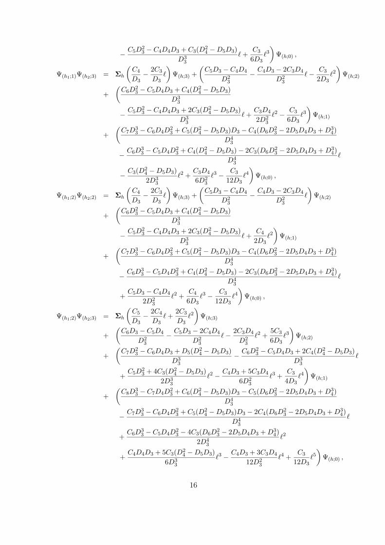
In order to keep the formulae readable, we will skip all the factors (z12)h−h1−h2 aswell as all arguments of the fields. Moreover, we only denote the J-levels in the structureconstants omitting all references to the conformal weights. Hence, we put Ck ≡ C(h1,h2,h;k)
and Dk ≡ D(h2,h;k). Furthermore, `k is a shorthand for logk(z12).
Ψ(h1;0)Ψ(h2;0) = ΣhC3
D3Ψ(h;0) ,
Ψ(h1;0)Ψ(h2;1) = ΣhC3
D3Ψ(h;1) +
C4D3 − C3D4
D23
Ψ(h;0) ,
Ψ(h1;0)Ψ(h2;2) = ΣhC3
D3Ψ(h;2) +
C4D3 − C3D4
D23
Ψ(h;1) +C5D
23 − C4D4D3 + C3(D2
4 −D5D3)D3
3
Ψ(h;0) ,
Ψ(h1;0)Ψ(h2;3) = ΣhC3
D3Ψ(h;3) +
C4D3 − C3D4
D23
Ψ(h;2) +C5D
23 − C4D4D3 + C3(D2
4 −D5D3)D3
3
Ψ(h;1)
+C6D
33 − C5D4D
23 + C4(D2
4 −D5D3)D3 − C3(D6D23 − 2D5D4D3 + D3
4)D4
3
Ψ(h;0) ,
Ψ(h1;1)Ψ(h2;1) = ΣhC3
D3Ψ(h;2) +
(C4D3 − C3D4
D23
− C3
D3`
)Ψ(h;1)
+(
C5D23 − C4D4D3 + C3(D2
4 −D5D3)D3
3
− C4D3 − C3D4
D23
`− C3
2D3`2
)Ψ(h;0) ,
Ψ(h1;1)Ψ(h2;2) = ΣhC3
D3Ψ(h;3) +
(C4D3 − C3D4
D23
− C3
D3`
)Ψ(h;2)
+(
C5D23 − C4D4D3 + C3(D2
4 −D5D3)D3
3
− C4D3 − C3D4
D23
`
)Ψ(h;1)
+(
C6D33 − C5D4D
23 + C4(D2
4 −D5D3)D3 − C3(D6D23 − 2D5D4D3 + D3
4)D4
3
15
− C5D23 − C4D4D3 + C3(D2
4 −D5D3)D3
3
` +C3
6D3`3
)Ψ(h;0) ,
Ψ(h1;1)Ψ(h2;3) = Σh
(C4
D3− 2C3
D3`
)Ψ(h;3) +
(C5D3 − C4D4
D23
− C4D3 − 2C3D4
D23
`− C3
2D3`2
)Ψ(h;2)
+(
C6D23 − C5D4D3 + C4(D2
4 −D5D3)D3
3
− C5D23 − C4D4D3 + 2C3(D2
4 −D5D3)D3
3
` +C3D4
2D23
`2 − C3
6D3`3
)Ψ(h;1)
+(
C7D33 − C6D4D
23 + C5(D2
4 −D5D3)D3 − C4(D6D23 − 2D5D4D3 + D3
4)D4
3
− C6D33 − C5D4D
23 + C4(D2
4 −D5D3)− 2C3(D6D23 − 2D5D4D3 + D3
4)D4
3
`
− C3(D24 −D5D3)2D3
3
`2 +C3D4
6D23
`3 − C3
12D3`4
)Ψ(h;0) ,
Ψ(h1;2)Ψ(h2;2) = Σh
(C4
D3− 2C3
D3`
)Ψ(h;3) +
(C5D3 − C4D4
D23
− C4D3 − 2C3D4
D23
`
)Ψ(h;2)
+(
C6D23 − C5D4D3 + C4(D2
4 −D5D3)D3
3
− C5D23 − C4D4D3 + 2C3(D2
4 −D5D3)D3
3
` +C4
2D3`2
)Ψ(h;1)
+(
C7D33 − C6D4D
23 + C5(D2
4 −D5D3)D3 − C4(D6D23 − 2D5D4D3 + D3
4)D4
3
− C6D33 − C5D4D
23 + C4(D2
4 −D5D3)− 2C3(D6D23 − 2D5D4D3 + D3
4)D4
3
`
+C5D3 − C4D4
2D23
`2 +C4
6D3`3 − C3
12D3`4
)Ψ(h;0) ,
Ψ(h1;2)Ψ(h2;3) = Σh
(C5
D3− 2C4
D3` +
2C3
D3`2
)Ψ(h;3)
+(
C6D3 − C5D4
D23
− C5D3 − 2C4D4
D23
`− 2C3D4
D23
`2 +5C3
6D3`3
)Ψ(h;2)
+(
C7D23 − C6D4D3 + D5(D2
4 −D5D3)D3
3
− C6D23 − C5D4D3 + 2C4(D2
4 −D5D3)D3
3
`
+C5D
23 + 4C3(D2
4 −D5D3)2D3
3
`2 − C4D3 + 5C3D4
6D23
`3 +C3
4D3`4
)Ψ(h;1)
+(
C8D33 − C7D4D
23 + C6(D2
4 −D5D3)D3 − C5(D6D23 − 2D5D4D3 + D3
4)D4
3
− C7D33 − C6D4D
23 + C5(D2
4 −D5D3)D3 − 2C4(D6D23 − 2D5D4D3 + D3
4)D4
3
`
+C6D
33 − C5D4D
23 − 4C3(D6D
23 − 2D5D4D3 + D3
4)2D4
3
`2
+C4D4D3 + 5C3(D2
4 −D5D3)6D3
3
`3 − C4D3 + 3C3D4
12D23
`4 +C3
12D3`5
)Ψ(h;0) ,
16
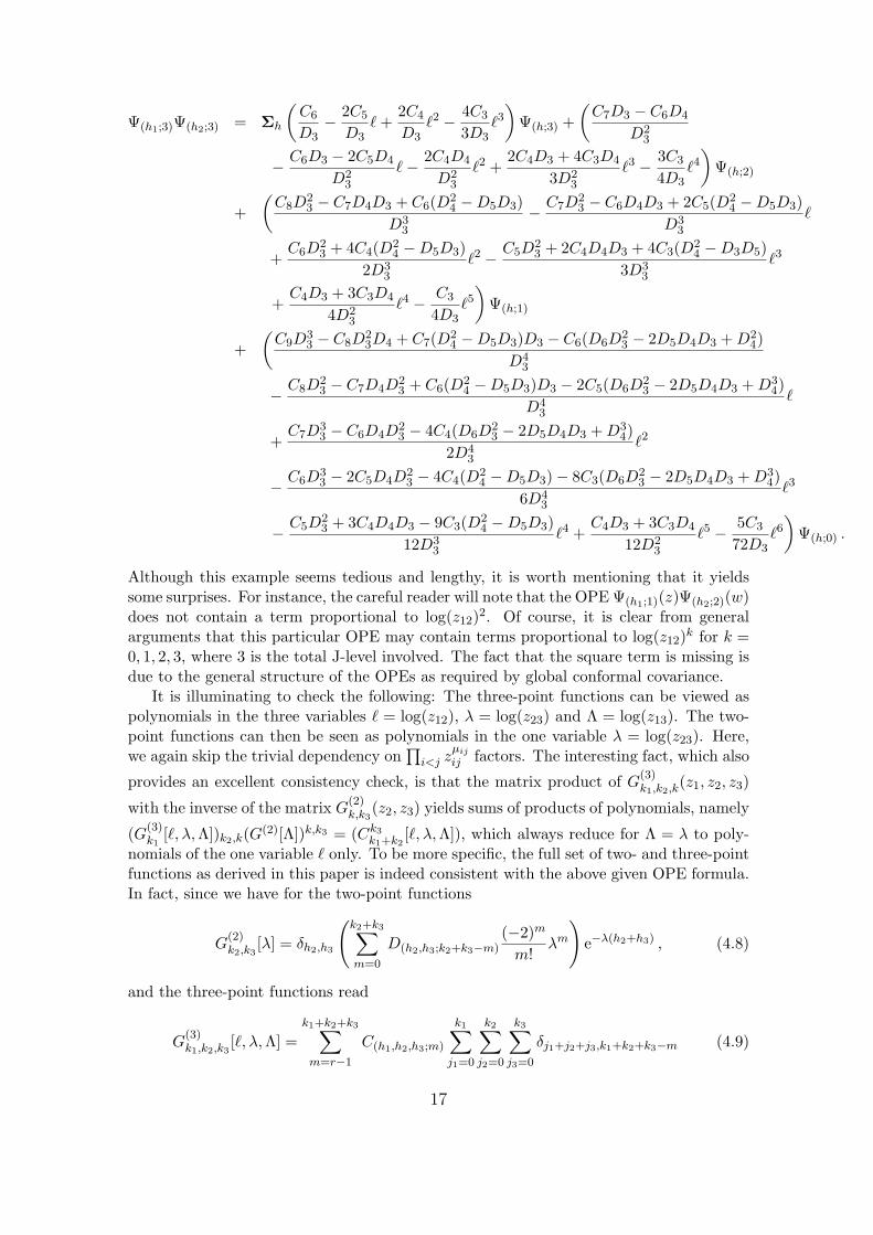
Ψ(h1;3)Ψ(h2;3) = Σh
(C6
D3− 2C5
D3` +
2C4
D3`2 − 4C3
3D3`3
)Ψ(h;3) +
(C7D3 − C6D4
D23
− C6D3 − 2C5D4
D23
`− 2C4D4
D23
`2 +2C4D3 + 4C3D4
3D23
`3 − 3C3
4D3`4
)Ψ(h;2)
+(
C8D23 − C7D4D3 + C6(D2
4 −D5D3)D3
3
− C7D23 − C6D4D3 + 2C5(D2
4 −D5D3)D3
3
`
+C6D
23 + 4C4(D2
4 −D5D3)2D3
3
`2 − C5D23 + 2C4D4D3 + 4C3(D2
4 −D3D5)3D3
3
`3
+C4D3 + 3C3D4
4D23
`4 − C3
4D3`5
)Ψ(h;1)
+(
C9D33 − C8D
23D4 + C7(D2
4 −D5D3)D3 − C6(D6D23 − 2D5D4D3 + D2
4)D4
3
− C8D23 − C7D4D
23 + C6(D2
4 −D5D3)D3 − 2C5(D6D23 − 2D5D4D3 + D3
4)D4
3
`
+C7D
33 − C6D4D
23 − 4C4(D6D
23 − 2D5D4D3 + D3
4)2D4
3
`2
− C6D33 − 2C5D4D
23 − 4C4(D2
4 −D5D3)− 8C3(D6D23 − 2D5D4D3 + D3
4)6D4
3
`3
− C5D23 + 3C4D4D3 − 9C3(D2
4 −D5D3)12D3
3
`4 +C4D3 + 3C3D4
12D23
`5 − 5C3
72D3`6
)Ψ(h;0) .
Although this example seems tedious and lengthy, it is worth mentioning that it yieldssome surprises. For instance, the careful reader will note that the OPE Ψ(h1;1)(z)Ψ(h2;2)(w)does not contain a term proportional to log(z12)2. Of course, it is clear from generalarguments that this particular OPE may contain terms proportional to log(z12)k for k =0, 1, 2, 3, where 3 is the total J-level involved. The fact that the square term is missing isdue to the general structure of the OPEs as required by global conformal covariance.
It is illuminating to check the following: The three-point functions can be viewed aspolynomials in the three variables ` = log(z12), λ = log(z23) and Λ = log(z13). The two-point functions can then be seen as polynomials in the one variable λ = log(z23). Here,we again skip the trivial dependency on
∏i<j z
µij
ij factors. The interesting fact, which also
provides an excellent consistency check, is that the matrix product of G(3)k1,k2,k(z1, z2, z3)
with the inverse of the matrix G(2)k,k3
(z2, z3) yields sums of products of polynomials, namely
(G(3)k1
[`, λ, Λ])k2,k(G(2)[Λ])k,k3 = (Ck3k1+k2
[`, λ, Λ]), which always reduce for Λ = λ to poly-nomials of the one variable ` only. To be more specific, the full set of two- and three-pointfunctions as derived in this paper is indeed consistent with the above given OPE formula.In fact, since we have for the two-point functions
G(2)k2,k3
[λ] = δh2,h3
(k2+k3∑m=0
D(h2,h3;k2+k3−m)(−2)m
m!λm
)e−λ(h2+h3) , (4.8)
and the three-point functions read
G(3)k1,k2,k3
[`, λ, Λ] =k1+k2+k3∑m=r−1
C(h1,h2,h3;m)
k1∑j1=0
k2∑j2=0
k3∑j3=0
δj1+j2+j3,k1+k2+k3−m (4.9)
17
× 1j1!j2!j3!
(∂h1)j1(∂h2)
j2(∂h3)j3(e`(h3−h1−h2)eΛ(h2−h1−h3)eλ(h1−h2−h3)
),
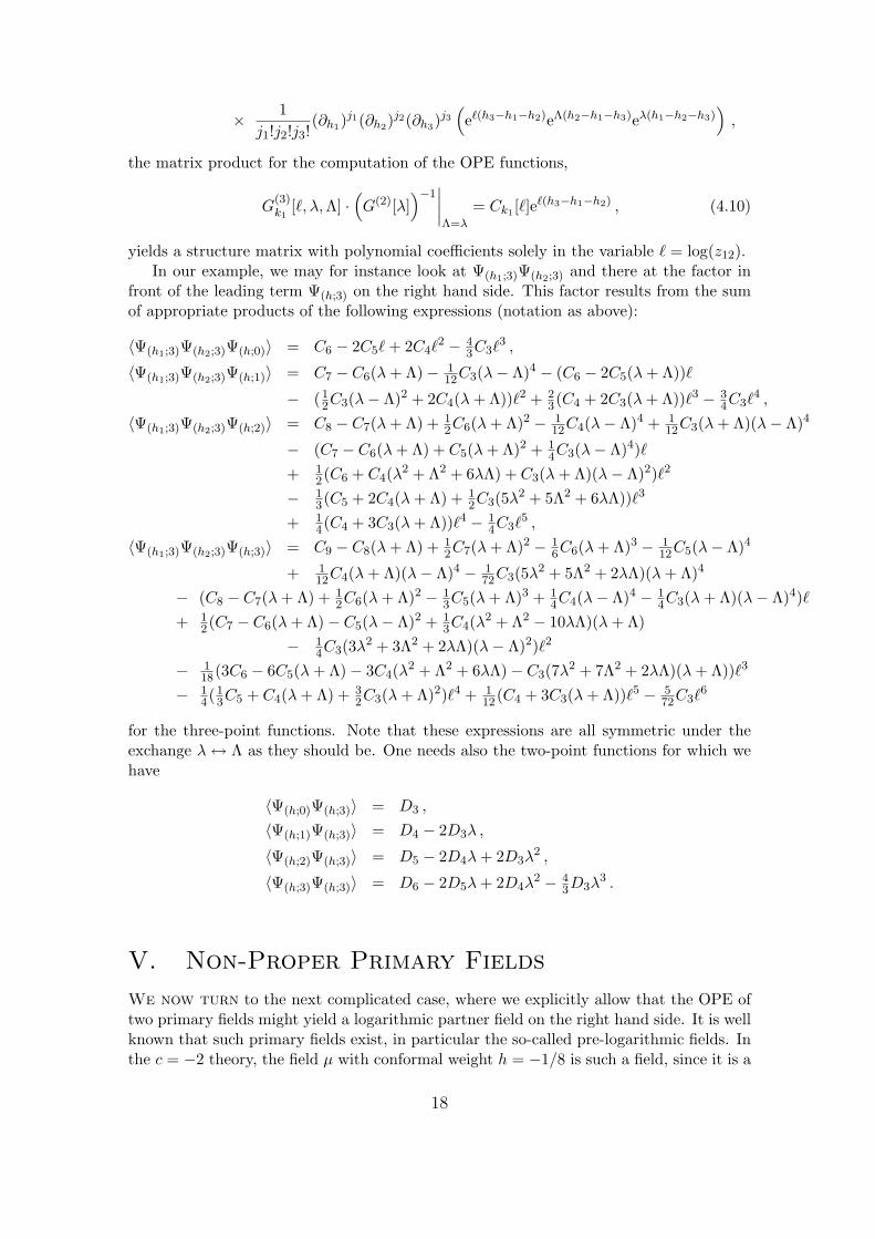
the matrix product for the computation of the OPE functions,
G(3)k1
[`, λ, Λ] ·(G(2)[λ]
)−1∣∣∣∣Λ=λ
= Ck1 [`]e`(h3−h1−h2) , (4.10)
yields a structure matrix with polynomial coefficients solely in the variable ` = log(z12).In our example, we may for instance look at Ψ(h1;3)Ψ(h2;3) and there at the factor in
front of the leading term Ψ(h;3) on the right hand side. This factor results from the sumof appropriate products of the following expressions (notation as above):
for the three-point functions. Note that these expressions are all symmetric under theexchange λ ↔ Λ as they should be. One needs also the two-point functions for which wehave
〈Ψ(h;0)Ψ(h;3)〉 = D3 ,
〈Ψ(h;1)Ψ(h;3)〉 = D4 − 2D3λ ,
〈Ψ(h;2)Ψ(h;3)〉 = D5 − 2D4λ + 2D3λ2 ,
〈Ψ(h;3)Ψ(h;3)〉 = D6 − 2D5λ + 2D4λ2 − 4
3D3λ3 .
V. Non-Proper Primary Fields
We now turn to the next complicated case, where we explicitly allow that the OPE oftwo primary fields might yield a logarithmic partner field on the right hand side. It is wellknown that such primary fields exist, in particular the so-called pre-logarithmic fields. Inthe c = −2 theory, the field µ with conformal weight h = −1/8 is such a field, since it is a
18
Virasoro primary field with OPE µ(z)µ(w) = (z − w)1/4(I(w)− 2 log(z − w)I). However,the primary field µ is not itself part of a Jordan cell. The c = −2 theory provides anotherexample of primary fields whose OPE also yields the field I, namely the so-called fermionicfields θα. With our notation introduced in section II.1, the former pre-logarithmic fieldsare twist fields, i.e. fields with non-trivial boundary conditions. Such fields do not have azero mode content. The latter fields, however, have a zero mode content with the propertythat Z+(θα) 6= Z−(θα), since Zβ(θα) = δαβ . These fields are again not members of Jordancells.
Of course, one might imagine a situation where non-proper primary fields do formpart of a Jordan cell. The problem then is, that it is no longer possible to solve theconformal Ward identities in a hierarchical manner, as in section III, without furtherknowledge about the operator algebra. Basically, our approach in the third section wasto find the first non-vanishing two- and three-point functions, the ones with minimal zeromode content, and to derive correlators with higher zero-mode content by solving theinhomogeneous Ward identities step by step. If the zero mode content of all fields isknown, we can estimate which two- and three-point functions might be non-zero, sincethe OPE must satisfy the bound
Z0(Ψ3) ≤ Z0(Ψ1) + Z0(Ψ2) (5.11)
for all fields Ψ3(w) in the operator product of Ψ1(z) with Ψ2(w). This would provide uswith a starting point for the hierarchical solution scheme. Unfortunately, this does notwork for the twist fields, because no zero mode content can be defined for them. There isso far no example known where twist fields form part of a Jordan cell. We don’t see aneasy way to extend our description of Jordan cells in terms of zero mode content of fieldssuch that it would encompass twist fields within Jordan cells. Thus we leave investigationof this case for future work.
V.1. Fermionic Fields
Let us now concentrate on the best known case of a rank r = 2 LCFT, i.e. where themaximal rank of Jordan cells is two, as in the prime example of the c = −2 theory.There, logarithmic operators, which together with their proper primary partners span theJordan cells, are created by the operator I(z) = Ψ(0;1)(z). As long as no twist fields areconsidered, we can construct all fields in terms of the pair of anti-commuting scalar θfields defined in section II.1. Remember that the ξ modes become the creation operatorsfor logarithmic states. It is easy to see that proper primary fields do not possess any ofthe ξ zero modes, while logarithmic fields possess precisely the zero mode contribution12εαβξαξβ. Since the ξ modes do anti-commute, we call fields with just one ξ zero modefermionic, and fields which are quadratic in ξ bosonic. This coincides with the fact that forc = −2 all logarithmic fields and all proper primary fields have integer conformal weights.However, nothing prohibits us from considering the fields θα(z) themselves which alsohave zero conformal weight, but are fermionic. Many of the above arguments remainvalid when we consider correlation functions involving θ fields. A further restriction isthat the total number of θ fields must be even, since otherwise the correlation functionvanishes identically. The reason is that consistency with the anti-commutation relationsenforces to put 〈ξ+〉 = 〈ξ−〉 = 0. Only when the total number of θ fields is even, do wehave a chance that a term ξ+ξ− will survive after contraction. Moreover, the number ofθ+ and θ− fields must be equal, since otherwise θ±,0 zero modes will survive.
19
More generally, a correlator of fields 〈Ψ1(z1) . . .Ψn(zn)〉 can only be non-zero, if itsatisfies the conditions∑
i
Z+(Ψi) =∑
i
Z−(Ψi) and∑
i
Z0(Ψi) ≥ 2 (5.12)
in the rank two case. This statement is valid for fields Ψi which are either proper primaries,logarithmic partners or fermionic fields (i.e. fields with fermionic zero mode content).
Correlation functions involving fermionic fields can be computed along the same linesas set out above. The only difference is that the action of the Virasoro algebra on fermionicfields does not have an off-diagonal part in the rank two case. More precisely, this is truefor the L0 mode of the Virasoro algebra, since this mode reduces always the total zeromode content symmetrically, i.e. it reduces Z− by the same amount as Z+. Other modes,such as L1, can reduce the zero mode content unevenly, as we will see in the next section.As long as we still assume that all fields in a Jordan cell are quasi-primary, we don’t haveto worry about this possibility. Of course, in LCFTs of higher rank, fermionic fields caneasily admit an off-diagonal action of L0, since Z± can both be larger than one. To keepthe following formulæ reasonable simple, we won’t consider this case here.
The important fact is that the OPE of two fermionic fields produces a logarithm, i.e.
θα(z)θβ(0) = εαβ
(I(0) + (1 + log z)I(0)
). (5.13)
This follows on general grounds, since 〈θα(z)θβ(w)〉 = εαβ such that a three-point functionof two fermionic and one logarithmic field necessarily involves a logarithm. The argumentremains valid in the general rank two case and fields of arbitrary scaling dimension. EachJordan cell is extended by two fermionic sectors such that we have the four fields Ψ(h;0),Ψ(h;1), and Ψ(h;±). It is then an easy task to compute all their OPEs from the two- andthree-point functions
and permutations. Note that we have explicitly indicated the antisymmetry under ex-changing the order of the fermionic fields. These results agree in the special case where allhi = 0 with the explicit calculations for the c = −2 LCFT by Kausch [34]. The singularterms of the corresponding additional OPEs read
The above statement shows that rank two LCFTs naturally allow for fermionic fields. Ithas been suggested in [61] to formally collect these quadruples of fields in “superfields”Ψh(z, η+, η−) of N =2 Grassmann variables such that
which in the c = −2 case resembles the ξ± zero mode contributions. It is tempting toconjecture that a rank k LCFT will naturally incorporate the analog of anti-commutingscalars for Zk para-fermions, whose OPEs among them create logarithmic fields of ac-cording J-levels. However, an investigation of this is beyond the scope of the presentpaper.
V.2. Twist Fields
As already explained, there is (at least) one more sort of fields which may occur in LCFTs.In the standard c = −2 example, the two fields µ(z) and σ(z) with conformal weightshµ = −1/8 and hσ = 3/8 respectively, are not yet accounted for. These fields are twistfields. They can be treated much along the same lines as fermionic fields. The difference isthat their mode expansion is in Z+ ι with a certain rational ι depending on the boundaryconditions and the ramification number of the twists. The fields µ and σ are Z2 twists.Despite the difference in the mode expansion, twist fields behave quite similar to the(para-)fermionic fields mentioned above. In particular, their two-point functions are non-zero if and only if they involve a twist χι and its anti-twist χι∗ , which resembles the factthat for fermionic fields only the two-point function of two different fermions is non-zero.Higher twist fields are then analogous to para-fermions.
One might attempt to extend the definition of zero mode content to rational numberssuch that a twist field with mode expansion in Z+ι would get assigned Z0(χι) = Z+(χι)+Z−(χι) = ι + ι∗. A necessary condition for a correlator 〈χι1 . . . χιn〉 to be non-zero wouldthen read ∑
i
Z+(χιi) ∈ Z and∑
i
Z−(χιi) ∈ Z . (5.16)
However, such an assignment is obviously only determined modulo integers, and it is nota priory clear how to implement the condition for a minimal zero mode content in general.At least, one should now always consider separately the zero mode content Z+ and Z−,as indicated above. In the rank two case, however, we can incorporate the condition for aminimal zero mode content into (5.16) by simply replacing Z by N. Indeed, the Z2 twistfields µ and σ have twist numbers (ι, ι∗) = (1
2 , 12) and (−1
2 , 32) respectively, from which we
immediately can read off, which two- and three-point functions of µ and σ fields can benon-zero.
To emphasize the common features of fermionic and twist fields, we contrast theirpossible two- and three-point functions with the ones for fermionic fields (there are no
21
non-vanishing two- or three-point functions involving both, fermionic and twist fields,simultaneously). The notation ι∗ means the anti-twist 1 − ι with respect to ι, and onealways has hι = hι∗ . The only nontrivial two-point function then reads
〈χι(z1)χι∗(z2)〉 = Dιι∗(z12)−2hι (5.17)
with Dιι∗ = Dι∗ι. Note that in contrast to the fermionic fields, twist fields are symmetric.The three-point functions are easily computed and the results are
Note that some of the introduced constants may be zero, e.g. Cι1ι2ι3 = 0 whenever thethree twists do not add up to an integer. Most remarkably is perhaps the fact that〈Ψ(h1;1)Ψ(h2;1)χι3〉 might be non-zero. This does not happen in the c = −2 theory, sinceit implies that the OPE of two logarithmic fields has a contribution
Ψ(h;1)(z)Ψ(h′;1)(0) = . . . +C(h,h′;2)ι
Dιι∗zhι−h−h′χι(0) + . . . , (5.18)
which is not the case in the c = −2 theory. However, already the next theory in the cp,1
series of LCFTs, namely the c3,1 = −7 model, shows precisely this feature, where thefusion rule of the h = 0 logarithmic field with itself involves the twist field with h = −1
3on the right hand side. Since the main focus of this paper lies on logarithmic fields, wewill not go into further detail here. The OPEs involving χι fields read correspondingly
Ψ(h;0)(z)χι(0) =C(h;0)ιι′
Dιι∗zhι′−hι−hχι′(0) ,
Ψ(h;1)(z)χι(0) =C(h,h′;2)ι
D(h;1)zh′−h−hιΨ(h′;0)
+C(h;1)ιι′ − C(h;0)ιι′ log z
Dιι∗zhι′−hι−hχι′(0) +
C(h;1)ιι′∗
Dιι∗zhι′∗−hι−hχι′∗(0) ,
χι(z)χι′(0) =C(h;1)ιι′
D(h;1)zh′−hι−hι′Ψ(h;0)(0) +
Cιι′ι′′
Dιι∗zhι′′−hι−hι′χι′′(0) ,
χι(z)χι∗(0) =C(h;1)ιι∗D(h;1) − C(h;0)ιι∗D(h;2) + C(h;0)ιι∗D(h;1) log z
D2(h;1)
zh−hι−hι∗Ψ(h;0)(0)
+C(h;0)ιι∗
D(h;1)zh−hι−hι∗Ψ(h;1)(0) ,
where in the last two equations ι′ 6= ι∗. As remarked above, some of the structureconstants may vanish, as they do in the c = −2 LCFT. One sees that even the simplerank two case gets quite complicated and needs a cumbersome notation. The situation isslightly better in the particular case for the c = −2 theory where all amplitudes involvingup to four twist fields as well as amplitudes with an arbitrary number of fermionic fieldswere computed in [34].
22
VI. Non-quasi-primary fields
Our discussion of correlation functions and operator product expansions in logarithmicCFTs heavily relies on the following assumption which we so far have made: that alllogarithmic partner fields within a Jordan cell be quasi-primary. This means in particularthat L1|h; k〉 = L1Φ(h;k)(0)|0〉 = 0. As a consequence, we could make elaborate use ofthe Ward identities of global conformal transformations in the form (3.2). This section isdevoted to the question under which more relaxed circumstances our results still hold.
It is by no means clear that logarithmic partner fields are indeed all quasi-primary.On the contrary, even the simplest known LCFT, the c = −2 model, features a Jordancell where the logarithmic partner is not quasi-primary [21]. Actually, as already outlinedin section II, in this model exists a Jordan cell for conformal weight h = 1, built froma primary field† ∂θα(z) and its logarithmic partner field :θ+θ−∂θα:(z). Here, we againused the realization of the c = −2 theory in terms of two anti-commuting scalar fieldsθ±(z) along the lines (2.10) and (2.11). It is easy to see that |1; 0〉 = θα,−1|0〉 and that|1; 1〉 = θα,−1(ξ+ξ−+1)|0〉. It follows that L1|1; 0〉 = 0, while L1|1; 1〉 = −ξα|0〉 6= 0, whereone uses that the stress-energy tensor is given by (2.9). We remind the reader that ξα isone of the two zero-modes of the field θα(z). Hence, |1; 1〉 is not a state corresponding toa quasi-primary field.
The point is that it does not matter. The global Ward identities are not affected bythis non-zero term. More generally, all correlation functions involving the field Ψ(h=1;1)(z),the logarithmic partner of the primary h = 1 field Ψ(h=1;0)(z) = ∂θ(z), behave exactlyas if the field were quasi-primary. The reason for this is simply that the state L1|1; 1〉 isfermionic with respect to the number of ξα zero modes. More precisely, it has Z+ = 1,Z− = 0 (or vice versa). Any correlation function can only be non-zero if the numbers(Z+, Z−) of ξ± zero modes are, after all contractions are done, exactly (1, 1). Hence, anycorrelation function involving Ψ(h=1;1)(z), which has a chance to be non-zero, must initiallyhave fermion numbers (Z+, Z−) with Z+ + Z− even and Z+ ≥ 1, Z− ≥ 1. Applying L1
to it results in the global conformal Ward identity up to additional terms with fermionnumbers (Z+ − 1, Z−) or (Z+, Z− − 1). Since Z+ + Z− − 1 is then necessarily an oddnumber, the additional terms must vanish. It follows that the fact that Ψ(h=1;1)(z) isnot quasi-primary does not influence the correlation functions, because the spoiling termdoes not lead to any non-vanishing contributions. Note that this statement is only trueas long as we consider the effect within correlation functions. The deeper reason is thatthe action of the Virasoro algebra changes the fermion numbers unevenly in this case.
Of course, not all correlation functions involving a field θα(z) corresponding to thestate ξα|0〉 automatically vanish. For example, 〈0|θ+(z)θ−(w)|0〉 6= 0. What is meant inthe above discussion is that all correlation functions vanish, which result from applyingL1 to a correlator involving Ψ(h=1;1)(z) and other fields such that the initial correlatormight be non-zero. Since L1 acts as a derivation, it only changes one of the inserted fieldsat a time, so that starting with an admissible number of ξα zero modes leads to termswith non-admissible numbers of ξα zero modes.
There are strong indications that this structure of Jordan cells with non-quasi-primaryfields is more generally true. At least, there is so far no LCFT explicitly known wherelogarithmic partner fields are not quasi-primary in a way which would affect correlationfunctions and therefore our general conclusions on their general structure. All LCFTs
†More precisely, we are dealing with a doublet of two such fields, distinguished by the α-label.
23
which can be constructed or realized explicitly in terms of fundamental free fields, such asthe c = −2 model, receive their peculiar logarithmic fields ultimately due to the existenceof conjugate pairs of zero-modes. In the c = −2 model, these are the two pairs ξ±, θ∓,0
respectively (see sect. II.1). In this situation, we only need that the logarithmic partnerfields are quasi-primary up to terms with the “wrong” number of such zero modes. Here,wrong means in the above explained sense that the number of zero modes gets changedunevenly.
Following the lines of [61], the effective zero mode content is equivalently describedin terms of nilpotent variables with which the fields spanning a Jordan cell are groupedtogether in a superfield like fashion. In the rank two case this is easily accomplishedby introducing for each Jordan cell two Grassmann variables η± and a bosonic nilpotentvariable Θ = η+η− with the property Θ2 = 0. Then, we may group together all fields, theprimary Ψ(h;0)(z), its logarithmic partner Ψ(h;1)(z) and the two fermionic fields Ψ(h;±)(z)as Ψh(z) = Ψ(h;0)(z)+η+Ψ(h;+)(z)+η−Ψ(h;−)(z)+η+η−Ψ(h;1)(z). For higher rank Jordancells, an analogous procedure applies. For a Jordan cell of even rank 2r one needs r−1 pairsof Grassmann variables. The member of J-level k in the Jordan cell itself is given by theelementary completely symmetric polynomial σk(Θ1, . . . ,Θr−1) = σk(η+
1 η−1 , . . . , η+r−1η
−r−1)
of total degree 2k in the η’s. So the primary field Φ(h;0)(z) belongs to σ0 ≡ 1, while the topJ-level field Φ(h;r−1)(z) belongs to σr−1 ∝ η+
1 η+1 . . . η+
r−1η−r−1. The elementary completely
symmetric polynomial σk(x1, . . . , xn) is defined as σk =∑
i1<i2<...ikxi1xi2 . . . xik up to
normalization. Other polynomials p({η±i }), whose monomials m{i} =∏
k ηαkik
have differ-ing partial degrees degη+
j(m{i}) 6= degη−j
(m{i}) for at least one j, belong to fields whichare the higher rank analogons of the fermionic fields described above. Overall symmetryin the Grassmann variables demands that all polynomials must be symmetric polynomialsin the η’s. However, what may be varied is how the total degree is split into η+ variablesand η− variables. Hence, we use the symmetric polynomials in two colors, σl,k−l
k , instead.These can be written as σl,k−l
k ({η+, η−}) = σmax(l,k−l)({Θ})σmin(l,k−l)({ηαmin(l,k−l)}). Note
that σl,k−lk = 0 for l or k − l larger r − 1. The Jordan cell is then spanned by the fields
corresponding to the symmetric polynomials σk,k2k ({η+, η+}) = σk({Θ}).
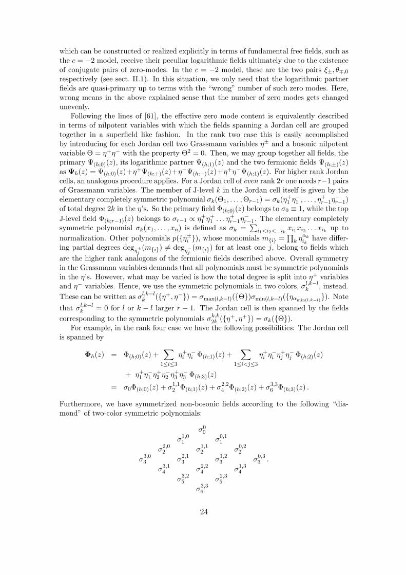
For example, in the rank four case we have the following possibilities: The Jordan cellis spanned by
Φh(z) = Φ(h;0)(z) +∑
1≤i≤3
η+i η−i Φ(h;1)(z) +
∑1≤i<j≤3
η+i η−i η+
j η−j Φ(h;2)(z)
+ η+1 η−1 η+
2 η−2 η+3 η−3 Φ(h;3)(z)
= σ0Φ(h;0)(z) + σ1,12 Φ(h;1)(z) + σ2,2
4 Φ(h;2)(z) + σ3,36 Φ(h;3)(z) .
Furthermore, we have symmetrized non-bosonic fields according to the following “dia-mond” of two-color symmetric polynomials:
σ00
σ1,01 σ0,1
1
σ2,02 σ1,1
2 σ0,22
σ3,03 σ2,1
3 σ1,23 σ0,3
3 .
σ3,14 σ2,2
4 σ1,34
σ3,25 σ2,3
5
σ3,36
24
Of course, it is not clear whether all higher rank LCFTs fall into this pattern, but thecrucial role of conjugate zero mode pairs suggests so.
It is now easy to see, which correlation functions may be non-zero. Clearly, eachinserted field Φ comes with an associated polynomial σ. Consequently, an arbitrary n-point function can only be non-vanishing, if the product
∏ni=1 σli,ki−li
kimeets the conditions
n∑i=1
li =n∑
i=1
(ki − li) ≥ r − 1 . (6.1)
Of course, this is nothing else than our initial conditions on the zero mode content, sinceany field with associated polynomial σl,k−l
k has zero mode content Z+ = l, Z− = k − l.The action of symmetry generators such as the modes of the Virasoro algebra may have
off-diagonal contributions meaning that they change a field into another and thus changea given associated polynomial into another. However, this off-diagonal term contributesto the correlator only if the resulting product of associated polynomials again satisfies theabove condition (6.1). Now, symmetry generators always act as derivations on correlatorssuch that an immediate necessary condition on an off-diagonal term is that the off-diagonalaction of the generator moves vertically in the σ-diamond. Otherwise, the off-diagonalterm has no effect in the correlator. Coming back to our initial example in the c = −2theory, we have that |1; 1〉 has associated polynomial σ1,1
2 , while L1|1; 1〉 has associatedpolynomial σ1,0
1 . Thus, L1 does not move vertically in the σ-diamond, and the non-quasi-primary term hence does not contribute.
We therefore arrive at the following generalized picture: The action of symmetry gen-erators such as the Virasoro algebra in a logarithmic CFT possesses off-diagonal additionalterms with accompanying moves in the associated σ-diamond. However, all such termswith a non-vertical move are irrelevant when considered within correlation functions. Allmoves in the σ-diamond are obviously generated by the two basic moves
Q+ : σl,k−lk 7→ σl,k−1−l
k−1 and Q− : σl,k−lk 7→ σl−1,k−l
k−1 . (6.2)
The careful reader might notice that these moves always go upwards within the diamond.However, since symmetry generators are presumably free of zero modes which do notannihilate the vacuum (otherwise, the vacuum is no longer invariant under the consideredsymmetry), we do not expect that a symmetry generator will move downwards within thediamond. These two basic moves may be viewed as generating a BRST like symmetry,since with 〈
∏i σ
li,ki−liki
〉 6= 0, we certainly have
Q+〈∏
i
σli,ki−liki
〉 =∑
j
〈σl1,k1−l1k1
. . . σlj ,kj−1−ljkj−1 . . . σln,kn−ln
kn〉 = 0 , (6.3)
and analogously for Q−. Actually, one may introduce operators Q±` with 1 ≤ ` ≤ r − 1
which act by setting η∓` formally to one by contracting with a conjugate Grassmannvariable, i.e. by acting with {η∓` , ·}. These latter operators have the nice property toautomatically satisfy (Q±
` )2 = 0, while Q+` Q−
` 6= 0. These latter operators may thenindeed be considered as BRST symmetries on correlation functions. We introduce Q± assymbols for classes of such symmetries, denoting arbitrary moves upwards in the diamond,which are not vertical. Thus, these classes contain also products such as Q+
`1Q+
`2etc.
We may thus finally generalize our assumptions on the fields in LCFTs such that theaction of the Virasoro algebra only needs to satisfy our basic conditions (3.1) and (3.2) up
25
to terms, which can be written as Q± of an admissible configuration, i.e. can be writtenas Q±〈
∏i σ
li,ki−liki
〉 with 〈∏
i σli,ki−liki
〉 satisfying (6.1). If this is the case, all our resultson two- and three-point functions and on the OPE structure remain valid in precisely theform as we have given them. All explicitly known LCFTs seem to possess only Jordancells (and associated non-bosonic fields) which fall into this pattern. However, we do nothave a proof that this has always to be the case. The strongest indications in favor ofsuch a conjecture stem from the classification of possible Jordan structure like modules inthe representation theory of the Virasoro algebra as given in [72]. A deeper study, whichalso should consider Jordan cell structures with respect to other chiral symmetries has tobe left for future work.
Last but not least, we remark that the zero mode content further implies (2.17) andhence (2.16). Let us momentarily assume that these bounds would not be strict. Then,for example, a two-point function 〈Ψ(h;0)(z)Ψ(h;0)(w)〉 could be non-zero, if the OPE ofthe primary field Ψ(h;0) with itself contained Ψ(0;r−1) in the rank r case. It is an easy taskto check that this is, however, inconsistent, since no solution for, say, 〈Ψ(h;1)(z)Ψ(h;0)(w)〉can be found that satisfies all three Ward identities (3.2). On the other hand, two-pointfunctions are insensitive to non-quasi-primary contributions, since these always would re-sult in a two-point function of fields of differing conformal weights. Similar inconsistenciesappear when other cases violating (2.16) are considered.
The higher rank case is more complicated, since OPEs might yield terms of too highJ-level k, which do not influence the two-point functions as long as k < r − 1. Onehas to consider three-point functions: Assume that e.g. the OPE Ψ(h1;0)Ψ(h2;0) producesa term of maximal J-level k with conformal weight h3. Consider 〈Ψ(h1;0)Ψ(h2,0)Ψ(h3,l)〉with l being the minimal J-level such that this three-point function is non-zero, and thushas the canonical form C(h1;0)(h2;0)(h3;l)Π(zij)hk−hi−hj . Then, one easily finds solutionsfor 〈Ψ(h1;0)Ψ(h2,0)Ψ(h3,l+1)〉 and 〈Ψ(h1;0)Ψ(h2,1)Ψ(h3,l)〉. With these solutions as inhomo-geneities in the Ward identities (3.2), no consistent solution for 〈Ψ(h1;0)Ψ(h2,1)Ψ(h3,l+1)〉can be found. Thus, we believe that LCFTs without a gradation in the J-level are notconsistent, although we do not have a complete proof for this conjecture.
VII. Conclusion
Taking into account the proper action of the Virasoro algebra on logarithmic fields,i.e. working with Jordan cell representations as generalizations of irreducible highest-weight representations [72], allows to evaluate OPEs in LCFT in a similar fashion asin ordinary CFT. The main difference is that each n-point function represents a fullhierarchy of conformal blocks involving s = 1, . . . , n logarithmic fields with varying J-levelski = 0, . . . r − 1. While in ordinary conformal field theory it suffices to know correlationfunctions of primary fields only (since everything else is fixed by conformal covariance),in logarithmic CFT one needs to know the full hierarchy of rn correlations functions ofprimaries and all their logarithmic partner fields. Actually, there are only rn −
(n+r−2
r−2
)different such correlation functions, since the total J-level must be at least r − 1. If oneadditionally takes into account, that all correlation functions with total J-level preciselyequal to the minimal value r − 1 are identical (and do not involve any logarithms), thetotal number of different correlation functions reduces finally to rn −
(n+r−1
r−1
)+ 1.
The solution of this hierarchy can be obtained step by step, where the case with onelogarithmic field only of maximal J-level is worked out in the same way as in ordinaryCFT. The same holds for correlation functions with several logarithmic fields, such that
26
the total J-level adds up to r − 1. In each further step, the differential equations, whichresult from the existence of null vectors, are inhomogeneous, with the inhomogeneitydetermined by the conformal blocks of correlators with fewer logarithmic fields. Detailson the computation of four-point functions have been presented in the last reference in [16].Of course, since the OPEs are entirely determined in terms of the two- and three-pointfunctions, the situation is simpler. As we have shown, these are – completely analogous tothe case of ordinary CFT – already fixed up to constants by global conformal covariance.The formulae (3.9) and (3.11) yield the full hierarchy of these functions in a direct way.
With the help of a full set of two- and three-point functions, OPEs are then simplyobtained through certain matrix products. Their non-trivial structure is essentially due tothe fact that the matrix of two-point functions must be inverted first. The long examplegiven in section IV demonstrates that this inversion results in many additional termsand non-trivial linear combinations of the involved structure constants which were notaccounted for in older approaches, e.g. the one taken in [61]. In particular, it is not yetclear, how the otherwise elegant method of [61] to write correlation functions as formalpower series expansions in nilpotent conformal weights h+η, ηr = 0, can be transferred tooperator product expansions. Nonetheless, we believe that our discussion on the structurematrix coefficients in terms of polynomials might be of help here.
This fills one of the few remaining gaps to put LCFT on equal footing with betterknown ordinary CFTs such as minimal models. The success of conformal field theoryis mainly rooted in the fact that correlation functions can be computed effectively andexactly. The basic tools to achieve this are operator product expansions and differentialequations due to the existence of null-vectors. Now, all these tools are also available inthe logarithmic case. It is worth mentioning the following difference between the ordinaryand the logarithmic case: In the ordinary case, any OPE Φhi
Φhjone wishes to compute
depends only on two constants per primary field Φhkoccurring on the right hand side,
namely Chihjhkand Dhkhk . This remains true even in the case of multiplets of fields of
equal conformal weight, as long as their two-point functions can be diagonalized. If thislatter situation does no longer hold, which precisely constitutes the logarithmic CFT case[27], then things get more complicated. Now, when computing an OPE Ψ(hi;ki)Ψ(hj ;kj),one needs for each field from a Jordan block {Ψ(hl;k)}k=0,...,r−1 occurring on the righthand side complete knowledge of all structure constants C(hi,hj ,hl;r−1+s) and D(hl;r−1+t)
for 0 ≤ s ≤ ki + kj , 0 ≤ t ≤ min(r − 1, ki + kj). Thus, for each triplet of conformalweights (hi, hj , hl), one needs in fact 2r − 1 three-point structure constants plus r two-point structure constants, i.e. in total 3r − 1 constants, for a rank r LCFT.
Moreover, we discussed how (para-)fermionic and twist fields can be incorporated intoour framework. A LCFT can be viewed as an extended ordinary CFT where the space ofstates has additional sectors. In particular, we showed that any rank two LCFT can con-sistently accommodate two additional fermionic sectors, and we expect that rank r LCFTswill allow for Zr para-fermionic sectors. Furthermore, LCFTs naturally incorporate twistfields which considerably enrich the structure of such theories. These twist fields can beconsidered as the basic entities from which all other fields can be generated by successiveapplication of operator products. Since the OPE of a twist with its anti-twist produces,among others, a logarithmic field, twist fields are also called pre-logarithmic fields [46]. Weexpect that a more detailed and careful treatment of twist fields in higher rank LCFTs willshed new light on the still mysterious geometric aspects underlying logarithmic conformalfield theories (see [19] for some initial remarks on this).
We also presented an BRST-like algebraic argument on the zero mode content, which
27
yields necessary conditions for correlators to be non-zero. This could be used to considerJordan cells with non-proper primary fields and non-quasi-primary logarithmic partnersin more detail. In particular, our argument provides conditions for both, the minimal zeromode content of correlators, as well as the maximal zero mode content of the right handside of OPEs, thus yielding a starting point for a generalized hierarchical scheme.
To conclude, one should remark that we have not yet discussed the most general case.Within this paper, we assumed that the only non-vanishing one-point function is given bythe maximal J-level logarithmic partner of the identity, 〈Ψ(h=0;r−1)〉. However, this mightbe too restrictive. In particular, a full discussion of logarithmic CFT should include thecase of boundaries with their induced spectrum of boundary operators, which possess non-vanishing one-point functions. It would be interesting to compute boundary-boundaryOPEs and boundary-bulk OPEs in the LCFT case along the lines of our approach.
Acknowledgment: We thank Shahin Rouhani and in particular Matthias Gaberdiel formany valuable discussions and comments.
References
[1] D. Bernard, Z. Maassarani, P. Mathieu, Mod.Phys.Lett.A12 (1997) 535[hep-th/9612217].
[22] M.R. Gaberdiel, Fusion rules and logarithmic representations of a WZW model atfractional level, [hep-th/0105046].
[23] A.M. Ghezelbash, V. Karimipour, Phys.Lett.B402 (1997) 282 [hep-th/9704082].[24] A.M. Ghezelbash, M. Khorrami, A. Aghamohammadi, Int.J.Mod.Phys.A14 (1999)
2581 [hep-th/9807034].[25] G. Giribet, Mod.Phys.Lett.A16 (2001) 821 [hep-th/0105248].[26] E. Gravanis, N.E. Mavromatos, Impulse action on D-particles in Robertson-Walker
space times, higher-order logarithmic conformal algebras and cosmological horizons,[hep-th/0106146].
[27] V. Gurarie, Nucl.Phys.B410 (1993) 535 [hep-th/9303160].[28] V. Gurarie, M. Flohr, C. Nayak, Nucl.Phys.B498 (1997) 513 [cond-mat/9701212].[29] V. Gurarie, Nucl.Phys.B546 (1999) 765, [cond-mat/9808063].[30] V. Gurarie, A. Ludwig, Conformal Algebras of 2D Disordered Systems,
[cond-mat/9911392].[31] K. Ino, Phys.Rev.Lett.81 (1998) 1078 [cond-mat/980333]; Phys.Rev.Lett.82 (1999)
Phys.Rev.D64 (2001) 024008 [hep-th/0011102].[53] A. Lewis, Phys.Lett.B480 (2000) 348 [hep-th/9911163].[54] A. Lewis, Logarithmic CFT on the boundary and the world-sheet, [hep-th/0009096].[55] A.W.W. Ludwig, A Free Field Representation of the OSP (2|2) Current Alge-
bra at Level k=−2, and Dirac Fermions in a Random SU(2) Gauge Potential,[cond-mat/0012189].
[56] Z. Maassarani, D. Serban, Nucl.Phys.B489 (1997) 603 [hep-th/9605062].[57] S. Mahieu and P. Ruelle, Scaling fields in the two-dimensional abelian sandpile model,
brane dynamics and logarithmic superconformal algebras, [hep-th/0106259].[60] S. Moghimi-Araghi, S. Rouhani, Lett.Math.Phys.53 (2000) 49 [hep-th/0002142].[61] S. Moghimi-Araghi, S. Rouhani, M. Saadat, Nucl.Phys.B599 (2001) 531
[hep-th/0008165]; Current algebra associated with logarithmic conformal field the-ories, [hep-th/0012149].
[62] S. Moghimi-Araghi, S. Rouhani, M. Saadat, On the AdS/CFT correspondence andlogarithmic operator, [hep-th/0105123].
[63] Y.S. Myung, H.W. Lee, J.HighEnergyPhys.9910 (1999) 009 [hep-th/9904056].[64] A. Nichols, S. Sanjay, Nucl.Phys.B597 (2001) 633 [hep-th/0007007].[65] A. Nichols, Logarithmic currents in the SU(2)0 WZNW model, [hep-th/0102156].[66] M.R. Rahimi-Tabar, S. Rouhani, Europhys.Lett.C37 (1997) 447 [hep-th/9606143];
Logarithmic Correlation Functions in Two Dimensional Turbulence,[hep-th/9606154].
[67] M.R. Rahimi-Tabar, A. Aghamohammadi, M. Khorrami, Nucl.Phys.B497 (1997)555 [hep-th/9610168].
[68] M.R. Rahimi-Tabar, S. Rouhani, Phys.Lett.B431 (1998) 85 [hep-th/9707060].[69] M. Reza Rahimi-Tabar, Nucl.Phys.B588 (2000) 630 [cond-mat/0002309].[70] N. Read, D. Green, Paired States of Fermions in Two-Dimensions with Breaking of
Parity and Time Reversal Symmetries, and the Fractional Quantum Hall Effect,[cond-mat/9906453].
[71] N. Read, H. Saleur, Exact spectra of conformal supersymmetric nonlinear sigma mod-els in two dimensions, [hep-th/0106124].
[72] F. Rohsiepe, On reducible but indecomposable representations of the Virasoro algebra,[hep-th/9611160].
[73] L. Rozansky, H. Saleur, Nucl.Phys.B376 (1992) 461; Nucl.Phys.B389 (1993) 365,[hep-th/9203069].
[74] H. Saleur, Nucl.Phys.B489 (1992) 486, [hep-th/9111007].[75] S. Sanjay, Logarithmic operators in SL(2, R) WZNW model, singletons and
AdS3/(L)CFT2 correspondence, [hep-th/0011056].[76] S. Skoulakis, S. Thomas, Phys.Lett.B438 (1998) 301 [cond-mat/9802040].