Optical Beam Steering with Focus Tunable Lenses for Automotive
LIDAR Systems
Lamia Siddiquee
A Thesis
In the Department
of
Electrical and Computer Engineering
Presented in Partial Fulfillment of the Requirements
for the Degree of Master of Applied Science at
Concordia University
Montreal, Quebec, Canada
December, 2018
© Lamia Siddiquee, 2018
CONCORDIA UNIVERSITY
SCHOOL OF GRADUATE STUDIES
This is to certify that the thesis prepared
By: Lamia Siddiquee
Entitled: Optical Beam Steering with Focus Tunable Lenses for Automotive LIDAR
Systems
and submitted in partial fulfillment of the requirements for the degree of
Master of Applied Science
Complies with the regulations of this University and meets the accepted standards with respect to
originality and quality.
Signed by the final examining committee:
________________________________________________ Chair
Dr. Wen-Fang Xie
________________________________________________ Examiner, External
Dr. Wen-Fang Xie To the Program
________________________________________________ Examiner
Dr. Krzysztof Skonieczny
________________________________________________ Supervisor
Dr. John Xiupu Zhang
Approved by: ___________________________________________
Dr. W. E. Lynch, Chair
Department of Electrical and Computer Engineering
____________20_____ ___________________________________
Dr. Amir Asif, Dean
Gina Cody School of Engineering and
Computer Science
iii
ABSTRACT
Optical Beam Steering with Focus Tunable Lenses for Automotive LIDAR
Systems
Lamia Siddiquee
LIDAR is a device used for measuring the distance of an object using laser beams to create detailed
3-D images of the object. LIDAR has numerous applications, but one of its principle applications
recently has been with autonomous vehicle where it is used to map the surroundings of the vehicle
so that it can detect obstacles or differentiate between roads, other vehicles and passengers etc.
For a LIDAR to capture a complete 360° surrounding view of a vehicle, the sensor must be rotated
around to detect images all around the vehicle. Current autonomous cars use spinning LIDAR
sensors mounted on top of the vehicle. These sensors use mechanical motors to rotate the entire
device, and have the disadvantage of being bulky, expensive, and inefficient. For this reason, non-
mechanical methods of steering optical beams like Optical Phased Array (OPA) technology and
Micro-electromechanical systems (MEMS) is being extensively researched.
This thesis aims at refining an alternative method of non-mechanical beam steering which uses
focus tunable lenses. Focus tunable lenses have a variable focal length that can be controlled by
applying appropriate electrical signals. By using two such lenses one after the other, the direction
and focus of a laser beam can be controlled. The tunable lenses, along with other optical elements
can be used to create a wide-angle scan. Past research on this method is limited, and the device
size was too large for practical applications. This can be attributed to the long optical path lengths
present between adjacent elements in the design, which is required for the beam scan angle to be
iv
as large as possible. So ultimately a tradeoff between device size and the scan angle exists. This
work aims to explore this tradeoff and create a compact design which at the same time is capable
of scanning over a large angle. Zemax software was used to model the elements, design the
systems, and trace the rays to detect their exact position for different values of focal length of the
tunable lenses.
The first design aimed at observing the effect of reducing the optical path length between the
adjacent elements in the design. The design elements were placed close to each other to reduce
the physical length (and consequently the optical path length) between them. The total length of
the device was only 114 mm, but reducing the optical path resulted in a very low scan angle of
16°.
In the second design, instead of removing a big part of the optical path between the relay lens and
the diffuser all together, it was replaced with two 90° prisms with their bases facing each other.
With this arrangement, a total optical path of 224 mm was created within a physical length of
48mm. The focal length of the objective lenses placed after the diffuser were reduced from 50mm
to 25mm. The results from the final design show a total beam scan angle of 52° for a device only
119mm in length.
The third design incorporated a third prism to further increase the optical path length to create a
larger scan. The scan angle from this design was found to be 60°. The total size of the device
however, increased due to the addition of a third prism.
Measurements were made of the RMS beam radius at different distances from the device, and the
beam divergence was calculated to be 0.45°.
v
ACKNOWLEDGEMENT
I would like to start out by expressing my deepest gratitude towards my supervisor Dr. John Xiupu
Zhang for his help and guidance in completing this work.
I would like to thank my parents Dr. Habib Ibrahim Siddiquee and Mrs. Shaila Akhter for their
unconditional love and support throughout my life. I would also like to thank my sister Sinchita
Siddiquee and my brother-in-law Md. Atai Rabbi for motivating and encouraging me during
stressful times.
Finally, I would like to thank all my colleagues at the IPhotonics Laboratory for their help and
advice.
vi
TABLE OF CONTENTS
LIST OF FIGURES ..................................................................................................................... ix
LIST OF TABLES ..................................................................................................................... xiii
LIST OF ACRONYMS ............................................................................................................. xiv
1. INTRODUCTION................................................................................................................. 1
1.1 INTRODUCTION TO LIDAR ............................................................................................. 1
1.2 TYPES OF LIDAR ............................................................................................................... 2
1.2.1 FLASH LIDAR VS SCANNING LIDAR ................................................................. 2
1.2.2 TIME-OF-FLIGHT VS PHASE SHIFT LIDAR ....................................................... 3
1.2.3 COHERENT VS INCOHERENT LIDAR DETECTION ......................................... 4
1.3 LASER PARAMETER REQUIREMENTS FOR LIDAR ................................................... 5
1.4 THESIS OUTLINE:.............................................................................................................. 7
2. LITERATURE REVIEW .................................................................................................... 9
2.1 LIDAR IN AUTONOMOUS VEHICLES ........................................................................... 9
2.2 NEED FOR NON-MECHANICAL BEAM STEERING IN LIDAR ................................ 11
2.1.1 OPTICAL PHASED ARRAY ................................................................................. 13
2.1.2 MICRO-ELECTROMECHANICAL SYSTEMS (MEMS) .................................... 18
2.1.3 BEAM STEERING WITH FOCUS TUNABLE LENSES ..................................... 21
vii
3. BEAM STEERING USING FOCUS TUNABLE LENSES ............................................ 24
3.1 FOCUS TUNABLE LENSES ............................................................................................ 24
3.1.1 ELECTRICALLY TUNABLE LENS EL-10-30..................................................... 25
3.2 ZEMAX DESIGN SOFTWARE ........................................................................................ 27
3.2.1 SEQUENTIAL MODE AND NON-SEQUENTIAL MODE .................................. 27
3.3 SYSTEM ELEMENTS AND DESIGN .............................................................................. 29
3.3.1 MODELLING TUNABLE LENSES IN ZEMAX .................................................. 29
3.3.1.1 EFFECT OF CHANGING CURVATURE OF ONE LENS ON THE
BEAM ................................................................................................................... 30
3.3.1.2 STEERING A BEAM WITH TWO TUNABLE LENSES ...................... 31
3.3.2 RELAY LENS ......................................................................................................... 32
3.3.3 FOLDED OPTICS ................................................................................................... 33
3.3.4 OPTICAL DIFFUSER ............................................................................................. 36
3.3.5 OBJECTIVE LENSES …………………………………………………………….37
3.4 SIMULATION AND RESULTS ........................................................................................ 38
3.4.1 CASE 1 .................................................................................................................... 38
3.4.2 CASE 2: REDUCING THE OPTICAL PATH LENGTH ...................................... 43
3.4.3 CASE 3: INTEGRATING FOLDED OPTICS INTO THE DESIGN ..................... 46
3.4.4 CASE 4 .................................................................................................................... 49
viii
3.5 COMPARISON OF SIZE, SCAN ANGLE AND BEAM DIVERGENCE ....................... 51
3.5.1 COMPARING THE PHYSICAL LENGTH VS OPTICAL PATH LENGTH ....... 51
3.5.2 COMPARING BEAM DIVERGENCE USING 50 MM AND 25 MM OBJECTIVE
LENSES ............................................................................................................................ 55
3.5.3 EFFECT OF REFLECTION ON THE TOTAL TRANSMITTED POWER .......... 58
4. CONCLUSION ................................................................................................................... 60
4.1 THESIS CONCLUSION .................................................................................................... 60
4.2 FUTURE WORK ................................................................................................................ 62
REFERENCES ............................................................................................................................ 63
ix
LIST OF FIGURES
Figure 1.1 Basic working principle of LIDAR ............................................................................... 1
Figure 1.2 Flash LIDAR vs scanning LIDAR [30]......................................................................... 3
Figure 1.3 Effect of beam divergence in LIDAR ........................................................................... 6
Figure 2.1 Image detail of LIDAR vs high resolution radar [26] ................................................. 10
Figure 2.2 Velodyne’s HDL 64-E spinning LIDAR with a 360° horizontal FOV is extensively used
in autonomous vehicles [38] ......................................................................................................... 11
Figure 2.3 Self-driving vehicles by Uber and Google with spinning LIDAR sensors mounted on
top of them. The LIDAR device spins mechanically to capture a 360° view of the vehicle’s
surroundings [39] [43] .................................................................................................................. 12
Figure 2.4 Optical phased array principle [37] ............................................................................. 14
Figure 2.5 Cascaded phase shifting architecture [10] ................................................................... 15
Figure 2.6 Simulation of the OPA from [29] showing beam steering using (a) uniform emitter
spacing, and (b) non uniform emitter spacing. The beam is steered to 10 different angles in (b)
compared to 2 different angles in (a). Also, there is presence of higher side lobe power in (b). (c)
shows a close-up of the main lobe ................................................................................................ 16
Figure 2.7 Fully integrated hybrid silicon 2-D beam scanner with 164 optical elements [2] ....... 17
Figure 2.8 A MEMS scanning mirror [41] ................................................................................... 19
Figure 2.9 Setup of the beam scanning system using DMD [3] ................................................... 20
x
Figure 2.10 Beam scan using DMD showing the beam at 5 discrete beam scanning points. The
presence of crosstalk between the other orders and the 0th order can be seen in the scans. [3] .... 20
Figure 2.11 2-D MEMS scanning mirror coupled with omnidirectional lens [45] ...................... 21
Figure 2.12 Beam steering using focus tunable lenses [5]............................................................ 22
Figure 2.13 Increasing scan angle using fisheye lens [5] ............................................................. 23
Figure 2.14 Experimental setup of the device (a) without and (b) with the fisheye lens showing
scans of ±39° and ±75° respectively [5] ....................................................................................... 23
Figure 3.1 Optotune’s EL-10-30-TC focus tunable lens [13] ....................................................... 24
Figure 3.2 Optical power vs current for the EL-10-30 series [12]................................................ 26
Figure 3.3 Modelling a simple lens using Sequential and Non-Sequential mode in Zemax
OpticStudio. The lens is modeled as two separate surfaces in the Sequential mode whereas it is
modeled as a single object in the Non-Sequential mode .............................................................. 28
Figure 3.4 Zemax model for EL 10-30 TC modeled in Sequential mode of Zemax. The complete
model shows the tunable lens along with the lens housing and cover glass ................................. 29
Figure 3.5 Tunable lens focal length set to 50 mm and 120 mm .................................................. 30
Figure 3.6 Effect of adjusting the radius of curvature of the lens on the beam. The radius of
curvature is set to 5, 6 and 7 mm. ................................................................................................. 31
Figure 3.7 Beam steering using two tunable lenses ...................................................................... 32
Figure 3.8 Model of the achromatic doublet lens on Zemax ........................................................ 33
Figure 3.9 Prism layout for folding the optical path ..................................................................... 34
xi
Figure 3.10 Dimensions used for prism layout ............................................................................. 35
Figure 3.11 Diffuser modeled in Zemax OpticStudio with a diffusion cone angle of 15° ........... 36
Figure 3.12 Plano-convex and double convex objective lens models on Zemax with focal lengths
of 25mm ........................................................................................................................................ 37
Figure 3.13 3-D cross section model for Case 1 ........................................................................... 39
Figure 3.14 3-D shaded model for Case 1 .................................................................................... 40
Figure 3.15 Diagram showing the results from the ray tracing tool in Zemax. (a) shows the physical
position of the beam moving along the y-axis at different values of focal length of the lenses. The
incoherent irradiance of the beam is the measure of the intensity of the beam. (b) shows the same
result in graphical form making it easier to locate the beam on the y-axis .................................. 41
Figure 3.16 Calculating beam scan angle. The base of the triangle represents the detector on which
the beam travels along the y-axis. ................................................................................................. 42
Figure 3.18 Shaded model for Case 2 ........................................................................................... 44
Figure 3.17 3-D cross section model for Case 2 ........................................................................... 44
Figure 3.19 Ray traces obtained from the design after reducing the optical path length shows its
effect. It can be seen that the beam moves between a much smaller range than before ............... 45
Figure 3.22 Ray trace results for Case 3 ....................................................................................... 48
Figure 3.23 3D layout for Case 4 .................................................................................................. 49
Figure 3.24 Ray trace results for Case 4 ....................................................................................... 50
Figure 3.25 Comparing the optical path length and the physical length between the relay lens and
the diffuser in Case 1 and Case 3 .................................................................................................. 51
xii
Figure 3.26 Demonstration of the effect of adding prisms on the optical path length and the scan
angle .............................................................................................................................................. 53
Figure 3.27 Results from Figure 3.26 above................................................................................. 54
Figure 3.28 Two sets of ray traces (a) using 50 mm objective lenses and (b) using 25 mm objective
lenses ............................................................................................................................................. 55
Figure 3.29 Beam RMS spot radius vs distance from the device ................................................. 56
xiii
LIST OF TABLES
Table 2.1 Comparison of different OPA technologies in terms of scan angle and beam divergence
....................................................................................................................................................... 18
Table 3.1 Comparison of two different tunable lens models ........................................................ 25
Table 3.2 Summary of results ....................................................................................................... 58
Table 3.3 Percentage transmission of each component at 905 nm wavelength of light ............... 58
xiv
LIST OF ACRONYMS
LIDAR Light Detection and Ranging
TOF Time-of-Flight
CW Continuous Waveform
MEMS Microelectro-Mechanical Systems
DARPA Defense Advanced Research Projects Agency
RADAR Radio Detection and Ranging
OPA Optical Phased Array
DMD Digital Micromirror Device
BSDF Bidirectional Scattering Distribution Function
FOV Field of View
1
1. INTRODUCTION
1.1 INTRODUCTION TO LIDAR
The word LIDAR originated from a combination of the words light and radar. The working
principle of a LIDAR is quite similar to that of a radar except laser beams are used instead of radio
waves. The laser beams emitted from the LIDAR hits the target and reflects back to the LIDAR
device, and the total travel time of the laser beam along with its known speed is used to calculate
the distance of the target object from the LIDAR device. Using this information, detailed 3-D
images of the target can be acquired. [1]
Figure 1.1 above shows the basic working principle of LIDAR. If the distance between the sensor
and the object is d, the total distance the laser beam travels during the round-trip is therefore 2d,
and if the time taken for the beam to reflect back to the LIDAR device is t, then the distance d can
be found from the formula [14]:
𝑑 =𝑐 × 𝑡
2
LIDAR
Transmitter
LIDAR
Receiver
Transmitted beam
Reflected beam
Target
object
Figure 1.1 Basic working principle of LIDAR
2
Where c is the known speed of light.
LIDAR plays an essential role in object detection systems in self-driving cars. Modern self-driving
cars use a combination of LIDAR, radar, and camera technology to map detailed images of its
surroundings. While cameras are capable of taking high resolution images, they lack the ability to
measure distance and velocity of an object. On the other hand, radar measures distance and velocity
accurately, but because it uses radio waves it cannot accurately capture finer details especially at
greater distances. [22] LIDAR provides a solution to both of these problems: it can measure
distance (and also velocity in some cases) and provide high resolution images. LIDAR also works
well in various lighting condition. [38]
1.2 TYPES OF LIDAR
LIDAR is composed of two main components: the transmitter which sends out the laser beam and
the receiver where the light is reflected back once it hits the object. Depending upon the type of
application, the transmitter and receiver can have different properties or working principles that
give rise to different types of LIDAR.
1.2.1 FLASH LIDAR VS SCANNING LIDAR
A scanning LIDAR sends out a beam of light onto a single point of the object being detected. The
laser beam is then moved around to scan different points of the object. Therefore each point is
detected as a pixel and stored in the detector to create a 3-D image of the object.
On the other hand, in a flash LIDAR system the light is instead diffused onto a whole area at once
by the transmitter, illuminating an entire scene. The receiver portion consists of 2-dimensional
3
array of sensors which then detect the light beams coming from different points as individual pixels
to create an image. [30]
1.2.2 TIME-OF-FLIGHT VS PHASE SHIFT LIDAR
In time-of-flight (TOF) measurement the transmitter sends out pulses of laser and once the light is
reflected back to the receiver from the object, the receiver uses the time taken for light to make the
round-trip and the known speed of light to measure the distance of the object from the device.
In phase shift measurement, the transmitter consists of a modulated light source, and the receiver
calculates the distance of the object based on the phase difference of the transmitted and received
light beams. [44]
Limitations are present for both devices either in terms of speed of measurement or the range of
distance measured. TOF LIDAR can measure over very long distances but its measurement speed
is limited by the speed of light. Since TOF LIDAR can send out one pulse of light at a time, when
Figure 1.2 Flash LIDAR vs scanning LIDAR [30]
4
detecting objects as far as tens of kilometers the laser pulse can take a long time to make the round
trip, thereby decreasing the number of laser pulses that can be sent out per second.
On the other hand, phase shift LIDAR can measure objects much faster, but the drawback here is
that the wavelength of the modulated waveform limits the distances it can measure with full
accuracy. Phase shift LIDAR also makes the use of continuous waveform (CW) light, which would
require much higher amounts of average power to be capable of measuring longer distances, and
as such would not be eye-safe to be used for all applications. [32]
1.2.3 COHERENT VS INCOHERENT LIDAR DETECTION
Incoherent detection or direct energy detection systems detect changes in amplitude of the reflected
light. [14] In this detection scheme the light transmitted by the LIDAR and reflected from the
object hits the detector and causes a voltage change proportional to the intensity of the light. No
other signals except the reflected light hits the detector hence the name direct energy detection.
[33]
The coherent detection scheme employs optical heterodyne detection. The detector receives the
reflected signal from the object as well as a reference signal from a local oscillator that beats at a
fixed frequency and is therefore capable of detecting the phase changes in the received signal as
well as amplitude changes. Coherent LIDAR can measure the distance of the object as well as its
velocity by measuring the Doppler shift in frequency [33]. For this reason, coherent detection is
more sensitive and can therefore work with lower values of power than incoherent detection
schemes. This greater sensitivity however, comes at a cost of greater system complexity. [15]
5
1.3 LASER PARAMETER REQUIREMENTS FOR LIDAR
The laser transmitter parameters required by a LIDAR device generally depends on the application
for which the device will be used. For applications in self-driving vehicles, scanning LIDAR with
a pulsed laser source is most commonly used. [15] The parameters of consideration therefore
include the wavelength, beam divergence, average output power, peak output power and pulse
repetition rate.
The choice of wavelength can vary between 532 nm to 1550 nm. For applications in Bathymetric
(underwater) systems, 532 nm is commonly used because the lowest attenuation is achieved
underwater for that wavelength with lower level of backscattering. Airborne applications use
wavelengths around 1 µm which costs less and consumes less energy [36], but the maximum power
is limited due to safety requirements in this wavelength range. Some applications expand the beam
to reduce the safety hazard. The two most popular LIDAR wavelengths used in autonomous
vehicle applications are 905 nm and 1550 nm. The main advantage of 905 nm is that silicon absorbs
photons at this wavelength so cheaper silicon detectors can be used with 905 nm, while 1550 nm
light requires more expensive InGaAs photodiodes. However, 1550 nm is safe for human vision
at higher values of power and radiant energy which is an important attribute for autonomous
vehicles. Atmospheric conditions, reflectivity of detected objects and particle scattering in the air
are all affected by wavelength, which brings some complexity into how wavelength is selected.
Generally, attenuation of the signal at 905 nm is lower, whereas 1550 nm is can use higher levels
of power which makes it suitable for detecting objects at longer distances. [34] [36]
Pulsed lasers used for LIDAR come in two forms: high energy pulse systems emit high power light
waves which are not eye safe, and are primarily used for atmospheric research systems, whereas
micro-pulse systems use low powered eye safe laser beams. The lasers in micro-pulse systems
6
emit beams with energy in the range of micro-joules, with a high repetition rate and this form of
laser is used in autonomous vehicles. [15] To be able to measure objects several kilometers away,
the peak output power of the laser pulse needs to be in the range of tens or hundreds of Watts. [48]
However, pulsed lasers with high repetition rates, and nanosecond level pulse duration can bring
down the average power of the laser to eye-safe levels. [49]
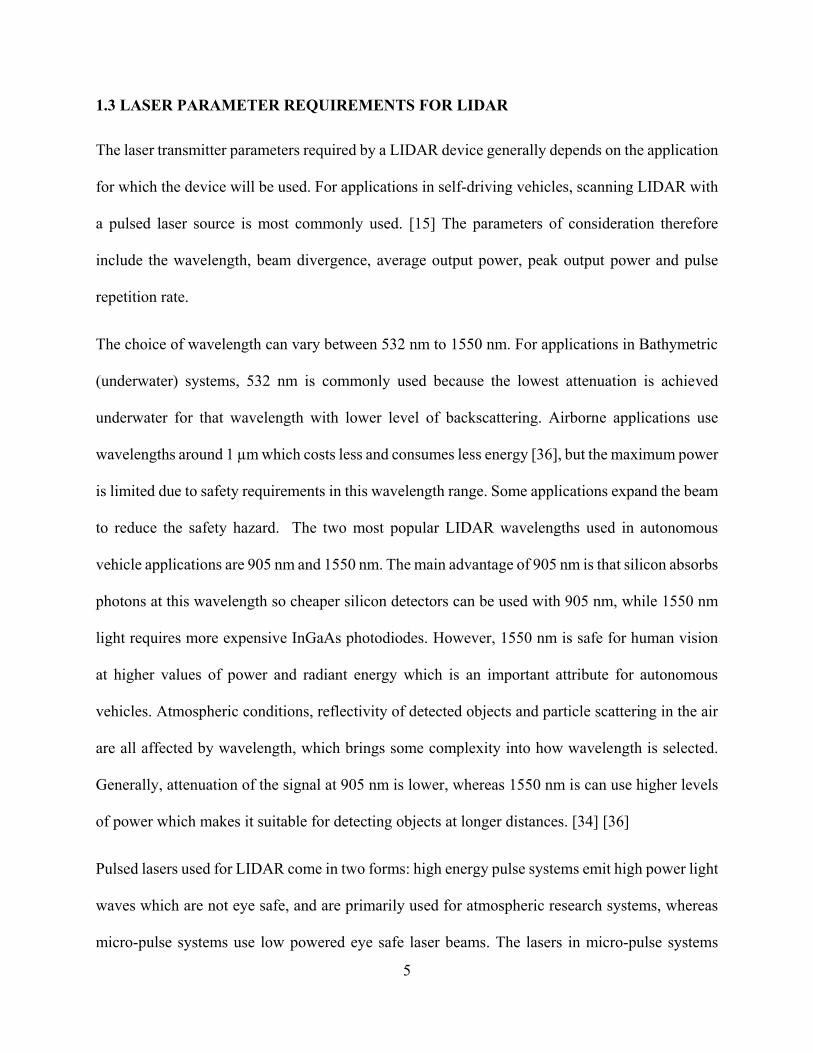
The effect of beam divergence on a LIDAR system can be seen in figure 1.3 below. For scanning
LIDAR systems where each point in a scene in scanned and stored to create a 3-D image, beams
with high divergence can lead to inaccurate detection of objects leading to a loss of finer details in
the detected image. Sources with lower beam divergence leads to more accurate and detailed
images with better resolution. Beam divergence also limits resolution for objects located further
away from the source and ideally a fully collimated beam is required for LIDAR sources, and
Figure 1.3 Effect of beam divergence in LIDAR
7
efforts are being made towards making the beam divergence as small as possible in practical
devices.
1.4 THESIS OUTLINE:
The rest of the thesis is organized as follows:
Chapter 2 introduces the different methods of steering optical beams and discusses some important
work done related to optical beam steering in recent years. The chapter explains how LIDAR is
used in autonomous vehicles, and why non-mechanical beam steering methods are essential in
creating more effective LIDAR devices. Optical phased arrays and MEMS based scanning
systems, which are the most popular technology behind optical beam steering, are discussed in
detail. Current progress in optical phased array and MEMS technology is examined and the
specifications of each work is presented. The chapter also introduces past work done in optical
beam steering using focus tunable lenses, which is the basis of this research.
Chapter 3 discusses the methodology behind the beam steering system of this work. It starts by
introducing the principle behind focus tunable lenses and its features. It also talks about the optical
design software Zemax which was used to simulate the system. Next, it explains how beam
steering is achieved with focus tunable lenses by demonstrating the effect of using one and then
two lenses on a beam. The other elements of the system, their features and purpose is discussed
next. And finally the various steps of the design process are explained, and the results obtained
from each step are displayed. The different design stages are explained, the changes made in the
designs and its effect is also presented. Finally, the size, scan angle and beam divergence from
each stage is compared.
8
Chapter 4 concludes the work and summarizes the results achieved from it, and discusses future
improvements that can be made.
9
2. LITERATURE REVIEW
2.1 LIDAR IN AUTONOMOUS VEHICLES
The idea for autonomous vehicles originated as early as 1939 when the General Motors Futarama
exhibit at New York World’s Fair introduced the idea for radio-controlled self-driving vehicles.
But lack of suitable technology hindered sufficient progress to be made towards developing this
idea. The research behind self-driving vehicles gained attention again in 2004, when the Defense
Advanced Research Projects Agency (DARPA) created it first Grand Challenge, where contestants
were promised $1 million for creating an autonomous vehicle that could drive about 150 miles in
the Mojave Desert. None of the contestants completed the challenge that year, but the same
challenge was completed by 5 contestants in 2005 using improved technology. The technology
used, and feats gained by the vehicles in the race stirred interest among major companies like
Google to start their own self-driving car research division called Waymo in 2009, followed by
other companies like Tesla, General Motors, Toyota, and many more. [22] [15] [24] [25]
Current state of autonomous vehicles is still far from reaching level 5 autonomy, which refers to
cars that can travel completely without the help or presence of a human driver. This requires
artificial intelligence to gather data from sensors that detect roads, obstacles, traffic lights etc. and
process the information to ensure safe operation of the vehicle. Different types of sensors can be
used to detect the vehicle’s surroundings, and each comes with their own merit. [22]
Both long and short range radar is capable of measuring distance and velocity of moving objects,
but falls short in terms of resolution of detected images, and the accuracy due to the longer
wavelength of radio waves. Optical cameras on the other hand can capture high resolution images,
and can even distinguish between the color of objects making it particularly useful in reading
10
traffic lights and signals. They cannot however, capture the specific distance of an object or the
velocity of moving objects, nor are they reliable in the absence of daylight when they can easily
miss a pedestrian walking by. [22]
LIDAR works in similar principle as radar by sending pulses of laser to hit an object and measure
its distance by calculating how long it takes for the laser pulse to travel back. The advantage it has
over radar is the smaller wavelength of light, which makes LIDAR produce higher resolution
images. LIDAR is capable of capturing minor details in scenery more efficiently than even high
resolution radar devices (as depicted in figure 2.1 below), which makes them essential in sensing
systems of autonomous vehicles. [26] [22]
The ultimate solution is to use all these sensors together to achieve maximum efficiency in the
detection of surroundings, so that the benefits of each type of sensor can be utilized.
Figure 2.1 Image detail of LIDAR vs high resolution radar [26]
11
2.2 NEED FOR NON-MECHANICAL BEAM STEERING IN LIDAR
Laser is an essential component of LIDAR systems. Laser beams are fired from the LIDAR and
returns to the device which then calculates the time taken for the round trip. The round trip time
and the known value for the speed of light can therefore give the precise distance of the object
from the LIDAR sensor. This describes one cycle of detection (or one pulse from a pulsed laser
source) which gives the data for one point of the object being detected. With the following cycle,
the point next to the one previously detected can be mapped, and then the next, and so on. Thus,
with a laser source firing thousands of pulses per second, and consequently detecting thousands of
different points of an object, a detailed 3-D image of the object can be modeled from the data
received. But to detect the different points of the object, the light emitted from the laser needs to
be focused on different points on the object. And therefore, the light emitted from the LIDAR
transmitter needs to be physically rotated to scan different spots.
Figure 2.2 Velodyne’s HDL 64-E spinning LIDAR with a 360° horizontal
FOV is extensively used in autonomous vehicles [38]
12
When it comes to autonomous vehicle applications, a LIDAR transmitter needs to scan the entire
360° surroundings of the vehicle to ensure complete safety of the people inside or outside the
vehicle. In current autonomous vehicles, the LIDAR transmitter is perched on top of a mechanical
gimbal, and the entire device is mechanically rotated to map the surroundings. Figure 2.3 below
shows mechanically steered LIDAR devices mounted on top of self-driving car models by Uber
and Google. The need for gimbals and mechanical rotating mechanisms makes these LIDAR
devices bulky, expensive and inefficient. In fact, one of the reasons why self-driving cars are too
expensive for practical use is because a single LIDAR device could cost up to $60,000. [22]
Another consideration for a LIDAR beam scanner is its continuous scanning capability.
Continuous scanning plays a major role, particularly for autonomous vehicle systems, as important
points in a scan may be missed out with LIDAR systems only capable of scanning discrete points.
Figure 2.3 Self-driving vehicles by Uber and Google with spinning LIDAR sensors mounted on top of them.
The LIDAR device spins mechanically to capture a 360° view of the vehicle’s surroundings [39] [43]
13
In fact, according to [10] high speed continuous beam scanning is more important for such
applications than a scanner that can scan in two axes.
2.1.1 OPTICAL PHASED ARRAY
The term phased array refers to the arrangement of individual antennas with controlled phase
relationships such that they emit radio waves which combine in a certain way to control the
direction of the emitted beam. Each antenna in a phased array is equipped with a phase shifter
which is fed with current signals from the transmitter. The current signals determine the phase
relationship of the antennas so that the beams they emit combine either constructively of
destructively resulting in the emitted beam from the phased array to point in the direction of the
greatest constructive interference. This is demonstrated in figure 2.4 below. Phased arrays require
individual antennas, with individual phase shifters for each antenna and other controlling
electronics. Therefore, there can be thousands of individual elements in a phased array, which
makes it impractical for low frequency applications as the device size would be to large. [27]
14
Optical phased array (OPA) refers to an arrangement whose purpose is control the direction of an
optical beam. Unlike the phased arrays discussed above, the electronics involved in optical phased
arrays do not emit the light waves but only control the direction of the light waves produced by a
separate laser device. The beam emitted from the laser is split into channels, and the phase of each
of these channels is controlled by individual phase tuners to steer the beam into the desired
direction. [28]
There have been many different methods used for creating an OPA, some have the drawback of
requiring delays to stabilize the device after each scan which greatly slows down the scanning
process, especially in the case of continuous scanning [10]. Even with extensive research in the
area of optical phased arrays, a major disadvantage in OPA technology is the presence of grating
lobes and side lobes. For emitters in an OPA which are which are spaced evenly and greater than
half a wavelength apart, grating lobes are generated along with the main lobe which limits the
steering angle range. The power emitted between adjacent grating lobes are called side lobes. [29]
Figure 2.4 Optical phased array principle [37]
15
Power generated in these lobes travel in different directions than the main lobe causing losses,
increasing crosstalk and reducing the efficiency of the device. [10]
Yaacobi et al aimed to tackle some of the issues present in OPA technology in [10] which
introduces improvements in wide angle beam scanning using OPA. The optical phased array is
fabricated on a 300 µm CMOS compatible platform using silicon based components which limits
the device to be only usable for wavelengths above 1.25 µm. It employs cascaded phase shifting
architecture with sixteen grating based antennas each 32 µm long, with a 2µm pitch creating a 32
µm × 32 µm array. The device achieved a continuous 1-D scanning angle up to 51° with a
maximum steering speed of 5×10⁶ deg/sec. However, the 32 µm rectangular aperture results in a
considerably large beam divergence of 3.3°. In addition to that there is considerable power loss in
the side lobes which makes the device only 25% efficient.
Poulton et al in [16] suggest an all-in-one LIDAR device with the transmitter, receiver and optical
phased array for beam steering integrated into one chip. Similar to the architecture described
Figure 2.5 Cascaded phase shifting architecture [10]
16
above, this device was fabricated on a silicon photonics platform which is CMOS compatible
which makes the device only compatible for wavelengths above 1.1 µm. The array is composed of
50 antennas each 500 µm long with a 2 µm pitch. The steering angle range achieved in 2-D was
46°×36° with beam divergence of 0.85° which is considerably smaller than [10]. The power
consumption of the device however was high at 1.2 W with high power in the grating lobes along
with the main lobe. The maximum range achieved was also limited to 0.5 m by the aperture size.
In an effort to increase the steering angle range of OPA architecture, Hutchison et al [29] proposed
a new emitter architecture which uses non-uniform emitter spacing and wide angle emitters to
suppress grating lobes which limit the steering angle range in traditional OPA devices. A very
wide angle steering range was achieved which was 80° with low divergence of 0.14°. The tradeoff
here for high steering range was increased side lobe power.
Figure 2.6 Simulation of the OPA from [29] showing beam steering using (a) uniform
emitter spacing, and (b) non uniform emitter spacing. The beam is steered to 10 different
angles in (b) compared to 2 different angles in (a). Also, there is presence of higher side
lobe power in (b). (c) shows a close-up of the main lobe
17
A fully integrated beam steering chip was proposed by Hulme et al in [2]. The device consisted of
164 optical elements to steer an optical beam emitted from a laser which was integrated into the
photonic integrated circuit built on a hybrid silicon platform. The device was composed 2 tunable
lasers, 34 amplifiers, 32 photodiode and 32 phase shifters among other components (figure 2.7
below). The basic principle behind steering the beam in 2-D was wavelength tuning combined
with optical phased array, because using optical phased array for 2-D beam steering required N2
components compared to N components needed for 1-D beam steering. Utilising wavelength
tuning reduced the number of components to N + M where M is the number of components in the
tunable lasers [2]. The steering range achieved using this method was 23° x 3.6° with beam
divergence of 1°.
The table below summarizes the results from each of the optical phased array architectures
described so far. Although high scan angles and low beam divergence can be achieved from these
Figure 2.7 Fully integrated hybrid silicon 2-D beam scanner with 164 optical
elements [2]
18
OPA devices, the presence of secondary power in the side and grating lobes reduces their
efficiency and accuracy of the scan.
2.1.2 MICRO-ELECTROMECHANICAL SYSTEMS (MEMS)
Micro-electromechanical systems (or MEMS for short) has recently gained much popularity in
beam steering applications. Many newly found companies specializing in LIDAR like Infineon
[42] are now focusing on using MEMS technology in their LIDAR devices. A MEMS device
consists of an IC chip with several microscopic components are integrated to make one complete
mechanical system in microscopic form. It consists of micro-sensors, microelectronics and
micromechanical systems. These devices work together to detect input signals and process the
input to perform the corresponding mechanical output. MEMS components are all manufactured
at the microscopic level, even components like levers, gears and motors are created in microscopic
sizes. [31]
Largest scan angle achieved
in any direction
Beam
divergence
[10] 51° 3.3°
[16] 46° 0.85°
[29] 80° 0.14°
[2] 23° 1°
Table 2.1 Comparison of different OPA technologies in terms of scan angle and beam divergence
19
MEMS based scanning mirrors are commonly used for LIDAR applications. These devices are
composed of a tiny scanning mirror which is controlled by microelectronic and micro-mechanical
elements which controls its direction of movement. An array of such MEMS based scanning mirror
is what makes up a Digital Micro-mirror device, which is the main mechanism behind the beam
steering system in [3] proposed by Smith et al. Each MEMS mirror in a DMD acts as a pixel which
is all controlled by microelectronics that come together in the chip. The DMD is used in [3] to
create a programmable blazed grating by controlling the individual mirrors using an Arduino
controller. Discrete beam steering was demonstrated for five different angles corresponding to five
different diffractions orders of the grating.
A collimated 8ns pulsed laser source was used with a wavelength of 905 nm. The beam scan at the
five diffractions orders can be seen in figure 2.10 below.
Figure 2.8 A MEMS scanning mirror [41]
20
It can be seen from the scan that there is presence of crosstalk between all the diffraction orders
and the 0th diffraction order. This crosstalk originates from the reflection at the mirror which causes
detection from the 0th order when the object comes close to the device. The device achieved scan
angle of 48° and a measurement accuracy of less that 1cm.
Figure 2.9 Setup of the beam scanning system using DMD [3]
Figure 2.10 Beam scan using DMD showing the beam at 5 discrete beam scanning points. The
presence of crosstalk between the other orders and the 0th order can be seen in the scans. [3]
21
Hofmann et al. [45] introduced an automotive LIDAR device utilizing a MEMS scanning mirror
coupled with an omnidirectional lens, which is capable of scanning in all directions. The device
setup shown in figure 2.11 below consists of a 2-D MEMS scanning mirror capable of tilting by
15° on both axes. A large mirror aperture of 7mm diameter is selected to allow the device to
measure larger distances. To facilitate circular scanning in all directions, a special tripod MEMS
mirror was designed and fabricated.
Figure 2.11 2-D MEMS scanning mirror coupled with omnidirectional lens [45]
2.1.3 BEAM STEERING WITH FOCUS TUNABLE LENSES
Wide-angle beam steering using focus tunable lenses was introduced by Zohrabi et al in [5]. Focus
tunable lenses are composed of optical fluid enclosed in an elastic container which can change
shape when pressure is applied to it in the form of electrical signals. The change in shape
corresponds to change in the focal length of the lens. More details about focus tunable lenses are
presented in the next chapter.
22
Zohrabi et al used two tunable lenses with other optical components to create a wide angle beam
steering mechanism which is based on controlling the focal length of the two tunable lenses. Beam
steering in 1-D was achieved with a total scan angle of about 78°.
The major drawback here however is the large size caused by the length of the optical path. The
device was modified to scan in 2-D by adding a third tunable lens, and the scan range was increased
to ±75° by employing a fisheye lens to widen the scan. This however further increases the device
size. The figure 2.13 below shows the position of the third tunable lens for 2-D scanning with the
fisheye lens to widen the scan angle further. It can be seen that the fisheye lens contributes to
increasing the size of the device further. Figure 2.14 shows the scan results from both setups. The
first figure 2.14 (a) shows a 1-D scan of 39° on either side from the center resulting in a total scan
angle range of 78° whereas (b) shows the beam travelling 75° on either side resulting in a 150°
scan.
Figure 2.12 Beam steering using focus tunable lenses [5]
23
Figure 2.13 Increasing scan angle using fisheye lens [5]
Figure 2.14 Experimental setup of the device (a) without and (b) with the fisheye lens
showing scans of ±39° and ±75° respectively [5]
24
3. BEAM STEERING USING FOCUS TUNABLE LENSES
3.1 FOCUS TUNABLE LENSES
The key mechanism used in controlling the direction of the laser beam in this work is focus tunable
lenses developed by Optotune. The basic structure of the focus tunable lens comprises of optical
fluid (with low dispersion, and refractive index of 1.30) enclosed in an elastic container with sealed
ends. The tunable lens is driven by electric current which controls the pressure exerted on the
elastic container housing the optical fluid thereby changing the shape of the container. This change
in shape corresponds to the change in the radius of curvature of the lens, and therefore the focal
length is controlled through the input current. The optical power of the lens (which is the inverse
of the focal length), varies linearly with the current. [11]
The range of values between which the focal length of the lens can be tuned depends on the
membrane thickness of the container enclosing the optical fluid. Larger ranges of focal length can
be achieved from lenses made of thinner membranes than those with thicker ones. Most lenses
Figure 3.1 Optotune’s EL-10-30-TC focus tunable lens [13]
25
have optical powers which can only be tuned between positive values i.e. they can only act as
convex lenses. Other lens models have a concave offset lens to provide negative optical power
values. Some models also have the capability to use the pressure exerted on the lens membrane to
create a concave lens shape. [11]
Another important parameter of consideration when using focus tunable lenses is the response
time. Due to the inertia of the optical fluid, there is a slight delay in the application of current to
the change in the focal length of the lens. The response time is usually a few milliseconds and can
vary between 2-12 milliseconds depending on the model of the lens. [11]
3.1.1 ELECTRICALLY TUNABLE LENS EL-10-30
The EL-10-30 is the most versatile plano-convex lens model made by Optotune. Although the
optical power can only take positive values, it has one of the largest range of values for tuning the
focal length. And it is also capable of reaching the greatest optical power (up to 20 diopters)
compared to all the other lens models. The EL-10-30 comes in two different types of housing, the
EL-10-30 TC which is a compact version, and the EL 10-30-C. The two models have similar
specifications except for some differences in dimension and focal tuning range which is
summarized in Table 3.1 below. [12]
Lens model Dimension (mm)
Focal length tuning
range
Optical power
range (diopter)
EL 10-30 TC 30 x 10.7 +50 to +120 +8.3 to 20
EL 10-30 C 30 x 20 +100 to +200 +5 to +10
Table 3.1 Comparison of two different tunable lens models
26
The graph below shows the relationship between optical power and current for the different EL-
10-30 lens models. The two variations of the C model differ only in that the second model comes
with an option for an offset lens which allows for the lens to reach negative optical powers. The
optical power can then be tuned from -1.5 to 3.5 diopters, and so the range remains the same. [12]
Nominal values of input current for the lens are between 0-250 mA, although currents up to 400
mA can also be applied. [12] It can also be seen from the slope of the different lines, that the EL-
10-30 TC has a greater range of optical power values for the same input current.
For this work the EL 10-30 TC model was chosen because of two reasons. First, the EL 10-30-TC
is smaller in size compared to the EL 10-30 C model, which is important for making our design as
compact as possible. Secondly, the TC model also has a thinner membrane which is why it is
capable of achieving higher optical power and has a greater range of optical power tuning which
Figure 3.2 Optical power vs current for the EL-10-30 series [12]
27
is also essential for a more compact device, as it can produce a larger scan within a shorter optical
path length. The EL 10-30 model also has the smallest response time of less than 2.5 milliseconds
among all the tunable lens models. [12]
3.2 ZEMAX DESIGN SOFTWARE
Zemax OpticStudio software was used for simulating the beam scanning system. OpticStudio is a
powerful tool for designing all kinds of optical systems and analyzing them using its ray tracing
feature. It has two modes of operation: sequential and non-sequential mode.
3.2.1 SEQUENTIAL MODE AND NON-SEQUENTIAL MODE
Sequential and non-sequential design modes differ mainly in the way the light rays propagate
through the system. In sequential design, rays follow a predetermined path hitting each object in
the exact sequence as they are defined in the Lens Data Editor. Analysis of stray light or light
scattering is impossible in the sequential mode as the light rays (which are predefined by the editor)
cannot follow random paths in a system. For such analyses, the non-sequential mode is useful. In
the non-sequential mode, rays defined in the design do not follow any predefined sequence. The
path followed by the ray and the sequence of objects the ray hits completely depends on the
direction of the ray and the position of the object. [17]
The two modes also differ in the way objects are defined. In the sequential mode, each object is
defined by its individual surfaces. For example, to create a plano-convex lens, two individual
surfaces must be created: the lens front which will define the radius of curvature of the lens, and a
flat lens back which will have a radius of curvature of zero. On the other hand, in the non-sequential
28
mode, objects are defined as a whole and not as individual surfaces. Therefore, the same plano-
convex lens can be defined as one object. [17]
The non-sequential mode is a more versatile tool as any kind of 3-D surface can be modelled in it.
Non-sequential mode was utilized in this work, as the design involved the use of many objects that
can only be modelled as non-sequential objects in Zemax like prisms and a diffuser. [17]
Figure 3.3 Modelling a simple lens using Sequential and Non-Sequential mode in Zemax OpticStudio.
The lens is modeled as two separate surfaces in the Sequential mode whereas it is modeled as a single
object in the Non-Sequential mode
29
3.3 SYSTEM ELEMENTS AND DESIGN
3.3.1 MODELLING TUNABLE LENSES IN ZEMAX
The Zemax model for the EL-10-30 TC and other tunable lens models can be found from the
Optotune website [12]. The Zemax model for the EL-10-30 TC is shown in figure 3.4 below. The
focal length of the lens can be tuned between +50 mm to +120 mm, although only the radius of
curvature can be modified in Zemax. Using Zemax simulation and measurement, the radius of
curvature of the lens was found to be 14mm when the focal length was set to 50 mm. In the same
way, the radius of curvature corresponding to a focal length of 120 mm was found to be 38mm.
Therefore, the radius of curvature of the lens is tunable between 14mm to 38mm.
Figure 3.4 Zemax model for EL 10-30 TC modeled in Sequential mode
of Zemax. The complete model shows the tunable lens along with the
lens housing and cover glass
Lens housing
Cover glass
Light source
Tunable lens
30
Figure 3.5 below demonstrates the focal point of the lens when the radius of curvature is set to 14
mm and 38 mm respectively.
3.3.1.1 EFFECT OF CHANGING CURVATURE OF ONE LENS ON THE BEAM
To demonstrate the effect that changing the focal length on the optical beam, the beam must be
decentered along the y axis with respect to the lens. In figure 3.6 below, the beam is decentered by
2 mm on the y axis, and the focal length is set to 20mm by setting the radius of curvature of the
lens to 6mm (this is beyond the range of the actual lens, but it is used for the sole purpose of
demonstration). With the object at the same distance from the lens, the radius is now changed to
5mm and then 7mm. It can be seen from the figures, that the beam changes position on the object,
but it becomes defocused on the object. Therefore, to move the beam and still keep it focused at
the same distance from the lens, two tunable lenses must be used, as discussed in the next section.
[5]
Figure 3.5 Tunable lens focal length set to 50 mm and 120 mm
31
3.3.1.2 STEERING A BEAM WITH TWO TUNABLE LENSES
To steer the beam and also keep it in focus on the image plane, two lenses must be used. In figure
3.7 below, the two lenses are placed 15mm from one another, and the second lens is decentered
4.3mm along the y axis with respect to the first lens. The radius of curvature of both lenses is set
to 25mm and the beam focuses 45 mm away.
In the second image the radius of curvature of the two lenses are now changed to 19 and 37 mm
respectively. The beam focus displaces by 0.7 mm on the y axis, indicating beam steering on the
y-axis. However, the beam still remains focused at the same distance of 45 mm.
Figure 3.6 Effect of adjusting the radius of curvature of the lens on the beam. The
radius of curvature is set to 5, 6 and 7 mm.
32
3.3.2 RELAY LENS
An achromatic doublet lens is placed after the second tunable lens and it acts as a relay lens to
focus the beam from the tunable lenses. The architecture of an achromatic doublet lens consists of
two lenses attached together one with a positive focal length and the other with a negative focal
length. The two lenses are also made with materials of different indices of refraction, and different
dispersion characteristics. Achromatic doublet lenses are commonly used to correct the effects of
chromatic and spherical aberrations. [18] The lens model used here is equivalent to the model
AC080-010-C-ML from Thorlabs, with a focal length of 10mm [23]. The lens works to focus the
incoming laser beam from the tunable lenses onto the diffuser [5]. The diagram below shows the
achromatic doublet lens modeled in Zemax.
Figure 3.7 Beam steering using two tunable lenses
33
3.3.3 FOLDED OPTICS
The optical path length between the achromatic doublet lens and the diffuser in [5] plays an
important role in determining the scanning angle range of the design. Because of the high focal
length of the tunable lenses, to achieve significant steering of the optical beam, a very high path
length is required between the relay lens and the diffuser. And this high optical path length makes
the design very large, making it impractical.
To tackle this issue, the principle of folded optics was used. The idea here is to fold the optical
path thereby reducing its longitudinal size. A similar idea is used in binoculars that use Porro
prism. Two prisms are set with their bases facing each other with one prism rotated along one axis
with respect to the other. This reduces the size of the binoculars by reducing the optical path length.
[20]
The setup used in this work is shown in figure 3.9 below, with two 90° prisms with their base
facing each other. When the light enters the through the base of the first prism, total internal
Figure 3.8 Model of the achromatic doublet lens on Zemax
34
reflection occurs when it hits the other two faces of the prism. The light then exits the first prism
in the opposite direction and enters the second prism through its base and repeats the process.
For the above process to take place, the prism base length l, the distance between the prisms g, and
the displacement along the base d must be selected to that the light rays enter both the prisms and
total internal reflection takes place in both prisms. In general, for the arrangement shown in figure
3.9 above, incoming beam will go through 2N total internal reflections, and N is determined by
the formula:
𝑁 = 𝑟𝑜𝑢𝑛𝑑 (𝑙
𝑑) (3.1)
Where round refers to rounding the result to the nearest integer. If g is the length of the gap between
the prisms, and n is the refractive index of the prism material, the total optical path length that the
beam will now travel is given by the formula [19]:
l
d
g
Figure 3.9 Prism layout for folding the optical path
35
∆ = 𝑛𝑁𝑙 + 𝑁𝑔 (3.2)
The dimensions used in this work are shown in figure 3.10 below. The prisms used had a base
length of 28 mm and were placed 40 mm apart, and displaced by 14 mm. The material used was
N-BK7 glass with a refractive index of 1.5 at 1550 nm wavelength. Using equation 3.1 above, with
these values gives us N = 2, and as seen from the figure below, the beam experiences total internal
reflection 4 times.
Using these values in equation 3.2 above, we get the total optical path length as
∆ = 164 𝑚𝑚
Indicating that the beam travels a total of 164 mm between the two prisms.
28 mm
14 mm
40 mm
Figure 3.10 Dimensions used for prism layout
36
3.3.4 OPTICAL DIFFUSER
Optical diffusers are used to scatter or “soften” the light passing through them. They are made of
different materials, and the most common diffusers are made with N-BK7 ground glass material.
[21] The light is focused onto the diffuser from the relay lens and it acts as a point source of light
whose position depends on the focal length of the tunable lenses. The diffuser increases the
numerical aperture of the beam so that the beam can be steered through a larger angle.
The diffuser is modelled in Zemax as a cylindrical volume object. The back face of the cylindrical
object has a BSDF scatter model with a scatter angle of 15°. This emulates the working principle
of a ground glass N-BK7 diffuser with a diffusion cone angle of 15°. The diagram below shows
the effect of the diffuser on the incoming laser beam.
Figure 3.11 Diffuser modeled in Zemax OpticStudio with a diffusion cone angle of 15°
37
3.3.5 OBJECTIVE LENSES
The final step in the beam steering process is further increasing the scan and focusing the beam
using two objective lenses. The objective lenses also collimate the diverging beam coming from
the diffuser which acts as point source. A plano-convex and a double convex lens is used one after
the other to focus the beam emitted from the diffuser onto the detector. The lenses used in the final
design are equivalent to models LA 1951.1 and LB 1761.1 by Thorlabs both with focal lengths of
25 mm. [23] Objective lenses with a focal length of 50 mm were used in [5], but a lower focal
length was used in this work as it leads to a higher range of scanning angle. The lower focal length
also works to reduce the divergence of the beam and create a more collimated beam as will be seen
later.
Figure 3.12 Plano-convex and double convex objective lens models on Zemax with focal lengths of
25mm
38
3.4 SIMULATION AND RESULTS
This section discusses the simulation results for the different versions of the design. Three different
simulations were made which will be discussed. The first one replicates the design and result of
that obtained by Zohrabi et al in [5]. Since the design is far too large in size because of the optical
path length between the relay lens and the diffuser, the effect of reducing the optical path length
is also discussed. Finally, folded optics is incorporated in the design along with objective lenses
with a smaller focal length. Folded optics reduced the longitudinal size of the device, whereas the
change in focal length of the objective lenses increased the scan angle and resulted in a more
collimated beam.
3.4.1 CASE 1
In the first simulation, the tunable lenses were placed 41 mm away from one another and the relay
lens was placed 22 mm away from the second tunable lens. The diffuser was placed 280 mm from
the relay lens, and objective lenses 50 mm in focal length followed the diffuser placed 12mm and
6mm apart. The rays start from the source object to the left of the first tunable lens and are finally
cast onto a detector that is placed 85 mm from the last lens surface. Three beams are displayed in
the figures below, slightly displaced along the lens on the y-axis. This replicates the effect of
changing the radius of curvature of the tunable lenses while keeping the source in the same
position. The detector here acts as the object which will be scanned by the LIDAR system. The
detector comes with ray tracing capabilities, with which we can detect the position of the ray on it
for a specific focal length of the tunable lenses. The ray trace shown in figure 3.15 shows the
position of the ray on the detector when the radius of curvature of the lens is adjusted to different
values.
39
From the 3-D model shown above, it can be seen that there is a big gap between the relay lens and
the optical diffuser. This gap is necessary to provide sufficient path for the light rays to travel and
fall on the right point on the diffuseraf to ensure wide angle scanning. The entire device setup is
385 mm long which is a drawback as the device too large for practical use in LIDAR systems.
Figure 3.13 3-D cross section model for Case 1
40
The scan angle is calculated from the ray trace results shown below. The diagrams show the results
obtained from the ray tracing tool in Zemax. Figure 3.15 (a) shows the physical position of the
beam falling on the detector when the radius of curvature of the tunable lenses are tuned between
the values of 14 mm and 38 mm. It can be seen that the beam changes position along the y-axis
demonstrating 1-D beam steering along the y-axis. The same result is represented in graphical
form with the incoherent irradiance, which is a measure of the intensity of the beam, plotted against
its position on the y-axis.
Figure 3.14 3-D shaded model for Case 1
41
Figure 3.15 Diagram showing the results from the ray tracing tool in Zemax. (a) shows the
physical position of the beam moving along the y-axis at different values of focal length of
the lenses. The incoherent irradiance of the beam is the measure of the intensity of the
beam. (b) shows the same result in graphical form making it easier to locate the beam on
the y-axis
42
Figure 3.15 (b) shows the location of the beam’s peak more accurately. It can also be observed
that the beam instensity falls as it moves further away from the center where it is at its peak. This
drop in intensity also coincides with the fact that the beam diverges more as it is steered further
from the the center. This increase in beam size results in an overlap of the rays traced at y-
coordinate positions +45 and +66 on the detector.
The beam from the device falls onto the detector which is placed 85mm away, and moves up to
66mm away from its center position on the y-axis. This is represented in figure 3.16 below.
Using rules of trigonometry, as shown below, α is found to be 37.8° meaning the beam moves
37.8° on both sides away from the center. Therefore the total scan angle is found to be 76°.
α = tan−1 66
85
a
85 mm
66mm
Figure 3.16 Calculating beam scan angle. The base of the triangle represents the detector
on which the beam travels along the y-axis.
43
α = 37.8°
Total scan angle = 2α = 76°
Although this design is capable of scanning over a wide angle, the major drawback is that the long
optical path makes the device very big. The effect of reducing the optical path will result in a much
smaller scan angle as will be seen in the next section.
3.4.2 CASE 2: REDUCING THE OPTICAL PATH LENGTH
In an attempt to reduce the longitudinal size of the device, the optical path length between the relay
lens and diffuser was reduced from 280mm to 55mm. The tunable lenses were placed 10mm apart
and the relay lens was placed 12 mm from the second tunable lens. The resulting ray trace is shown
below, with the detector placed at the same distance from the last surface (85 mm). It can be seen
that there is a significant reduction in the scan angle once the optical paths are reduced.
From the ray trace results shown in figure 3.19, the beam moves 12 mm on the y axis in both
directions away from its center position. Using the same principle as in section 3.4.1 above, the
scan angle is calculated as 8° in both directions, resulting in a total scan angle of 16°.
In this version of the design, the size of the device is reduced to only 114 mm, but the
corresponding steering range is too small. The next design attempts to tackle this by employing
folded optics to tackle the issue of size and at the same time increase the scan angle to a higher
value.
44
Figure 3.187 3-D cross section model for Case 2
Figure 3.178 Shaded model for Case 2
45
Figure 3.19 Ray traces obtained from the design after reducing the optical path length
shows its effect. It can be seen that the beam moves between a much smaller range than
before
46
3.4.3 CASE 3: INTEGRATING FOLDED OPTICS INTO THE DESIGN
In an effort to reduce the length of the device, and at the same time increase the scan angle, two
design changes were made:
• Prisms were used in the optical path between the relay lens and the diffuser to fold the path
of light, thereby reducing its length
• Objective lenses with lower focal lengths value were used after the diffuser to increase the
scan angle.
In this final design, the tunable lenses are placed 10 mm apart and the relay lens is placed 15 mm
from the second tunable lens. The 280 mm optical path between the relay lens and the diffuser in
the first design, is replaced by the prism arrangement shown in figure 3.10 earlier. The diffuser is
placed 60 mm after the base of the second prism with objective lenses of 25 mm focal length
following the diffuser.
Figure 3.22 shows the results of the ray trace. It can be seen that the beam now travels between
farther along the y-axis. From figure 3.22 (b) the beam is measured to steer 42 mm away from the
center on both sides. Using the same calculations as 3.4.1 above, this corresponds to a steering of
26° on both sides, meaning a total scan angle of 52°. This is a significant increase in the scan angle
from the last design. At the same time, it can be seen from the figure above that the entire length
of the device is about only 119 mm which is also a major reduction in size from the first model.
Furthermore, it is visible from the two ray trace diagrams and the 3-D model that the higher power
of the objective lenses are much more efficient in producing a low divergence beam with higher
values of incoherent irradiance.
47
Figure 3.20 3-D cross section model of final design using prisms and objective lenses with a smaller focal
length
Figure 3.21 3-D shaded model for Case 3
48
Figure 3.202 Ray trace results for Case 3
49
3.4.4 CASE 4
Case 4 was simulated by adding another prism to the design of Case 3 to further increase the path
length and subsequently, the scan angle. The figure below shows the design layout.
The results of the ray trace are shown in figure 3.24 below. Even though addition of a third prism
leads to an increase in path length, the corresponding scan angle is only increased to 60°. This is
due to the fact that not all values of focal length of the tunable lenses could be used in this design,
as using higher values of focal length caused the rays to rays to take unwanted paths and reflect
among the prisms instead of reaching the optical diffuser. Thus, a lower range of focal length
values used lead to a lower range of scan angle than expected.
60 mm
85 mm
Figure 3.213 3D layout for Case 4
50
Figure 3.224 Ray trace results for Case 4
51
3.5 COMPARISON OF SIZE, SCAN ANGLE AND BEAM DIVERGENCE
3.5.1 COMPARING THE PHYSICAL LENGTH VS OPTICAL PATH LENGTH
Figure 3.25 below compares the distance between the relay lens and the diffuser of the first and
the final design. In the first design, the physical length between them is 280 mm which is the same
length as the optical path. In the final design, the physical distance between the relay lens and the
diffuser is only 48 mm. The total optical path length, however, is the sum of the path length
travelled between the two prisms, as calculated in section 3.3.3 and the distance between the
second prism and the diffuser. Therefore, the total distance the rays travel between the relay lens
and the diffuser is:
∆ = 164 + 60 = 224 𝑚𝑚
Figure 3.235 Comparing the optical path length and the physical length between the relay lens and the
diffuser in Case 1 and Case 3
280 mm
48 mm
60 mm
52
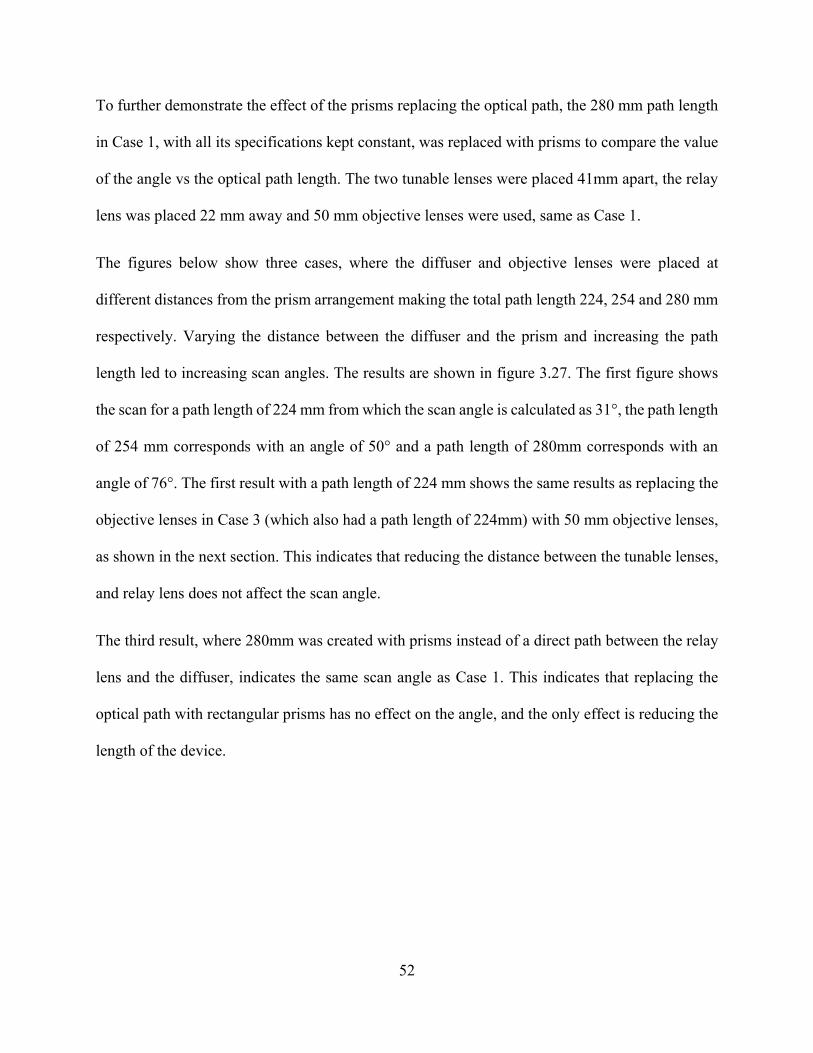
To further demonstrate the effect of the prisms replacing the optical path, the 280 mm path length
in Case 1, with all its specifications kept constant, was replaced with prisms to compare the value
of the angle vs the optical path length. The two tunable lenses were placed 41mm apart, the relay
lens was placed 22 mm away and 50 mm objective lenses were used, same as Case 1.
The figures below show three cases, where the diffuser and objective lenses were placed at
different distances from the prism arrangement making the total path length 224, 254 and 280 mm
respectively. Varying the distance between the diffuser and the prism and increasing the path
length led to increasing scan angles. The results are shown in figure 3.27. The first figure shows
the scan for a path length of 224 mm from which the scan angle is calculated as 31°, the path length
of 254 mm corresponds with an angle of 50° and a path length of 280mm corresponds with an
angle of 76°. The first result with a path length of 224 mm shows the same results as replacing the
objective lenses in Case 3 (which also had a path length of 224mm) with 50 mm objective lenses,
as shown in the next section. This indicates that reducing the distance between the tunable lenses,
and relay lens does not affect the scan angle.
The third result, where 280mm was created with prisms instead of a direct path between the relay
lens and the diffuser, indicates the same scan angle as Case 1. This indicates that replacing the
optical path with rectangular prisms has no effect on the angle, and the only effect is reducing the
length of the device.
53
41mm 28mm 22mm
60mm
85mm
90 mm
116mm
Figure 3.246 Demonstration of the effect of adding prisms on the optical path length and
the scan angle
54
Figure 3.257 Results from Figure 3.26 above
55
3.5.2 COMPARING BEAM DIVERGENCE USING 50 MM AND 25 MM OBJECTIVE
LENSES
Figure 3.28 below demonstrates the effect of using 50 mm focal length objective lenses vs 25mm
objective lenses. The first set of ray trace shows the result obtained from using 50 mm objective
lenses on the design in case 3, and the second set shows the result of using 25 mm lenses on the
same design. Not only is the scan wider for the second case and reaching farther points along y-
axis, but the beam size is also visibly smaller.
Figure 3.268 Two sets of ray traces (a) using 50 mm objective lenses and (b) using 25 mm
objective lenses
(a) (b)
56
The RMS spot size of the beam in the two cases is calculated using Zemax. For the first case using
50 mm objective lenses, the RMS spot size when the detector is placed 85 mm from the design is
found to be 6.84 mm. And when the detector is moved to 2m away, the RMS spot size increases
to 43 mm due to divergence.
In contrast, when using 25mm objective lenses, the RMS spot radius is 1.82 mm when the detector
is placed 85 mm from the design and expands to 15 mm when the detector is placed 2 m away.
The RMS beam radius vs the distance of the detector from the device is plotted in figure 3.29
below to demonstrate the beam divergence for the two focal lengths. The red line indicates the
values gotten from using a 50 mm lens and the blue line indicated values achieved from using a
25 mm lens.
Figure 3.279 Beam RMS spot radius vs distance from the device
0
5
10
15
20
25
30
35
40
45
50
0 500 1000 1500 2000 2500
be
am r
adiu
s (m
m)
distance (mm)
25mm lens 50mm lens
57
It can be seen from the greater slope of the red line that the beam increases in size much more
rapidly. The blue line has a smaller slope indicating a more collimated beam which is more suitable
for LIDAR applications.
The beam divergence can be calculated for the two models using the beam radius at two different
points away from the origin and the distance between them. Let R1 and R2 be the radii of the beam
at two different positions, and L be the distance between them. Then the beam divergence θ is then
given by:
𝜃 = 2 tan−1 (𝑅2 − 𝑅1
2𝐿 )
Using this formula, the beam divergence for case 3 was found to be 0.45° whereas for case 1 and
case 2 it is 1.73°.
Table 3.2 below summarizes the result from the three designs. In terms of the longitudinal size of
the device, there is a significant reduction in the latter two designs from the original one. The
change is length between the latter two designs is not very significant, as the third design is only
5mm longer than the second one. On the other hand, the total length of the original device is
385mm while the total length of the final device is 119 mm. This corresponds to a 69% reduction
in the length of the device.
Regarding the scan angle, the original device had a higher scan range of 76°. When the optical
path length was reduced in the second model, this scan range dropped to only 16°. Meanwhile the
use of prisms to fold the path of light led to an increase in the scan angle to 52°.
58
Case 1 2 3 4
Total length (mm) 385 114 119 125
Total scan angle 76° 16° 52° 60°
Beam divergence 1.73° 1.73° 0.45° 0.45°
Table 3.2 Summary of results
When comparing the reduction in length vs the scan angle between the first and the last model, the
length is reduced by 69% in the last model. The beam divergence is also reduced by 74%.
3.5.3 EFFECT OF REFLECTION ON THE TOTAL TRANSMITTED POWER
The effects of reflection in the optical components used will affect the efficiency of the system.
The table below lists the percentage transmission of each optical component at 905 nm wavelength,
assuming all components are coated with anti-reflection coating. [12][50][51][52][53][54]
Optical component Transmission at 905 nm with
AR coating (%)
Tunable lens 94.6
Achromatic doublet lens 99.8
90° prism 99.6
Optical diffuser 80
Plano convex lens 99.5
Bi convex lens 99.5
Table 3.3 Percentage transmission of each component at 905 nm wavelength of light
59
Thus, for Case 3 which uses each of these components, 70% of the power transmitted from the
laser will be transmitted through the device. Whereas 69.7% of the power will be transmitted for
Case 4 which uses an additional prism.
60
4. CONCLUSION
4.1 THESIS CONCLUSION
Even though the technology behind LIDAR has been around for many years now, recently there
has been a great deal of research on the topic. Improvements are made on all components of the
device making it suitable for different applications. One of the reasons LIDAR has gained so much
focus recently is its importance in detection systems for autonomous vehicles. Autonomous
vehicles have seen significant improvements recently with major companies around the world all
working towards making them accessible and safe to use for everyone. But even with all the
developments in this area, autonomous vehicles are still far from being efficient enough for
everyday use, cheap enough to be ubiquitous, or safe enough to be driven without a human
controller present. There is still room for lots of improvements to be made in terms of obstacle
detection, like improvements in accuracy of distance measurement, image resolution, detection
speed, or response speed. Improvements are also essential in making the vehicle itself and the
components of the vehicle more efficient and cost-effective so that autonomous vehicles can be
made available to everyone. And for this reason, LIDAR devices need to be cheaper and more
efficient that can capture surrounding images at high resolution.
The mechanical gear used in LIDAR to steer laser beams are the main reason behind their high
cost, and consequently the high cost of self-driving cars. It also makes the LIDAR device bulky
and heavy. The aim of this thesis was to create a non-mechanical system for steering laser beams
which can be used specifically in applications for LIDAR devices in self-driving cars. The system
made use of focus tunable lenses, which uses electrical current to exert pressure on a container of
optical fluid, thereby changing the focal length of the lens. This change in focal length resulted in
61
shifting the position of the beam when two lenses are used one after the other. Other optical
components, like achromatic doublet lens, optical diffuser, and objective lenses were used after
the tunable lenses to focus the beam and increase the angle of the scan. Finally, 90° prisms were
used to fold the optical path to make the device more compact.
Three different design stages were carried out with the goal of improving the scan angle, reducing
the longitudinal size, and reducing the beam divergence.
1. In the first design, the two tunable lenses were placed 41mm apart with the relay lens
positioned 22 mm from the second tunable lens to focus the beam onto an optical diffuser
280 mm away. The diffuser was followed by a plano-convex and a bi-convex objective
lens of 50mm focal length. The entire device was about 385mm long and the total scan
angle was 76°. The beam divergence was calculated to be 1.73°.
2. The second design aimed at finding the effect of reducing the length between the relay lens
and the diffuser. Therefore, the length between the relay lens and the diffuser was reduced
from 280 mm to 55mm. The distance between the two tunable lenses was also reduced to
10 mm followed by the relay lens 12 mm away. The total length of the device was reduced
to just 114 mm, but consequently the total scan angle was also reduced to only 16°. The
beam divergence was the same as before at 1.73°.
3. In the third design, instead of removing the optical path between the relay lens and the
diffuser all together, it was replaced with prisms so the light would reflect along the walls
of the prism, and travel in a folded path and therefore reduce the longitudinal size of the
device. Two prisms were used, and the light rays underwent total internal reflection a total
of four times and were then focused onto the diffuser. The arrangement of the prisms made
the total path travelled by the light to be 164 mm, and with the diffuser placed 60 mm away
62
from the last prism, the total optical path length was 224 mm. This is still lower than the
path length in case 1 where the path length was 280 mm but increasing it any more would
result in a larger setup where our goal is to make the device as compact as possible. The
device size was reduced to 119 mm, and there was a reduction in scan angle which in this
case is 52°. But this angle is still high enough for practical applications.
Another change made in this design was that the focal length of the objective lenses used
after the diffuser were reduced from 50mm to 25mm. This not only increased the scan
angle compared to the second design, but it also resulted in an output beam with
significantly lower divergence angle of only 0.45°.
4. An additional prism was added in the fourth case in an effort to further increase the optical
path length and the angle. Even though the angle increased to 60°, this increase does not
correspond fully with the increase in the optical path. This is because the full range of focal
lengths could not be used in this design, as increasing it beyond a certain value caused the
rays to take unwanted paths and not reach the diffuser.
Comparing the final design of the system with the first one, we can see that there is a 69% reduction
in size with a significant 74% reduction in the beam divergence. Losses due to reflection in the
components was also considered, indicating a 70% efficiency and 905nm.
4.2 FUTURE WORK
Future work related to this thesis can look at a number of factors for improvement including:
1. The scan angle may be further increased by adding more prisms to increase the optical path
of the light.
2. Improvements can be made in increasing the speed of steering the light beam.
63
REFERENCES
[1] C. V. P. and M. R. Watts, “MIT and DARPA Pack LIDAR Sensor onto Single Chip,” IEEE
Spectrum: Technology, Engineering, and Science News, 04-Aug-2016. [Online].
Available: https://spectrum.ieee.org/tech-talk/semiconductors/optoelectronics/mit-LIDAR -
on-a-chip. [Accessed: 07-Jun-2018].
[2] J. C. Hulme et al., “Fully integrated hybrid silicon two-dimensional beam scanner,” Opt.
Express, OE, vol. 23, no. 5, pp. 5861–5874, Mar. 2015.
[3] B. Smith, B. Hellman, A. Gin, A. Espinoza, and Y. Takashima, “Single chip LIDAR with
discrete beam steering by digital micromirror device,” Opt. Express, OE, vol. 25, no. 13, pp.
14732–14745, Jun. 2017.
[4] C. T. DeRose et al., “Electronically controlled optical beam-steering by an active phased
array of metallic nanoantennas,” Opt. Express, OE, vol. 21, no. 4, pp. 5198–5208, Feb.
2013.
[5] M. Zohrabi, R. H. Cormack, and J. T. Gopinath, “Wide-angle nonmechanical beam steering
using liquid lenses,” Opt. Express, OE, vol. 24, no. 21, pp. 23798–23809, Oct. 2016.
[6] J. Kim, M. N. Miskiewicz, S. Serati, and M. J. Escuti, “Nonmechanical Laser Beam
Steering Based on Polymer Polarization Gratings: Design Optimization and
Demonstration,” Journal of Lightwave Technology, vol. 33, no. 10, pp. 2068–2077, May
2015.
64
[7] M. T. Johnson, D. F. Siriani, M. P. Tan, and K. D. Choquette, “High-Speed Beam Steering
with Phased Vertical Cavity Laser Arrays,” IEEE Journal of Selected Topics in Quantum
Electronics, vol. 19, no. 4, pp. 1701006–1701006, Jul. 2013.
[8] B. Ashrafi-Nia, L. Yousefi, and M. Shahabadi, “Optical beam-steering using a hybrid
plasmonic Rotman lens,” in 2014 Third Conference on Millimeter-Wave and Terahertz
Technologies (MMWATT), 2014, pp. 1–4.
[9] A. Kilpela, “Pulsed time-of-flight laser range finder techniques for fast, high precision
measurement applications,” ResearchGate, Jan. 2004.
[10] Yaacobi, J. Sun, M. Moresco, G. Leake, D. Coolbaugh, and M. R. Watts, “Integrated
phased array for wide-angle beam steering,” Opt. Lett., OL, vol. 39, no. 15, pp. 4575–4578,
Aug. 2014.
[11] “Optotune Focus Tunable Lens Brochure,” Optotune Downloads. [Online]. Available:
https://www.optotune.com/downloads2. [Accessed: 20-Jul-2018].
[12] “Datasheet: EL-10-30-Series Fast Electrically Tunable Lens,” Optotune Downloads,
2017. [Online]. Available: https://www.optotune.com/downloads. [Accessed: 29-Aug-
2018].
[13] “Electrical lens EL-10-30-TC.” [Online]. Available:
https://www.optotune.com/products/focus-tunable-lenses/electrical-lens-el-10-30.
[Accessed: 11-Oct-2018].
65
[14] “How does LIDAR work? The science behind the technology,” LIDAR UK. [Online].
Available: http://www.LIDAR -uk.com/how-LIDAR -works/. [Accessed: 02-Sep-2018].
[15] S. Liu, L. Li, J. Tang, S. Wu, and J.-L. Gaudiot, “Creating Autonomous Vehicle
Systems,” Synthesis Lectures on Computer Science, vol. 6, no. 1, p. i-186, Oct. 2017.
[16] V. Poulton et al., “Coherent solid-state LIDAR with silicon photonic optical phased
arrays,” Opt. Lett., OL, vol. 42, no. 20, pp. 4091–4094, Oct. 2017.
[17] A. Arora, “Zemax OpticStudio Knowledgebase - Zemax,” Exploring Non-Sequential
Mode in OpticStudio, 08-Oct-2014. [Online].
Available: https://customers.zemax.com/os/resources/learn/knowledgebase/exploring-non-
sequential-mode-in-zemax. [Accessed: 29-Aug-2018].
[18] “Why Use an Achromatic Lens?” Edmund Optics. [Online]. Available:
https://www.edmundoptics.com/resources/application-notes/optics/why-use-an-achromatic-
lens/. [Accessed: 27-Sep-2018].
[19] G. M. Gehring, H. Shin, R. W. Boyd, C.-M. Kim, and B. S. Ham, “Tunable Optical Time
Delay of Quantum Signals Using a Prism Pair,” Opt. Express, OE, vol. 18, no. 18, pp.
19156–19162, Aug. 2010.
[20] “Binoculars - How Binoculars Work?” AZo Optics, 07-Mar-2008. [Online]. Available:
https://www.azooptics.com/Article.aspx?ArticleID=142. [Accessed: 27-Sep-2018].
[21] W. J. Walecki and P. Walecki, “Robust diffuser and roughness metrology tool for LED
manufacturing,” ResearchGate, Mar. 2015.
66
[22] J. Hecht, “LIDAR for Self-Driving Cars,” Optics & Photonics News, OPN, vol. 29,
no. 1, pp. 26–33, Jan. 2018.
[23] M. Nicholson, “How to Use the Stock Lens Matching Tool,” Zemax OpticStudio
Knowledgebase - Zemax, 23-Dec-2015. [Online]. Available:
https://customers.zemax.com/os/resources/learn/knowledgebase/how-to-use-the-stock-lens-
matching-tool. [Accessed: 01-Nov-2018].
[24] Davies, “Inside the Races That Jump-Started the Self-Driving Car,” Wired, 10-Nov-2017.
[25] “Journey – Waymo.” [Online]. Available: https://waymo.com/journey/. [Accessed: 16-
Sep-2018].
[26] M. Lapedus, “Radar versus LIDAR,” Semiconductor Engineering, Oct-2017.
[27] “Radar Basics - Phased Array Antenna,” Radar Tutorial. [Online]. Available:
http://www.radartutorial.eu/06.antennas/Phased%20Array%20Antenna.en.html. [Accessed:
27-Sep-2018].
[28] P. F. McManamon et al., “Optical phased array technology,” Proceedings of the IEEE,
vol. 84, no. 2, pp. 268–298, Feb. 1996.
[29] N. Hutchison et al., “High-resolution aliasing-free optical beam steering,” Optica,
OPTICA, vol. 3, no. 8, pp. 887–890, Aug. 2016.
67
[30] H. W. Yoo et al., “MEMS-based LIDAR for autonomous driving,” Elektrotech. Inftech.
Jul. 2018.
[31] H. V. Heeren and P. Salomon, “MEMS Recent Developments, Future Directions.” 2007.
[32] Time-of-Flight vs. Phase-Based Laser Scanners: Right Tool for the Job,” SPAR 3-D, 22-
Jun-2004. [Online]. Available: https://www.spar3-D.com/news/related-new-
technologies/time-of-flight-vs-phase-based-laser-scanners-right-tool-for-the-job/.
[Accessed: 23-Sep-2018].
[33] P. McManamon, Field Guide to LIDAR. SPIE, 2015.
[34] “LIDAR: Automatic Driving from the Perspective of Photoelectricity Technology.”
[Online].
Available: http://mp.weixin.qq.com/s?__biz=MzI2NDI4MTY3OA==&mid=2247485510&i
dx=1&sn=00c3155088a8a16fbf3bdfcbcbff4f9c&chksm=eaae4367ddd9ca71af720e8d0536d
49c6fcb0812-D9ba446551b0041a2990047c3632-
Dbd6649c&mpshare=1&scene=23&srcid=0324KRQ49C16xzYFsJ2Z2-DpX&lan=en#rd
[Accessed: 09-Apr-2018].
[35] A. Kukko, “Mobile laser scanning - system development, performance and applications”
Aalto University School of Engineering, 2013.
[36] “Lasers for LIDAR: Application parameters dictate laser source selection in LIDAR
systems.” [Online]. Available: https://www.laserfocusworld.com/articles/print/volume-
53/issue-03/features/lasers-for-LIDAR -application-parameters-dictate-laser-source-
selection-in-LIDAR -systems.html. [Accessed: 06-Jun-2018].
68
[37] “Technology – Analog Photonics,” Silicon Photonics. [Online]. Available:
http://www.analogphotonics.com/technology/. [Accessed: 27-Sep-2018].
[38] T. B. Lee, “Why experts believe cheaper, better LIDAR is right around the corner,” Ars
Technica, 01-Jan-2018. [Online]. Available: https://arstechnica.com/cars/2018/01/driving-
around-without-a-driver-LIDAR -technology-explained/. [Accessed: 07-Jun-2018].
[39] M. Macias, “New Technology: Self Driving Cars and More,” Air light sport.
[40] D. Muoio, “These 19 companies are racing to build self-driving cars in the next 5
years,” Business Insider. [Online]. Available: https://www.businessinsider.com/companies-
making-driverless-cars-by-2020-2017-1. [Accessed: 09-Oct-2018].
[41] “MEMS Mirrors,” Mirrorcle Technologies, Inc. - Devices. [Online]. Available:
https://mirrorcletech.com/devices.html. [Accessed: 09-Oct-2018].
[42] “Lidar Sensors - Infineon Technologies.” [Online]. Available:
https://www.infineon.com/cms/en/product/sensor/lidar-sensors/. [Accessed: 10-Oct-2018].
[43] E. Guizzo, “How Google’s Self-Driving Car Works,” IEEE Spectrum: Technology,
Engineering, and Science News, 18-Oct-2011. [Online]. Available:
https://spectrum.ieee.org/automaton/robotics/artificial-intelligence/how-google-self-driving-
car-works. [Accessed: 07-Jun-2018].
[44] P. Olivier, “Leddar Optical Time-of-Flight Sensing Technology: A New approach to
Detection and Ranging,” LeddarTech Inc., 2016.
[45] U. Hofmann et al., “Resonant biaxial 7-mm MEMS mirror for omnidirectional
scanning,” vol. 13, pp. 011103-13–9, 2013.
69
[46] Zemax LLC, How to Use Luminit’s LSD Model in OpticStudio. 2016.
[47] Zemax LLC, Creating sequential systems with prisms, CAD parts, and other complex
objects in OpticStudio. 2017.
[48] “HDL-64E Datasheet,” 2018. [Online]. Available:
https://www.velodynelidar.com/downloads.html. [Accessed: 08-Nov-2018].
[49] “LASER Safety in a LiDAR World,” Velodyne LiDAR, 03-May-2017.
[50] “Mounted Achromatic Doublets, AR Coated: 650 - 1050 nm.” [Online]. Available:
https://www.thorlabs.com/newgrouppage9.cfm?objectgroup_id=3647. [Accessed: 12-Jan-
2019].
[51] “AR-Coated, N-BK7 Ground Glass Diffusers.” [Online]. Available:
https://www.thorlabs.com/NewGroupPage9.cfm?ObjectGroup_ID=6901. [Accessed: 12-
Jan-2019].
[52] “Right-Angle Prisms.” [Online]. Available:
https://www.thorlabs.com/newgrouppage9.cfm?objectgroup_id=142. [Accessed: 12-Jan-
2019].
[53] “N-BK7 Plano-Convex Lenses (AR Coating: 650-1050 nm).” [Online]. Available:
https://www.thorlabs.com/newgrouppage9.cfm?objectgroup_id=3280. [Accessed: 12-Jan-
2019].
[54] “Mounted N-BK7 Bi-Convex Lenses (AR Coating: 650 - 1050 nm).” [Online].
Available: https://www.thorlabs.com/newgrouppage9.cfm?objectgroup_id=9384.
[Accessed: 12-Jan-2019].