OPTICAL FLOW -...

OPTICAL FLOW

FLORIAN BECKER, STEFANIA PETRA, CHRISTOPH SCHNORR

ABSTRACT. Motions of physical objects relative to a camera as observer naturally occur in everydaylive and in many scientific applications. Optical flow represents the corresponding motion induced onthe image plane. This paper describes the basic problems and concepts related to optical flow estimationtogether with mathematical models and computational approaches to solve them. Emphasis is placed oncommon and different modelling aspects and to relevant research directions from a broader perspective.The state of the art and corresponding deficiencies are reported along with directions of future research.The presentation aims at providing an accessible guide for practitioners as well as stimulating researchwork in relevant fields of mathematics and computer vision.

CONTENTS

1. Introduction 31.1. Motivation, Overview 31.2. Organization 32. Basic Aspects 52.1. Invariance, Correspondence Problem 52.2. Assignment Approach, Differential Motion Approach 62.2.1. Definitions 62.2.2. Common Aspects and Differences 72.2.3. Differential Motion Estimation: Case Study (1D) 82.2.4. Assignment or Differential Approach? 102.2.5. Basic Difficulties of Motion Estimation 112.3. Two-View Geometry, Assignment and Motion Fields 112.3.1. Two-View Geometry 122.3.2. Assignment Fields 132.3.3. Motion Fields 142.4. Early Pioneering Work 152.5. Benchmarks 163. The Variational Approach to Optical Flow Estimation 173.1. Differential Constraint Equations, Aperture Problem 173.2. The Approach of Horn & Schunck 183.2.1. Model 183.2.2. Discretization 193.2.3. Solving 193.2.4. Examples 193.2.5. Probabilistic Interpretation 193.3. Data Terms 203.3.1. Handling Violation of the Constancy Assumption 203.3.2. Patch Features 213.3.3. Multiscale 21

1

2 F. BECKER, S. PETRA, C. SCHNORR

3.4. Regularization 223.4.1. Regularity Priors 223.4.2. Distance Functions 233.4.3. Adaptive, Anisotropic and Non-local Regularization 233.5. Further Extensions 243.5.1. Spatio-Temporal Approach 243.5.2. Geometrical Prior Knowledge 253.5.3. Physical Prior Knowledge 263.6. Algorithms 273.6.1. Smooth Convex Functionals 283.6.2. Non-smooth convex functionals 283.6.3. Non-convex functionals 294. The Assignment Approach to Optical Flow Estimation 324.1. Local Approaches 324.2. Assignment by Displacement Labeling 334.3. Variational Image Registration 365. Open Problems and Perspectives 375.1. Unifying Aspects: Assignment by Optimal Transport 375.2. Motion Segmentation, Compressive Sensing 395.3. Probabilistic Modelling and Online Estimation 416. Conclusion 42Appendix A. Basic Notation 43Appendix B. Cross-References 45References 46

OPTICAL FLOW 3

1. INTRODUCTION

1.1. Motivation, Overview. Motion of image data belongs to the crucial features that enable low-level image analysis in natural vision systems, in machine vision systems, and the analysis of a majorpart of stored image data in the format of videos, as documented for instance by the fast increas-ing download rate of YouTube. Accordingly, image motion analysis has played a key role from thebeginning of research in mathematical and computational approaches to image analysis.

FIGURE 1. Some application areas of image processing that essentially rely on imagemotion analysis. LEFT: Scene analysis (depth, independently moving objects) witha camera mounted in a car. CENTER: Flow analysis in remote sensing. RIGHT:Measuring turbulent flows by particle image velocimetry.

Fig. 1 illustrates few application areas of image processing, among many others, where image mo-tion analysis is deeply involved. Mathematical models for analyzing such image sequences boil downto models of a specific instance of the general data analysis task, that is to fuse prior knowledge withinformation given by observed image data. While adequate prior knowledge essentially depends onthe application area as Fig. 1 indicates, the processing of observed data mainly involves basic princi-ples that apply to any image sequence. Correspondingly, the notion of optical flow, informally definedas determining the apparent instantaneous velocity of image structure, emphasizes the application-independent aspects of this basic image analysis task.

Due to this independency, optical flow algorithms provide a key component for numerous ap-proaches to applications across different fields. Major examples include motion compensation forvideo compression, structure from motion to estimate 3D scene layouts from an image sequences, vi-sual odometry and incremental construction of mappings of the environment by autonomous systems,estimating vascular wall shear stress from blood flow image sequences for biomedical diagnosis, toname just a few.

This chapter aims at providing a concise and up-to-date account of mathematical models of opticalflow estimation. Basic principles are presented along with various prior models. Application specificaspects are only taking into account at a general level of mathematical modeling (e.g., geometric orphysical prior knowledge). Model properties favoring a particular direction of modeling are high-lighted, while keeping an eye on common aspects and open problems. Conforming to the editor’sguidelines, references to the literature are confined to a – subjectively defined – essential minimum.

1.2. Organization. Section 2 introduces a dichotomy of models used to present both essential differ-ences and common aspects. These classes of models are presented in Sections 3 and 4. The former


class comprises those algorithms that perform best on current benchmark datasets. The latter class be-comes increasingly more important in connection with motion analysis of novel, challenging classesof image sequences and videos. While both classes merely provide different viewpoints on the samesubject – optical flow estimation and image motion analysis – distinguishing them facilitates the pre-sentation of various facets of relevant mathematical models in current research. Further relationships,unifying aspects together with some major open problems and research directions, are addressed inSect. 5.

OPTICAL FLOW 5

8gHxi,tL<iÎ@mD 8gHx j,t+∆tL< jÎ@nD

» ¶tg×∆t

» u×∆t

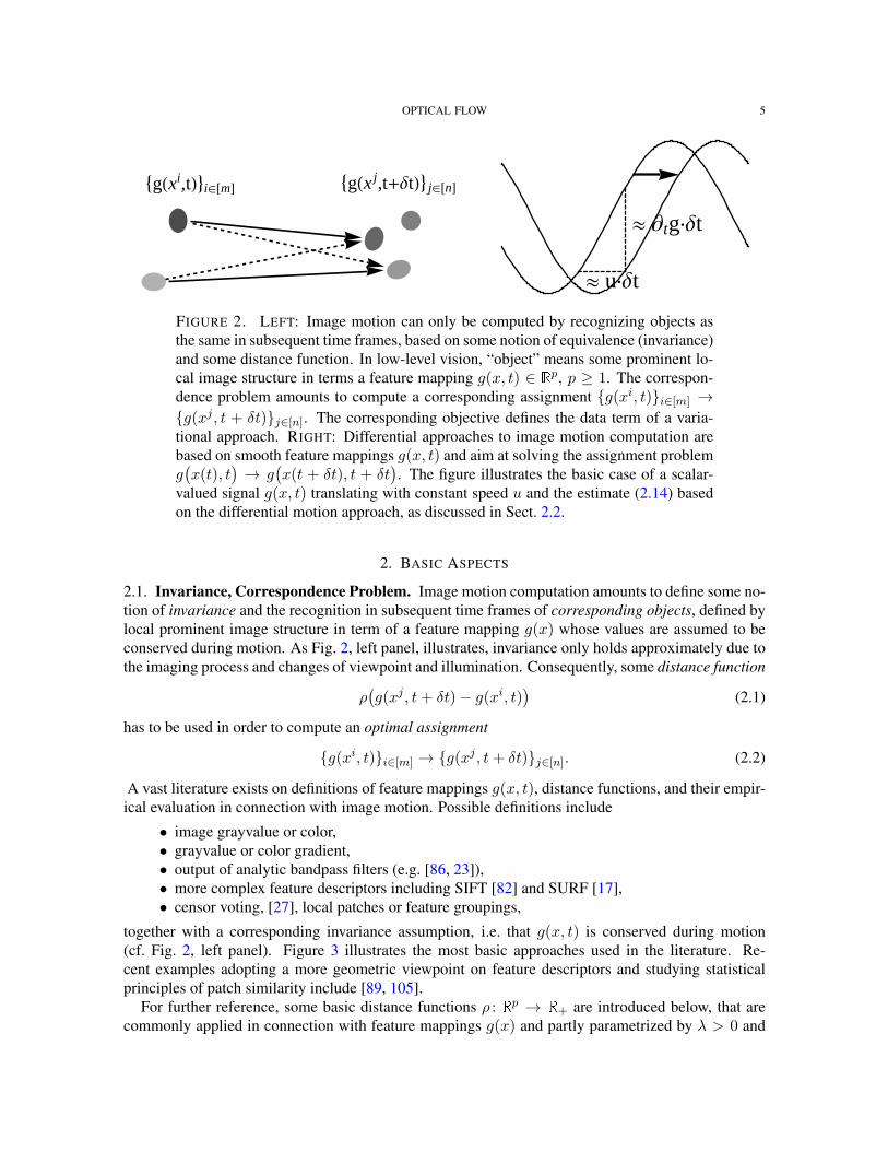
FIGURE 2. LEFT: Image motion can only be computed by recognizing objects asthe same in subsequent time frames, based on some notion of equivalence (invariance)and some distance function. In low-level vision, “object” means some prominent lo-cal image structure in terms a feature mapping g(x, t) ∈ Rp, p ≥ 1. The correspon-dence problem amounts to compute a corresponding assignment g(xi, t)i∈[m] →g(xj , t + δt)j∈[n]. The corresponding objective defines the data term of a varia-tional approach. RIGHT: Differential approaches to image motion computation arebased on smooth feature mappings g(x, t) and aim at solving the assignment problemg(x(t), t

)→ g

(x(t + δt), t + δt

). The figure illustrates the basic case of a scalar-

valued signal g(x, t) translating with constant speed u and the estimate (2.14) basedon the differential motion approach, as discussed in Sect. 2.2.

2. BASIC ASPECTS

2.1. Invariance, Correspondence Problem. Image motion computation amounts to define some no-tion of invariance and the recognition in subsequent time frames of corresponding objects, defined bylocal prominent image structure in term of a feature mapping g(x) whose values are assumed to beconserved during motion. As Fig. 2, left panel, illustrates, invariance only holds approximately due tothe imaging process and changes of viewpoint and illumination. Consequently, some distance function

ρ(g(xj , t+ δt)− g(xi, t)

)(2.1)

has to be used in order to compute an optimal assignment

g(xi, t)i∈[m] → g(xj , t+ δt)j∈[n]. (2.2)

A vast literature exists on definitions of feature mappings g(x, t), distance functions, and their empir-ical evaluation in connection with image motion. Possible definitions include

• image grayvalue or color,• grayvalue or color gradient,• output of analytic bandpass filters (e.g. [86, 23]),• more complex feature descriptors including SIFT [82] and SURF [17],• censor voting, [27], local patches or feature groupings,

together with a corresponding invariance assumption, i.e. that g(x, t) is conserved during motion(cf. Fig. 2, left panel). Figure 3 illustrates the most basic approaches used in the literature. Re-cent examples adopting a more geometric viewpoint on feature descriptors and studying statisticalprinciples of patch similarity include [89, 105].

For further reference, some basic distance functions ρ : Rp → R+ are introduced below, that arecommonly applied in connection with feature mappings g(x) and partly parametrized by λ > 0 and


(a)

(b)

(c)

(d)

(e)

(f)

(g)

FIGURE 3. (a) Lab scene ( c©CMU image database) and (b) gradient magnitude that providesthe basis for a range of feature mappings g(x, t). The image section indicated in (a)is shown in (c), and (d) shows the same section extracted from (b). Panels (e) and (f)illustrate these sections as surface plots. Panel (g) shows a feature map responding tocrossing grayvalue edges. (c), (d) and (g) correspond to the most basic examples offeature mappings g(x, t) used in the literature to compute image motion, based on acorresponding invariance assumption (cf. Fig. 2, left panel) that is plausible for videoframe rates.

0 < ε 1. For closely related functions and the nomenclature in computer vision, see e.g. [24].

ρ22(z) := ‖z‖2 squared `2 distance, (2.3a)

ρ2(z) := ‖z‖ `2 distance, (2.3b)

ρ2,ε(z) :=√‖z‖2 + ε2 − ε smoothed `2 distance, (2.3c)

ρ1(z) := ‖z‖1 `1 distance, (2.3d)

ρ1,ε(z) :=∑i∈[p]

ρ2,ε(zi) smoothed `1 distance, (2.3e)

ρ2,λ(z) := min‖z‖2, λ2 truncated squared `2 distance, (2.3f)

ρ2,λ,ε(z) := −ε log(

e−‖z‖2/ε + e−λ

2/ε)

smoothed tr. sq. `2 distance. (2.3g)

Figure 4 illustrates these convex and non-convex distance functions. Functions ρ1,ε and ρ2,ε con-stitute specific instances of the general smoothing principle to replace a lower-semicontinuous, pos-itively homogeneous and sublinear function ρ(z) by a smooth proper convex function ρε(z), withlimε0

ερε(z/ε) = ρ(z) (cf., e.g. [10]). Function ρ2,λ,ε(z) utilizes the log-exponential function [97,

Ex. 1.30] to uniformly approximate ρ2,λ as ε 0.

2.2. Assignment Approach, Differential Motion Approach.

2.2.1. Definitions. Two basic approaches to image motion computation can be distinguished.

OPTICAL FLOW 7

-1 1

1

2

-1 1

1

FIGURE 4. LEFT: Convex distance functions (2.3a)–(2.3c). CENTER: Level lines ofthe distance function ρ1,ε (2.3e). RIGHT: Non-convex distance functions (2.3f),(2.3g).

Assignment Approach, Assignment Field: This approach aims to determine an assignment offinite sets of spatially discrete features in subsequent frames of a given image sequence (Fig. 2,left panel). The vector field

u(x, t), xj = xi + u(xi, t), (2.4)

representing the assignment in Eq. (2.2), is called assignment field. This approach conformsto the basic fact that image sequences f(x, t), (x, t) ∈ Ω × [0, T ] are recorded by samplingframes

f(x, k · δt)k∈N (2.5)along the time axis.

Assignment approaches to image motion will be considered in Sect. 4.Differential Motion Approach, Optical Flow: Starting point of this approach is the invariance

assumption (Section 2.1) that observed values of some feature map g(x, t) are conserved dur-ing motion,

d

dtg(x(t), t

)= 0. (2.6)

Evaluating this condition yields information about the trajectory x(t) that represent the motionpath of a particular feature value g

(x(t)

). The corresponding vector field

x(t) =d

dtx(t), x ∈ Ω (2.7)

is called motion field whose geometric origin will be described in Sect. 2.3. Estimates

u(x, t) ≈ x(t), x ∈ Ω (2.8)

of the motion field based on some observed time-dependent feature map g(x, t), are calledoptical flow fields.

Differential motion approaches will be considered in Sect. 3.

2.2.2. Common Aspects and Differences. The assignment approach and the differential approach toimage motion are closely related. In fact, for small temporal sampling intervals,

0 < δt 1, (2.9)

one may expect that the optical flow field multiplied by δt, u(x, t) · δt, closely approximates thecorresponding assignment field. The same symbol u is therefore used in (2.4) and (2.8) to denote therespective vector fields.


A conceptual difference between both approaches is that the ansatz (2.6) entails the assumptionof a spatially differentiable feature mapping g(x, t), whereas the assignment approach requires priordecisions done at a pre-processing stage that localize the feature sets (2.2) to be assigned. The needfor additional processing in the latter case contrasts with the limited applicability of the differentialapproach: The highest spatial frequency limits the speed of image motion ‖u‖ that can be estimatedreliably:

max‖ωx‖∞, ‖u(x)‖‖ωx‖ : ωx ∈ supp g(ω), x ∈ Ω

≤ π

6. (2.10)

The subsequent section details this bound in the most simple setting for a specific but common filterchoice for estimating partial derivatives ∂ig.

2.2.3. Differential Motion Estimation: Case Study (1D). Consider a scalar signal g(x, t) = f(x, t)moving at constant speed (cf. Fig. 2, right panel),

x(t) = x = u, g(x(t), t

)= g(x(0) + ut, t

). (2.11)

Note that the two-dimensional function g(x, t) is a very special one generated by motion. Using theshorthands

x := x(0), g0(x) := g(x, 0), (2.12)g(x, t) corresponds to the translated one-dimensional signal

g(x, t) = g0(x− ut) (2.13)

due to the assumption g(x(t), t

)= g(x(0), 0

)= g0(x).

Evaluating (2.6) at t = 0, x = x(0) yields

u = − ∂tg0(x)

∂xg0(x)if ∂xg0(x) 6= 0. (2.14)

Application and validity of this equation in practice depends on two further aspects: Only sampledvalues of g(x, t) are given and the right-hand side has to be computed numericaly. Both aspects arediscussed next in turn.

(1) In practice, samples are observed

g(k · δx, tδt)k,t∈N = g(k, t)k,t∈N, δx = δt = 1, (2.15)

with the sampling interval scaled to 1 without loss of generality. The Nyquist-Shannon sam-pling theorem imposes the constraint

supp |g(ω)| ⊂ [0, π)2, ω = (ωx, ωt)> (2.16)

where

g(ω) = Fg(ω) =

∫R2

g(x, t)e−i〈ω,(xt )〉dxdt (2.17)

denotes the Fourier transform of g(x, t). Trusting in the sensor, it may be savely assumed thatsupp |g0(ωx)| ⊂ [0, π). But what about the second coordinate t generated by motion? Does itobey (2.16) such that the observed samples (2.15) truly represent the one-dimensional videosignal g(x, t)?

To answer this question, consider the specific case g0(x) = sin(ωxx), ωx ∈ [0, π] – seeFig. 5. Eq. (2.13) yields g(x, t) = sin

(ωx(x − ut)

). Condition (2.15) then requires that, for

every location x, the one-dimensional time signal gx(t) := g(x, t) satisfies supp |gx(ωt)| ⊂[0, π). Applying this to the example yields

gx(t) = sin(ωtt+ ϕ0), ωt := −ωxu, ϕ0 := ωxx, (2.18)

OPTICAL FLOW 9

FIGURE 5. A sinusoid g0(x) with angular frequency ωx = π/12, translating withvelocity u = 2, generates the function g(x, t). The angular frequency of the signalgx(t) observed at a fixed position x equals |ωt| = u ·ωx = π/6 due to (2.18). It meetsthe upper bound further discussed in connection with Fig. 6 that enables accuratenumerical computation of the partial derivatives of g(x, t).

and hence the condition

|ωt| ∈ [0, π) ⇔ |u| < π

ωx. (2.19)

It implies that equation (2.14) is only valid if, depending on the spatial frequency ωx, thevelocity u is sufficiently small.

This reasoning and the conclusion applies to general functions g(x, t), x ∈ Rd in the formof (2.10), which additionally takes into account the effect of derivative estimation, discussednext.

(2) Condition (2.19) has to be further restricted in practice, depending on how the partial deriva-tives of the r.h.s. of Eq. (2.14) are numerically computed using the observed samples (2.15).The Fourier transform

F(∂αg

)(ω) = i|α|ωαg(ω), ω ∈ Rd+1 (2.20)

generally shows that taking partial derivatives of order |α| of g(x, t), x ∈ Rd, corresponds tohigh-pass filtering that amplifies noise. If g(x, t) is vector-valued, then the present discussionapplies to the computation of partial derivatives ∂αgi of any component gi(x, t), i ∈ [p].

To limit the influence of noise, partial derivatives of the low-pass filtered feature mappingg are computed. This removes noise and smoothes the signal, and subsequent computation ofpartial derivatives becomes more accurate. Writing g(x), x ∈ Rd+1, instead of g(x, t), x ∈Rd, to simplify the following formulas, low-pass filtering of g with the impulse response h(x)

means the convolution

gh(x) := (h ∗ g)(x) =

∫Rd+1

h(x− y)g(y)dy, gh(ω) = h(ω) g(ω) (2.21)


-Π -Π

2Π

2Π

0.2

0.4

0.6

0.8

1.0

(a)

-Π -Π

2-

Π

6Π

6Π

2Π

-0.6

-0.4

-0.2

0.2

0.4

0.6

(b) (c) (d)

FIGURE 6. (a) Fourier transform hσ(ω) of the Gaussian low-pass (2.24), σ = 1. Forvalues σ ≥ 1, it satisfies the sampling condition supp |hσ(ω)| ⊂ [0, π) sufficiently ac-curate. (b) The Fourier transform of the Derivative-of-Gaussian (DoG) filter d

dxhσ(x)illustrates that for |ω| ≤ π/6 (partial) derivatives are accurately computed while noiseis suppressed at higher angular frequencies. (c), (d) The impulse responses hσ(x, t)and ∂thσ(x, t) up to size |x|, |t| ≤ 2. Application of the latter filter together with∂xhσ(x, t) to the function g(x, t) discussed in connection with Fig. 5 and evaluationof Eq. (2.14) yield the estimate u = 2.02469 at all locations (x, t) where ∂xg(x, t) 6=0.

whose Fourier transform corresponds to the multiplication of the respective Fourier trans-forms. Applying (2.20) yields

F(∂αgh

)(ω) = i|α|ωα

(h(ω) g(ω)

)=(i|α|ωαh(ω)

)g(ω). (2.22)

Thus, computing the partial derivative of the filtered function gh can be computed by convolv-ing g with the partial derivative of the impulse response ∂αh. As a result, the approximationof the partial derivative of g reads

∂αg(x) ≈ ∂αgh(x) =((∂αh) ∗ g

)(x). (2.23)

The most common choice of h is the isotropic Gaussian low-pass filter

hσ(x) :=1

(2πσ2)d/2exp

(− ‖x‖

2

2σ2

)=∏i∈[d]

hσ(xi), σ > 0. (2.24)

that factorizes (called separable filter) and therefore can be implemented efficiently. Thecorresponding filters ∂αhσ(x), |α| ≥ 1, are called Derivative-of-Gaussian (DoG) filters.

To examine its effect, it suffices to consider any coordinate due to factorization, that is theone-dimensional case. Fig. 6 illustrates that values σ ≥ 1 lead to filters that are sufficientlyband-limited so as to conform to the sampling theorem. The price to pay for effective noisesuppression however is a more restricted range supp |F

(g(x, t)

)| = [0, ωx,max], ωx,max π,

that observed image sequence functions have to satisfy, so as to enable accurate computationof partial derivatives, and in turn accurate motion estimates based on the differential approach.Figure 5 further details and illustrates this crucial fact.

2.2.4. Assignment or Differential Approach? For image sequence functions g(x, t) satisfying the as-sumptions necessary to evaluate the key equation (2.6), the differential motion approach is more con-venient. Accordingly, much work has been devoted to this line of research up to now. In particular,

OPTICAL FLOW 11

sophisticated multiscale representations of g(x, t) enable to estimate larger velocities of image mo-tion using smoothed feature mapping g (cf. Sect. 3.3.3). As a consequence, differential approachesrank top at corresponding benchmark evalutions conforming to the underlying assumptions [115] andefficient implementations are feasible [29, 55].

On the other hand, the inherent limitations of the differential approach discussed above becomeincreasingly more important in current applications, like optical flow computation for traffic scenestaken from a moving car at high speed. Figure 1, right panel, shows another challenging scenariowhere the spectral properties g(ωx, ωt) of the image sequence function and the velocity fields to beestimated render application of the differential approach difficult, if not impossible. In such cases, theassignment approach is the method of choice.

Combining both approaches in a complementary way seems most promising: robust assignmentsenable to cope with fast image motions, and a differential approach turns these estimates into spatiallydense vector fields. This point is taken up in Sect. 5.1.

2.2.5. Basic Difficulties of Motion Estimation. This section concludes with a list of some basic aspectsto be addressed by any approach to image motion computation:

(i) Definition of a feature mapping g assumed to be conserved during motion (Sect. 2.1).(ii) Coping with lack of invariance of g, change of appearance due to varying viewpoint and illumi-

nation (Sect. 3.3.1, 3.3.2).(iii) Spatial sparsity of distinctive features (Sect. 3.4).(iv) Coping with ambiguity of locally optimal feature matches (Sect. 4.2).(v) Occlusion and disocclusion of features.

(vi) Consistent integration of available prior knowledge, regularization of motion field estimation(Sect. 3.5.2, 3.5.3).

(vii) Runtime requirements (Sect. 3.6).

x

X

W

FIGURE 7. The basic pinhole model of the mathematically ideal camera. Scenepoints X are mapped to image points x by perspective projection.

2.3. Two-View Geometry, Assignment and Motion Fields. This section collects few basic relation-ships related to the Euclidean motion of a perspective camera relative to a 3D scene, that induces boththe assignment field and the motion field on the image plane, as defined in Sect. 2.2.1 by (2.4) and


(2.7). Figures 7 and 12 illustrates these relationships. References [57, 45] provide comprehensiveexpositions.

It is pointed out once more that assignment and motion fields are purely geometrical concepts.The explicit expressions (2.43) and (2.53b) illustrate how discontinuities of these fields correspondto discontinuities of depth, or to motion boundaries that separate regions in the image plane of sceneobjects (or the background) with different motions relative to the observing camera. Estimates ofeither field will be called optical flow, to be discussed in subsequent sections.

2.3.1. Two-View Geometry. Scene and corresponding image points are denoted by X ∈ R3 and x ∈R

2, respectively. Both are incident with the line λx, λ ∈ R, through the origin. Such lines are pointsof the projective plane denoted by y ∈ P2. The components of y are called homogeneous coordinatesof the image point x, whereas x and X are the inhomogeneous coordinates of image and scene points,respectively. Note that y stands for any representative point on the ray connecting x and X . In otherwords, when using homogeneous coordinates, scale factors do not matter. This equivalence is denotedby

y ' y′ ⇔ y = λy′, λ 6= 0. (2.25)

Figure 7 depicts the mathematical model of a pinhole camera with the image plane located at X3 =1. Perspective projection corresponding to this model connects homogeneous and inhomogeneouscoordinates by

x =

(x1

x2

)=

1

y3

(y1

y2

). (2.26)

A particular representative y with unknown depth y3 = X3 equals the scene point X . This reflectsthe fact that scale cannot be inferred from a single image. The 3D space R3 \ 0 corresponds to theaffine chart y ∈ P2 : y3 6= 0 of the manifold P2.

Similar to representing an image point x by homogeneous coordinates y, it is common to representscene points X ∈ R3 by homogeneous coordinates Y = (Y1, Y2, Y3, Y4)> ∈ P3, in order to linearizetransformations of 3D space. The connection analogous to (2.26) is

X =1

Y4

Y1

Y2

Y3

. (2.27)

Rigid (Euclidean) transformations are denoted by h,R ∈ SE(3) with translation vector h and properrotation matrix R ∈ SO(3) characterized by R>R = I, detR = +1. Application of the transforma-tion to a scene point X and some representative Y reads

RX + h and QY, Q :=

(R h0> 1

), (2.28)

whereas the inverse transformation −R>h,R> yields

R>(X − h) and Q−1Y, Q−1 =

(R> −R>h0> 1

). (2.29)

The nonlinear operation (2.26), entirely rewritten with homogeneous coordinates, takes the linear form

y = PY, P =

1 0 0 00 1 0 00 0 1 0

= (I3×3, 0), (2.30)

OPTICAL FLOW 13

with the projection matrix P and external or motion parameters h,R. In practice, additional inter-nal parameters characterizing real cameras to the first order of approximation are taken into accountin terms of a camera matrix K and the corresponding modification of (2.30),

y = PY, P = K(I3×3, 0). (2.31)

As a consequence, the transition to normalized (calibrated) coordinates

y := K−1y (2.32)

corresponds to an affine transformation of the image plane.Given an image point x, taken with a camera in the canonical position (2.30), the corresponding ray

meets the scene point X , see Figure 12 (b). This ray projects in a second image, taken with a secondcamera positioned by h,R relative to the first camera and with projection matrix

P ′ = K ′R>(I,−h), (2.33)

to the line l′, on which the projection x′ of X corresponding to x must lie. Turning to homogeneouscoordinates, an elementary computation shows that the fundamental matrix

F := K ′−>R>[h]×K−1 (2.34)

maps y to the epipolar line l′,l′ = Fy. (2.35)

This relation is symmetrical in that F> maps y′ to the corresponding epipolar line l in the first image,

l = F>y′. (2.36)

The epipoles e, e′ are the image points corresponding to the projection centers. Because they lie on land l′ for any x′ and x, respectively, it follows that

Fe = 0, F>e′ = 0. (2.37)

The incidence relation x′ ∈ l′ algebraically reads 〈l′, y′〉 = 0. Hence by (2.35),

〈y′, Fy〉 = 0 (2.38)

This key relation constrains the correspondence problem x ↔ x′ for arbitrary two views of the sameunknown scene point X . Rewriting (2.38) in terms of normalized coordinates by means of (2.32)yields

〈y′, Fy〉 = 〈K ′−1y′,K ′>FK(K−1y)〉 = 〈K ′−1y′, E(K−1y)〉 (2.39)with the essential matrix E that, due to (2.34) and the relation [Kh]× ' K−>[h]×K

−1, is given by

E = K ′>FK = R>[h]×. (2.40)

Thus, essential matrices are parametrized by transformations h,R ∈ SE(3) and therefore form asmooth manifold embedded in R3×3.

2.3.2. Assignment Fields. Throughout this section, the internal camera parameters K are assumed tobe known and hence normalized coordinates (2.32) are used. As a consequence,

K = I (2.41)

is set in what follows.Suppose some motion h,R of a camera relative to a 3D scene causes the image point x of a fixed

scene pointX to move to x′ in the image plane. The corresponding assignment vector u(x) representsthe displacement of x in the image plane,

x′ = x+ u(x), (2.42)


which due to (2.29) and (2.26) is given by

u(x) =1

〈r3, X − h〉

(〈r1, X − h〉〈r2, X − h〉

)− 1

X3

(X1

X2

). (2.43)

Consider the special case of pure translation, i.e. R = I, ri = ei, i = 1, 2, 3. Then

u(x) =1

X3 − h3

(X1 − h1

X2 − h2

)− 1

X3

(X1

X2

)(2.44a)

=1

h3 − 1

((h1

h2

)− h3

(x1

x2

)), h :=

1

X3h. (2.44b)

The image point xe where the vector field u vanishes, u(xe) = 0, is called focus of expansion (FOE)

xe =1

h3

(h1

h2

). (2.45)

xe corresponds to the epipole y = e since Fe ' R>[h]×h = 0.Next the transformation is computed of the image plane induced by the motion of the camera in

terms of projection matrices P = (I, 0) and P ′ = R>(I,−h) relative to a plane in 3D space

〈n,X〉 − d = n1X1 + n2X2 + n3X3 − d = 0, (2.46)

with unit normal n, ‖n‖ = 1, and with signed distance d of the plane from the origin 0. Settingp = ( n

−d ), Eq. (2.46) reads〈p, Y 〉 = 0. (2.47)

In order to compute the point X on the plane satisfying (2.46) that projects to the image point y, theray Y (λ) =

(λy1

), λ ∈ R, is intersected with the plane.

〈p, Y (λ)〉 = λ〈n, y〉 − d = 0 ⇒ λ =d

〈n, y〉, Y =

( d〈n,y〉y

1

)'(

y1d〈n, y〉

). (2.48)

Projecting this point onto the second image plane yields

y′ = P ′Y (λ) = R>(y − 1

d〈n, y〉h

)= R>(I − 1

dhn>)y

=: Hy

(2.49)

Thus, moving a camera relative to a 3D plane induces a homography (projective transformation) H ofP

2 which by virtue of (2.26) yields an assignment field u(x) with rational components.

2.3.3. Motion Fields. Motion fields (2.7) are the instantaneous (differential) version of assignmentfields. Consider a smooth path h(t), R(t) ⊂ SE(3) through the identity 0, I and the correspond-ing path of a scene point X ∈ R3

X(t) = h(t) +R(t)X, X = X(0). (2.50)

Let R(t) be given by a rotational axis q ∈ R3 and a rotation angle ϕ(t). Using Rodrigues’ formula

and the skew-symmetric matrix [q]× ∈ so(3) with ϕ = ϕ(0) := ‖q‖, matrix R(t) takes the form

R(t) = exp(t[q]×) = I +sin(ϕt)

ϕtt[q]× +

1− cos(ϕt)

(ϕt)2t2[q]2×. (2.51)

(2.50) then yieldsX(0) = v + [q]×X, v := h(0), (2.52)

OPTICAL FLOW 15

where v is the translational velocity at t = 0. Differentiating (2.26) with y = X (recall assumption(2.41)) and inserting (2.52), gives

d

dtx =

1

X23

(X3X1 −X1X3

X3X2 −X2X3

)=

1

X3

(X1 − x1X3

X2 − x2X3

)(2.53a)

=1

X3

[(v1

v2

)− v3

(x1

x2

)]+

(q2 − q3x2 − q1x1x2 + q2x

21

−q1 + q3x1 + q2x1x2 − q1x22

). (2.53b)

Comparing (2.53b) to (2.43) and (2.44b) shows a similar structure of the translational part with FOE

xv :=1

v3

(v1

v2

), (2.54)

whereas the rotational part merely contributes an incomplete second-order degree polynomial to eachcomponent of the motion field, that do not depend on the scene structure in terms of the depth X3.

Consider the special case of a motion field induced by the relative motion of a camera to a 3D planegiven by (2.46) and write

1

X3=

1

d

(n3 +

(n1

n2

)>(x1

x2

)). (2.55)

Insertion into (2.53b) shows that the overall expression for the motion fields takes a simple polynomialform.

2.4. Early Pioneering Work. It deems proper to the authors to refer at least briefly to early pio-neering work related to optical flow estimation, as part of a survey paper. The following referencesconstitute just a small sample of the rich literature.

The information of motions fields, induced by the movement of an observer relative to a 3D scene,was picked out as a central theme more than three decades ago [81, 95]. Kanatani [72] studied therepresentation of SO(3) and invariants in connection with the space of motion fields induced by themovement relative to a 3D plane. Approaches to estimating motion fields followed soon, by deter-mining optical flow from local image structure [84, 91, 63, 133, 131, 132]. Poggio and Verri [122]pointed out both the inexpedient, restrictive assumptions making the invariance assumption (2.6) holdin the simple case g(x) = f(x) (e.g. Lambertian surfaces in the 3D scene), and the stability of struc-tural (topological) properties of motion fields (like e.g. the FOE (2.45)). The local detection of imagetranslation as orientation in spatio-temporal frequency space, based on the energy and the phase ofcollections of orientation-selective complex-valued bandpass filters (lowpass filters shifted in Fourierspace, like e.g. Gabor filters), was addressed by [2, 60, 46], partially motivated by related research onnatural vision systems.

The variational approach to optical flow was pioneered by Horn and Schunck [68], followed byvarious extensions [92, 6, 144] including more mathematically oriented accounts [109, 64, 130]. Thework [129] classified various convex variational approaches that have unique unique minimizers.

The computation of discontinuous optical flow fields, in terms of piecewise parametric represen-tations, was considered by [128, 24], whereas the work [118] studied the information contained incorrespondences induced by motion fields over a longer time period. Shape-based optimal control offlows determined on discontinuous domains as control variable, was introduced in [110], includingthe application of shape derivative calculus that became popular later on in connection with level sets.Markov random fields and the Bayesian viewpoint on the non-local inference of discontinuous opticalflow fields were introduced in [62]. The challenging aspects of estimating both motion fields and theirsegmentation in a spatio-temporal framework, together with inferring the 3D structure, has remaineda topic of research until today.


This brief account shows that most of the important ideas appeared early in the literature. On theother hand, it took many years until first algorithms made their way into industrial applications. A lotof work remains to be done by addressing various basic and applied research aspects. In comparisonto the fields of computer vision, computer science and engineering, not much work has been done bythe mathematical community on motion based image sequence analysis.

2.5. Benchmarks. Starting with the first systematic evaluation in 1994 by Baron et al. [15], bench-marks for optical flow methods have stimulated and steered the developement of new algorithms inthis field. The Middlebury database [14] further accelerated this trend by introducing an online rank-ing system and defining challenging data sets, which specifically address different aspects of flowestimation such as large displacements or occlusion.

The recently introduced KITTI Vision Benchmark Suite [47] concentrates on outdoor automotivesequences that are affected by disturbances such as illumination changes and reflections, which opticalflow approaches are expected to be robust against.

While real imagery requires sophisticated measurement equipment to capture reliable referenceinformation, synthetic sequences such as the novel MPI Sintel Flow Dataset [32] come with freeground truth. However, enormous efforts are necessary to realistically model the scene complexityand effects found in reality.

OPTICAL FLOW 17

3. THE VARIATIONAL APPROACH TO OPTICAL FLOW ESTIMATION

In contrast to assignment methods, variational approaches to estimating the optical flow employ acontinuous and dense representation of the variables u : Ω 7→ R

2. The model describing the agree-ment of u with the image data defines the data term ED(u). It is complemented by a regularizationterm ER(u) encoding prior knowledge about the spatial smoothness of the flow. Together these termsdefine the energy function E(u) and estimating the optical flow amounts to finding a global mini-mum u, possibly constrained by a set U of admissible flow fields, and using an appropriate numericalmethod:

infu∈U

E(u) , E(u) := ED(u) + ER(u) (3.1)

E(u) is non-convex in general and hence only suboptimal solutions can be determined in practice.Based on the variational approach published in 1981 by Horn & Schunck [68] a vast number of

refinements and extensions were proposed in literature. Recent comprehensive empirical evaluations[47, 14] reveal that algorithms of this family yield best performance. Section 3.2 introduces the ap-proach of Horn and Schunck as reference for the following discussion, after deriving the requiredlinearized invariance assumption in Sect. 3.1.

Data and regularization terms designed to cope with various difficulties in real applications arepresented in Sections 3.3 and 3.4, respectively. Section 3.6 gives a short overview over numerical al-gorithms for solving problem (3.1). Section 3.5 addresses some important extensions of the discussedframework.

3.1. Differential Constraint Equations, Aperture Problem. All variational optical flow approachesimpose an invariance assumption on some feature vector g(x, t) ∈ R

p, derived from an image se-quence f(x, t) as discussed in Sect. 2.1. Under perfect conditions, any point moving along the trajec-tory x(t) over time t with speed u(x, t) := d

dtx(t) does not change its appearance, i.e.

d

dtg(x(t), t) = 0 . (3.2)

Without loss of generality, motion at t = 0 is considered only in what follows. Applying the chainrule and dropping the argument t = 0 for clarity, leads to the linearized invariance constraint,

Jg(x)u(x) + ∂tg(x) = 0 . (3.3)

Validity of this approximation is limited to displacements of about 1 pixel for real data as elaboratedin Sect. 2.2.2, which seriously limits its applicability. However, Sect. 3.3.3 describes an approach toalleviating this restriction and thus for now it is safe to assume that the assumption is fulfilled.

A least squares solution to (3.3) is given by (S(x))−1(J>g (x)(∂tg(x))) where

S(x) := J>g (x) Jg(x). (3.4)

However, in order to understand the actual information content of equation system (3.3), the locallyvarying properties of the Jacobian matrix Jg(x) have to be examined:

rank(Jg) = 0: void constraints on u(x) (for g(x, 0) = const.);

rank(Jg) = 1: ill-conditioned constraints, a single component of u(x) is determined only;

p = rank(Jg) = 2: unique solution u(x) = − J−1g (x)(∂tg(x));

p > rank(Jg) = 2: over-determined and possibly conflicting constraints on u(x), cf. Fig. 8.

In the case of gray-valued features g(x) = f(x) ∈ R, (3.3) is referred to as the linearized brightness


(a) syntheticscenarios

(b) real image data (c) local information content

FIGURE 8. Ellipse representation of S = J>g Jg as in (3.2) for a patch feature vectorwith p 2 (see Sect. 3.3.2). (a) Three synthetic examples with Jg having (top tobottom) rank 0, 1 and 2, respectively. (b) Real image data with homogeneous (left)and textured (right) region, image edges and corner (middle). (c) Locally varyinginformation content (see Sect. 3.1) of the path features extracted from (b).

constancy constraint and imposes only one scalar constraint on u(x) ∈ R2, in the direction of the

image gradient Jg(x) = (∇g(x))> 6= 0, i.e.⟨∇g(x)

‖∇g(x)‖, u(x)

⟩= − ∂tg(x)

‖∇g(x)‖. (3.5)

This limitation which only allows to determine the normal flow component is referred to as the aper-ture problem in the literature.

Furthermore, for real data, invariance assumptions do not hold exactly and compliance is measuredby the data term as discussed in Sect. 3.3. Section 3.4 addresses regularization terms which furtherincorporate regularity priors on the flow so as to correct for data inaccuracies and local ambiguitiesnot resolved by (3.3).

3.2. The Approach of Horn & Schunck. The approach by Horn & Schunck [68] is described in thefollowing due to its importance in the literature, its simple formulation and the availability of wellunderstood numerical methods for efficiently computing a solution.

3.2.1. Model. Here the original approach [68], expressed using the variational formulation (3.1), isslightly generalized from gray-valued features g(x) = f(x) ∈ R to arbitrary feature vectors g(x) ∈Rp. Deviations from the constancy assumption in (3.3) are measured using a quadratic function ρD =ρ2

2, leading to

ED(u) =1

2

∫ΩρD

(‖Jg(x)u(x) + ∂tg(x)‖F

)dx . (3.6)

As for regularization, the quadratic length of the flow gradients is penalized using ρR = ρ22, to enforce

smoothness of the vector field and to overcome ambiguities of the data term (e.g. aperture problem;see Sect. 3.1):

ER(u) =1

2σ2

∫ΩρR(‖ Ju(x)‖F )dx . (3.7)

The only parameter σ > 0 weights the influence of regularization against the data term.

OPTICAL FLOW 19

3.2.2. Discretization. Finding a minimum of E(u) = ED(u) + ER(u) using numerical methodsrequires discretization of variables and data in time and space. To this end, let xii∈[n] define aregular two-dimensional grid in Ω, and let g1(xi) and g2(xi) be the discretized versions of g(x, 0) andg(x, 1) of the input image sequence, respectively. Motion variables u(xi) are defined on the same gridand stacked into a vector u:

u(xi) =(u1(xi)

u2(xi)

), u =

((u1(xi))i∈[n]

(u2(xi))i∈[n]

)∈ R2n. (3.8)

The appropriate filter for the discretization of the spatial image gradients ∂ig strongly depends onthe signal and noise properties as discussed in Sect. 2.2.3. A recent comparison [115] reports that a5-point derivative filter ( 1

12−1, 8, 0,−8, 1) applied to 12(g1 +g2) performs best. Temporal gradients

are approximated as ∂tg(xi) ≈ g2(xi)− g1(xi).As a result, the discretized objective function can be rewritten as

E(u) =1

2‖Du+ c‖2 +

1

2σ2‖Lu‖2 , (3.9)

using the linear operators

D :=

(D1,1 D1,2

......

Dp,1 Dp,2

), c :=

(c1...cp

), L :=

( L1,1

L1,2

L2,1

L2,2

), (3.10)

with data derivatives cj := (∂tgj(xi))i∈[n] and Dj,k := diag

((∂kgj(x

i))i∈[n]

). The matrix opera-

tor Ll,k applied to variable u approximates the spatial derivative ∂k of the flow component ul usingthe 2-tap linear filter −1,+1 and Neumann boundary conditions.

3.2.3. Solving. Objective function (3.9) is strictly convex in u under mild conditions [109] and thusa global minimum of this problem can be determined by finding a solution to ∇uE(u) = 0. Thiscondition explicitly reads

(D>D + σ−2L>L)u = −D>c (3.11)

which is a linear equation system of size 2n in u ∈ R2n with a positive definite and sparse matrix. Anumber of well-understood iterative methods exist to efficiently solve this class of problems even forlarge n [104].

3.2.4. Examples. Figure 9 illustrates the method by Horn & Schunck for a small synthetic example.The choice of parameter σ is a trade-off between smoothing out motion boundaries (see Fig. 9(b)) inthe true flow field (Fig. 9(a)) and sensitivity to noise (Fig. 9(d)).

3.2.5. Probabilistic Interpretation. Considering E(u) as a the log-likelihood function of a probabil-ity density function gives rise to the maximum a-posteriori interpretation of the optimization prob-lem (3.1), i.e.

supu∈U

p(u |g, σ ) , p(u |g, σ ) ∝ exp(−E(u)) . (3.12)

As E(u) is quadratic and positive definite due to the assumptions made in Sect. 3.2.3, this posterior isa Gaussian multivariate distribution

p(u |g, σ ) = N (u;µ,Σ) (3.13)

with precision (inverse covariance) matrix Σ−1 = D>D+σ−2L>L and mean vector µ = −Σ−1D>cthat solves (3.11).


(a) correct flow (b) estimated flow, σ2 = 102 (c) estimated flow, σ2 = 103 (d) estimated flow, σ2 = 104

FIGURE 9. (a) Synthetic flow field used to deform an image. (b)–(d) Flow field es-timated by the approach by Horn & Schunck with decreasing strength of the smooth-ness prior.

Examining the conditional distribution of ui ∈ R2 allows to quantify the sensitivity of u. To this

end a permutation matrix Q =

(QiQi

)∈ R2n×2n, Q>Q = I , is defined such that ui = Qiu. Then,

fixing Qiu = Qiµ leads to

p(ui∣∣Qiu) = N

(µi, Σi

)(3.14)

with µi = Qiµ andΣi = QiΣQ

>i − (QiΣQ

>i )(QiΣQ

>i

)−1(QiΣQ>i

) . (3.15)Using the matrix inversion theorem to invert Σ block-wise according to Q and restricting the resultto ui, reveals

QiΣ−1Qi =

(QiΣQ

>i − (QiΣQ

>i )(QiΣQ

>i

)−1(QiΣQ>i

))−1

. (3.16)

Comparison of (3.15) to (3.16) and further analysis yields (for non-boundary pixels)

Σi =(QiΣ

−1Qi)−1

=(Si + 4σ−2I

)−1(3.17)

with Si = S(xi) as defined by (3.4). Consequently, smaller values of σ reduce the sensitivity of ui,but some choice σ > 0 is inevitable for singular Si.

3.3. Data Terms.

3.3.1. Handling Violation of the Constancy Assumption. The data term as proposed by Horn & Schunckwas refined and extended in literature in several ways with the aim to cope with the challenging prop-erties of image data of real applications, see Sect. 2.2.5.

Changes of the camera viewpoint as well as moving or transforming objects may cause previouslyvisible image features to disappear due to occlusion, or vice versa to emerge (dis-occlusion), leadingto discontinuous changes of the observed image features g(x(t), t) over time and thus to a violationof the invariance constraint (3.2).

Surface reflection properties like specular reflections that vary as the viewpoint changes, and vary-ing emission or illumination (including shadows) also cause appearance to change, in particular innatural and outdoor scenes.

With some exceptions, most approaches do not to explicitly model these cases and instead replacethe quadratic distance function ρ2

2 by the convex `2-distance or its differentiable approximation ρ2,ε,to reduce the impact of outliers in regions with strong deviation from the invariance assumption. A

OPTICAL FLOW 21

number of non-convex alternatives have been proposed in the literature, including the truncated squaredistance ρ2,λ, which further extend this concept and are often referred to as “robust” approaches.

Another common method is to replace the constancy assumption on the image brightness by oneof the more complex feature mappings g(x, t) introduced in Sect. 2.1, or combinations of them. Theaim is to gain more descriptive features that overcome the ambiguities described in Sect. 3.1, e.g. byincluding color or image structure information from a local neighborhood. Furthermore, robustness ofthe data term can be increased by choosing features invariant to specific image transformations. Forexample, g(x) = ∇f(x) is immune to additive illumination changes.

3.3.2. Patch Features. Contrary to the strongly localized brightness feature g(x) = f(x), local imagepatches sampled from a neighborhood N (x) of x,

g(xi, t) =(f(xj , t)

)xj∈N (xi)

∈ Rp, p = |N (xi)| (3.18)

provide much more reliable information on u in textured image regions. In fact, local approaches setER(u) = 0 and rely only the information contained in the data term.

The most prominent instance introduced by Lucas & Kanade [84], chooses a Gaussian weightedquadratic distance function,

ρ2wi(z) := ‖diag(wi)

12 z‖2 , wi := (w(xi − xj))xj∈N (xi) (3.19)

and w(x) := exp(−‖x‖2/(2σ2)

). Solving the variational problem (3.1) decomposes into n linear

systems of dimension 2 each. Furthermore, the sensitivity in terms of (3.17) reduces to Σi = (Si)−1

andSi =

∑xj∈N (xi)

w(xi − xj)(

J>g (xj) Jg(xj))

(3.20)

equals the so-called structure tensor. At locations with numerically ill-conditioned Jg, cf. Fig. 8 andthe discussion in Sect. 3.1, no flow can be determined reliably which leads to possibly sparse results.The works [111, 30] overcome this drawback by complementing this data term by a regularizationterm.

3.3.3. Multiscale. As discussed in Sect. 2.2.3, the range of displacements u(x) that can be accuratelyestimated, is limited to about 1 pixel which does not conform to the larger magnitude of motion fieldstypically encountered in practical applications. Multiscale methods allow to remove this restriction tosome extent. They implement a coarse-to-fine strategy for approximately determining large displace-ments on spatially band-limited image data and complementing flow details on finer scales.

The underlying idea is introduced by means of a multiscale representation g[l]l∈[nl] of image data,where l = 0 and l = nl − 1 refer to the finest and coarsest scale, respectively. More precisely, g[l]

is a spatially band-limited version of g with ωx,max < slπ with 1 = s0 > s1 · · · snl−1 > 0. Thecomputation is described by the following recursive scheme with u[nl](x) = 0:

• g[l](x, t) := hl ∗ g(x+ t · u[l+1], t)

• δu[l] := arg minuE(u) on data g[l](x, t)

• u[l](x) := u[l+1](x) + δu[l](x)

with a suitable approximation of the ideal low-pass filter hl with frequency response

hl(ωx, ωt) ≈

1 ‖ωx‖∞ < slπ

0 otherwise. (3.21)

Figure 10 demonstrates the method for two simple examples.


0 50 100 150 200 2500

0.2

0.4

0.6

0.8

1

x

g[l](x,0)

(a) multiscale data

0 50 100 150 200 25023

23.2

23.4

23.6

23.8

24

x

u[l] (x)

(b) multiscale flow

0 50 100 150 200 250 300 350 400 450 5000

0.2

0.4

0.6

0.8

1

x

g[l](x,0)

(c) multiscale data

0 50 100 150 200 250 300 350 400 450 50023

23.5

24

24.5

25

x

u[l] (x)

(d) multiscale flow

FIGURE 10. Multiscale flow estimation: (a) An image (white noise) g[l](x, 0) rep-resented at multiscale levels l = 0 (black), l = 3 (blue), l = 6 (red) with sl = 2−l,i.e. band-limited to slπ. (b) Estimate u[l] (same color encoding as in (a)) of correctconstant flow u(x) = 23.3 on multiscale level l. (c)-(d) Same as (a)-(b) for a singleline of a real image ( c©LaVision GmbH) as found in particle image velocimetry, an opticalfluid flow estimation method.

Actual implementations further make use of the band-limited spectrum of the filtered data and sub-sample the data according to the Nyquist-Shannon sampling theorem, leading to a data representationreferred to as resolution pyramid. The recursive structure allows in turn to approximate hl by chainingfilters with small support for computational efficiency.

3.4. Regularization. Ill-posed data terms, sensor noise and other distortions lead to sparse and lo-cally inaccurate flow estimates. Variational approaches allow to incorporate priors on the motionregularity by means of additional terms ER(u). For suitable models ED(u) and ER(u), accuracyprofits from this concept as the global solution to minimization problem (3.1) represents the best flowfield according to both observations and priors. Furthermore, in contrast to local methods, missingflow information is approximately inferred according to the smoothness prior. This is in particularessential in connection with ill-posed data terms (cf. Sect. 3.1).

3.4.1. Regularity Priors. A number of a-priori constraints u ∈ U for flow estimation have beenproposed in the literature, based on prior knowledge specific to the application domain. Examplesinclude

• inherent geometrical constraints induced by multi-camera setups (Sect. 3.5.2),• physical properties of flows in experimental fluid mechanics (Sect. 3.5.3).

OPTICAL FLOW 23

(a) correct flow (b) estimated flow, σ2 = 102 (c) estimated flow, σ2 = 103 (d) estimated flow, σ2 = 104

FIGURE 11. (a) Synthetic flow field used to deform an image. (b)–(d) Flow fieldestimated by the approach by Horn & Schunck, however with `1−TV -regularization,with decreasing strength of the smoothness prior.

Formally, strict compliance with a constraint u ∈ U can be incorporated into the variational formula-tion (3.1) by means of the corresponding indicator function

ER(u) = δU (u) . (3.22)

In many applications, however, the set U cannot be specified precisely. Then a common approach isto replace δU by a smoother function measuring the distance of u to U in some sense,

ER(u) = ρ(u−ΠUu). (3.23)

For example, the regularization term of the Horn & Schunck approach presented in Sect. 3.2 may bewritten as

ER(u) = ‖Lu‖2 = ‖u−Πker(L)(u)‖2L (3.24)with semi-norm ‖x‖L := ‖Lx‖ and set U = ker(L). Generalizations of the approach of Horn &Schunck are based on the same L and modify the distance function (Sect. 3.4.2) or refine them tobecome locally adaptive and anisotropic (Sect. 3.4.3).

Further extensions replace the gradient operator in (3.7) and its discretization L by other opera-tors having a larger space U = ker(L). For example, operators involving second order derivatives∇ div and ∇ curl have been used for flow estimation in experimental fluid dynamics [141, 142, 143](cf. Sect. 3.5.3).

3.4.2. Distance Functions. Occlusion of objects do not only lead to sudden changes of the projectedappearance (cf. Sect. 3.3), but also to motion discontinuities whose preservation during flow estimationis crucial in many applications and for the interpretation of videos. The penalization of large motiongradients Ju can be reduced by replacing the quadratic distance function ρ2

2 in (3.7) by convex ornon-convex alternatives, see (2.3) for some examples.

Figure 11 demonstrates the effect of replacing the quadratic distance measure of the approach byHorn & Schunck (Sect. 3.2) by ρR = ρ2. It becomes apparent that motion discontinuities can be betterresolved than with ρR = ρ2

2 (see Fig. 9).

3.4.3. Adaptive, Anisotropic and Non-local Regularization. A further option is to include a-prioriinformation on the location and alignment of motion discontinuities by using a spatially varying,adaptive and possibly anisotropic norm in (3.7),

ER(u) = σ−2

∫ΩρR(‖ Ju(x)‖W (x))dx , (3.25)


with ‖A‖W := ‖AW‖F and (omitting the dependency on x)

W =(w1e

1 w2e2). (3.26)

The normalized orthogonal directions e1, e2 ∈ R2 point across and along the assumed motion bound-ary, respectively. The positive eigenvalues w1 and w2 control relative penalization of flow changes inthe according direction.

A common assumption made in literature, e.g. [134, 129], is that image edges and flow disconti-nuities coincide and to facilitate changes of u(x) across the assumed boundary e1. For general fea-tures g(x), the notion of image edge is here defined by choosing e1 and e2 as the normalized direction eof the largest and smallest change of ‖ Jg e‖, respectively, given by the eigenvectors of S = J>g Jg. Theassociated eigenvalues λ1 ≥ λ2 ≥ 0 of S control the strength of smoothness by settingwi = 1−ρ(λi),i = 1, 2 and suitable increasing ρ(x) ∈ [0, 1] with ρ(0) = 0. This defines an anisotropic and image-driven regularization. Note that for the gray-valued case g(x) = f(x) ∈ R the formulation simplifiesto e1 = ‖∇g‖−1∇g, λ1 = ‖∇g‖2 and λ2 = 0. The class of flow-driven approaches replace thedependency on g(x) of the terms above by the flow u(x) to be estimated. This nonlinear dependencycan be taken into account without compromising convexity of the overall variational approach [129].

While the approaches so far measure locally the regularity of flows u, approaches such as [79] adoptnon-local functionals for regularization developed in other contexts [76, 48, 44] for optical flow esti-mation. Regularization is then more generally based on the similarity between all pairs (u(x), u(x′))with x, x′ ∈ Ω, weighted by mutual position and feature distances.

3.5. Further Extensions. Three extensions of the basic variational approach are sketched: a naturalextension of spatial regularizers to the spatio-temporal domain (Sect. 3.5.1), regularization based onthe two-view geometry (cf. Sect. 2.3) and relative rigid motions for computer vision applications(Sect. 3.5.2) and a case study of PDE-constrained variational optical flow estimation in connectionwith imaging problems in experimental fluid dynamics (Sect. 3.5.3).

3.5.1. Spatio-Temporal Approach. The preceding discussion reduced the motion estimation problemto determining displacements between two image frames only and thus ignored consistencies of theflow over time. Although in many applications recording rates are fast compared to dynamical changesdue to modern sensors, only few approaches exploit this fact by introducing temporal smoothnesspriors.

The work [130] proposed to process a batch of image frames simultaneously and to extend the flowfield domain along the time axis u : Ω × [0, T ] 7→ R

2. While data terms are independently imposedfor each time t, the smoothness prior is extended by a temporal component to

ER(u) :=

∫Ω×[0,T ]

ρR(‖ Ju,t(x, t)‖W )dxdt . (3.27)

Here, Ju,t represents the spatio-temporal derivatives and ρR‖ · ‖W is a three-dimensional extension ofthe anisotropic, flow-driven distance function discussed in Sect. 3.4.3. It allows to account for smallposition changes of moving objects between consecutive frames within the support of the regulariza-tion term (≤ 1 px) by supporting smoothness along an assumed trajectory.

Larger displacements, however, require matching of temporally associated regions e.g. using a mul-tiscale framework (Sect. 3.3.3) but then enable to regularize smoothness of trajectories over multipleframes as proposed in [126].

Online methods are an appealing alternative whenever processing a batch of image frames is notfeasible due to resource limitations. This approach is addressed in Sect. 5.3.

OPTICAL FLOW 25

xx′ = x+ u

camera at t = 1

camera at t = 0

Q

X

(a) optical flow induced by camera motion

x

e e′

x′

epipolar plane

l′

camera at t = 0 camera at t = 1

X

(b) epipolar constraint

FIGURE 12. (a) Relative motion Q ∈ SE(3) of the camera w.r.t. a world coordinatesystem causes the projection x of a static scene point X = z(x)y to move from x tox′ = x + u(x) in the image plane. (b) Any two projections x, x′ of a scene point Xare related by the essential matrix E as in (3.29), defining an epipolar plane andtheir projection, the epipolar lines defined by x, e and x′, e′ in the image planeat t = 0 and t = 1, respectively.

3.5.2. Geometrical Prior Knowledge. In applications with a perspective camera as image sensor, thegeometrical scene structure strongly determines the observed optical flow (Sect. 2.3). This sectionbriefly addresses the most common assumptions made and the constraints that follow.

Often, a static scene assumption is made, meaning that all visible scene points have zero velocitywith respect to a world coordinate system. Then the observed motion is only induced by the cameramoving in the scene. Using the notation introduced in Sect. 2.3, the camera motion is denoted by Q ∈SE(3) (cf. Fig. 12(a)), parametrized by rotation R ∈ SO(3) and translation h ∈ R3, so that any scenepoint Y ∈ is transported to Y ′ ' Q−1Y .

The following discussion of common setups and their implications on the observed motion implic-itly assumes that the scene point is visible in both frames. Using assumption (2.41) for the internalcamera parameters allows to work with normalized coordinates (2.32). The point corresponding to xis denoted by x′, due to (2.42).

Static scene, general motion: Let the depth map z(x) : Ω 7→ R parametrize the scene pointX := z(x) ( x1 ) visible at x in the camera plane in the first frame. Then the projected corre-spondences are given in homogeneous coordinates by

y′ ' PQ−1Y = R> (z(x) ( x1 )− h) , (3.28)

see Fig. 12(a) for an illustration. Figure 13 shows the optical flow field u(x) conforming toconstraint (3.28) for a real application.

It is possible to eliminate the dependency on z(x), that typically is unknown, by means ofthe essential matrix E := R>[h]×, leading to the epipolar constraint

(y′)>Ey = 0 , (3.29)


(a) frame from a real image se-quence

(b) estimated flow u(x) and color code

far

near

(c) estimated depth z(x)

FIGURE 13. (a) A single frame from an image sequence recorded by a camera mov-ing forward through an approximately static scene. (b) Optical flow estimated usingthe parametrization u(x) = u(x;Q, z(x)) according to (3.28) and global optimiza-tion for Q ∈ SE(3), z ∈ Rn, see [18] for details. Displacement length and directionare encoded by saturation and hue, respectively, see color code on the right. (c) Esti-mated depth parameter z(x) using the color code on the right. Scene structure is moreevident in this representation and therefore the spatial smoothness prior on the flowwas formulated as regularization term on the depth z(x) instead of displace-ments u(x).

as illustrated by Fig. 12(b). This gives rise to an orthogonal decomposition [112] of an ob-served correspondence x′ into

x′ = x′e + x′⊥ (3.30)

with x′e fulfilling (3.29) and orthogonal deviations x′⊥.Even without knowing a-priori (R, h), equation (3.29) provides a valuable prior: Valgaerts

et al. [121] propose joint computation of the fundamental matrix F related to E by (2.40) andoptical flow constrained via (3.29). They show that estimation of F is more stable and thatflow accuracy is significantly increased.

Static scene, coplanar camera motion: If the camera translates parallel to the image plane only,i.e. R = I and h =

(b0

)with b ∈ R

2, the observed flow is constrained to a locally varyingone-dimensional subspace parametrized by the inverse depth,

u(x) = z−1(x)b . (3.31)

Stereoscopic camera setups fulfill the static scene assumption as they can be interpreted as aninstantaneous camera motion with baseline ‖b‖. For details see e.g. [27].

Planar and static scene, general camera motion: In applications where the scene can be (lo-cally) approximated by a plane such that 〈n,X〉 − d = 0 for all space points X with planeparameters d, n as in (2.46), all correspondences fulfill

y′ ' Hy, H = R>(I − 1

dhn>

), (3.32)

where H ∈ R3×3 defines a homography – cf. Eq. (2.49).

3.5.3. Physical Prior Knowledge. Imaging of dynamic phenomena in natural sciences encountersoften scenarios where physical prior knowledge applies. Examples include particle image velocime-try [3] or Schlieren velocimetry [8], where the motion of fluids is observed that is governed by physical

OPTICAL FLOW 27

laws. While local methods such as cross-correlation methods are commonly used to evaluate the ob-tained image sequences [135, 3], variational approaches [100, 101, 61] provide a more appropriatemathematical framework for exploiting such prior knowledge and the estimation of physically consis-tent optical flows.

For instance the Helmholtz decomposition of vector fields enables to define regularizers in termsof higher-order partial flow derivatives in a natural way [141, 142, 143]. Constraints like incompress-ibility can be enforced as hard or soft contraints using advanced methods of convex programming, tocope with imaging imperfections. Conversely, flow field estimates obtained by other image processingmethods can be denoised so as to restore physically relevant structure [125].

A particularly appealing approach exploits directly some equation from fluid dynamics, that gov-erns the flow as state of the physical system which is observed through an imaging sensor [102, 103].The state is regarded as hidden and only observable through the data of an image sequence that depictsthe velocity of some tracer suspended in the fluid. The variational approach of fitting the time varyingstate to given image sequence data results in a PDE-constrained optimization or distributed parametercontrol problem, respectively.

As example the approach [102] is sketched based on the Stokes system

−µ∆u+∇p = fΩ in Ω, (3.33a)div u = 0 in Ω, (3.33b)

u = f∂Ω on ∂Ω, (3.33c)

that for given fΩ, f∂Ω with∫∂Ω〈n, f∂Ω〉ds = 0 (n denotes the outer unit normal of the Lipschitz

domain Ω) has a unique solution u, p under classical assumptions [49, Ch. I]. Here fΩ, f∂Ω are notregarded as given data but as control variables, to be determined so that the flow u not only satisfies(3.33) but fits also given image sequence data. To achieve the latter, both the state variables u, p andthe control variables fΩ, f∂Ω are determined by minimizing in the two-dimensional case d = 2 theobjective

E(u, p, fΩ, f∂Ω) = ED(u) + α

∫Ωρ2

2(fΩ)dx+ γ

∫∂Ωρ2

2

(〈n⊥,∇f∂Ω〉

)ds, α, γ > 0. (3.34)

The first term ED(u) denotes a data term of the form (3.6), and the remaining two terms regularizethe control variables so as to make the problem well-posed.

For related mathematical issues (e.g. constraint qualification and existence of Lagrange multipli-ers) see [53, Ch. 6] and [71, Ch. 1], and furthermore [54, 53] for related work outside the field ofmathematical imaging based on the general Navier-Stokes system.

3.6. Algorithms. The choice of an optimization method for numerically minimizing the functional(3.1) depends on the specific formulation of the terms ED and ER involved. Suitable methods can bebroadly classified into

– algorithms for minimizing smooth convex functionals,– algorithms for minimizing non-smooth convex functionals,– algorithms for locally minimizing non-convex functionals.

In view of the typical multiscale implementation of the data term (Sect. 3.3.3) that enables a quadraticapproximation at each resolution level, this classification is applied to the regularizer ER only andeach class is discussed in turn in the sections to follow. The reader should note that convex non-quadratic data terms, as discussed in Sect. 3.3.1, can be handled in a similar way as the convex non-smooth regularizer below, and a number of closely related alternatives exist (e.g. [36]). Since convexprogramming has been extensively studied in the literature, the following presentation is confined to


representative case studies that illustrate in each case the underlying idea and application of a generalprinciple.

3.6.1. Smooth Convex Functionals. It is useful to distinguish quadratic and non-quadratic functionals.The approach of Horn and Schunck (Sect. 3.2) is a basic representative of the former class. Solvingthe corresponding linear positive definite sparse system can be efficiently done by established methods[104]. More sophisticated implementations are based on numerical multigrid methods [26]. These areoptimal in the sense that runtime complexity O(n) linearly depends on the problem size n. Dedicatedimplementations run nearly at video frame rate on current PCs.

For more general data-dependent quadratic regularizers and especially so for non-quadratic convexregularizers (cf. Sect. 3.4.3 and [129]), multigrid implementation that achieve such runtimes requiresome care. See [28, 29, 55] for details and to [119] for a general exposition.

3.6.2. Non-smooth convex functionals. This class of optimization problems has received consider-able attention in connection with mathematical imaging, inverse problems, machine learning and inother fields during the recent years, due to the importance of non-smooth convex sparsity enforcingregularization. See [12] for a recent overview.

The total variation regularizer

ER(u) = TV(u) := supv∈D−∫

Ω〈u,Div v〉dx,

D := v ∈ C∞0 (Ω;Rd)d : ‖v(x)‖F ≤ 1, ∀x ∈ Ω,

Div v = (div v1, . . . ,div vd)>

(3.35)

is a basic representative of the class of non-smooth convex functionals and appropriate to expose ageneral strategy of convex programming that is commonly applied: problem splitting into subproblemsfor which the proximal mapping can be efficiently evaluated.

The simplest anisotropic discretization of (3.35) that is particularly convenient from the viewpointof convex programming, reads ∑

ij∈E(G)

∑k∈[d]

|uk(xi)− uk(xj)|, (3.36)

where xii∈[n] are the locations indexed vertices V = [n] of a grid graph G = (V,E) in Ω, and E =E(G) are the corresponding edges connecting adjacent vertices resp. locations along the coordinateaxes. Defining the vector

z ∈ Rd×|E(G)|, zk,ij = uk(xi)− uk(xj) (3.37)

leads to the reformulation of (3.36)‖z‖1, Lu = z (3.38)

where the linear system collects all equations of (3.37). As a consequence, the overall discretizedproblem reads

minu,z

ED(u) + α‖z‖1 subject to Lu− z = 0, α > 0 (3.39)

to which the ADMM approach [25] can be applied, that entails a sequence of partial minimizations ofthe augmented Lagrangian corresponding to (3.39),

Lλ(u, z, w) = ED(u) + α‖z‖1 + 〈w,Lu− z〉+λ

2‖Lu− z‖2. (3.40)

OPTICAL FLOW 29

Specifically, with some parameter value λ > 0 and multiplier vector w, the three-steps iteration

uk+1 = argminu

ED(u) + 〈wk, Lu〉+λ

2‖Lu− zk‖2, (3.41a)

zk+1 = argminz

α‖z‖1 − 〈wk, z〉+λ

2‖Luk+1 − z‖2, (3.41b)

wk+1 = wk + λ(Luk+1 − zk+1), (3.41c)

is iteratively applied for k = 0, 1, 2, . . . , with arbitrary initializations z0, q0, until a suitable termina-tion criterion is met [25, Section 3.3.1].

Assuming a quadratic form or approximation of ED(u) at some resolution level (Sect. 3.3.3), sub-problem (3.41a) amounts to solve a sparse positive definite linear system similar to the basic approachof Horn & Schunck, to which a multigrid solver can be applied as discussed above. Subproblem(3.41b) amounts to computing the proximal mapping for the `1-norm and hence to perform a simpleshrinkage operation. See [37, 93] for corresponding surveys.

3.6.3. Non-convex functionals. Similar to the preceding non-smooth convex case, approaches are ofinterest that can be conducted by solving a sequence of simple subproblems efficiently. Clearly, con-vergence to a local minimum can be only expected. In contrast to the simpler convex cases above, theabsence of parameters is preferable that would have to be set properly, to ensure convergence to somelocal minimum for any initialization. For example, Lipschitz constants of gradients are rarely knownin practice, and setting corresponding parameters savely enough will unduly slow down convergenceeven for smooth problems.

A general strategy will be outlined next and its application to the non-convex extension of theregularizer (3.36), using the distance function (2.3f),∑

ij∈E(G)

ρ2,λ

(u(xi)− u(xj)

). (3.42)

In order to illustrate graphically the non-convexity of this regularizer from the viewpoint of optimiza-tion, consider three summands of the “fully” anisotropic version of (3.42),∑

ij∈E(G)

∑k∈[d]

ρ2,λ

(uk(x

i)− uk(xj)). (3.43)

defined on edges that meet pairwise in a common vertex,

ρ2,λ

(uk(x

i1)− uk(xi2))

+ ρ2,λ

(uk(x

i2)− uk(xi3))

+ ρ2,λ

(uk(x

i3)− uk(xi4)). (3.44)

Setting for simplicity and w.l.o.g. uk(xi1) = uk(xi4) = 0 to obtain a function of two variables uk(xi2),

uk(xi3), results in the corresponding graph depicted by Fig. 14. It illustrates the presence of many

non-strict local minima and that the design of a convergent minimization algorithm is not immediate.Next consider a single summand ρ2,λ(zi − zj) of (3.43) with two scalar variables denoted by zi

and zj for simplicity. This function can be decomposed into the difference of two proper, lower-semicontinuous (lsc), convex functions g and h,

ρ2,λ(zi − zj) = τ(zi − zj)2 −(τ(zi − zj)2 − ρ2,λ(zi − zj)

)=: g(zi, zj)− h(zi, zj), τ > 1.

(3.45)

Applying this decomposition to each term of (3.43) yields

g(u)− h(u) (3.46)


with g(u) = τ‖Lu‖2 as in (3.9), and with h(u) equal to the sum of all edge terms of the formh(uk(x

i), uk(xj)), ij ∈ E, k ∈ [d], given by (3.45).

DC-programming (DC stands for Difference-of-Convex functions [69]) amounts to locally mini-mize (3.46) by solving a sequence of convex problems, defined by the closed affine majorization ofthe concave part −h,

uk+1 = argminu

g(u)−(h(uk) + 〈vk, u− uk〉

), vk ∈ ∂h(uk), (3.47)

where ∂h(uk) denotes the subdifferential of h at uk. This two-step iteration in terms of (uk, vk) con-verges under mild conditions [67]. Smoothing the problem slightly by replacing the distance functionρ2,λ by ρ2,λ,ε defined by (2.3g), and replacing accordingly h by hε, yields vk = ∇hε(uk) and henceturns (3.47) into the sequence of problems

uk+1 = argminu

g(u)− 〈∇hε(uk), u− uk〉. (3.48)

Taking additionally into account the data term ED(u) and assuming it (or its approximation) hasquadratic form at some resolution level (Sect. 3.3.3), solving (3.48) amounts to a sequence of Horn &Schunck type problems to which numerical multigrid can be applied, due to the simple form g(u) =τ‖Lu‖2. Not any single parameter, e.g. for selecting the stepsize, has to be set in order to ensureconvergence, and available code for a variational method can be directly applied. The price to pay forthis convenience is a moderate convergence rate.

Figure 14 illustrates the beneficial effect of smoothing and robustness of the non-convex regularizer:Only the components of points ( z2z3 ) that are close enough to the data z1 = uk(x

i1) = z4 = uk(xi4) =

0, as specified by λ, are fitted to these data. For distant points with z2 ≈ z3, regularization enforcesz2 = z3 or does not affect them at all if |z2 − z3| is large.

Applying the scheme (3.48) to (3.42) instead of (3.43) is straightforward. This does not affect g(u)but merely∇hε in (3.48), due to replacing the scalar variables in (3.45) by the corresponding vectors.

OPTICAL FLOW 31

FIGURE 14. TOP ROW, LEFT: Two different illustrations of the non-convex, non-smooth objective (3.44). BOTTOM ROW, LEFT: The objective (3.44) smoothed by re-placing the distance function ρ2,λ by ρ2,λ,ε with ε = 0.2, as defined by (2.3g). RIGHT

PANEL: Sequences of iterates generated by (3.48) for 30 random points (z2, z3)> (ini-tial and final iterates are marked with red and yellow, respectively). The regularizerenforces fitting of the components z2, z3 to the data z1 = z4 = 0 as well as z2 = z3.It is robust in the sense that components that are too distant to either of these criteria,are not affected accordingly.


4. THE ASSIGNMENT APPROACH TO OPTICAL FLOW ESTIMATION

In this section approaches to determining the assignment field u(x, t) (2.4) are considered, thatestablish the correspondence (2.2) of a given feature mapping g(x, t) in two given images.

The following sections conform to a classification of these approaches. Both the scope and theapplication areas associated with each class of approaches overlap with the variational approach ofSect. 3, but otherwise differ. The presentation focuses on the former aspects and the essential differ-ences, whereas an in-depth discussion of the latter aspects is beyond the scope of this survey.

Section 4.1 discusses local approaches to the assignment problem whereas the remaining threesections are devoted to global approaches. In Sect. 4.2 the correspondence problem is reformulated asan labeling problem so that methods for solving the Maximum A Posteriori (MAP) problem with thecorresponding Markov Random Field (MRF) model can be applied. Assignment by variational imageregistration is briefly considered in Sect. 4.3.

4.1. Local Approaches. Key feature of the class of assignment approaches is the restriction of theset of feasible assignment fields u(x) to a finite set. This set is defined by restricting at each locationxii∈[n] ∈ Ω the range of u(xi) ∈ U(xi) to a finite set U(xi).

Local approaches determine the optimal u(xi) independently, i.e. they solve for each i ∈ [n]

u(xi) ∈ argminu∈U(xi)

ρ(g(xi, t), g(xi + u, t+ δt)

). (4.1)

The usually small sets |U(xi)| allow exhaustive search to find an optimal solution. Thus, the generaldistance function ρ(·, ·) is not required to be convex or differentiable and allows for more involvedformulations.

Since local methods do not make use of (non-local) spatial smoothness priors w.r.t. u, they require– and, in fact, solely rely on – discriminative features, typically derived from local images patchesalso used by local variational methods, see (3.18):

g(xi, t) =(f(xj , t)

)xj∈N (xi)

∈ Rp, p = |N (xi)| (4.2)

with some neighborhood N (xi), e.g. a square region.In the following some common choices for ρ are addressed. For brevity, the discussion omits

references to xi and some fixed u = u(xi) and puts g1 := g(xi, t1), g2 := g(xi + u, t2) witht2 = t1 + δt.

Template-based matching methods compare a template g1 pixel-wise to a potential match g2 andderives some similarity measure from it. Direct comparison of gray values,

ρ(g1, g2) = ρ(g1 − g2) (4.3)

is usually avoided in favor of distance functions which are invariant to brightness or geometric changes.Two popular choices are:

• The normalized cross-correlation [114] derives patch features which are invariant to globaladditive and multiplicative changes of g by defining

gk =gk − µ(gk)

σ(gk), k = 1, 2 (4.4)

with mean µ(gk) and standard deviation σ(gk) of samples gkj j∈[p]. Then the distance func-tion is defined as

ρNCC(g1, g2) = 1− 1

p〈g1, g2〉 =

1

2pρ2

2(g1 − g2) (4.5)

OPTICAL FLOW 33

where the last equation follows from 〈gk, gk〉 = pσ2(gk) = p.• The Census transform creates binary descriptors

gk =(ψR+(gkj −mk)

)j∈[p]

∈ 0, 1p, k = 1, 2 (4.6)

with mk := g(xi, tk), which approximate directional derivatives [56] and measures the Ham-ming distance

ρCT(g1, g2) = ρ1

(g1 − g2

)= ‖g1 − g2‖1 . (4.7)

This transformation is in particular invariant to any strictly monotonically increasing transfor-mation γ : R 7→ R uniformly applied to all components of g1 and g2.

Histogram-based methods relax the pixel-by-pixel comparison in (4.3) to achieve additional invari-ance to geometric transformations.

Exemplarily, a method frequently used in medical images registration [124] and stereo disparity es-timation [65] is detailed. It uses the concept of mutual information [38] to measure distances betweengray-value probability distributions pk(f ; gk), k = 1, 2, determined as kernel density estimates [94]from the samples gkj j∈[p]. Their entropies are given by

H(pk; gk) = −

∫pk(f ; gk) log pk(f ; gk) df, k = 1, 2. (4.8)

The joint distribution p1,2(f1, f2; g1, g2) is defined accordingly with joint entropy

H(p1,2; g1, g2) = −∫

p1,2(f1, f2; g1, g2) log p1,2(f1, f2; g1, g2) df1df2. (4.9)

Then the mutual information defines the distance function

ρMI(g1, g2) = H(p1; g1) + H(p2; g2)−H(p1,2; g1, g2) (4.10)

which shows some robustness against rotation, scaling and illumination changes.Complex approaches such as Scale-invariant feature transform (SIFT) [82] and Speeded Up Robust

Features (SURF) [17] combine several techniques including histogram of orientations and multipleresolution to optimize robustness, reliability and speed.

4.2. Assignment by Displacement Labeling. Consider again sets U(xi) of assignment vectors asdiscussed in Sect. 4.1. In constrast to local approaches presented in the previous section, this sectionis devoted to methods that simultaneously select vectors u(xi) ∈ U(xi) for all locations xi, i ∈ [n],based on optimization criteria that evaluate desired properties of assignment fields u. The feasible setof u is denoted by U := ∪i∈V U(xi). It will be convenient to index locations xii∈V ∈ Ω by verticesi ∈ V = [n] of a graph G = (V,E).

As a consequence of the twofold discretization of both the underlying domain Ω ⊂ Rd and the

range of u(x), it makes sense to associate with each location xi an integer-valued variable

ì := `(xi) ∈ [mi], mi := |U(xi)|, (4.11)

whose value determines the assignment vector u(xi) ∈ U(xi). This separates the problem formulationin terms of the labeling field ` := ìi∈V from the set of assignment vectors U that may vary, as isfurther discussed below.

Analogous to objectives (3.1) of variational approaches, a functional as criterion for labelings `defines an approach,

J(`;U) = JD(`) + JR(`)

=∑i∈V

ϕi(ì;U) +∑ij∈E

ϕij(ì, `j ;U), (4.12)


together with an algorithm for determining an assignment field u in terms of a minimizing labelingfield `. For instance, in view of a data term like (3.6), a reasonable definition of the function ϕi(·;U)of (4.12) is

ϕi(ì;U) = ρD

(∥∥Jg(xi)uì + ∂tg(xi)

∥∥F

), uì ∈ U(xi), ì ∈ [mi] (4.13)

where ì enumerates all possible assignment vectors uì at xi. However, getting back to the differ-ences to the differential approach addressed in Sect. 2.2.2, a major motivation of formulation (4.12)is to disregard partial derivatives of the feature map involved in differential variational approaches(Sect. 3.1), and hence to avoid the corresponding limitations discussed in Sections 2.2.3 and 3.3.3.Rather, data terms JD are directly defined by setting up and evaluating locally possible assignmentsuì ∈ U(xi) that establish a correspondence between local features (2.2), extracted from the givenimage pair, and by defining costs ϕi(ì;U) accordingly. Notice that no smoothness of ϕi is required– any distance discussed in Sect. 4.1 may be employed as in (4.13). For a discussion of the distance(4.10) in this connection, see [75].

The same remarks apply to the definition of JR in (4.12). A common choice in the literaturehowever is the discrete version of the non-convex regularizer (3.42)

ϕij(ì, `j ;U) = ρ2,λ(uì − u`j ;U). (4.14)

The reader should notice that the non-convex regularizer (3.42) has been replaced by the combinato-rial version (4.14). Likewise, the non-convex data term (3.6) has been replaced by the discrete-valuedterm (4.13). More generally, the problem related to the variational approach to cope with the non-convexity of the data term (Sect. 3.3.3) by means of a multiscale implementation (Sect. 3.3.3), andwith the non-convexity of the overall functional by computing a “good” local minimum (Sect. 3.6.3),has been replaced by the combinatorial problem to determine an optimal assignment by minimizing(4.12). This problem is known in the literature as Maximum A Posteriori (MAP) problem w.r.t. thediscrete probabilistic graphical model

pG(`;U) =1

Zexp

(− J(`;U)

), Z =

∑`

exp(− J(`;U)

), (4.15)

that is the problem to compute the mode argmax pG(`;U) of the Markov Random Field pG definedon the undirected graph G. See [127, 77] for background and further details.

Many past and current research activities are devoted to this problem, across various fields of com-puter science and applied mathematics. Approaches range from integer programming techniques tovarious convex relaxations and combinations thereof. To get a glimpse of the viewpoint of polyhedralcombinatorics on the problem to minimize (4.12), consider a single summand ϕi(ì;U) and define thevector

θi ∈ Rmi , θiì := ϕi(ì;U), ì ∈ [mi], (4.16)

whose components specify the finite range of the function ϕi. Then the problem of determining ìcorresponding to the minimal value of ϕi(ì;U), can be rewritten as

minµi∈∆mi

〈θi, µi〉, (4.17)

which is a linear program (LP). Clearly, for general data defining θi by (4.16), the vector µi minimiz-ing (4.17) is a vertex of the simplex ∆mi corresponding to the indicator vector µi = (0, . . . , 0, 1, 0, . . . , 0)>

of the value ì. This reformulation can be applied in a straightforward way to the overall problem ofminimizing (4.12), resulting in the LP

minµ∈MG

〈θ, µ〉, (4.18)

OPTICAL FLOW 35

FIGURE 15. TOP Frame of a sequence, taken with a fast moving camera from theKITTI benchmark (Sect. 2.5). BOTTOM Optical flow estimate based on MAP infer-ence. The disk on the right displays the color code of flow vectors. Each image patchlocalized at xi where a sufficiently discriminative feature could be extracted, is asso-ciated with a set U(xi) of possible assignment vectors uì ∈ U(xi). The displayedassignment field u := uìi∈V is determined by a labeling field ` minimizing thefunctional (4.12). The latter combinatorial task has been solved to global optimalityby an approach combining convex relaxation and integer programming [106]. Globaloptimality enables model validation: any deficiencies of the assignment field esti-mate are solely due to the model components, feature extraction and constraints, asencoded by the MRF (4.15) through J(`;U).

defined over the so-called marginal polytopeMG. This polytope is the convex hull of feasible vectorsµ, as is the simplex ∆mi in (4.17) for the feasible vectors µi. The combinatorial complexity ofdetermining the integer-valued minimizer of (4.12) is reflected by the complexity of the marginalpolytope MG. This complexity is due to the interaction of variables ì, `j as defined by the edgesij ∈ E of the underlying graph, besides the integer constraints ì ∈ [mi], ∀i ∈ [n].

Formulation (4.18) is the starting point for convex relaxations by optimizing over simpler poly-topes, defined by a subset of inequalities that specify facets ofMG. The recent paper [73] reports acomprehensive evaluation of a broad range of approaches to problem (4.18). Figure 15 illustrates anapplication to optical flow estimation.

While research on inference methods for graphical models is supporting the design of new ap-proaches to optical flow estimation, the need to restrict the range of u to a finite set U is a significantrestriction. As a consequence, approaches either exploit prior knowledge about u, so as to enable acovering of the relevant range of u with high resolution through the set U with bounded size |U|, orthey solve problem (4.14) once more after refining U , based on a first estimate of u.

For instance, the work [52] exploits the probabilistic model (4.15) in order to estimate locally theuncertainty of a first estimate u, which in turn is used to refine the set U so as to accommodate thediscretization to the local variability of u(x). The approach [90] first determines a coarse estimate of uin a preprocessing stage by global phase-based correlation, followed by defining possible refinementsof u(x) in terms of U . The authors of [138] rely on a prior estimate of the fundamental matrix F


(2.34) using standard methods, which enables to properly define U based on the epipolar constraint(2.38).

In a way, while the former two approaches mimic range refinement of variational methods throughrepresenting u at multiple scales (Sect. 3.3.3), the latter approach exploits geometrical prior knowledgein a similar way to variational methods as discussed in Sect. 3.5.2. Future research during the nextdecade will have to reveal more clearly the pros and cons of these related methods.

4.3. Variational Image Registration. The objective of image registration is to assign two images interms of a diffeomorphism u : Ω→ Ω of the underlying domain. A major motivation for this inherentsmoothness of u have been applications to computational anatomy [140], based on fundamental workof Grenander, Dupuis, Trouve, Miller, Younes and others – cf. [42, 19, 140, 139] and referencestherein.

Another basic motivation for the methodology of image registration is the use of point features, so-called “landmarks”, for establishing sparse assignments, that need to be interpolated in a subsequentstep to obtain a transform of the entire underlying domain. This is usually accomplished by kernelfunctions that span a corresponding Hilbert space of smooth functions with bounded point-evaluationfunctional [136, 31]. Interpolation with thin-plate splines is a well-known example, and extensions toapproximating deformations are straightforward. See [98, 88] for corresponding overviews in connec-tion with medical imaging.

The Large Deformation Diffeomorphic Metric Matching (LDDMM) approach [19, 50, 139], thatemerged from the works cited above, has evolved over the years into a theoretical and computationalframework for diffeomorphic image registration. In particular, the application to the assignment ofpoint sets, in connection with kernel functions, leads to a canonical system of ODEs whose numericalsolution generates a diffeomorphic assignment along a geodesic path on the diffeomorphism group.See [113] for recent references and an extension for better handling deformations at multiple scales.

The importance of this framework is due to the well-developed mathematical basis, and due to itsbroad applicability in the fields of computational anatomy and medical imaging. The mathematicalrelations to continuum and fluid mechanics and the corresponding relevancy to imaging problemswith physical prior knowledge (cf. Sect. 3.5.3) are intriguing as well. In the field of computer vi-sion, deformable shape matching constitutes a natural class of applications, unlike the more commonoptical flow fields in natural videos that typically exhibit discontinuities, caused depth changes andindependently moving objects.

OPTICAL FLOW 37

5. OPEN PROBLEMS AND PERSPECTIVES

5.1. Unifying Aspects: Assignment by Optimal Transport. The mathematical theory of optimaltransport [123, 5] provides a general formulation of the assignment problem that bears many relationsto the approaches discussed so far.

Consider again the set-up discussed in Sect. 4.2: at each location xi indexed by vertices i ∈ V =[n], a vector u(xi) ∈ U(xi) from a set of candidates U(xi) has to be selected. Put U = ∪i∈[n]U(xi).Denote by V ′ the index set of all locations xi + u(xi)u(xi)∈U(xi), ∀i ∈ V , that u may assign to thelocations indexed by V . Then this set-up is represented by the bipartite graph G = (V, V ′;E) withedge set E = ij ∈ V × V ′ : ∃u ∈ U , xi + u = xj. The first term of the objective (4.12) specifiesedge weights ϕi(ì;U) for each edge corresponding to the assignment xi + uì = xj , and minimizingonly the first term

∑i∈V ϕi(ì;U) would independently select a unique vector u(xi) from each set

U(xi), i ∈ V , as solution to (4.17).A classical way to remove this independency is to require the selection of non-incident assignments,

that is besides uniquely assigning a vector u ∈ U(xi) to xi, ∀i ∈ V , it is required that there is at mostone correspondence xi + u = xj , for all j ∈ V ′. This amounts to determining an optimal weightedmatching in the bipartite graph G = (V, V ′;E). Formally, collecting the edge weights ϕi(ì;U) by avector θ ∈ Rm, m =

∑i∈V mi, with subvectors given by (4.16), the LP

minµ∈R|E(G)|

〈θ, µ〉 subject to µ ≥ 0, BGµ ≤ 1|V ∪V ′|, BG ∈ 0, 1|V ∪V′|×|E|, (5.1)

has to be solved where BG is the incidence matrix of graph G. It is well known that the polyhedronR|E|+ ∩ µ : BGµ ≤ 1|V ∪V ′| is integral [78], which implies a binary solution µ ∈ 0, 1|E| to (5.1)

satisfying the required uniqueness condition. Note that this condition may be regarded as a weakregularity condition enforcing a minimal degree of “smoothness” of the assignment field u.

The connection to optimal transport can be seen by reformulating problem (5.1). Put n′ = |V ′| andlet the matrix c ∈ Rn×n′ encode the costs of assigning (transporting) location xi to xj = xi + u, u ∈U(xi). Then consider the problem

minµ∈Rn×n′

〈c, µ〉 subject to µ ≥ 0, µ1n′ = 1n, µ>1n ≤ 1n′ , n ≤ n′, (5.2)

where the unknowns are deliberately denoted again by µ. The second constraint says that each nodei ∈ V (location xi) is uniquely assigned to some node j ∈ V ′ (location xj). The third constraint saysthat at most one vertex i ∈ V is assigned to each j ∈ V ′. The last condition n′ ≥ n naturally holds inpractical applications. It is straightforward to show [107, Prop. 4.3] that the solution µ ∈ 0, 1n×n′

to (5.2) is again integral.In the case n = n′, problem (5.2) equals the linear assignment problem, which is a discrete version

of Monge-Kantorovich formulation of the optimal transport problem. The constraints of (5.2) thendefine the Birkhoff polytope and the minimizer µ at some vertex of this feasible set is a permutationmatrix that uniquely maps V and V ′ onto each other. Matrices µ that are not vertices (extreme points)of the polytope are doubly stochastic, hence rows µi,• ∈ ∆n, i ∈ [n] and columns µ•,j , j ∈ [n]represent non-deterministic assignments of vertices i ∈ V and j ∈ V ′, respectively.

The general formulation [123] considers Polish probability spaces (X , µX ), (Y, µY) with Borelprobability measures µX ∈ P(X ), µY ∈ P(Y), and the set of coupling measures, again deliberatelydenoted by µ, that have µX , µY as marginals,

M(µX , µY) =µ ∈ P(X × Y) : µ(A× Y) = µX (A), µ(X ×B) = µY(B),

∀A ⊆ B(X ), ∀B ⊆ B(Y).

(5.3)


Given a Borel cost function c : X × Y → R ∪ +∞, the problem analogous to (5.2) in the casen = n′ reads

infµ∈M(µX ,µY )

∫X×Y

c(x, y)dµ(x, y). (5.4)

A central question concerns conditions on c that imply existence of deterministic minimizers µ of(5.4), that is existence of a measurable function T : X → Y such that for random variables (X,Y )with law µ the relation Y = T (X) holds. The assignment T is called transportation map that “pushesforward” the “mass” represented by µX onto µY , commonly denoted T#:

T#µX = µY with µY(B) = µX (T−1(B)), ∀B ∈ B(Y). (5.5)

Likewise, µ is concentrated on the graph of T , akin to the concentration of minimizers of (5.2) on aset of binary matrices.

Due to its generality formulation (5.4) provides a single framework for addressing a range of prob-lems, related to optical flow estimation by assignment. This particularly includes:

• The representation of both discrete and continuous settings as sketched above, and the appli-cability to the assignment of arbitrary objects, as defined by the spaces X ,Y .• The focus on the combinatorial nature of the assignment problem, on convex duality and

tightness or lack of thightness of the convex relaxation (5.4), together with a probabilisticinterpretation in the latter case.• Conservation of mass reflects the invariance assumption underlying (2.2) and (2.6), respec-

tively.• The differential, dynamic viewpoint: Let X = R

d and define the cost function

c(x, y) = ‖x− y‖2 (5.6)

and the Wasserstein space(P2(X ),W2

)of Borel probability measures

P2(X ) :=µX ∈ P(X ) :

∫X‖x− y‖2dµX (x) <∞, ∀y ∈ X

, (5.7)

equipped with the Wasserstein distance

W2(µX , µ′X ) :=

(∫X×X

‖x− y‖2dµ(x, y)

), ∀µ solving (5.4), (5.8)

with µY replaced by µ′X in (5.4). Then the path (µX ,t) defined by

µX ,t =((1− t)I + tT

)#µX (5.9)

and some optimal map T via (5.5), satisfies the continuity equation

d

dtµt + div(vtµt) = 0 (5.10)

with velocity field vt : Rd → Rd given by vt = (T − I) ((1 − t)I + tT )−1, ∀t in the sense

of distributions. Eqn. (5.10) provides a natural connection to continuum and fluid mechanics(cf. e.g. [22]) and also to flows generating diffeomorphic assignments under additional as-sumptions [139, Ch. 11]. Comparing (5.10) and (3.3) shows that, if g is regarded as a densityfor the scalar case p = 1, condition (3.2) is a strong assumption implying div u = 0.

The generality of this framework explains too, however, why the regularity of solutions to the Monge-Kantorovich problem is a subtle issue, even when given as deterministic assignment T . This is alsoapparent through Euler’s equation (5.10), which lacks any viscous term that would induce some regu-larity.

OPTICAL FLOW 39

From this viewpoint, much of the research related to variational optical flow estimation, and to therelated problems discussed in Sect. 4, can be understood as

(i) interplay between modelling additional terms that induce a desired degree of spatial regularity,and

(ii) investigation of how this affects relaxation of the assignment problem from the optimizationpoint of view, and the accuracy of its solution.

As a consequence, no sharp boundaries can (and should) be defined that separate these subfields ofresearch. For instance,

– the paper [21] suggested an early heuristic attempt to combine bipartite graph matching andthin-plate spline based registration.

– The work [51] combines smoothing with radial basis functions and MRF-based labeling(Sect. 4.2) for medical image registration.

– More generally, concerning image labeling, modelling spatial context by the edge-indexedterms ϕij of the objective (4.12) entails the need to relax combinatorially complex polyhe-dral feasible sets like the marginal polytope in (4.18), whose vertices may not correspond todeterministic assignments, unlike assignments as solutions in the simpler case (5.1).

– The authors of [7] introduce a smoothing operator to solve numerically the Monge-Kantorovichproblem.

– In [137] a related objective from continuum mechanics is proposed that, for a limiting valueof some parameter, models a viscous fluid, hence ensures spatial regularity in a physicallyplausible way, as opposed to the pure continuity equation (5.10) that is lacking any such term.Assignments are computed by numerically tracing corresponding geodesic paths.

– Much more general objectives for assignments are addressed in [87] that take explicitly intoaccount the metric structure of the underlying spaceX . The problem to “linearize” this combi-natorially complex objective in terms of the Monge-Kantorovich problem is studied in [107],along with the problem to define a cost function c so as to preserve the discriminative powerof the original objective as much as possible.

– The recent work [108] exploits the Wasserstein distance (5.8) so as to solve simultaneouslytemplate-based assignment and image segmentation, by globally minimizing a correspondingjoint variational objective.

This sample of the literature suggests to conclude that in the field of variational image registration(e.g. [139, 137]), sophisticated variational approaches exist that are satisfying in both respects (i),(ii)discussed above: These approaches clearly exhibit their properties mathematically, and they induceregularity without compromising accuracy of assignments, due to a good agreement with the physicalproperties of the objects being matched.

Outside these fields, a similar quality only holds for variational approaches to optical flow estima-tion that are constrained by – again: physically motivated – state equations (Sect. 3.5.3). A similarlevel of rigour has not been reached yet in a major application area of optical flow estimation: motionbased analysis of videos of unrestricted scenes with uncontrolled viewpoint changes, and with inde-pendently moving rigid and articulated objects. This deficiency of related models is aggravated bythe need for natural extensions of frame-to-frame assignments to the permanent analysis of dynamicscenarios over time (cf. Sect. 5.3).

5.2. Motion Segmentation, Compressive Sensing. Research on compressive sensing [33, 40] andcorresponding applications have been pervading all fields of empirical data analysis, including imagereconstruction and more recently video analysis. A central theme are provable guarantees of signal


recovery in polynomial runtime using sub-Nyquist sampling rates and convex relaxations of combina-torial objective functions for signal reconstruction. For instance, the most common scenario concernsthe recovery of u ∈ Rn from m n linear measurements Au = b ∈ Rm, by minimizing

minu‖u‖1 subject to Au = b, (5.11)

under the assumption that u is k-sparse, i.e.

‖u‖0 := | supp(u)| =∣∣i ∈ [n] : ui 6= 0

∣∣ ≤ k. (5.12)

The objective in (5.11) constitutes a convex relaxation of the combinatorial objective ‖u‖0 and suitableconditions on A, e.g. A is close to an isometry on the subset of 2k-sparse vectors, guarantees uniquerecovery of u with high probability.

This section presents next an extension of this basic reconstruction principle to video analysis bysketching the recent work reported by [58]. Let

ft ∈ Rn, t ∈ [T ], (5.13)

denote the raw image sequence data in terms of vectorized image frames ft, t = 1, 2, . . . , T . As-suming a stationary camera as in surveillance applications, the objective is to separate the static back-ground from objects moving in the foreground. The ansatz is based on the following modelling as-sumptions:

• At each point of time t ∈ T , image data are only sampled on a subset Ωt ⊂ Ω of the discretizeddomain Ω, resulting in subvectors

fΩt , t ∈ [T ]. (5.14)

The sample set Ωt may vary with t.• The variation of components of fΩt corresponding to the static background is caused by global

smooth illumination changes. Hence, this part of fΩt can be represented by a low-dimensionalsubspace

UΩtvt, UΩt ∈ R|Ωt|×nU , t ∈ [T ], (5.15)generated by nU orthonormal colums of a matrix Ut that are subsampled on Ωt, and somecoefficient vector vt. Research in computer vision [20, 16] supports this subspace assumption.• Objects moving in the foreground cover only small regions within Ω. Hence they can be

represented by vectors

sΩt with | supp(s)| n. (5.16)

Putting all together the model reads

fΩt = UΩtvt + sΩt , t ∈ [T ], (5.17)

and convex relaxation of minimizing | supp(s)| due to (5.16) leads to the recovery approach

minU,vt,sΩt

‖sΩt‖1 subject to UΩtvt + sΩt = fΩt . (5.18)

Comparison to (5.11) shows similar usage of the sparsity-inducing `1 norm and subsampled measure-ments (5.14) as input data. On the other hand, the low-dimensional representation (5.15) of the staticpart of the video is estimated as well, and the entire video is recovered in terms of Ut (hence U ratherthan UΩt is optimized in (5.18)). In fact, this joint optimization problem is non-convex and handled in[58] by alternating optimization:

– For fixed Ut, problem (5.18) is solved by applying ADMM (cf. Sect. 3.6.2) to the augmentedLagrangian Lλ(U, vt, sΩt , wΩt) with multiplier vector wΩt and parameter λ as in (3.40).

OPTICAL FLOW 41

– Having determined vt, sΩt , wΩt , the subspace Ut is tracked by performing gradient descentwith respect to L(·, vt, sΩt , wΩt) on the Grassmannian G(nU ,R

n) (cf., e.g. [1]), resulting inUt+1.

The closely related static viewpoint on the same problem reveals its relevancy to several importantresearch directions. Let

F = [f1, . . . , fT ] = L+ S (5.19)denote the whole video data that, due to the reasoning above, are supposed to be decomposable into alow-rank matrix L and a sparse matrix S. The corresponding convex relaxation approach [34] reads

minL,S‖L‖∗ + α‖S‖1 subject to L+ S = F, (5.20)

where ‖L‖∗ =∑

i σi(L) denotes the nuclear norm in terms of the singular values of L and ‖S‖1 =∑i,j |Sij |. Here, the nuclear norm ‖ · ‖∗ constitutes a convex relaxation of the combinatorial task to

minimize the rank of L, analogous to replacing the combinatorial objective ‖u‖0 in (5.12) by ‖u‖1 in(5.11). Clearly, the online ansatz (5.17) along with the corresponding incremental estimation approachis more natural for processing long videos. The price to pay is the need to cope with a non-convex(albeit smooth) problem, whereas the batch approach (5.20) is convex.

Future research will tackle the challenging, more general case of non-static backgrounds and mov-ing cameras, respectively. For scenarios with small displacements u(x), work that represents the stateof the art is reported in [11]. Results in computer vision that support subspace models and low-rankassumptions have been established [70], and the problem of clustering data lying in unknown low-dimensional subspaces has received considerable attention [80, 4, 43]

From a broader perspective, video analysis and motion-based segmentation provides attractive con-nections to research devoted to union-of-subspaces models of empirical data and relevant compressivesensing principles [83, 35, 96], and to advanced probabilistic models and methods for nonparametricinference [120, 66].

5.3. Probabilistic Modelling and Online Estimation. There is a need for advanced probabilisticmodels and three related aspects of increasing difficulty are briefly addressed:

• A persistent issue of most variational models of mathematical imaging, including those foroptical flow estimation, concerns the selection of appropriate hyperparameter values, likethe parameter σ of (3.7) weighting the combination of data term and regularizer (3.1). Inprinciple, Bayesian hierarchical modelling [39] provides the proper framework for calibratingvariational models in this respect. The paper [59] illustrates an application in connection withoptical flow estimation, based on the marginal data likelihood [85] interpreted as hyperparam-eter (model) evidence.

Estimating hyperparameter values from given data in this way entails the evaluation ofhigh-dimensional integrals for marginalization, commonly done using Laplace’s method anda corresponding approximation by Gaussian (quadratic) integrals [117, 74]. A validation forcomplex high-dimensional posterior distributions encountered in variational imaging is in-volved, however, and is also stimulating more recent research in the field of statistics [99].

Using discrete variational models (Sect. 4.2) aggravates this problem, due to considerablecomputational costs and since no widely accepted methods have been established analogousto the above-mentioned approximations.• Computational costs in connection with runtime requirements become a serious problem when

dynamic scenarios are considered. While extensions of the domain to Ω× [0, T ] like in (3.27)are straightforward mathematically and have proven to significantly increase accuracy of op-tical flow estimation, employing a static model in terms of elliptic Euler-Lagrange systems to


a dynamic system appears somewhat odd, not to mention the need to shift the time interval[0, T ] along the time axis in order to analyze long image sequences.

Such extensions appear more natural in connection with dynamic physical models con-straining optical flow estimation, as opposed to stationary formulations like (3.33). See [9]for a corresponding approach to data assimilation [116]. A nice feature of this method is theability to estimate initial conditions that are generally unknown, too. On the other hand, thecomputational costs necessitate to propagate a low-dimensional POD-projection of the statevariables (POD: proper orthogonal decomposition) since the control of dynamical systems[53] entails looping forward and backward through the entire time interval.• The last remark points to the need for online estimation methods that are causal and optimal,

in connection with the analysis of dynamical system through image analysis. Again the properframework is known since decades: Given stochastic state and observation processes

S = Stt≥0, G = Gtt≥0, (5.21)

stochastic filtering [13] amounts to determine the conditional distribution of St given the ob-servation history and to evaluate it in terms of expectations of the form E[ϕ(St)|gs, 0 ≤ s ≤t], for some statistic ϕ(·) of interest (e.g. simply ϕ(St) = St) and conditioned on realizationsgs of Gs, s ∈ [0, t]. Most research during the last decade considered the design of particle fil-ters [41, 13] to the estimation of low-dimensional states based on image measurements. Thisdoes not scale-up however to high-dimensional states like optical flows St = ut.

An attempt to mimic online estimation in connection with instationary optical flows re-lated to experimental fluid dynamics is presented in [103], with states and their evolutiongiven by vorticity transport. For low signal-to-noise ratios and sufficiently high frame rates,the approach performs remarkably well. Another dynamical computer vision scenario is dis-cussed in the recent work [18]. Here the states St = (zt, ht, Rt) ∈ Rn × SE(3) are densedepth-maps zt (cf. (3.28)) together with varying motion parameters ht, Rt describing theobserver’s motion relative to the scene, to be estimated from image sequence features gt asmeasurements via optical flow estimates ut – see Fig. 13. The approach involves predic-tion and fusion steps based on Gaussian approximation and joint optimization, yet cannot beconsidered as direct application of the stochastic filtering framework, in a strict sense. Thisassessment applies also to labeling approaches (Sect. 4.2) and their application to dynamicscenarios.

6. CONCLUSION

Optical flow estimates form an essential basis for low-level and high-level image sequence analy-sis and thus are relevant to a wide range of applications. Corresponding key problems, concepts andtheir relationships were presented, along with numerous references to the literature for further study.Despite three decades of research, however, an overall coherent framework that enables to mathemati-cally model, predict and estimate the performance of corresponding computational systems in generalscenarios, is still lacking. This short survey will hopefully stimulate corresponding methodologicalresearch.

OPTICAL FLOW 43

APPENDIX A. BASIC NOTATION

Table 1: List of major symbols used in the text.

Symbol Brief Description Referencer.h.s. abbr.: right-hand side (of some equation)w.r.t. abbr.: with respect tow.l.o.g. without loss of generalityLP linear program1n ∈ Rn (1, 1, . . . , 1)>

[n], n ∈ N integer range 1, 2, . . . , n[n]0, n ∈ N integer range 0, 1, . . . , n− 1Ω ⊂ R

d image domain; typically d ∈ 2, 3x =

(x1, . . . , xd

)> ∈ Ω image pointu(x, t) ∈ Rd assignment, motion or optical flow field (2.4), (2.7), (2.8)

Sections 2.3.2, 2.3.3X = (X1, X2, X3)> ∈ R3 scene pointy ∈ P2, Y ∈ P3 homogeneous representation of Section 2.3.1

image and scene points x and X , resp.SO(3), so(3) special orthog. group and its Lie algebraSE(3) group of Euclidean (rigid) transf. of R3

h,R ∈ SE(3) Euclidean transformation of R3 (2.28)[q]× ∈ so(3), q ∈ R3 skew-symm. matrix defined by

[q]×X = q ×X, ∀X ∈ R3

K ∈ R3×3 camera matrix (internal parameters) Section 2.3.1F,E ∈ R3×3 fundamental and essential matrix Section 2.3.1f(x, t), x ∈ Ω, t ∈ R image sequence∂i = ∂

∂xi, i ∈ [d] spatial partial derivative

∂t = ∂∂t temporal partial derivative

∂α = ∂|α|

∂α11 ···∂

αdd

multi-index notation

α ∈ Nd, |α| =∑

i∈[d] αiωα = ωα1

1 · · ·ωαdd monomial from ω ∈ Rd

∇f(x, t) =

(∂1f(x,t)

...

∂df(x,t)

)spatial gradient

∇tf(x, t) =(∇f(x,t)∂tf(x,t)

)spatio-temporal gradient

div u divergence∑

i∈[d] ∂iui of a vector field u∆ Laplace operator

∑i∈[d] ∂

2i

g(x, t) ∈ Rp, p ≥ 1 feature mapping (specific meaningand p depend on the context)

Jg(x) =((∇gi(x)

)j

)i∈[p],j∈[d]

Jacobian matrix of g(x) ∈ Rp at x ∈ Rd

Jg,t(x, t) =((∇tgi(x, t)

)j

)i∈[p]

j∈[d]∪tJacobian of g(x, t) ∈ Rp at (x, t) ∈ Rd+1

g(ω) = Fg(ω) =(Fg)

(ω) Fourier transform of g page 8, (2.17)

Continued on next page


Table 1 – continued from previous pageSymbol Brief Description Reference

〈x, x′〉 =∑

i xix′i Euclidean inner product

‖x‖ = 〈x, x〉1/2 Euclidean `2 norm‖x‖1 =

∑i |xi| `1 norm

diag(x) diagonal matrix with vector x as diagonalkerA nullspace of the linear mapping AtrA =

∑iAi,i trace of matrix A

〈A,B〉 = tr(A>B) matrix inner product‖A‖F = 〈A,A〉1/2 Frobenius normρ : R→ R+ distance function page 6, (2.3)

δC(x) =

0, x ∈ C+∞, x 6∈ C

indicator function of a

closed convex set C ⊆ Rd

ΠC orthogonal projection ontoa closed convex set C

∆n ⊂ Rn probability simplex page 34, (4.16)

x ∈ Rn :∑

i∈[n] xi = 1; x ≥ 0

OPTICAL FLOW 45

APPENDIX B. CROSS-REFERENCES

• Compressive Sensing• Duality and Convex Programming• Energy Minimization Methods• Graph Cuts• Iterative Solution Methods• Large-Scale Inverse Problems in Imaging• Linear Inverse Problems• Registration• Regularization Methods for Ill-Posed Problems• Splines and Multiresolution Analysis• Statistical Methods in Imaging• Total Variation in Imaging


REFERENCES

1. P.-A. Absil, R. Mahony, and R. Sepulchre, Optimization Algorithms on Matrix Manifolds, Princeton University Press,2008.

2. E.H. Adelson and J.R. Bergen, Spatiotemporal Energy Models for the Perception of Motion, J. Opt. Soc. Am. A 2(1985), no. 2, 284–299.

3. R. J. Adrian and J. Westerweel, Particle Image Velocimetry, Cambridge University Press, 2011.4. A. Aldroubi, The subspace segmentation problem, nonlinear approximations and applications, ISRN Signal Proc. Art.

(2013), no. 417492, 13 pages.5. L. Ambrosio and N. Gigli, A User’s Guide to Optimal Transport, Modelling and Optimisation of Flows on Networks,

Lect. Not. Math., vol. 2062, Springer, 2013, pp. 1–155.6. P. Anandan, A Computational Framework and an Algorithm for the Measurement of Visual Motion, Int. J. Comp. Vi-

sion 2 (1989), 283–310.7. S. Angenent, S. Haker, and A. Tannenbaum, Minimizing Flows for the Monge–Kantorovich Problem, SIAM

J. Math. Anal. 35 (2003), no. 1, 61–97.8. E. Arnaud, E. Memin, R. Sosa, and G. Artana, A Fluid Motion Estimator for Schlieren Image Velocimetry, Proc. ECCV

(A. Leonardis, H. Bischof, and A. Pinz, eds.), LNCS, vol. 3951, Springer, 2006, pp. 198–210.9. G. Artana, A. Cammilleri, J. Carlier, and E. Memin, Strong and Weak Constraint Variational Assimilations for Reduced

Order Fluid Flow Modeling, J. Comp. Physics 231 (2012), no. 8, 3264–3288.10. A. Auslender and M. Teboulle, Asymptotic Cones and Functions in Optimization and Variational Inequalities,

Springer, 2003.11. A. Ayvaci, M. Raptis, and S. Soatto, Sparse Occlusion Detection with Optical Flows, Int. J. Comp. Vision 97 (2012),

no. 3, 322–338.12. F. Bach, R. Jenatton, J. Mairal, and G. Obozinski, Optimization with Sparsity-Inducing Penalties, Found. Trends

Mach. Learning 4 (2012), no. 1, 1–106.13. A. Bain and D. Crisan, Fundamentals of Stochastic Filtering, Springer, 2009.14. S. Baker, D. Scharstein, J. P. Lewis, S. Roth, M. J. Black, and R. Szeliski, A Database and Evaluation Methodology

for Optical Flow, Int. J. Comput. Vision 92 (2011), no. 1, 1–31.15. J. L. Barron, D. Fleet, and S. S. Beauchemin, Performance of Optical Flow Techniques, Int. J. Comp. Vision 12 (1994),

no. 1, 43–77.16. R. Basri and D.W. Jacobs, Lambertian Reflectance and Linear Subspaces, IEEE Trans. Patt. Anal. Mach. Intell. 25

(2003), no. 2, 218–233.17. H. Bay, A. Ess, T. Tuytelaars, and L. Ban Gool, Speeded-Up Robust Features (SURF), Comp. Vision Image Underst.

110 (2008), no. 3, 346–359.18. F. Becker, F. Lenzen, J. H. Kappes, and C. Schnorr, Variational Recursive Joint Estimation of Dense Scene Structure

and Camera Motion from Monocular High Speed Traffic Sequences, Int. J. Comput. Vision 105 (2013), 269–297(English).

19. M.F. Beg, M.I. Miller, A. Trouv’e, and L. Younes, Computing Large Deformation Metric Mappings via GeodesicFlows of Diffeomorphisms, Int. J. Comp. Vision 61 (2005), no. 2, 139–157.

20. P.N. Belhumeur and D.J. Kriegman, What Is the Set of Images of an Object Under All Possible Illumination Condi-tions?, Int. J. Comp. Vision 28 (1998), no. 3, 245–260.

21. S. Belongie, J. Malik, and J. Puzicha, Shape Matching and Object Recognition Using Shape Contexts, IEEETrans. Patt. Analysis Mach. Intell. 24 (2002), no. 24, 509–522.

22. J.-D. Benamou and Y. Brenier, A computational fluid mechanics solution to the Monge-Kantorovich mass transferproblem, Numer. Math. 84 (2000), no. 3, 375–393.

23. C.P. Bernard, Discrete Wavelet Analysis for Fast Optic Flow Computation, Appl. Comput. Harmonic Anal. 11 (2001),32–63.

24. M.J. Black and P. Anandan, The Robust Estimation of Multiple Motions: Parametric and Piecewise-Smooth FlowFields, Comp. Vision Image Underst. 63 (1996), no. 1, 75–104.

25. S. Boyd, N. Parikh, E. Chu, B. Peleato, and J. Eckstein, Distributed Optimization and Statistical Learning via theAlternating Direction Method of Multipliers, Found. Trends Mach. Learning 3 (2010), no. 1, 1–122.

26. W.L. Briggs, V.E. Henson, and S.F. McCormick, A Multigrid Tutorial, 2nd ed., SIAM, 2000.27. M.Z. Brown, D. Burschka, and G.D. Hager, Advances in Computational Stereo, IEEE Trans. Patt. Anal. Mach. Intell.

25 (2003), no. 8, 993–1008.28. A. Bruhn, J. Weickert, C. Feddern, T. Kohlberger, and C. Schnorr, Variational optic flow computation in real-time,

IEEE Trans. Image Proc. 14 (2005), no. 5, 608–615.

OPTICAL FLOW 47

29. A. Bruhn, J. Weickert, T. Kohlberger, and C. Schnorr, A Multigrid Platform for Real-Time Motion Computation withDiscontinuity-Preserving Variational Methods, Int. J. Computer Vision 70 (2006), no. 3, 257–277.

30. A. Bruhn, J. Weickert, and C. Schnorr, Lucas/Kanade Meets Horn/Schunck: Combining Local and Global Optic FlowMethods, Int. J. Comp. Vision 61 (2005), no. 3, 211–231.

31. M.D. Buhmann, Radial Basis Functions, Cambridge Univ. Press, 2003.32. D. J. Butler, J. Wulff, G. B. Stanley, and M. J. Black, A Naturalistic Open Source Movie for Optical Flow Evaluation,

Proc. ECCV (A. Fitzgibbon et al. (Eds.), ed.), Part IV, LNCS 7577, Springer, 2012, pp. 611–625.33. E. Candes, J. Romberg, and Tao T., Robust Uncertainty Principles: Exact Signal Reconstruction from Highly Incom-

plete Frequency Information, IEEE Trans on Information Theory 52 (2006), 489–509.34. E.J. Candes, X. Li, Y. Ma, and J. Wright, Robust Principal Component Analysis?, J. ACM 58 (2011), no. 3, Article

no. 11.35. L. Carin, R.G. Baraniuk, V. Cevher, V. Dunson, M.I. Jordan, G. Sapiro, and M.B. Wakin, Learning Low-Dimensional

Signal Models, IEEE Signal Proc. Mag. 28 (2011), no. 2, 39–51.36. A. Chambolle and T. Pock, A First-Order Primal-Dual Algorithm for Convex Problems with Applications to Imaging,

J. Math. Imaging Vis. 40 (2011), no. 1, 120–145.37. P.L. Combettes and J.-C. Pesquet, Proximal Splitting Methods in Signal Processing, Fixed-Point Algorithms for In-

verse Problems in Science and Engineering (H.H. Bauschke, R. Burachik, P.L. Combettes, V. Elser, D.R. Luke, andH. Wolkowicz, eds.), Springer, New York, 2010.

38. T.M. Cover and J.A. Thomas, Elements of Information Theory, John Wiley & Sons, 1991.39. N. Cressie and C.E. Wikle, Statistics for Spatio-Temporal Data, Wiley, 2011.40. D. Donoho, Compressed Sensing, IEEE Trans. Information Theory 52 (2006), 1289–1306.41. A. Doucet, S. Godsil, and C. Andrieu, On Sequential Monte Carlo Sampling Methods for Bayesian Filtering,

Statist. Computing 10 (2000), 197–208.42. P. Dupuis, U. Grenander, and M.I. Miller, Variational Problems on Flows of Diffeomorphisms for Image Matching,

Quart. Appl. Math. 56 (1998), no. 3, 587–600.43. E. Elhamifar and R. Vidal, Sparse Subspace Clustering: Algorithm, Theory, and Applications, IEEE Trans. Pattern

Anal. Mach. Intell. 35 (2013), no. 11, 2765–2781.44. A. Elmoataz, O. Lezoray, and S. Bougleux, Nonlocal Discrete Regularization on Weighted Graphs: A Framework for

Image and Manifold Processing, IEEE Trans. Image Proc. 17 (2008), no. 7, 1047–1059.45. O. Faugeras and Q.-T. Luong, The Geometry of Multiple Images, MIT Press, 2001.46. D.J. Fleet and A.D. Jepson, Computation of Component Image Velocity from Local Phase Information,

Int. J. Comp. Vision 5 (1990), no. 1, 77–104.47. A. Geiger, P. Lenz, C. Stiller, and R. Urtasun, Vision meets Robotics: The KITTI Dataset, International Journal of

Robotics Research (IJRR) 32 (2013), no. 11, 1231–1237.48. G. Gilboa and S. Osher, Nonlocal Operators with Applications to Image Processing, Multiscale Model. Simul. 7

(2008), no. 3, 1005–1028.49. V. Girault and P.-A. Raviart, Finite Element Methods for Navier-Stokes Equations, Springer, 1986.50. J. Glaunes, A. Qiu, M.I. Miller, and L. Younes, Large Deformation Diffeomorphic Metric Curve Mapping,

Int. J. Comp. Vision 80 (2008), no. 3, 317–336.51. B. Glocker, N. Komodakis, G. Tziritas, N. Navab, and N. Paragios, Dense Image Registration through MRFs and

Efficient Linear Programming, Medical Image Analysis 12 (2008), 731–741.52. B. Glocker, N. Paragios, N. Komodakis, G. Tziritas, and N. Navab, Optical Flow Estimation with Uncertainties

through Dynamic MRFs, Proc. CVPR, 2008.53. M.D. Gunzburger, Perspectives in Flow Control and Optimization, SIAM, 2003.54. M.D. Gunzburger and S. Manservisi, Analysis and Approximation of the Velocity Tracking Problem for Navier-Stokes

Flows with Distributed Control, SIAM J. Numer. Anal. 37 (2000), no. 5, 1481–1512.55. P. Gwosdek, A. Bruhn, and J. Weickert, Variational Optic Flow on the Sony Playstation 3 – Accurate Dense Flow

Fields for Real-time Applications, J. Real-Time Imag. Proc. 5 (2010), no. 3, 163–177.56. D. Hafner, O. Demetz, and J. Weickert, Why Is the Census Transform Good for Robust Optic Flow Computation?,

Proc. SSVM (A. Kuijper, K. Bredies, T. Pock, and H. Bischof, eds.), LNCS, vol. 7893, Springer, 2013, pp. 210–221.57. R. Hartley and A. Zisserman, Multiple View Geometry in Computer Vision, Cambridge Univ. Press, 2000.58. J. He, L. Balzano, and A. Szlam, Incremental Gradient on the Grassmannian for Online Foreground and Background

Separation in Subsampled Video, Proc. CVPR, 2012.59. P. Heas, C. Herzet, and E. Memin, Bayesian Inference of Models and Hyperparameters for Robust Optical-Flow

Estimation, IEEE Trans. Image Proc. 21 (2012), no. 4, 1437–1451.60. D.J. Heeger, Optical Flow Using Spatiotemporal Filters, Int. J. Comp. Vision 1 (1988), no. 4, 279–302.


61. D. Heitz, E. Memin, and C. Schnorr, Variational Fluid Flow Measurements from Image Sequences: Synopsis andPerspectives, Exp. Fluids 48 (2010), no. 3, 369–393.

62. F. Heitz and P. Bouthemy, Multimodal Estimation of Discontinuous Optical Flow Using Markov Random Fields, IEEETrans. Patt. Anal. Mach. Intell. 15 (1993), no. 12, 1217–1231.

63. E.C. Hildreth, The Computation of the Velocity Field, Proc. Royal Soc. B 221 (1984), 189–220.64. W. Hinterberger, O. Scherzer, C. Schnorr, and J. Weickert, Analysis of Optical Flow Models in the Framework of

Calculus of Variations, Numer. Funct. Anal. Optimiz. 23 (2002), no. 1/2, 69–89.65. H. Hirschmuller, Stereo Processing by Semiglobal Matching and Mutual Information, IEEE

Trans. Patt. Anal. Mach. Intell. 30 (2008), no. 2, 328–341.66. N.L. Hjort, C. Holmes, P. Muller, and S.G. Walker (eds.), Bayesian Nonparametrics, Cambridge Univ. Press, 2010.67. L.T. Hoai An and T. Pham Dinh, The DC (Difference of Convex Functions) Programming and DCA Revisited with DC

Models of Real World Nonconvex Optimization Problems, Annals of Operations Res. 133 (2005), 23–46.68. B.K.P. Horn and B.G. Schunck, Determining Optical Flow, Artif. Intelligence 17 (1981), no. 1-3, 185–203.69. R. Horst and N.V. Thoai, DC Programming: Overview, J. Optimiz. Theory Appl. 103 (1999), no. 1, 1–43.70. M. Irani, Multi-Frame Correspondence Estimation Using Subspace Constraints, Int. J. Comp. Vision 48 (2002), no. 3,

173–194.71. K. Ito and K. Kunisch, Lagrange Multiplier Approach to Variational Problems and Applications, Advances in Design

and Control, vol. 15, SIAM, 2008.72. K. Kanatani, Transformation of Optical Flow by Camera Rotation, IEEE Trans. Patt. Anal. Mach. Intell. 10 (1988),

no. 2, 131–143.73. J. Kappes, B. Andres, F. Hamprecht, C. Schnorr, S. Nowozin, D. Batra, S. Kim, B. Kausler, J. Lellmann, N. Ko-

modakis, and C. Rother, A Comparative Study of Modern Inference Techniques for Discrete Energy MinimizationProblem, Proc. CVPR, 2013.

74. R.E. Kass, L. Tierney, and J.B. Kadane, The Validity of Posterior Expansions Based on Laplace’s Method, Bayesianand Likelihood Methods in Statistics and Econometrics, Elsevier Sci. Publ. B.V., 1990, pp. 473–488.

75. J. Kim, V. Kolmogorov, and R. Zabih, Visual Correspondence Using Energy Minimization and Mutual Information,Proc. ICCV, 2003.

76. S. Kindermann, S. Osher, and P.W. Jones, Deblurring and Denoising of Images by Nonlocal Functionals, MultiscaleModel. Simul. 4 (2005), no. 4, 1091–1115.

77. D. Koller and N. Friedman, Probabilistic Graphical Models: Principles and Techniques, MIT Press, 2009.78. B. Korte and J. Vygen, Combinatorial Optimization, 4th ed., Springer, 2008.79. P. Krahenbuhl and V. Koltun, Efficient Nonlocal Regularization for Optical Flow, Proc. ECCV (A. W. Fitzgibbon,

S. Lazebnik, P. Perona, Y. Sato, and C. Schmid, eds.), LNCS, vol. 7572, Springer, 2012, pp. 356–369.80. G. Liu, Z. Lin, S. Yan, J. Sun, Y. Yu, and Y. Ma, Robust Recovery of Subspace Structures by Low-Rank Representation,

IEEE Trans. Patt. Anal. Mach. Intell. 35 (2013), no. 1, 171–184.81. H.C. Longuet-Higgins and K. Prazdny, The Interpretation of a Moving Retinal Image, Proc. Royal Soc. London B 208

(1980), 385–397.82. D.G. Lowe, Distinctive Image Features from Scale-Invariant Keypoints, Int. J. Comp. Vision 60 (2004), no. 2, 91–110.83. Y.M. Lu and M.N. Do, A Theory for Samping Signals From a Union of Subspaces, IEEE Trans. Signal Proc. 56 (2008),

no. 6, 2334–2345.84. B.D. Lucas and T. Kanade, An Iterative Image Registration Technique with an Application to Stereo Vision, Proc. IJ-

CAI, vol. 2, 1981, pp. 674–679.85. D.J.C. MacKay, Bayesian Interpolation, Neural Comp. 4 (1992), no. 3, 415–447.86. J. Margarey and N. Kingsbury, Motion Estimation Using a Complex-Valued Wavelet Transform, IEEE Trans. Signal

Proc. 46 (1998), no. 4, 1069–1084.87. F. Memoli, Gromov-Wasserstein Distances and the Metric Approach to Object Matching, Found. Comp. Math. 11

(2011), 417–487.88. J. Modersitzki, Numerical Methods for Image Registration, Oxford Univ. Press, 2004.89. J.-M. Morel and G. Yu, ASIFT: A New Framework for Fully Affine Invariant Image Comparison, SIAM J. Imag. Sci.

2 (2009), no. 2, 438–469.90. M.G. Mozerov, Constrained Optical Flow Estimation as a Matching Problem, IEEE Trans. Image Proc. 22 (2013),

no. 5, 2044–2055.91. H.-H. Nagel, constraints for the Estimation of Displacement Vector Fields from Image Sequences, Proc. Int. Joint

Conf. Artif. Intell., 1983, pp. 945–951.92. H.-H. Nagel and W. Enkelmann, An Investigation of Smoothness Constraints for the Estimation of Displacement Vector

Fields from Image Sequences, IEEE Trans. Patt. Anal. Mach. Intell. 8 (1986), no. 5, 565–593.

OPTICAL FLOW 49

93. N. Parikh and S. Boyd, Proximal Algorithms, Found. Trends Optimization 1 (2013), no. 3, 1–108.94. E. Parzen, On the Estimation of a Probability Density Function and the Mode, Ann. Math. Statistics 33 (1962), 1065–

1076.95. K. Prazdny, Egomotion and Relative Depth Map from Optical Flow, Biol. Cybernetics 36 (1980), 87–102.96. N. Rao, B. Recht, and R.D. Nowak, Signal Recovery in Unions of Subspaces with Applications to Compressive Imag-

ing, (2012), preprint arXiv:1209.3079.97. R.T. Rockafellar and R. J.-B. Wets, Variational Analysis, 2nd ed., Springer, 2009.98. K. Rohr, Landmark-Based Image Analysis, Kluwer Acad. Publ., 2001.99. H. Rue, S. Martino, and N. Chopin, Approximate Bayesian Inference for Latent Gaussian Models by Using Integrated

Nested Laplace Approximations, J. Royal Stat. Soc. B 71 (2009), no. 2, 319–392.100. P. Ruhnau, C. Gutter, T. Putze, and C. Schnorr, A Variational Approach for Particle Tracking Velocimetry, Meas. Sci-

ence Techn. 16 (2005), 1449–1458.101. P. Ruhnau, T. Kohlberger, H. Nobach, and C. Schnorr, Variational Optical Flow Estimation for Particle Image Ve-

locimetry, Exp. Fluids 38 (2005), 21–32.102. P. Ruhnau and C. Schnorr, Optical Stokes Flow Estimation: An Imaging-Based Control Approach, Exp. Fluids 42

(2007), 61–78.103. P. Ruhnau, A. Stahl, and C. Schnorr, Variational Estimation of Experimental Fluid Flows with Physics-Based Spatio-

Temporal Regularization, Meas. Science Techn. 18 (2007), 755–763.104. Y. Saad, Iterative Methods for Sparse Linear Systems, SIAM, 2003.105. S. Sabater, A. Almansa, and J. Morel, Meaningful Matches in Stereovision, IEEE Trans. Patt. Anal. Mach. Intell. 34

(2012), no. 5, 930–942.106. B. Savchynskyy, J. Kappes, P. Swoboda, and C. Schnorr, Global MAP-Optimality by Shrinking the Combinatorial

Search Area with Convex Relaxation, Proc. NIPS, 2013.107. B. Schmitzer and C. Schnorr, Modelling Convex Shape Priors and Matching based on the Gromov-Wasserstein Dis-

tance, J. Math. Imag. Vision 46 (2013), no. 1, 143–159.108. , Object Segmentation by Shape Matching with Wasserstein Modes, Proc. EMMCVPR, Springer, 2013.109. C. Schnorr, Determining Optical Flow for Irregular Domains by Minimizing Quadratic Functionals of a Certain Class,

Int. J. Comp. Vision 6 (1991), no. 1, 25–38.110. , Computation of Discontinuous Optical Flow by Domain Decomposition and Shape Optimization,

Int. J. Comp. Vision 8 (1992), no. 2, 153–165.111. , On Functionals with Greyvalue-Controlled Smoothness Terms for Determining Optical Flow, IEEE

Trans. Patt. Anal. Mach. Intell. 15 (1993), no. 10, 1074–1079.112. N. Slesareva, A. Bruhn, and J. Weickert, Optic Flow Goes Stereo: A Variational Method for Estimating Discontinuity

Preserving Dense Disparity Maps, Proc. 27th DAGM Symposium, 2005, pp. 33–40.113. S. Sommer, F. Lauze, M. Nielsen, and X. Pennec, Sparse Multi-Scale Diffeomorphic Registration: the Kernel Bundle

Framework, J. Math. Imag. Vision 46 (2013), no. 3, 292–308.114. F. Steinbrucker, T. Pock, and D. Cremers, Advanced Data Terms for Variational Optic Flow Estimation, Proceedings

Vision, Modeling and Visualization (VMV) (M. A. Magnor, B. Rosenhahn, and H. Theisel, eds.), DNB, 2009, pp. 155–164.

115. D. Sun, S. Roth, and M. Black, A Quantitative Analysis of Current Practices in Optical Flow Estimation and thePrinciples Behind Them, Int. J. Comp. Vision (2013).

116. O. Talagrand and P. Courtier, Variational Assimilation of Meteorological Observations with the Adjoint Vorticity Equa-tion. I: Theory, Q. J. R. Meteorol. Soc. 113 (1987), no. 478, 1311–1328.

117. L. Tierney and J.B. Kadane, Accurate Approximations for Posterior Moments and Marginal Densities,J. Amer. Math. Soc. 81 (1986), no. 393, 82–86.

118. C. Tomasi and T. Kanade, Shape and Motion from Image Streams under Orthography: a Factorization Method,Int. J. Comp. Vision 9 (1992), no. 2, 137–154.

119. C. Trottenberg, U.and Oosterlee and A. Schuller, Multigrid, Academic Press, 2001.120. P. Turaga, A. Veeraraghavan, A. Srivastava, and Chellappa. R., Statistical Computations on Grassmann and Stiefel

Manifolds for Image and Video-Based Recognition, IEEE Trans. Patt. Anal. Mach. Intell. 33 (2011), no. 11, 2273–2286.

121. L. Valgaerts, A. Bruhn, M. Mainberger, and J. Weickert, Dense versus Sparse Approaches for Estimating the Funda-mental Matrix, Int. J. Comp. Vision 96 (2012), no. 2, 212–234.

122. A. Verri and T. Poggio, Motion Field and Optical Flow: Qualitative Properties, IEEE Trans. Patt. Anal. Mach. Intell.11 (1989), no. 5, 490–498.

123. C. Villani, Optimal Transport: Old and New, Springer, 2009.


124. P. Viola and W. M. Wells III, Alignment by Maximization of Mutual Information, Int. J. Comp. Vision 24 (1997), no. 2,137–154.

125. A. Vlasenko and C. Schnorr, Physically Consistent and Efficient Variational Denoising of Image Fluid Flow Estimates,IEEE Trans. Image Proc. 19 (2010), no. 3, 586–595.

126. S. Volz, A. Bruhn, L. Valgaerts, and H. Zimmer, Modeling Temporal Coherence for Optical Flow, Proc. ICCV (D. N.Metaxas, L. Quan, A. Sanfeliu, and L. J. Van Gool, eds.), IEEE, 2011, pp. 1116–1123.

127. M.J. Wainwright and M.I. Jordan, Graphical Models, Exponential Families, and Variational Inference, Found. TrendsMach. Learning 1 (2008), no. 1-2, 1–305.

128. J.Y.A. Wang and E.H. Adelson, Representing Moving Images with Layers, IEEE Trans. Image Proc. 3 (1994), no. 5,625–638.

129. J. Weickert and C. Schnorr, A Theoretical Framework for Convex Regularizers in PDE–Based Computation of ImageMotion, Int. J. Computer Vision 45 (2001), no. 3, 245–264.

130. , Variational Optic Flow Computation with a Spatio-Temporal Smoothness Constraint, J. Math. Imaging andVision 14 (2001), no. 3, 245–255.

131. P. Werkhoven and J.J. Koenderink, Extraction of Motion Parallax Structure in the Visual System I, Biol. Cybernetics83 (1990), 185–191.

132. , Extraction of Motion Parallax Structure in the Visual System II, Biol. Cybernetics 63 (1990), 193–199.133. P. Werkhoven, A. Toet, and J.J. Koenderink, Displacement Estimates Through Adaptive Affinities, IEEE

Trans. Patt. Anal. Mach. Intell. 12 (1990), no. 7, 658–663.134. M. Werlberger, W. Trobin, T. Pock, A. Wedel, D. Cremers, and H. Bischof, Anisotropic Huber-L1 Optical Flow, Proc.

BMVC (London, UK), 2009.135. J. Westerweel, Fundamentals of Digital Particle Image Velocimetry, Meas. Sci. Techn. 8 (1998), 1379–1392.136. G. Whaba, Spline Models for Observational Data, SIAM, Philadelphia, 1990.137. B. Wirth, L. Bar, M. Rumpf, and G. Sapiro, A Continuum Mechanical Approach to Geodesics in Shape Space,

Int. J. Comp. Vision 93 (2011), no. 3, 293–318.138. K. Yamaguchi, D. McAllester, and R. Urtasun, Robust Monocular Epipolar Flow Estimation, Proc. CVPR, 2013.139. L. Younes, Shapes and Diffeomorphisms, Appl. Math. Sciences, vol. 171, Springer, 2010.140. L. Younes, F. Arrate, and M.I. Miller, Evolution Equations in Computational Anatomy, NeuoImage 45 (2009), no. 1,

Suppl. 1, S40–S50.141. J. Yuan, C. Schnorr, and E. Memin, Discrete Orthogonal Decomposition and Variational Fluid Flow Estimation,

J. Math. Imag. Vision 28 (2007), 67–80.142. J. Yuan, C. Schnorr, and G. Steidl, Simultaneous Optical Flow Estimation and Decomposition, SIAM J. Scientific

Computing 29 (2007), no. 6, 2283–2304.143. , Convex Hodge Decomposition and Regularization of Image Flows, J. Math. Imag. Vision 33 (2009), no. 2,

169–177.144. A.L. Yuille and N.M. Grzywacz, A Mathematical Analysis of the Motion Coherence Theory, Int. J. Comp. Vision 3

(1989), 155–175.

(F. Becker, S. Petra, C. Schnorr) IMAGE AND PATTERN ANALYSIS GROUP, UNIVERSITY OF HEIDELBERG, SPEYERER

STR. 6, 69115 HEIDELBERG, GERMANY

E-mail address: becker,petra,[email protected]: ipa.iwr.uni-heidelberg.de

Date post:	02-Apr-2018
Category:	Documents
Upload:	trinhthuy
View:	214 times
Download:	0 times

OPTICAL FLOW -...

Documents