Graduate Theses, Dissertations, and Problem Reports 2001 Optical gradation for crushed limestone aggregates Optical gradation for crushed limestone aggregates Ken Cheng West Virginia University Follow this and additional works at: https://researchrepository.wvu.edu/etd Recommended Citation Recommended Citation Cheng, Ken, "Optical gradation for crushed limestone aggregates" (2001). Graduate Theses, Dissertations, and Problem Reports. 2318. https://researchrepository.wvu.edu/etd/2318 This Dissertation is protected by copyright and/or related rights. It has been brought to you by the The Research Repository @ WVU with permission from the rights-holder(s). You are free to use this Dissertation in any way that is permitted by the copyright and related rights legislation that applies to your use. For other uses you must obtain permission from the rights-holder(s) directly, unless additional rights are indicated by a Creative Commons license in the record and/ or on the work itself. This Dissertation has been accepted for inclusion in WVU Graduate Theses, Dissertations, and Problem Reports collection by an authorized administrator of The Research Repository @ WVU. For more information, please contact [email protected].
Transcript
Graduate Theses, Dissertations, and Problem Reports
2001
Optical gradation for crushed limestone aggregates Optical gradation for crushed limestone aggregates
Ken Cheng West Virginia University
Follow this and additional works at: https://researchrepository.wvu.edu/etd
Recommended Citation Recommended Citation Cheng, Ken, "Optical gradation for crushed limestone aggregates" (2001). Graduate Theses, Dissertations, and Problem Reports. 2318. https://researchrepository.wvu.edu/etd/2318
This Dissertation is protected by copyright and/or related rights. It has been brought to you by the The Research Repository @ WVU with permission from the rights-holder(s). You are free to use this Dissertation in any way that is permitted by the copyright and related rights legislation that applies to your use. For other uses you must obtain permission from the rights-holder(s) directly, unless additional rights are indicated by a Creative Commons license in the record and/ or on the work itself. This Dissertation has been accepted for inclusion in WVU Graduate Theses, Dissertations, and Problem Reports collection by an authorized administrator of The Research Repository @ WVU. For more information, please contact [email protected].
Optical Gradation for CrushedLi mestone Aggregates
Ken Cheng
The strength and durability of asphalt pavement is directly affected by the characteristicsof its main ingredient, mineral aggregate. Besides material strength, research has shownthat mixture properties such as particle shape and mixture gradation have a significantaffect on the quality of the asphalt concrete. A standard called “Superpave” has beendeveloped which sets forth specifications for material selection and methods formeasurement of aggregate properties. These standards require monitoring of aggregateproperties, particularly gradation. In this dissertation, the feasibility of developing anoptically based method for determining aggregate gradation was explored. The physicalsystem primarily consists of a standard monochrome CCD video camera and a computerwith a frame grabber board. Software was developed to separate touching or overlappingparticles in the image, and to detect the size and shape of each particle. Correlation toestimate each particle’s mass and to predict the sieving behavior for crushed limestoneaggregates was developed and tested. Laboratory testing demonstrated the ability tomeasure gradation over a range of particle sizes from 4.75 mm to 25 mm with an accuracyof �3 in terms of percent-passing residual when compared with mechanical sieving.
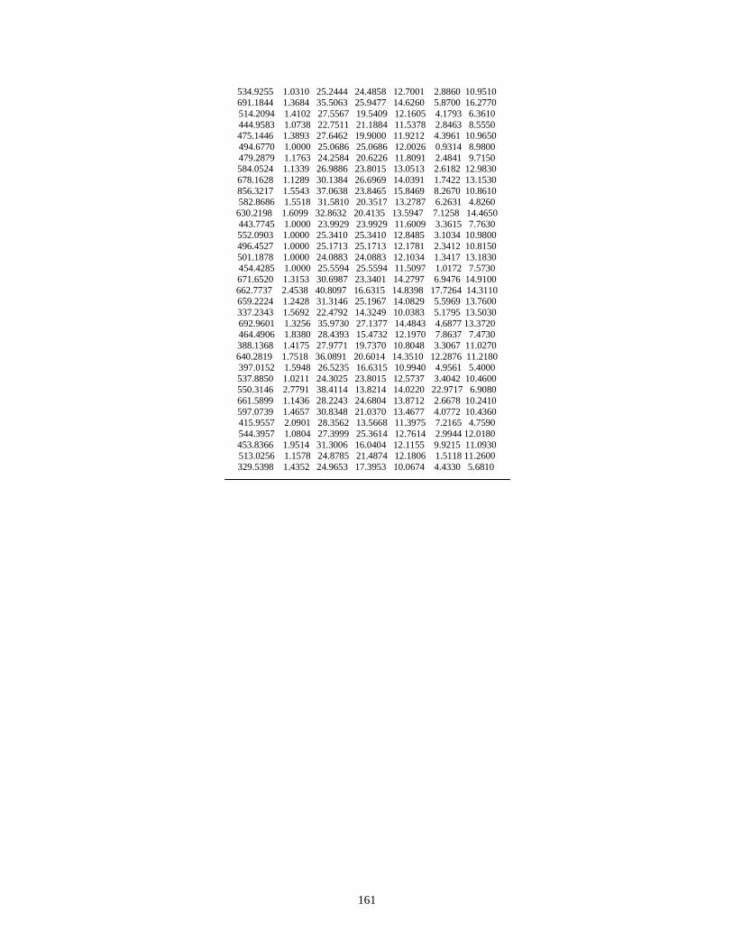
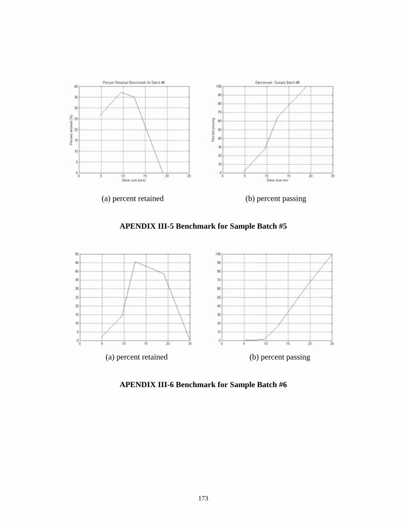
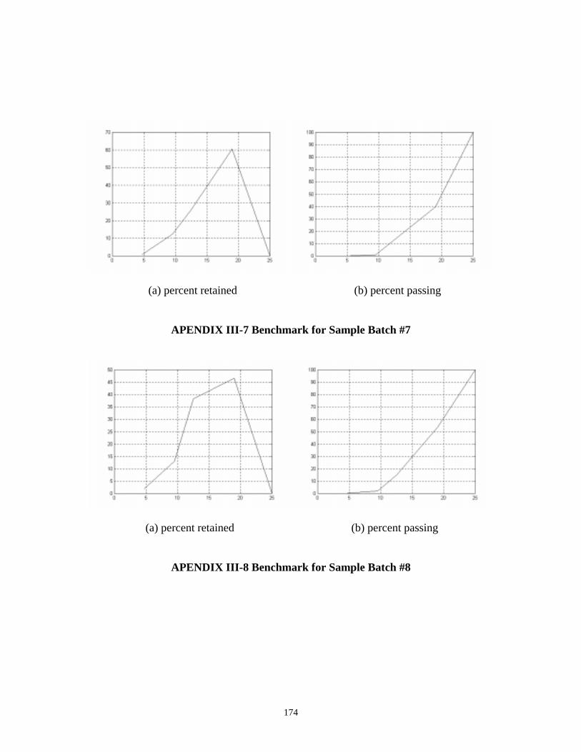
Table 8.1 : Statistics of the Benchmark (Sieving of 10 times) ……………………….142
Table 8.2 : Percent Retained Result Comparison ……………………………...……..143
Table 8.3 : Percent Passing Result Comparison …….………………………………..144
1
1. INTRODUCTION
1.1 Historical Background
Hot-mix asphalt concrete is widely used to build modern highways. The strength
and durability of asphalt concrete pavements are profoundly affected by the
characteristics of the aggregates. Beyond the obvious dependence on aggregate’s
properties such as the strength and durability, characteristics such as particle shape, and
gradation (i.e., size distribution) are extremely important. Research performed as part of
the Strategic Highway Research Program provided a standard for asphalt concrete mix
design called “Superpave” [1], which specifies limits for aggregate gradation, particle
angularity, and percentage of thin and elongated particles.
The particle size distribution in the mixed asphalt plays a vitally important role in
the quality control for the highway building. For instance, pavements constructed with
too high a percentage of fine particles such as natural sand will display unallowable
levels of permanent deformation when loaded by traffic. On the other hand, too many
large particles in the mixed asphalt can produce a large amount of voids. As a result, the
strength and durability of the pavement will be compromised. The quality of pavement
demands the appropriate mixture of various sizes of particles, and the size distribution of
the mixture is presented by the gradation curve.
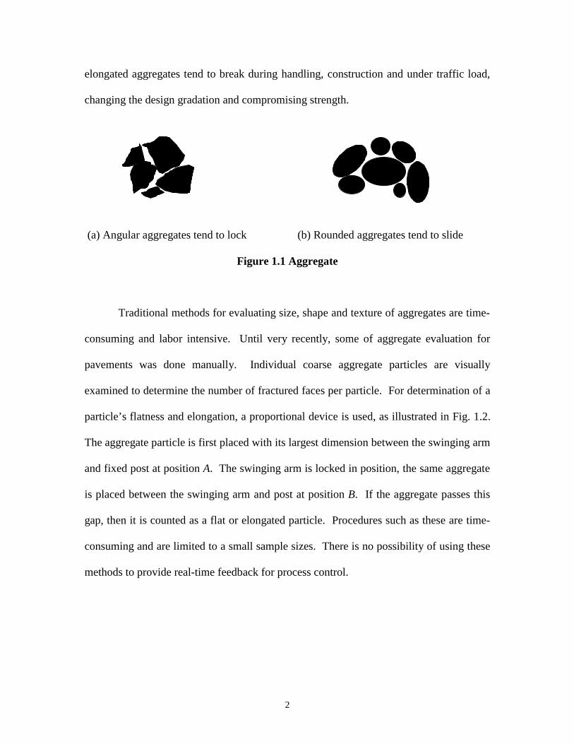
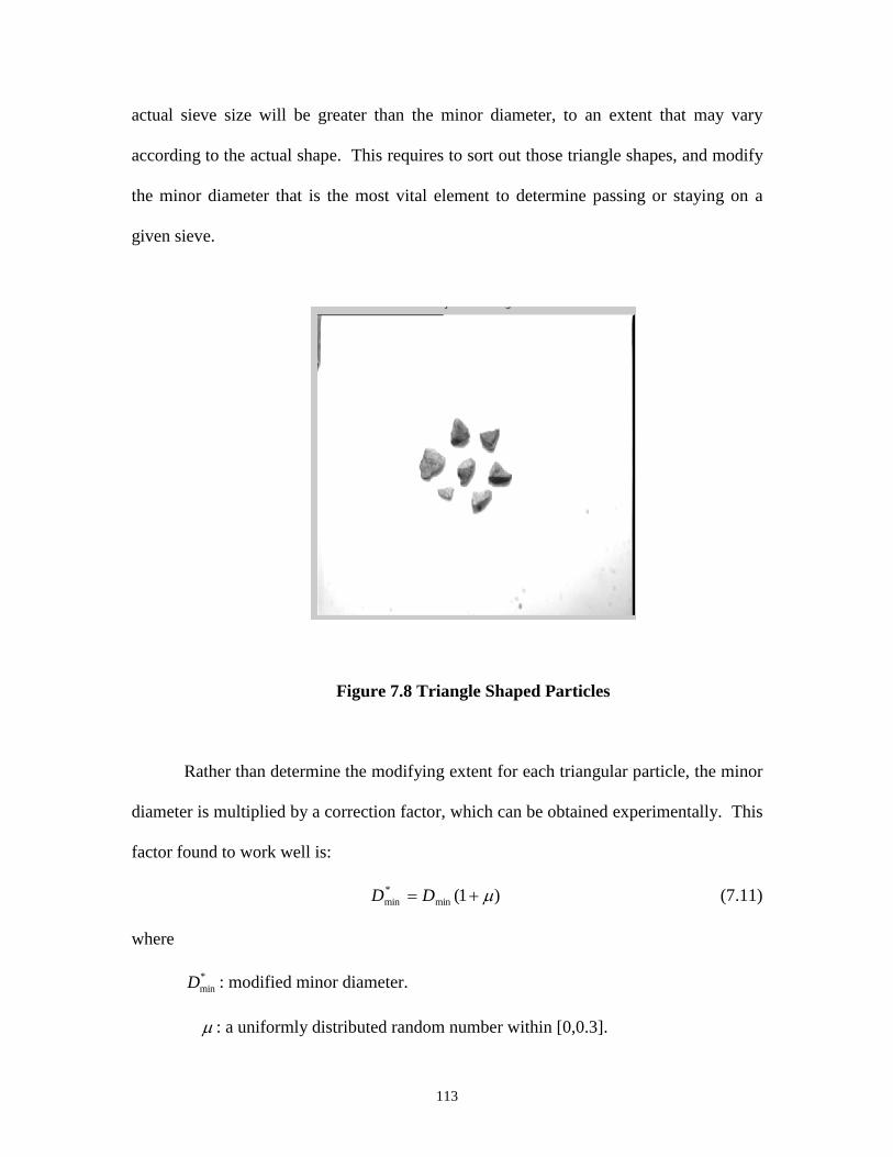
Particle shape is also important because rough or angular aggregates provide more
strength than rounded, smooth-textured aggregates as shown in Fig. 1.1. Even though a
jagged piece and a rounded piece of aggregate may possess the same material strength,
angular aggregate particles tend to lock together resulting in a stronger mass of material.
On the other hand, rounded aggregate particles tend to slide by each other. Flat and
2
elongated aggregates tend to break during handling, construction and under traffic load,
changing the design gradation and compromising strength.
(a) Angular aggregates tend to lock (b) Rounded aggregates tend to slide
Figure 1.1 Aggregate
Traditional methods for evaluating size, shape and texture of aggregates are time-
consuming and labor intensive. Until very recently, some of aggregate evaluation for
pavements was done manually. Individual coarse aggregate particles are visually
examined to determine the number of fractured faces per particle. For determination of a
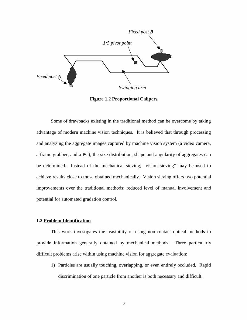
particle’s flatness and elongation, a proportional device is used, as illustrated in Fig. 1.2.
The aggregate particle is first placed with its largest dimension between the swinging arm
and fixed post at position A. The swinging arm is locked in position, the same aggregate
is placed between the swinging arm and post at position B. If the aggregate passes this
gap, then it is counted as a flat or elongated particle. Procedures such as these are time-
consuming and are limited to a small sample sizes. There is no possibility of using these
methods to provide real-time feedback for process control.
3
Fixed post B
1:5 pivot point
Fixed post A
Swinging arm
Figure 1.2 Proportional Calipers
Some of drawbacks existing in the traditional method can be overcome by taking
advantage of modern machine vision techniques. It is believed that through processing
and analyzing the aggregate images captured by machine vision system (a video camera,
a frame grabber, and a PC), the size distribution, shape and angularity of aggregates can
be determined. Instead of the mechanical sieving, “vision sieving” may be used to
achieve results close to those obtained mechanically. Vision sieving offers two potential
improvements over the traditional methods: reduced level of manual involvement and
potential for automated gradation control.
1.2 Problem Identification
This work investigates the feasibility of using non-contact optical methods to
provide information generally obtained by mechanical methods. Three particularly
difficult problems arise within using machine vision for aggregate evaluation:
1) Particles are usually touching, overlapping, or even entirely occluded. Rapid
discrimination of one particle from another is both necessary and difficult.
4
2) Standards for classifying particles by size are generally based on mechanical
sieving and the process results depend on a combination of both size and 3-
dimensional shape of particles. It is desirable to avoid the complexity and
expense of explicitly measuring the 3rd dimension of each particle.
3) Sieving standards are also set up to report particle gradation on a “percent
passing” basis, where the fraction is based on mass. So in addition to
extrapolation of the interaction between a particle’s 2-D features and the
sieving process, it is necessary to develop a means to extrapolate the
relationship between a particle’s 2-D features and its volume. These
extrapolations will be dependent on general size and shape properties that
vary from particle to particle. For example spherical particles will have
different sieving and volume transformation than cylindrical, cubic, or
triangular particles.
The fundamental question is then, “Can we extract a set of features from the 2-D
image which will provide adequate information to accurately predict volume
characteristics, elongation, angularity, and the sieving behavior from the particles’ 2-D
video image?”
1.3 Research Objectives
The work can be broken into three major tasks as follows:
1) To effectively describe the sieving characteristics of 3-D aggregates based on
2-D geometric size and shape of the particles.
5
2) To develop a functional relationship between a particle’s plan features and its
corresponding volume. In other words, inferring volume information of the 3-
D particle under consideration by means of measurements obtained from 2-D
image. This will be the main theme of this research.
3) To develop a simple and efficient method that can separate the touching and
overlapping particles in the scene.
1.4 What is Superpave?
From 1987 through 1992, the Strategic Highway Research Program (SHRP)
conducted a research effort to develop new ways to specify, test, and design asphalt
materials. After 1992, the Federal Highway Administration (FHWA) assumed a
leadership role in the implementation of SHRP research. An essential part of FHWA’s
implementation strategy was educating agency and industry personnel in the proper use
and application of the final SHRP asphalt products, collectively referred to as Superpave
[1].
Definitions for properties of aggregate such as size, shape and texture may vary
from standard to standard, depending on the agencies involved. However, because this
research is a project aimed at improving methods of aggregate gradation and shape
identification, size, shape and other related definitions given in the Superpave guide book
have become the guidelines in terms of comprehending the aggregate’s characteristics.
6
1.4.1 Aggregate Size
Many technical reports in the field of mineral aggregate property studies
explicitly or implicitly regard the area of the particle in a 2-D plane as particle size [3, 4,
5, 6]. In Superpave [1], the aggregate size is considered as being the dimension of a
square sieve opening through which the particle falls by its own gravity. Let a sieve size
be a square of Di�Di, where Di takes a discrete value of a sequence with DN>DN-1>DN-
2…>D1. The aggregate size d is then a value that satisfies
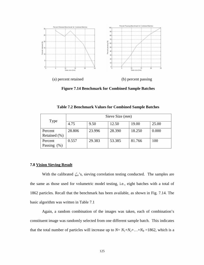
Di-1< d � Di (1.1)
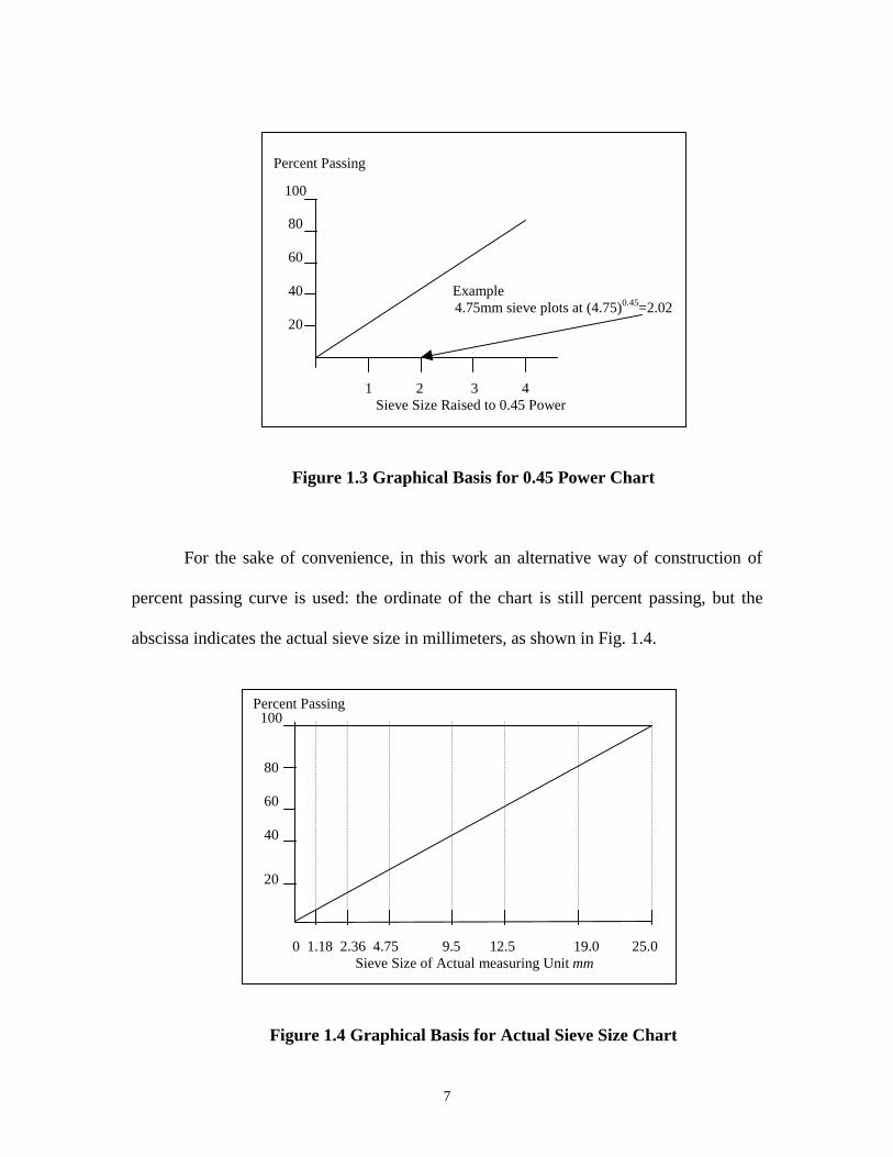
Superpave prefers to use the 0.45 power gradation chart to define an allowable
gradation limits. This chart uses a unique graphing technique to judge the cumulative
particle size distribution of a blend of aggregates. The ordinate of the chart is percent
passing, the abscissa is an arithmetic scale of sieve size in millimeters, raised to 0.45
power. Fig. 1.3 illustrates how the abscissa is scaled. In this example, the 4.75 mm sieve
is plotted as 2.02 units to the right of the origin.
7
Figure 1.3 Graphical Basis for 0.45 Power Chart
For the sake of convenience, in this work an alternative way of construction of
percent passing curve is used: the ordinate of the chart is still percent passing, but the
abscissa indicates the actual sieve size in millimeters, as shown in Fig. 1.4.
Figure 1.4 Graphical Basis for Actual Sieve Size Chart
Percent Passing
100
80
60
40 Example 4.75mm sieve plots at (4.75)0.45=2.02
20
1 2 3 4 Sieve Size Raised to 0.45 Power
Percent Passing 100
80
60
40
20
0 1.18 2.36 4.75 9.5 12.5 19.0 25.0 Sieve Size of Actual measuring Unit mm
8
1.4.2 Aggregate Shape
The Superpave manual [1] describes the particle shape as:
� Flat and elongated: The ratio of a maximum to minimum dimension is greater
than 5.
The aspect ratio of the particle can be used for detection of elongated shape.
Aspect ratio is defined as the ratio of the maximum diameter to the orthogonal minimum
diameter of the shape silhouette.
In Superpave, shape identification is performed by obtaining the percentage by
mass of coarse aggregates that are elongated. Elongated particles are undesirable because
they have a tendency to break during construction and under traffic.
9
2. LITERATURE REVIEW
2.1 Introduction
This research is associated with many aspects in the fields of image processing,
image analysis and statistics. Related work in image processing mainly involves image
segmentation, more specifically, separation of touching and overlapping shapes, and
object size and shape characterization. To optically “sieve” the particles, it needs to
predict the particle mass based on 2-D image measurements.
There are many publications on image edge detection, image size and shape
analysis. Many techniques in shape characterization such as Fourier analysis and
template matching have been reported in literature. Some novel methods such as
polygonal harmonics are also attracting attention. By comparison, fewer articles
regarding separation of the touching and overlapping imaged shapes exist. There are
some reports about inferring the objects’ 3-D information (volume) from their 2-D
measurements. Some insights into optical sieving may be shared from the reports on
existing technology, and several video graders using these technologies have been
marketed commercially.
2.2 Existing Technology
In searching for the work related to this research project, only three commercial
products that perform the functions desired for Superpave quality control were
discovered. There are some helpful descriptions of these three commercially available
systems given by H. Kim, et al [33].
10
The EMACO corporation of Montreal, Canada markets a device called the VDG
40TM, which uses optical methods to perform particle sieving. The VDG 40 employs a
line-scan camera and approximates particle boundaries by drawing successive chords
across the particles falling off the vibrating feeder. Although there has been some debate
about its accuracy by some independent testers [32], this system is claimed to perform the
following functions:
� Produce gradation curves for particles whose sizes range from 1 to 50 mm.
� Calculate mean elongation coefficient.
� Estimate the “flattening coefficient”.
� Uncertainty less than 1.7% for samples with enough particles in each class.
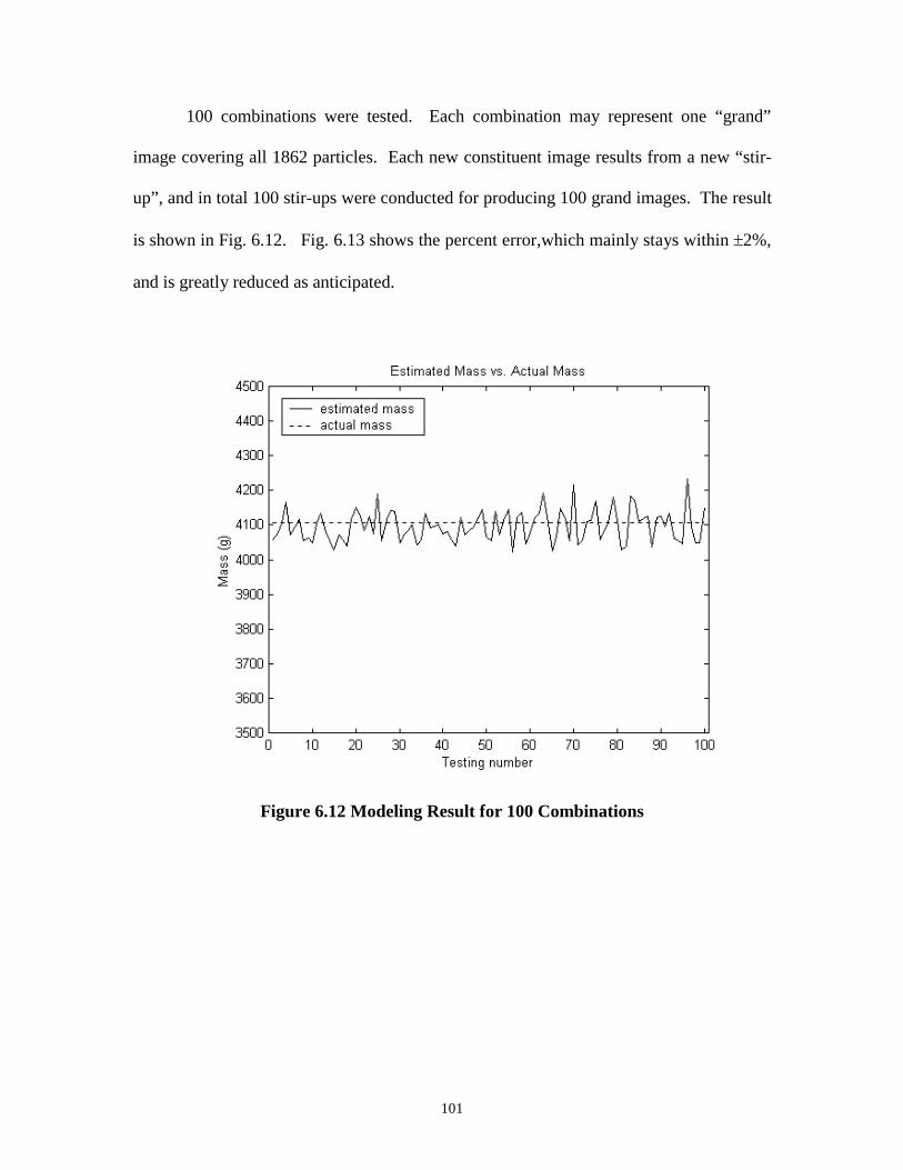
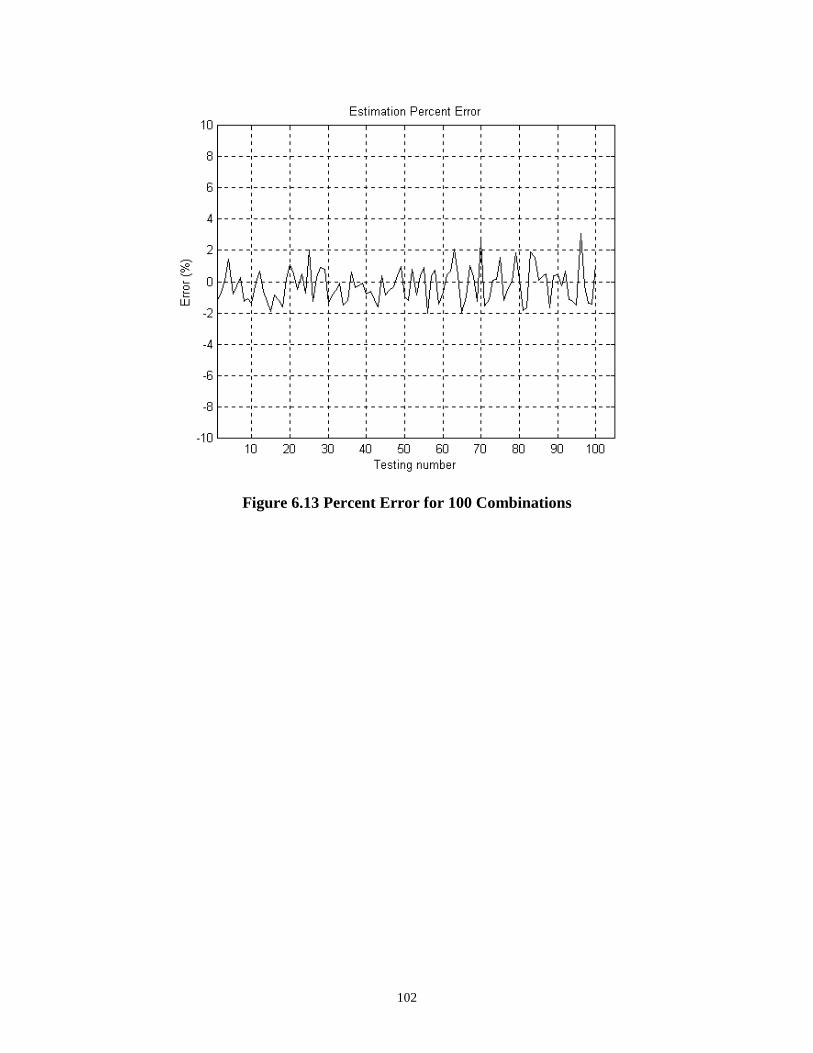
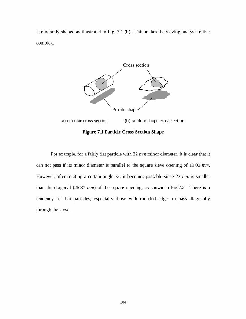
Based upon the assumption that the thickness of the particle is the same as its
width, the volume is computed using an ellipsoid of revolution [32]. No clear
information about how to separate the touching and overlapping is provided even though
the falling particles may be overlapped when viewed in any direction. A description of
the on-going effort on testing and improving VDG 40 is summarized by R.L. Weingart,
et al [31].
Several products are marketed by the WipWare Company in Bonfield, Ontario,
Canada [35, 39]. WipFragTM performs optical gradation on bulk materials on the ground
or on moving conveyor belts. The WipFrag system is based on area scan video cameras.
Some case studies using the Wipfrag image analysis system were presented by Maerz
[40]. Another product, WipShape, uses a conveyor and two video cameras to image one
particle at a time and compute the percentage of flat, elongated particles [35, 37].
11
N.H. Maerz used stereology and object geometric probability to explore the
possible solution of the problem of inferring the true size distribution of a body of
particles, given the observed profile distribution on an imaged scene [27]. The process is
known in stereology as “unfolding” a distribution. The problem is: can one reconstruct a
block size distribution of a pile of blast fragmented rock from a measurement made on
the surface of that pile? Maerz found that if one applies the stereological theory
developed by previous researchers to this problem, many of the assumptions made for the
existing theory are violated. Therefore, Maerz suggested a new method of unfolding the
distribution.
This new method is based on analyzing fragmentation using image analysis, and
first assuming all particles to be spherical for a quick solution. The distribution from the
image can be calculated. Maerz states that the observed distribution should be further
divided into a number of classes, in each of which the particles have a similar diameter. A
calibration function was added to account for numerous effects to improve algorithm’s
accuracy. This makes the equation become “semi-empirical”. The calibration function is
determined by back calculation from a known size distribution.
An experimental system is under development by Rao, et al at the University of
Illinois [32]. Rao developed an experimental device that uses three cameras to capture
orthogonal images of a single particle at a time. Rao’s objective is to improve the
detection of flat, elongated particles, and it was claimed that the system performs more
accurately than either the VDG 40 or the WipFrag system [32]. The tests have
demonstrated volume measurement errors ranging from 5% to more than 10%, but errors
in detection of flat, elongated particles were within approximately 1-2%. Rao’s device is
12
quite slow, however. A processing time for 1037 particles of 70 minutes was reported.
The volume errors are also relatively high (�10%) when compared with the published
claims of commercially available systems [31].
The method of calculating aggregate volume is straight forward. Three video
cameras are mounted from three orthogonal directions: front, side, and top. The images
acquired from these three views provide some capability to reconstruct the 3-D shape of
the particle needed for volume computation. The particle is confined in the smallest box
whose sides are found to be the smallest rectangle that includes the particle projected area
in that viewing direction. Those pixels, called solid pixels, can be found readily which
belong to the particle body from all three viewing directions. All the cubes made up of
the solid pixel are summed up, and calibrated to cubic millimeters. Hence, the volume of
the particle under study is obtained. However, it is fairly easy to envision shapes for
which even three orthogonal views are taken would not be sufficient to accurately
evaluate particle volume [33]. The particle touching and overlapping problem is avoided
because all particles fall one at a time onto a belt that is in motion. Though the system
performance is expected to give improved accuracy, it is more time consuming since the
particle is processed individually on a conveying belt.
The Micrometrics Corporation sells a device similar in design to the VDG 40.
The Optisizer PSDATM uses a vibrating feeder and a CCD camera to capture a 2-D image
of particles from 40 micrometers to “greater than 10 mm” [36]. This device is more suited
to pharmaceutical environments than construction work, however. No mention of particle
shape analysis is provided, nor are statistics on the sieving accuracy of the machine.
13
In addition to these devices, articles related to optical sieving or particle size and
shape evaluation have been published in the technical literature by a variety of authors.
Parkin, et al published a proposal for a laser based aggregate scanning device in 1995, but
no further references to their system have been found [4].
2.3 Separation of Overlapping Image Objects
Bennamoun and Bouashash [3] introduced a segmentation method based on the
successful completion of robust edge detection. The segmentation algorithm begins with
extracting the convex dominant points (CDP), then use these CDP’s for the part
segmentation by simultaneously moving each of them normal to the edge contour until
one CDP touches another point. Next the initial locations of CDP’s are joined to the
touched points. This process is repeated until the whole object has been segmented into
constituent parts. The segmented parts are then isolated and modeled by superquadratics
with varying parameters for recognition purposes.
A templating approach for separating the touching and overlapping spots is
introduced by Noordmans and Smeulders [14]. The technique consists of two phases:
detection phase and characterization phase. In the detection phase, all image positions
are matched to a spot model with predefined parameter vector and coordinate. The
optimal match is given by the specific value of parameter vector that results in a minimal
match error. Following the detection phase is the characterization phase. The primary
purpose of this phase is to further reduce the match error. Detecting two overlapping
spots is based first on the observation of two major match errors, then extracting the local
image. After removing one neighboring spot, the first spot is optimally matched with the
14
model using numerical minimization procedure. By the same method, the second spot can
be detected and characterized. This way, two overlapping spots are thus detected and
characterized independently.
In morphological image processing, the watershed detection approach proves to
be an efficient way of segmenting gray scale images or binary images. Vincent [28]
provides a faster, more efficient algorithm than those introduced previously to detect the
watershed for a gray toned image. The basic principle behind this technique is that the
whole gray scale image under study is considered as a topographic surface. This surface
is made up of basins (valleys) and mountains. The watershed algorithm computes the
dividing lines between the different “catchment basins”, which become regions or objects
in the image. In the case of a binary image, the effect is to separate touching or
overlapping particles. A modification of this approach was developed for use in this
research.
2.4 Particle Passage Probability in Sieving
Most probabilistic studies of particle-passage through a sieve relate the
probability of passage to sieve aperture size and particle shape. Bocoum [41] reviewed
some probability theory in sieving. In summary, the particle-passing probability through
a screen depends on the following aspects:
1) Three dimensional shape of the screen, and
2) Its relative size to the size of the particle
3) The percentage of open area on the screen surface.
4) Screen surface roughness.
15
5) The speed of the particle upon impact.
The primary studies of particle-passing probability were developed for particles of
three geometric shapes: spheres, ellipsoids, and cylinders. For these three shapes, the
theoretic passing probability was reviewed in Bocoum’s paper. However, no conclusive
information was presented for the irregularly shaped particles passing through the square
sieve aperture.
2.5 Object Shape
Particle shape is an important factor in particle handling and product quality
control. Since the particle shape influences how particles flow, react, sinter, break,
agglomerate, and fluidize, numerous shape characterization techniques have been
demonstrated over the last decades [8].
Particle shape analysis can be divided into two broad categories: behavior
analysis and image analysis [9]. Most image analysis techniques rely on examining a
two-dimensional image silhouette of the particle shape. Analysis of particle image can be
conducted in either a microscopic or macrosopic manner. The microscopic method is
used to describe the particle’s relatively subtle change on the surface such as angularity
and roughness. The macroscopic method, on the other hand, is more general in the sense
of describing particle shape. This approach usually provides information in 2-D image
about particle characterized shape such as triangle, four-sided, etc.
In a microscopic shape study, Clark made some explorations of fractal analysis
[7]. Fractal analysis originates from the fact that the perimeter of the silhouette edge is
dependent on the step length with which it is measured. The small detailed features on
16
edge can be taken into account with step length small enough, while taking large step
length will ignore some delicate characteristics of the edge. The measured perimeter is
increased if the step length used is decreased, yielding the notion of “fractal dimension”
that can be used to describe particle ruggedness over a range of scale. A logarithmic plot
of perimeter against step length produces a curve with negative slope. Steepness of the
curve slope is used as a descriptor indicating the extent of the ruggedness of that particle
silhouette. Fractal dimension shows the general degree of particle ruggedness, but does
not provide general geometric shape information.
In a more macroscopic approach, Clark, and Reilly introduced a novel approach
called polygonal harmonics to describe the particle shape [9, 10]. A starting point is
selected on the edge of the particle, then a pair of dividers is set at some distance and
used to find another point on the curve. Sequential points on the edge are found in the
same manner by marching along the edge of the particle. The procedure is similar in
this regard to a structured walk to find fractal dimension as mentioned previously. The
walk continues past the first starting point, traversing the silhouette edge over and over
again. Eventually a polygon is formed with a fixed dividing step length within the
shape. Different step lengths produce different polygons for the same particle shape.
Harmonic persistence is defined as the ratio of the largest step length to the smallest
step length yielding that particular polygon. High harmonic persistence is an indicator
of general particle shape.
This approach has shown some satisfactory results. However, in general it does
not guarantee that a particular polygon exists for a given shape silhouette. Repetition of
computation using different step lengths to find harmonics persistence is needed for each
17
particle [10]. Moreover, the persistences are not unique to each analytical shape, nor can
the shape be reconstructed using the persistences [12].
Fitting approaches have been found in a variety of literature. In the papers by
Bennamoun and Bosshash [3], Rosin and West [6], object shapes are described by fitting
the object edge silhouette with superellipses. Each superellipse is described by three
parameters: major and minor axis, and shape factor. One superellipse can be found to be
the best fit to the shape in question by minimizing the Eucidean distance between the
point on the superellipse and the point on the edge silhouette. Using the three identified
parameters of this particular superellipse, the shape can thus described. The advantage of
this technique is that a superellipse can represent a wide variety of shapes. with a small
number of parameters.
Another template matching is to fit the object edge silhouette with a square
instead of a superellipse. The side length of the square is used as the descriptor for the
shape to show how square-like or rhombic-like that particle is. The best fitting square
is found by minimizing the area error between the square and the particle of interest.
The merit of this technique is that only a few parameters are necessary for describing
the shape in question. However, neither the superellipse nor the square fitting approach
can accurately represent shapes with odd numbers of sides. For instance, a triangle
shaped particle can never be fitted well by either the superellipse or square. Moreover,
both techniques are computationally intensive. Algorithm convergence is not always
guaranteed. This disadvantage is even more severe when applied to a large number of
particles in a single image.
18
A set of descriptors called “invariant moments” was studied [2]. Invariant
moments are derived using the central moments of the image shape. Because of the
relation of central moments with the regular moments, and the uniqueness of these
regular moments relating to a certain image function, the chance that different shapes
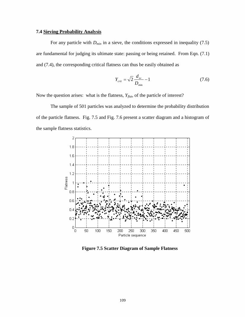
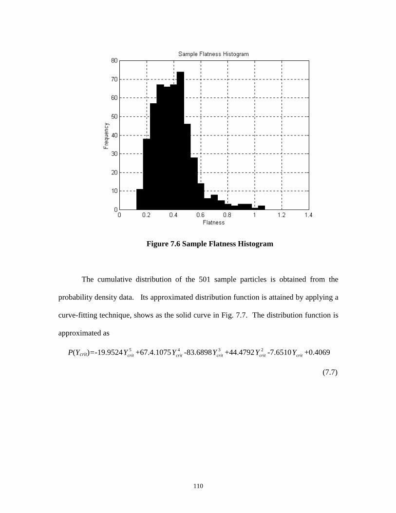
have the same or even close invariant moments is small. Therefore, invariant moments
can be utilized to describe the shape features.
All the above shape descriptors share the same merit: they are translation-
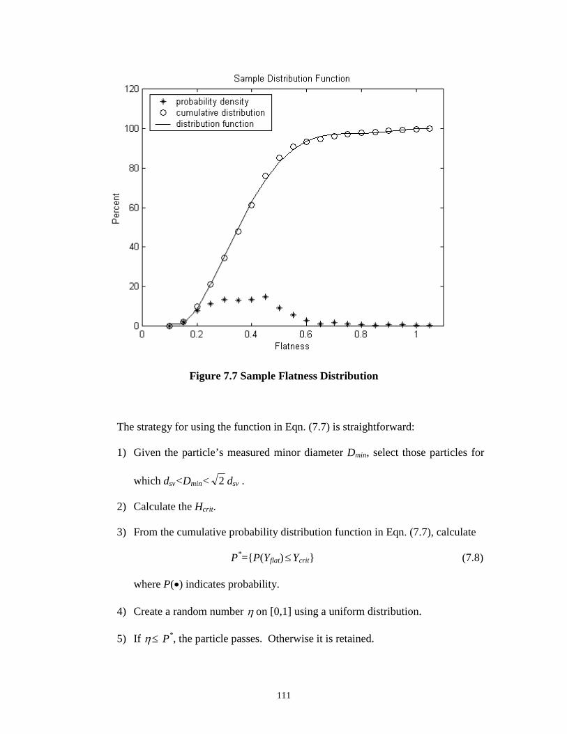
invariant, rotation-invariant, and scale change invariant. These attributes are necessary
for shape feature classification in a multi-object situation. The negative aspect about
using the above techniques is the computational intensity.
Fourier analysis has long successfully employed on smooth, rounded particles. In
Fourier analysis, the edge is described by expressing the radius from the centroid of the
shape as a function of the swept angle, using a Fourier series. For instance, the second
coefficient gives an implication of aspect ratio, and the third coefficient indicates
triangularity, and so on. Particle shapes can be compared in a n-dimensional space
composed of the n orthogonal Fourier coefficients [13]. The well-known weakness of
Fourier analysis lies in the fact that it does not deal efficiently with highly reentrant
shapes.
2.6 Object Size
Size and shape issues are usually intertwined in image processing problems.
Various specifications for object size description have been found in technical reports: for
objects of regular shapes such as squares and circles, side length and diameter are used
19
respectively to define sizes. For irregularly shaped objects, major and minor dimensions
are well-defined measures, although they do not guarantee uniqueness of shape
description. Size, defined by the object’s projected area, can be found explicitly and
implicitly described in various papers. In Rosin and West [6], it can be inferred that the
size is defined by the parameters of the superellipses, and is also represented by its area.
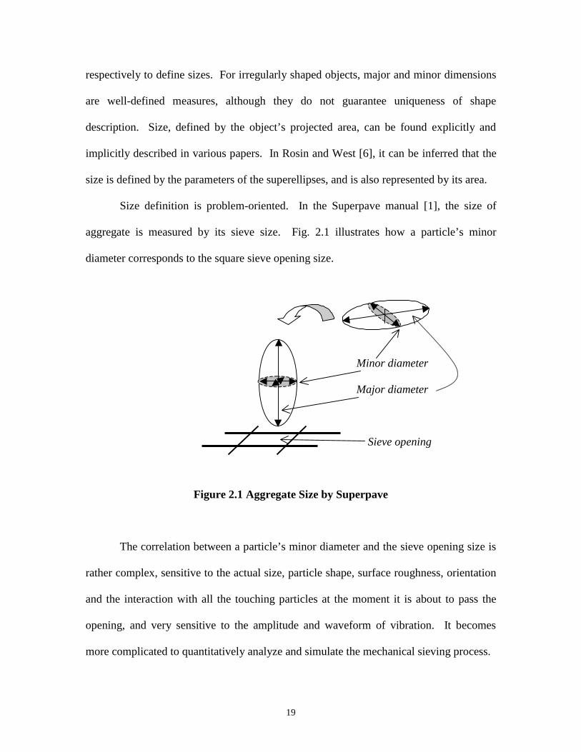
Size definition is problem-oriented. In the Superpave manual [1], the size of
aggregate is measured by its sieve size. Fig. 2.1 illustrates how a particle’s minor
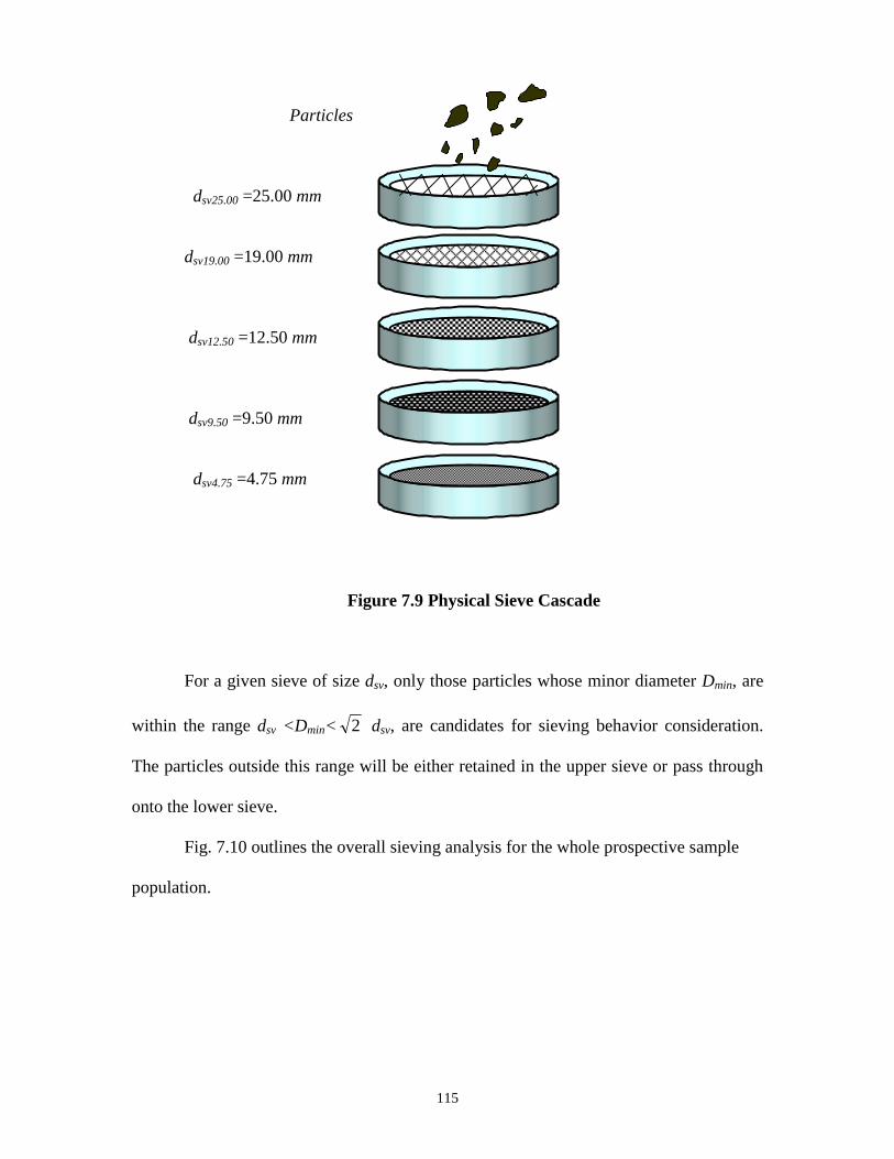
diameter corresponds to the square sieve opening size.
Minor diameter
Major diameter
Sieve opening
Figure 2.1 Aggregate Size by Superpave
The correlation between a particle’s minor diameter and the sieve opening size is
rather complex, sensitive to the actual size, particle shape, surface roughness, orientation
and the interaction with all the touching particles at the moment it is about to pass the
opening, and very sensitive to the amplitude and waveform of vibration. It becomes
more complicated to quantitatively analyze and simulate the mechanical sieving process.
20
3. LABORATORY SET-UP AND
MEASUREMENT CALIBRATION
3.1 Introduction
A video camera translates light levels focused on the image plane into electronic
signals which can be transmitted and reproduced on a monitor set. The most common
type of video camera uses a charge coupled device (CCD) chip to translate the light into
electrical signals. The CCD chip is actually a grid of tiny individual light measuring
devices which break the scene up into individual picture elements, or pixels. The camera
used for this research breaks each scene into an array of 512 pixels wide and 484 pixels
high.
To process these signals using a computer, the light level represented by the video
signal must be digitized by translating the signals into a series of numbers that the
computer can manipulate. This is implemented by a frame grabber board, which
performs very fast analog-to-digital conversion on the electronic signal for the camera.
As a result, a grid (matrix) of numbers ranging from 0 to 255, with one number for each
pixel, is formed. Low numbers represent dark parts of the image and high numbers
represent bright parts of the image.
To optically sieve the particles, it is necessary to translate the pixel measurements
into standard dimensions of millimeters. Pixels are in general not square, and so a unit of
one pixel represents a different length in the x direction than it does in the y direction. In
addition, the object is projected optically onto a CCD array. This causes the size of the
image to depend not only on the size of the object but also on its distance from the
camera, and on the focal length of the lens used to project the image onto the CCD
21
sensor. Therefore, a scale of mm / pixel needs to be determined before any useful image
analysis takes place.
3.2 Hardware Set-up and Operating Condition
The laboratory consists of a video camera housed in a curtained enclosure to
allow control of the lighting conditions, a computer with a frame grabber card, a box with
translucent cover to backlight the aggregates, and miscellaneous equipment for scene
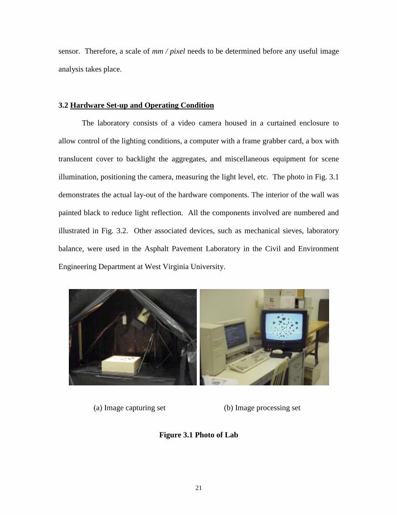
illumination, positioning the camera, measuring the light level, etc. The photo in Fig. 3.1
demonstrates the actual lay-out of the hardware components. The interior of the wall was
painted black to reduce light reflection. All the components involved are numbered and
illustrated in Fig. 3.2. Other associated devices, such as mechanical sieves, laboratory
balance, were used in the Asphalt Pavement Laboratory in the Civil and Environment
Engineering Department at West Virginia University.
(a) Image capturing set (b) Image processing set
Figure 3.1 Photo of Lab
22
(6) ` (7)
(2) (3)
(8) (9) (4) (5)
(1)
3.2 Lab Equipment Lay-out
Referring to Fig. 3.2, the representation of the numbered item is as follows:
(1) Stationary table.
(2) Pan-tilt device with 6-degrees of freedom.
(3) Video camera.
(4) High contrast lighting box.
(5) Aggregate particles.
(6) Photographic strobe light for oblique lighting.
23
(7) Personal computer with frame grabber.
(8) Light intensity meter.
(9) Monitor.
The operating specifications for image capturing using the lighting box are given
in the table below:
Table 3.1 Operating Condition
CameraDistance frombackground
20 inches Cameraaperture 6
CameraFocus
20 inchesAmbient lightingintensity
12 LUX
CameraShutter speed
1/125 Sec
3.3 Image Acquisition
In order to properly “sieve” the aggregates, it is necessary to distinguish one
particle from another in the video image. The gray scale video images that are most
commonly seen, seem simple to the human observer to see where object boundaries are,
while the information presented to the computer from these images is nothing more than
a large grid of numbers. To detect these boundaries, most approaches involve some sort
of gradient detection - looking for places in the image where there are rapid changes
from light to dark or vice versa. Some of the object boundaries are clearly defined by
contrast between the background and the existence of object shadows. But if imaged
objects such as mineral particles overlap, the contrast between two particles may not be
so distinct. In addition, the existence of ridges or corners on the particles can produce
high-contrast edges which are not true particle boundaries in the 2-D sense.
24
Various edge-finding algorithms and lighting angles were explored to find a
method that would reliably detect the boundary of each particle. The simplest and most
common edge detectors are first-order high-pass filters based on the Sobel Operator or
variants thereof [2]. These filters are highly sensitive to noise and directional in nature,
performing best on edges that are either vertical or horizontal. Sobel filters combined
with top lighting are also prone to including unwanted edges, such as those resulting from
corners or shadows on the top surface of the particle.
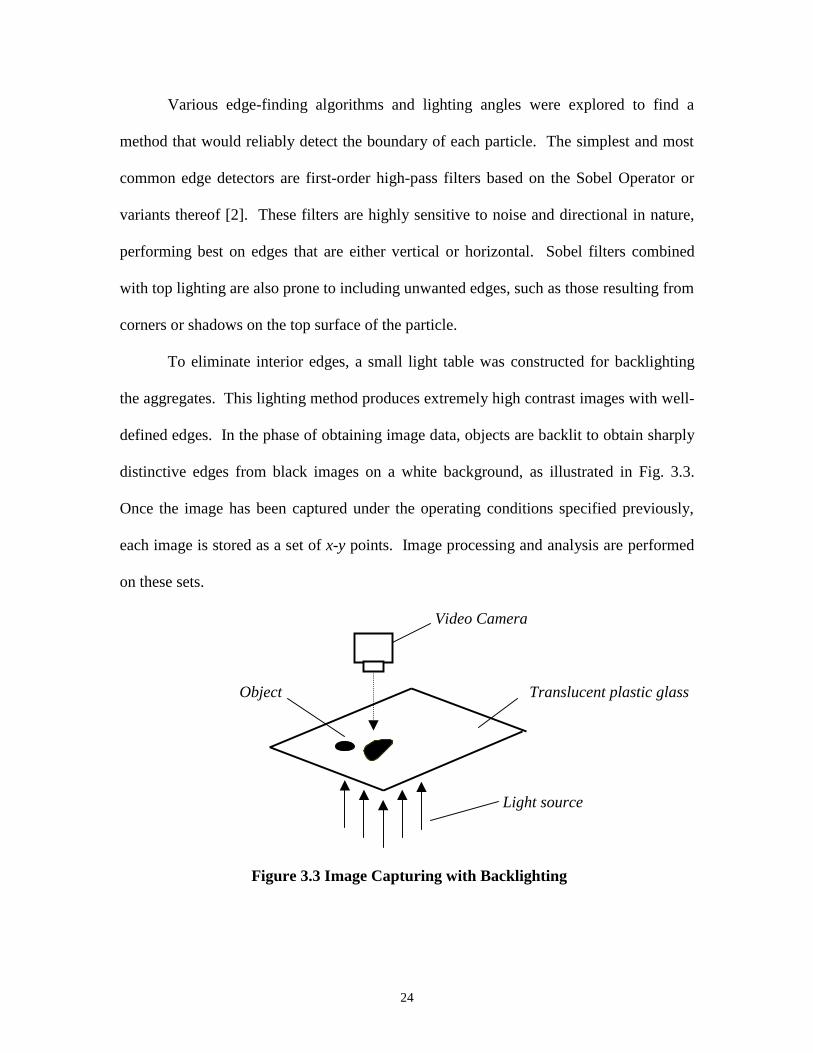
To eliminate interior edges, a small light table was constructed for backlighting
the aggregates. This lighting method produces extremely high contrast images with well-
defined edges. In the phase of obtaining image data, objects are backlit to obtain sharply
distinctive edges from black images on a white background, as illustrated in Fig. 3.3.
Once the image has been captured under the operating conditions specified previously,
each image is stored as a set of x-y points. Image processing and analysis are performed
on these sets.
Video Camera
Object Translucent plastic glass
Light source
Figure 3.3 Image Capturing with Backlighting
25
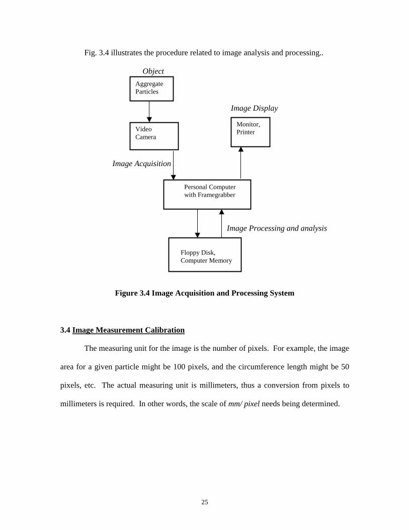
Fig. 3.4 illustrates the procedure related to image analysis and processing..
Object
Image Display
Image Acquisition
Image Processing and analysis
Figure 3.4 Image Acquisition and Processing System
3.4 Image Measurement Calibration
The measuring unit for the image is the number of pixels. For example, the image
area for a given particle might be 100 pixels, and the circumference length might be 50
pixels, etc. The actual measuring unit is millimeters, thus a conversion from pixels to
millimeters is required. In other words, the scale of mm/ pixel needs being determined.
VideoCamera
Monitor,Printer
Personal Computer with Framegrabber
Floppy Disk, Computer Memory
AggregateParticles
26
3.4.1 Sample for Calibration
Three types of sample circles were found using penny, nickel, and quarter. Their
diameters are 19.05mm, 21.12 mm, 24.20 mm, respectively. The corresponding areas
are 285.02 mm2, 350.33 mm2, and 459.96 mm2. The distance between the camera and
the imaging background is 20 inches, set constant for all images. The parameters of the
camera such as shutter speed and aperture were unchanged during the imaging process.
Fig. 3.5 shows the samples used for calibration.
(a) Pennies (b) Nickels (c) Quarters
Figure 3.5 Samples for Calibration
3.4.2 Finding Pixel Number
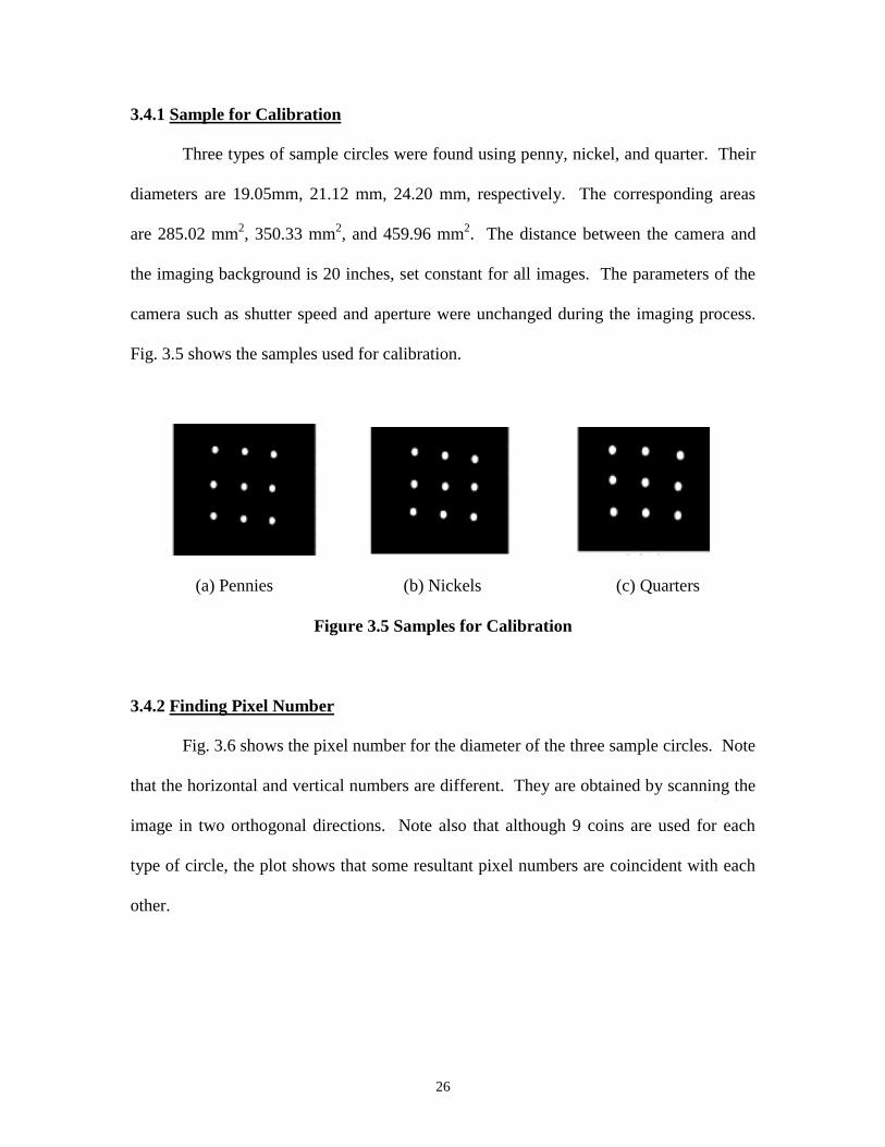
Fig. 3.6 shows the pixel number for the diameter of the three sample circles. Note
that the horizontal and vertical numbers are different. They are obtained by scanning the
image in two orthogonal directions. Note also that although 9 coins are used for each
type of circle, the plot shows that some resultant pixel numbers are coincident with each
other.
27
Figure 3.6 Maximum Pixel Number
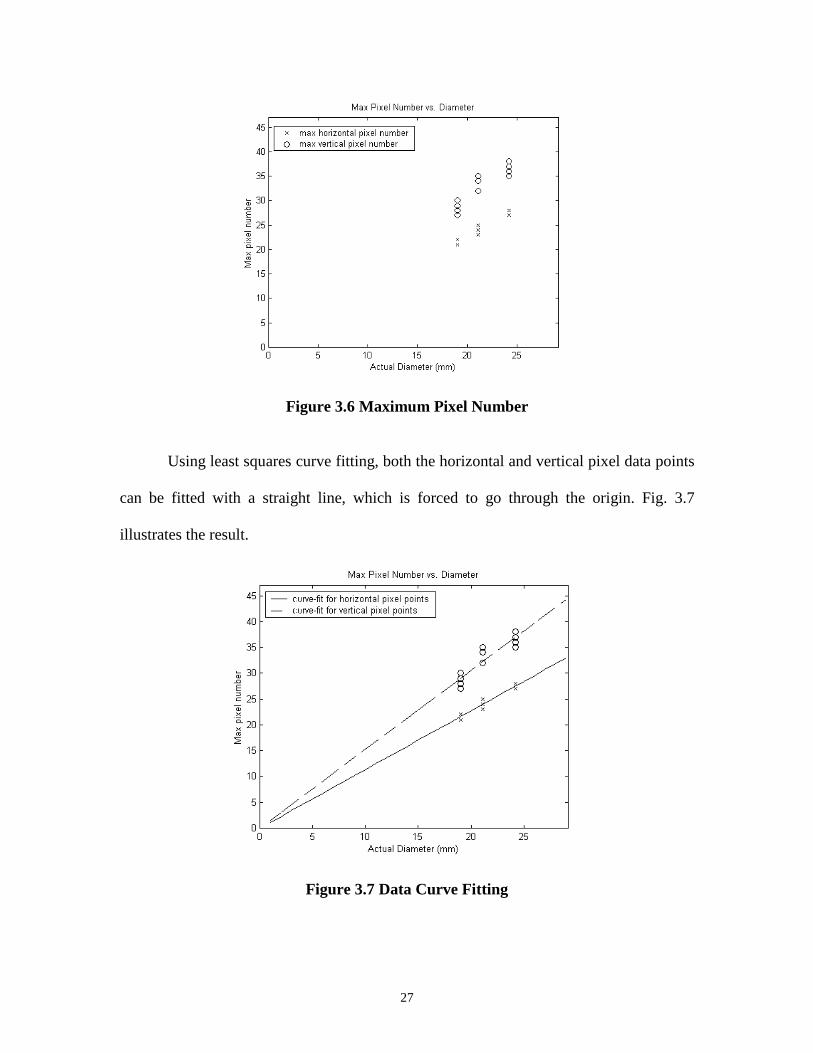
Using least squares curve fitting, both the horizontal and vertical pixel data points
can be fitted with a straight line, which is forced to go through the origin. Fig. 3.7
illustrates the result.
Figure 3.7 Data Curve Fitting
28
The reciprocal of the slope of each straight line is taken as the desired scaling
factor of mm / pixel . The results are: 0.8802 mm/pixel in the horizontal direction, and
0.6551 mm/pixel in the vertical direction.
3.4.3 Area Correction
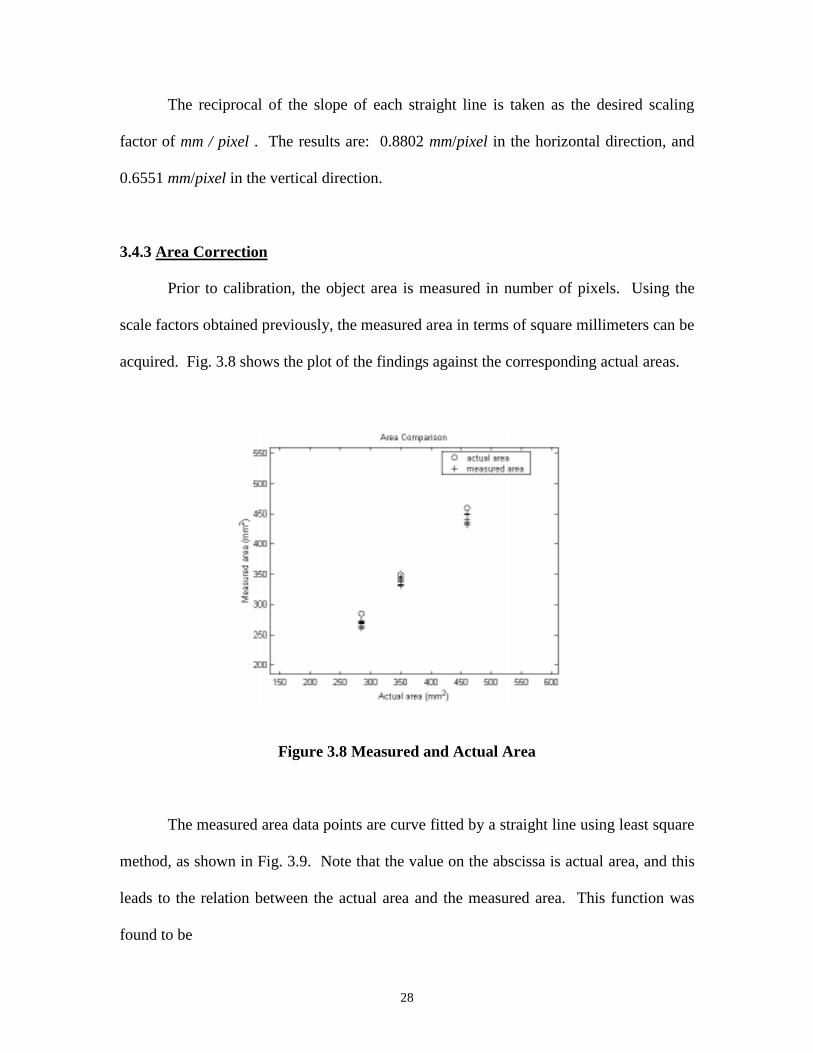
Prior to calibration, the object area is measured in number of pixels. Using the
scale factors obtained previously, the measured area in terms of square millimeters can be
acquired. Fig. 3.8 shows the plot of the findings against the corresponding actual areas.
Figure 3.8 Measured and Actual Area
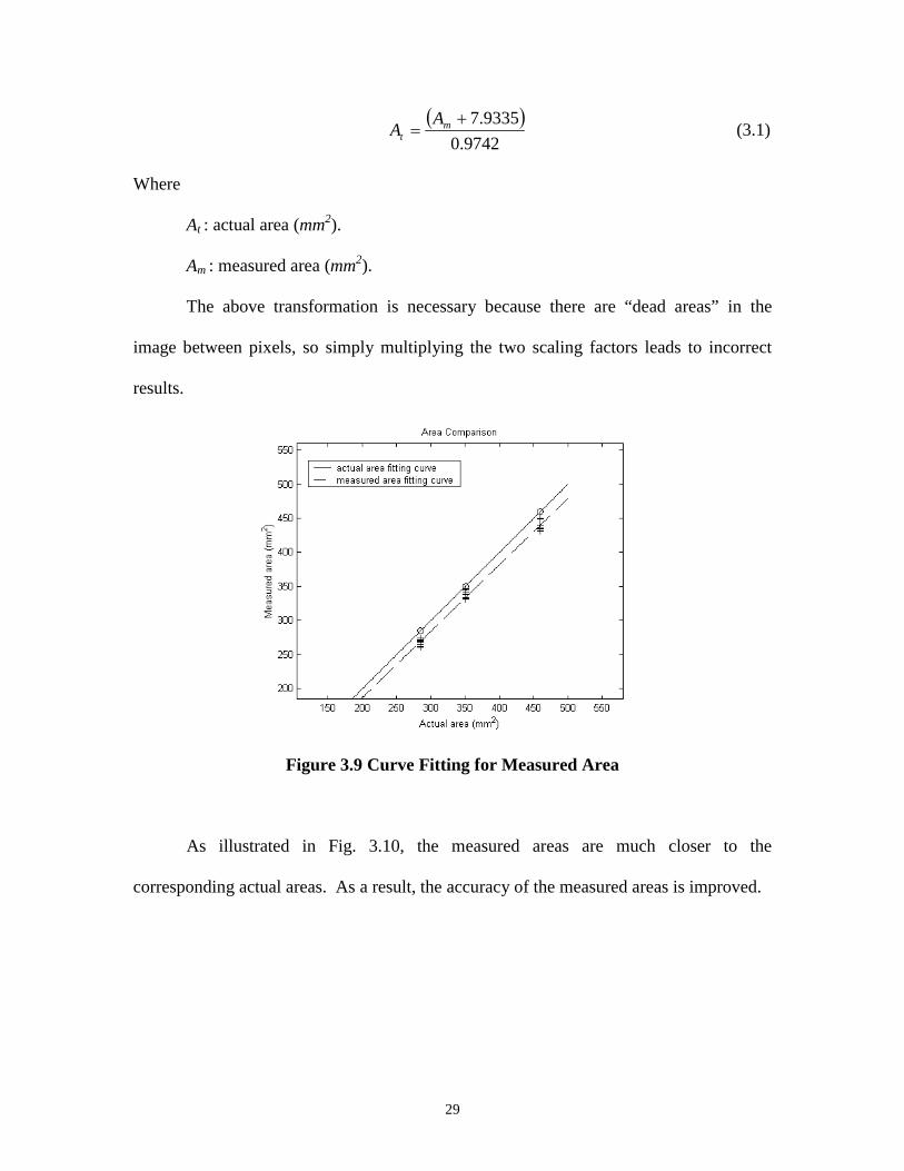
The measured area data points are curve fitted by a straight line using least square
method, as shown in Fig. 3.9. Note that the value on the abscissa is actual area, and this
leads to the relation between the actual area and the measured area. This function was
found to be
29
� �
9742.0
9335.7�
�m
t
AA (3.1)
Where
At : actual area (mm2).
Am : measured area (mm2).
The above transformation is necessary because there are “dead areas” in the
image between pixels, so simply multiplying the two scaling factors leads to incorrect
results.
Figure 3.9 Curve Fitting for Measured Area
As illustrated in Fig. 3.10, the measured areas are much closer to the
corresponding actual areas. As a result, the accuracy of the measured areas is improved.
30
Figure 3.10 Improvement of Measured Area
The improvement in the measured areas can be demonstrated by observing their
absolute percent error before and after using Eqn. (3.1). The absolute percent error for
three circle samples are shown in Fig. 3.11.
(a) absolute percent error for pennies
31
(b) absolute percent error for nickels
(c) absolute percent error for quarters
Figure 3.11 Absolute Percent Error Improvement
32
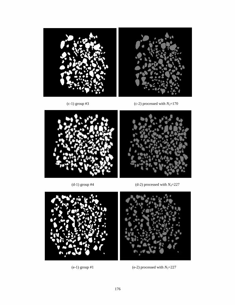
4. IMAGE PROCESSING AND ANALYSIS
4.1 Introduction
For each imaged object, that is, a non-touching-overlapping particle, the size and
shape as well as some other parameters must be computed for the particle volume
estimation and optical sieving purposes. Based upon the binary images – all particles are
white and background is black, the area, size, shape, and some other related statistics are
calculated. Image preprocessing includes binary conversion, edge detection, and
separation of the touching and overlapping particle shapes. By image analysis herein, it
means finding the particle shape centroid, area, major and minor diameters, identifying
shapes, and computing all the needed statistics of the particle in question.
Solution for finding above measurements is summarized in actual research
sequence as follows:
1) Binary image conversion.
2) Image capturing and seeding
3) Edge detection, region growing and particle projected area calculation.
4) Centroid location.
5) Major and minor diameter computation.
6) Particle profile shape characterization.
Successful completion of the image preprocessing and analysis paves the way to
establishing a mathematical model to estimate the volume of particle, and ultimately, to
obtain the particle size distribution through a sieving correlation process.
33
4.2 General Description
Fig. 4.1 shows images of four simulated particles. Sub-figure (a) simulates the
binary image that is the result of image processing, while (b) shows the completion of
the analysis to it. Once the particles have been converted to binary images and separated,
analysis starts with horizontal scanning and tracking the edge of each particle. During
the edge following, edge points (or pixels) are stored in an ordered list, and the interior
points are counted to compute the projected area of the particle. Calibrated scaling
factors are used to transform pixel numbers into dimensional measurements. The
centroid of the particle is calculated during the scanning process, and the pixels
belonging to the particle under consideration are labeled so they can be eliminated from
future scans.
(a) (b)
Figure 4.1 Simulated Particles with Centroid,Edges and Interior Points Labeled
Once this process is done, the list of edge points is sampled and the Euclidean
distance from the centroid to each of the edge points is computed. Because particle sizes
vary significantly, the sampling algorithm may be set up to choose an adequate number
of points from the edge to yield a good description of the particle silhouette in oder to
34
minimize the amount of computation required per particle. In this research, each edge
point is sampled. This sampling method results in samples at uneven intervals of the
polar angle � from the centroid, but avoids the time-consuming search for points
satisfying the angle interval criterion and the repeated calculation of the inverse tangent
function.
To characterize the particle’s profile shape, the “edge signature” is constructed. A
signature gives the distance between each edge point and the centroid, or, the radius at
each edge point, so the information about the particle’s shape can be stored in the
signature function. To eliminate the noise, the signature function is fitted by a
polynomial. Since the order of the polynomial is lower than the number of signature
points, significant smoothing of the curve occurs, yet the polynomial is complex enough
to track even relatively jagged particle boundaries accurately. The maxima and minima
of the polynomial can be computed, as can the sum of squared errors between the actual
signature points and the fitted curve. In general, maxima of the polynomial corespond to
the vertices of the particle, and the “significant” minima are often created by flat faces, as
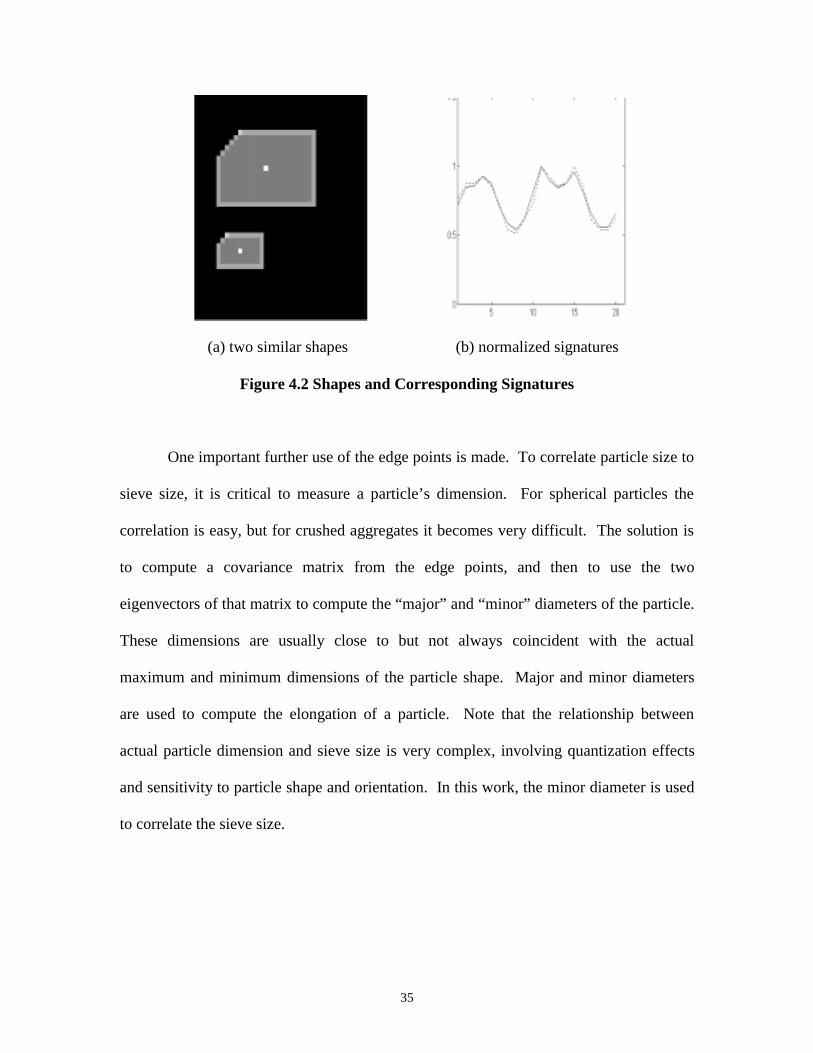
demonstrated in Fig. 4.2.
35
(a) two similar shapes (b) normalized signatures
Figure 4.2 Shapes and Corresponding Signatures
One important further use of the edge points is made. To correlate particle size to
sieve size, it is critical to measure a particle’s dimension. For spherical particles the
correlation is easy, but for crushed aggregates it becomes very difficult. The solution is
to compute a covariance matrix from the edge points, and then to use the two
eigenvectors of that matrix to compute the “major” and “minor” diameters of the particle.
These dimensions are usually close to but not always coincident with the actual
maximum and minimum dimensions of the particle shape. Major and minor diameters
are used to compute the elongation of a particle. Note that the relationship between
actual particle dimension and sieve size is very complex, involving quantization effects
and sensitivity to particle shape and orientation. In this work, the minor diameter is used
to correlate the sieve size.
36
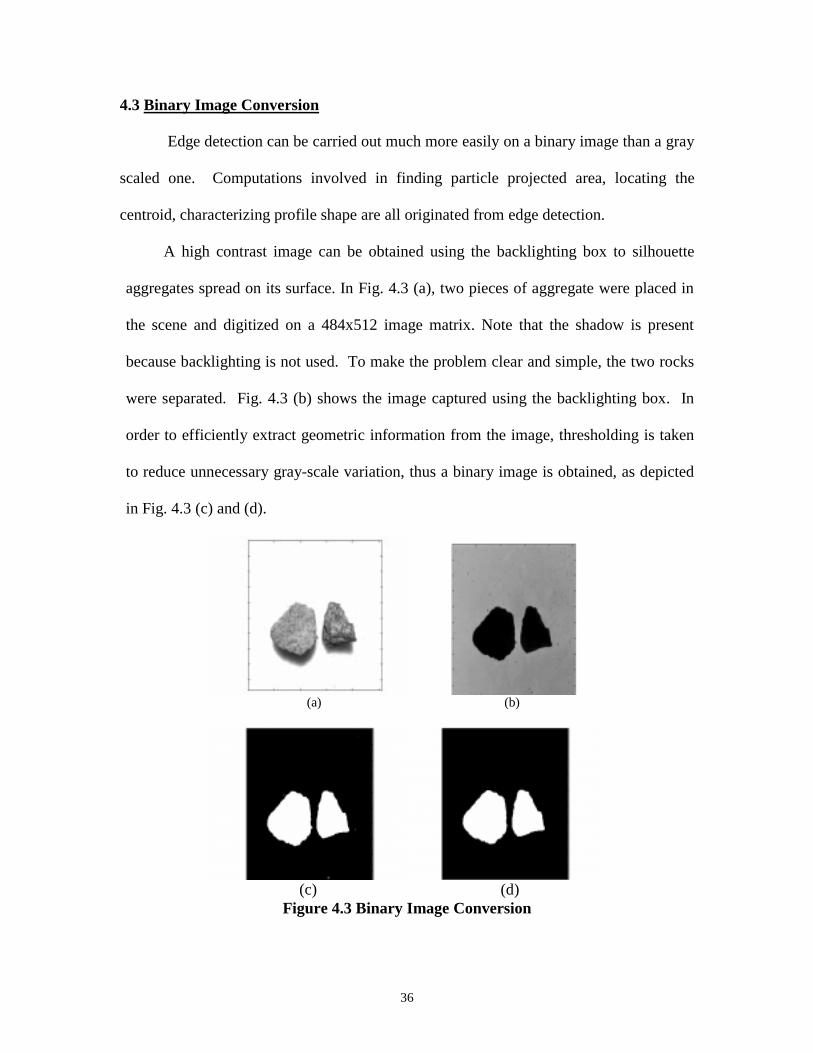
4.3 Binary Image Conversion
Edge detection can be carried out much more easily on a binary image than a gray
scaled one. Computations involved in finding particle projected area, locating the
centroid, characterizing profile shape are all originated from edge detection.
A high contrast image can be obtained using the backlighting box to silhouette
aggregates spread on its surface. In Fig. 4.3 (a), two pieces of aggregate were placed in
the scene and digitized on a 484x512 image matrix. Note that the shadow is present
because backlighting is not used. To make the problem clear and simple, the two rocks
were separated. Fig. 4.3 (b) shows the image captured using the backlighting box. In
order to efficiently extract geometric information from the image, thresholding is taken
to reduce unnecessary gray-scale variation, thus a binary image is obtained, as depicted
in Fig. 4.3 (c) and (d).
(a) (b)
(c) (d) Figure 4.3 Binary Image Conversion
37
Fig. (a): Image captured without using lighting box. Particle edges can be difficult to
distinguish from shadows.
Fig. (b): Image captured using lighting box. Conversion to binary image is carried out
on this image.
Fig. (c) (d): binary image obtained, before and after removal of small speckle noise. The
speckle noises can be caused by both insignificant tiny particles and unclean
camera lens. Checking the spot size experimentally can remove them.
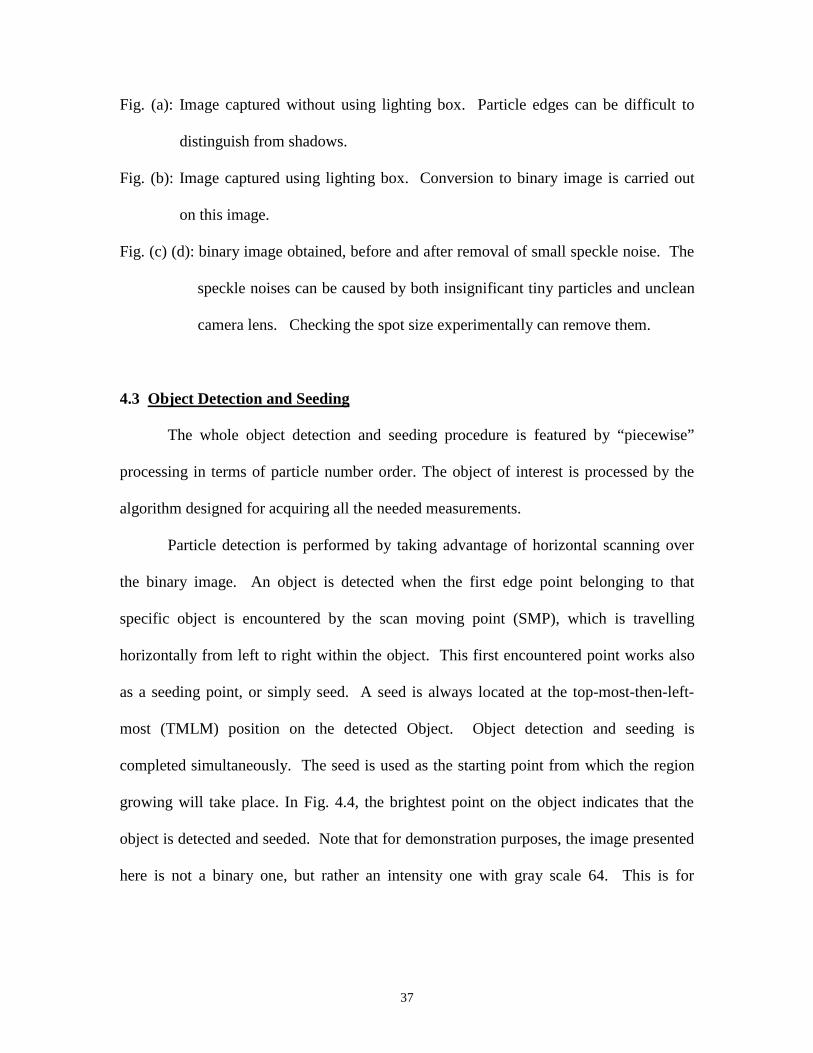
4.3 Object Detection and Seeding
The whole object detection and seeding procedure is featured by “piecewise”
processing in terms of particle number order. The object of interest is processed by the
algorithm designed for acquiring all the needed measurements.
Particle detection is performed by taking advantage of horizontal scanning over
the binary image. An object is detected when the first edge point belonging to that
specific object is encountered by the scan moving point (SMP), which is travelling
horizontally from left to right within the object. This first encountered point works also
as a seeding point, or simply seed. A seed is always located at the top-most-then-left-
most (TMLM) position on the detected Object. Object detection and seeding is
completed simultaneously. The seed is used as the starting point from which the region
growing will take place. In Fig. 4.4, the brightest point on the object indicates that the
object is detected and seeded. Note that for demonstration purposes, the image presented
here is not a binary one, but rather an intensity one with gray scale 64. This is for
38
showing up the seed location. In fact, pixel labeling is imbedded throughout the
algorithm for various processing purposes.
Figure 4.4 Object Detected and Seeded
In the multi-object case, an object whose TMLM edge point is also in the top-
most and left-most position in the image matrix, will be detected and seeded first, since
the SMP is traveling rightward, and the scan line is moving downward. Once the object’s
last pixel has been encountered by SMP, this object is isolated from all other objects,
processed and would-be-processed alike, in order to avoid being re-encountered by the
SMP. The detail about isolation is given in the later section. The processed object can
also be considered as having been converted to the background, and it will be ignored by
the SMP. The next candidate object to be detected and seeded is the one whose TMLM
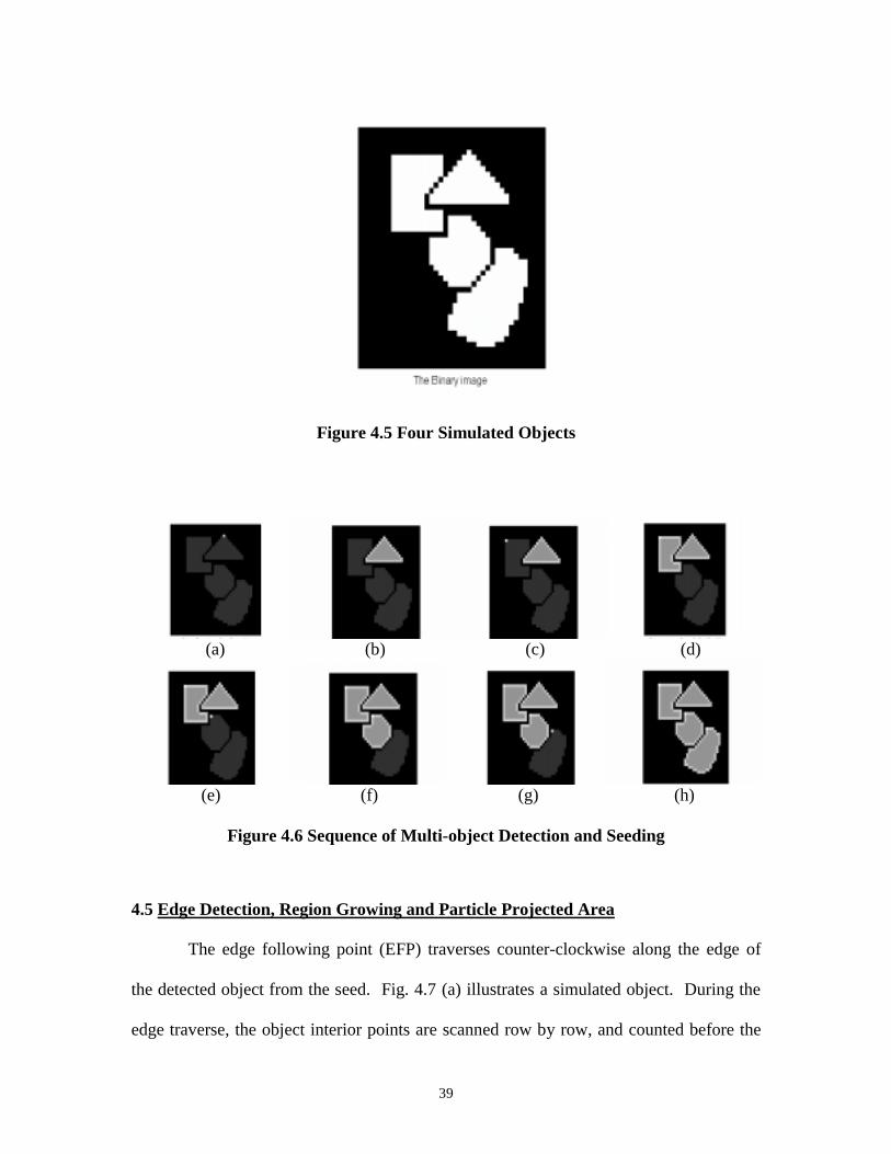
edge point satisfies the position conditions for detection priority. Fig. 4.5 shows four
simulated overlapped but separated objects. Fig. 4.6 illustrates the sequence of detection
and seeding for these four objects.
39
Figure 4.5 Four Simulated Objects
(a) (b) (c) (d)
(e) (f) (g) (h)
Figure 4.6 Sequence of Multi-object Detection and Seeding
4.5 Edge Detection, Region Growing and Particle Projected Area
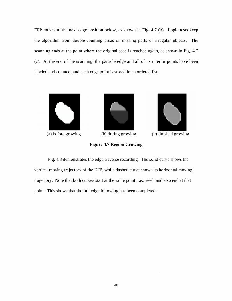
The edge following point (EFP) traverses counter-clockwise along the edge of
the detected object from the seed. Fig. 4.7 (a) illustrates a simulated object. During the
edge traverse, the object interior points are scanned row by row, and counted before the
40
EFP moves to the next edge position below, as shown in Fig. 4.7 (b). Logic tests keep
the algorithm from double-counting areas or missing parts of irregular objects. The
scanning ends at the point where the original seed is reached again, as shown in Fig. 4.7
(c). At the end of the scanning, the particle edge and all of its interior points have been
labeled and counted, and each edge point is stored in an ordered list.
(a) before growing (b) during growing (c) finished growing
Figure 4.7 Region Growing
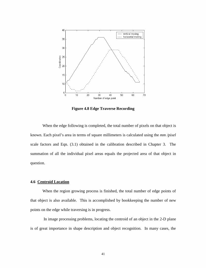
Fig. 4.8 demonstrates the edge traverse recording. The solid curve shows the
vertical moving trajectory of the EFP, while dashed curve shows its horizontal moving
trajectory. Note that both curves start at the same point, i.e., seed, and also end at that
point. This shows that the full edge following has been completed.
41
Figure 4.8 Edge Traverse Recording
When the edge following is completed, the total number of pixels on that object is
known. Each pixel’s area in terms of square millimeters is calculated using the mm /pixel
scale factors and Eqn. (3.1) obtained in the calibration described in Chapter 3. The
summation of all the individual pixel areas equals the projected area of that object in
question.
4.6 Centroid Location
When the region growing process is finished, the total number of edge points of
that object is also available. This is accomplished by bookkeeping the number of new
points on the edge while traversing is in progress.
In image processing problems, locating the centroid of an object in the 2-D plane
is of great importance in shape description and object recognition. In many cases, the
42
centroid is used as a reference point to which the position of other points in question can
be determined.
For a function f(x,y), the moment of order (p+q) is defined as mpq, and the
centroid coordinates can be found at
mmx
00
10� (4.1)
mmy
00
01� (4.2)
where, for a digital image,
���
�
�
�
�1
0
1
000
),(n
y
m
x
yxfm (4.3)
���
�
�
�
�1
0
1
010
),(n
x
m
y
yxxfm (4.4)
���
�
�
�
�1
0
1
001
),(n
y
m
x
yxyfm (4.5)
where x and y indicate the coordinates of the image matrix.
Emdedding Eqn. (4.1) ~ (4.5) in the algrithm, the position of the centroid for each
individual shape in the image is located. The centroid finding procedure now is applied
to the real image as shown in Fig. 4.9.
43
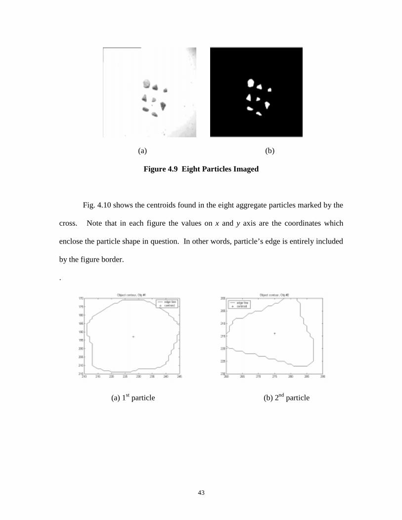
(a) (b)
Figure 4.9 Eight Particles Imaged
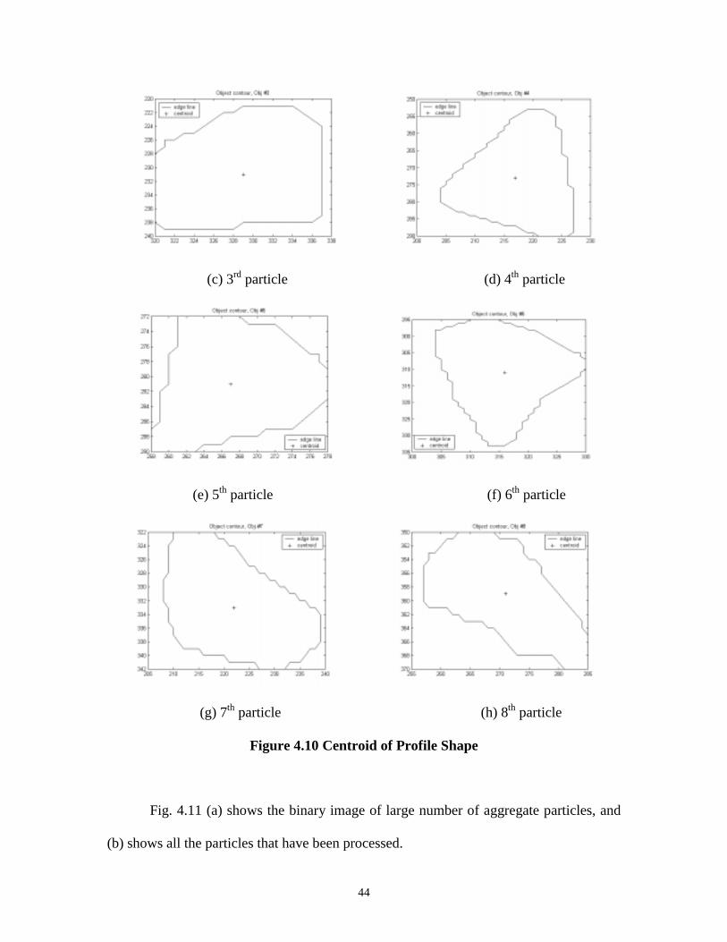
Fig. 4.10 shows the centroids found in the eight aggregate particles marked by the
cross. Note that in each figure the values on x and y axis are the coordinates which
enclose the particle shape in question. In other words, particle’s edge is entirely included
by the figure border.
.
(a) 1st particle (b) 2nd particle
44
(c) 3rd particle (d) 4th particle
(e) 5th particle (f) 6th particle
(g) 7th particle (h) 8th particle
Figure 4.10 Centroid of Profile Shape
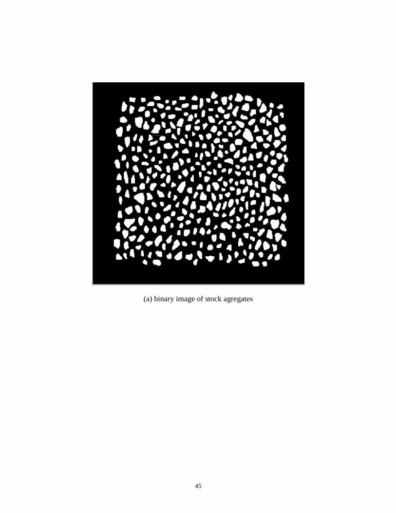
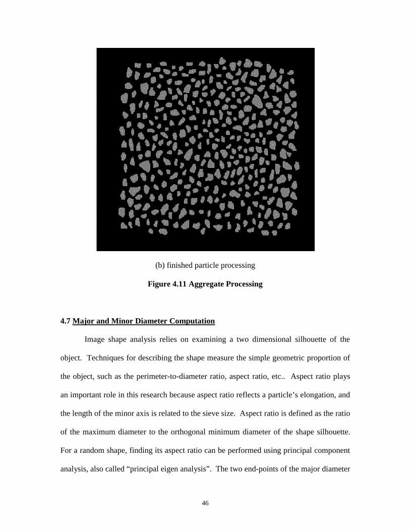
Fig. 4.11 (a) shows the binary image of large number of aggregate particles, and
(b) shows all the particles that have been processed.
45
(a) binary image of stock agregates
46
(b) finished particle processing
Figure 4.11 Aggregate Processing
4.7 Major and Minor Diameter Computation
Image shape analysis relies on examining a two dimensional silhouette of the
object. Techniques for describing the shape measure the simple geometric proportion of
the object, such as the perimeter-to-diameter ratio, aspect ratio, etc.. Aspect ratio plays
an important role in this research because aspect ratio reflects a particle’s elongation, and
the length of the minor axis is related to the sieve size. Aspect ratio is defined as the ratio
of the maximum diameter to the orthogonal minimum diameter of the shape silhouette.
For a random shape, finding its aspect ratio can be performed using principal component
analysis, also called “principal eigen analysis”. The two end-points of the major diameter
47
must be on the major eigen axis, and the two end-points of the orthogonal minor diameter
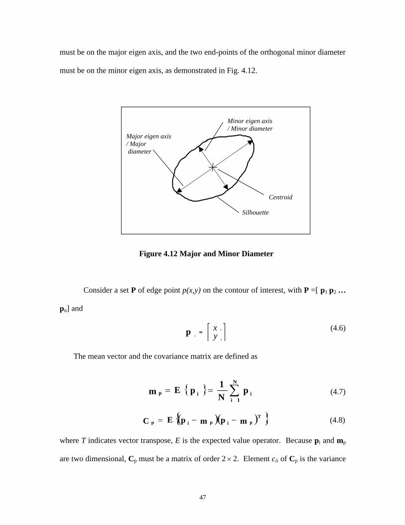
must be on the minor eigen axis, as demonstrated in Fig. 4.12.
Figure 4.12 Major and Minor Diameter
Consider a set P of edge point p(x,y) on the contour of interest, with P =[ p1 p2 …
pn] and
���
�
���
�� y
xi
i
ip (4.6)
The mean vector and the covariance matrix are defined as
� � ��
��N
1iiip p
N1
p Em (4.7)
� �� �� �Tpipip mpmpEC ��� (4.8)
where T indicates vector transpose, E is the expected value operator. Because pi and mp
are two dimensional, Cp must be a matrix of order 2� 2. Element cii of Cp is the variance
Minor eigen axis / Minor diameterMajor eigen axis/ Major diameter
Centroid
Silhouette
48
of x and y in pi, and element cij of Cp is the covariance between x and y. The matrix Cp
is real and symmetric.
For M vector samples, namely, M edge points, the mean vector and covariance
matrix are computed as
��
�
M
iiM 1
p1m p
(4.9)
)1
1( mmppC ppp
TT
i
M
iiM
�� ��
(4.10)
Because the matrix Cp is real and symmetric, finding a set of orthogonal eigenvectors of
dimension 2 is always possible [2]. Let �1 and �2 be the eigenvalues of Cp, with �1>�2,
and correspondingly, let e1 and e2 be the resultant eigenvectors. The direction of vector e1
indicates the orientation of the particle’s major eigen axis, and likewise, the direction of
e2 coincides with the direction of its minor eigen axis. The end-points of the major and
minor axes within the contour can be found, so that the major diameter and its orthogonal
minor diameter can thus be obtained.
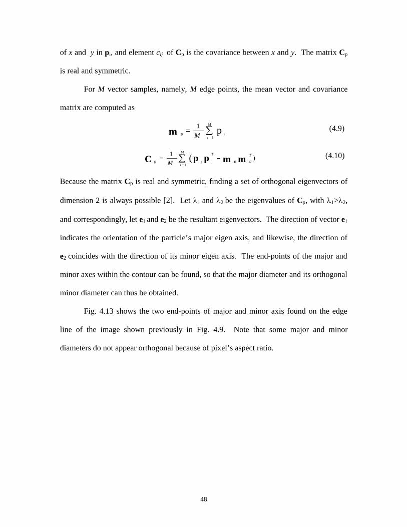
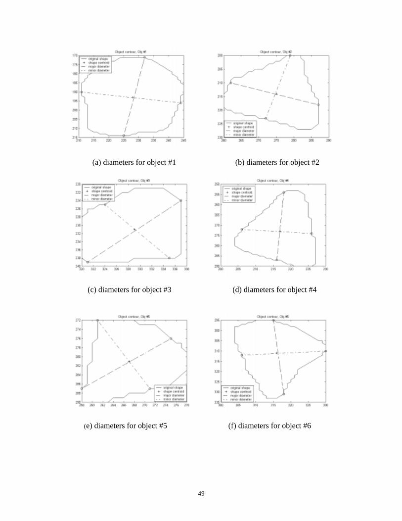
Fig. 4.13 shows the two end-points of major and minor axis found on the edge
line of the image shown previously in Fig. 4.9. Note that some major and minor
diameters do not appear orthogonal because of pixel’s aspect ratio.
49
(a) diameters for object #1 (b) diameters for object #2
(c) diameters for object #3 (d) diameters for object #4
(e) diameters for object #5 (f) diameters for object #6
50
( g) diameters for object #7 (h) diameters for object #8
Figure 4.13 Major and Minor Diameter
After obtaining the major and minor diameter, the aspect ratio of the profile shape
of the particle is computed.
4.8 Profile Shape Characterization
The major reason for needing to know the approximate shape of the particles lies
in the fact that shape affects the strategy for converting the particle profile into an
equivalent sieve size. For example, rectangular particles will sieve to the smaller of the
two dimensions, which can be found approximately using the minor diameter. On the
other hand, a triangular shaped particle will sieve to one vertex and the opposite side, the
length that is sieved to is greater than the minor diameter of the profile shape. This
requires modification of the minor diameter.
Using the list of edge points to plot the radius from the centroid to each edge
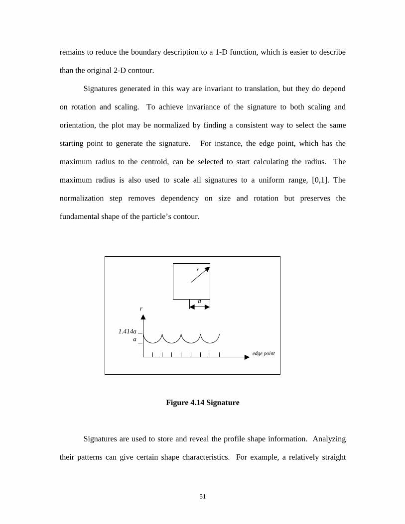
point, a relation called “signature” is constructed. Fig. 4.14 illustrates such a functional
relation for a square. Irrespective of how such a signature is created, the basic idea
51
remains to reduce the boundary description to a 1-D function, which is easier to describe
than the original 2-D contour.
Signatures generated in this way are invariant to translation, but they do depend
on rotation and scaling. To achieve invariance of the signature to both scaling and
orientation, the plot may be normalized by finding a consistent way to select the same
starting point to generate the signature. For instance, the edge point, which has the
maximum radius to the centroid, can be selected to start calculating the radius. The
maximum radius is also used to scale all signatures to a uniform range, [0,1]. The
normalization step removes dependency on size and rotation but preserves the
fundamental shape of the particle’s contour.
Figure 4.14 Signature
Signatures are used to store and reveal the profile shape information. Analyzing
their patterns can give certain shape characteristics. For example, a relatively straight
a r
1.414a a
edge point
r
52
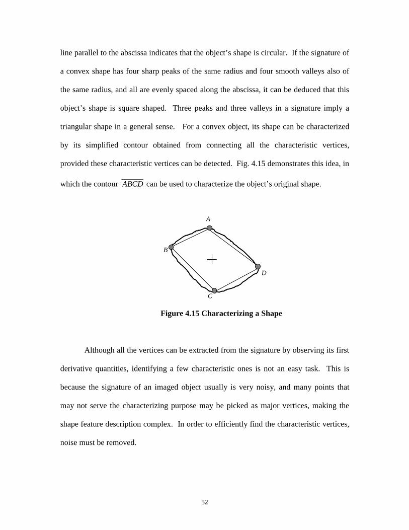
line parallel to the abscissa indicates that the object’s shape is circular. If the signature of
a convex shape has four sharp peaks of the same radius and four smooth valleys also of
the same radius, and all are evenly spaced along the abscissa, it can be deduced that this
object’s shape is square shaped. Three peaks and three valleys in a signature imply a
triangular shape in a general sense. For a convex object, its shape can be characterized
by its simplified contour obtained from connecting all the characteristic vertices,
provided these characteristic vertices can be detected. Fig. 4.15 demonstrates this idea, in
which the contour ABCD can be used to characterize the object’s original shape.
Figure 4.15 Characterizing a Shape
Although all the vertices can be extracted from the signature by observing its first
derivative quantities, identifying a few characteristic ones is not an easy task. This is
because the signature of an imaged object usually is very noisy, and many points that
may not serve the characterizing purpose may be picked as major vertices, making the
shape feature description complex. In order to efficiently find the characteristic vertices,
noise must be removed.
A
B
D
C
53
Polynomial curve-fitting can effectively approximate functions (interpolating
polynomials) to smooth out noisy experimental and numerical data, and provide a simple
analytical expression. The most commonly chosen form is the polynomial:
g(x)=a0 xp+ a1 x
p-1+ a2 xp-2+ a3 x
p-3+ … + ap-2 x2+ ap-1 x+ap (4.11)
where x is the variable of edge points.
Determination of the order of the polynomial p is problem dependent. For a given
set of data points, an order too high causes detection of unwanted and insignificant
vertices, an order too low lacks sensitivity of detection. After trial-and-error, p=18 was
selected in this research. After the order was chosen, the first derivative of the
polynomial was taken to identify characteristic vertices, using:
0)(�
dx
xdg (4.12)
to locate the positions of the desired vertices on the original signature. The number of
maxima and minima is an indicator to the number of “corners” and “sides” that the
particle has.
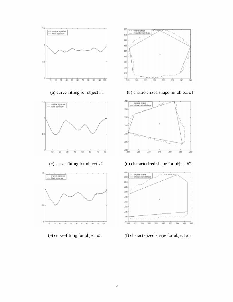
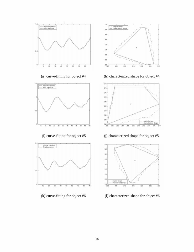
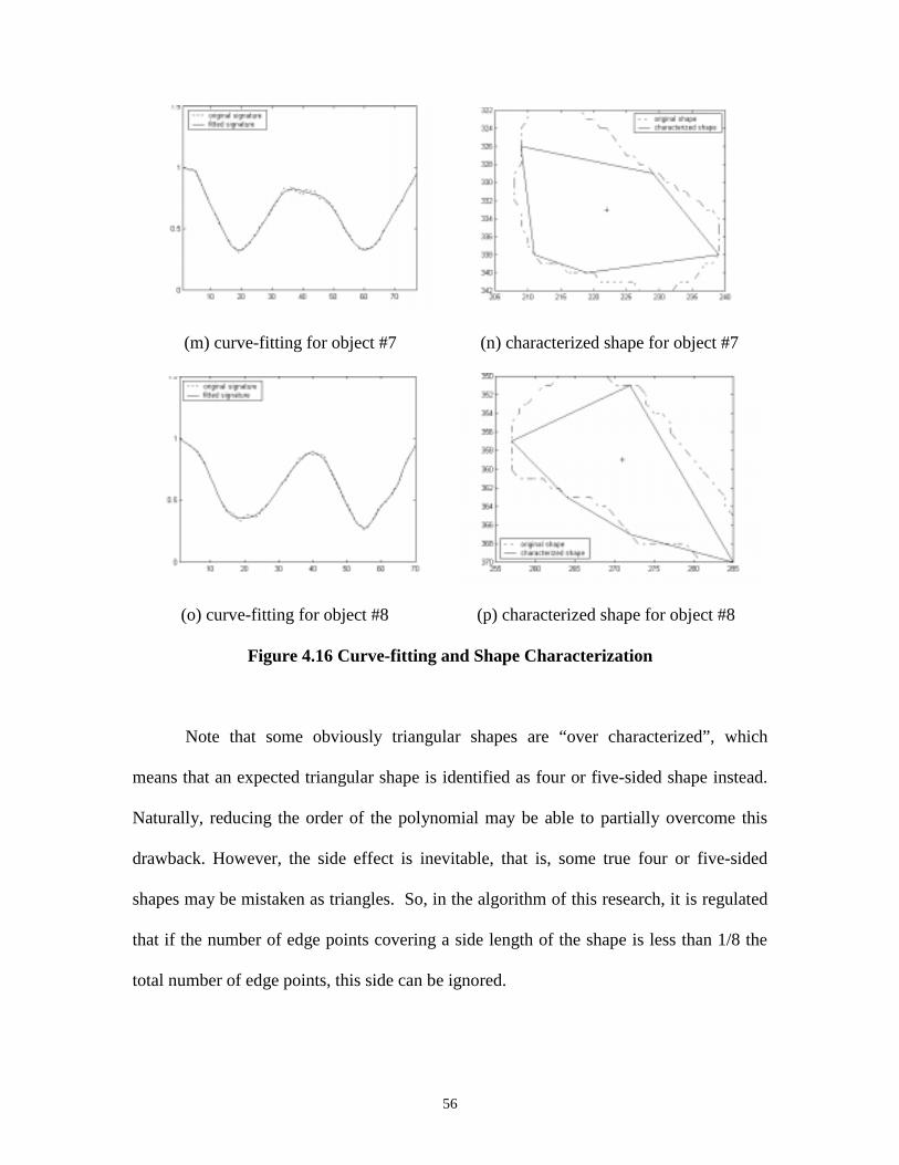
Now, taking the same images as shown in Fig. 4.9, the selected polynomial is
applied to identify these eight particles’ profile shape. Fig. 4.16 demonstrates the results.
All plots in the left column show the polynomial curve-fitting effect, and shapes
identified on the other.
54
(a) curve-fitting for object #1 (b) characterized shape for object #1
(c) curve-fitting for object #2 (d) characterized shape for object #2
(e) curve-fitting for object #3 (f) characterized shape for object #3
55
(g) curve-fitting for object #4 (h) characterized shape for object #4
(i) curve-fitting for object #5 (j) characterized shape for object #5
(k) curve-fitting for object #6 (l) characterized shape for object #6
56
(m) curve-fitting for object #7 (n) characterized shape for object #7
(o) curve-fitting for object #8 (p) characterized shape for object #8
Figure 4.16 Curve-fitting and Shape Characterization
Note that some obviously triangular shapes are “over characterized”, which
means that an expected triangular shape is identified as four or five-sided shape instead.
Naturally, reducing the order of the polynomial may be able to partially overcome this
drawback. However, the side effect is inevitable, that is, some true four or five-sided
shapes may be mistaken as triangles. So, in the algorithm of this research, it is regulated
that if the number of edge points covering a side length of the shape is less than 1/8 the
total number of edge points, this side can be ignored.
57
5. SEPARATION OF TOUCHING AND
OVERLAPPING PARTICLES
5.1 Introduction
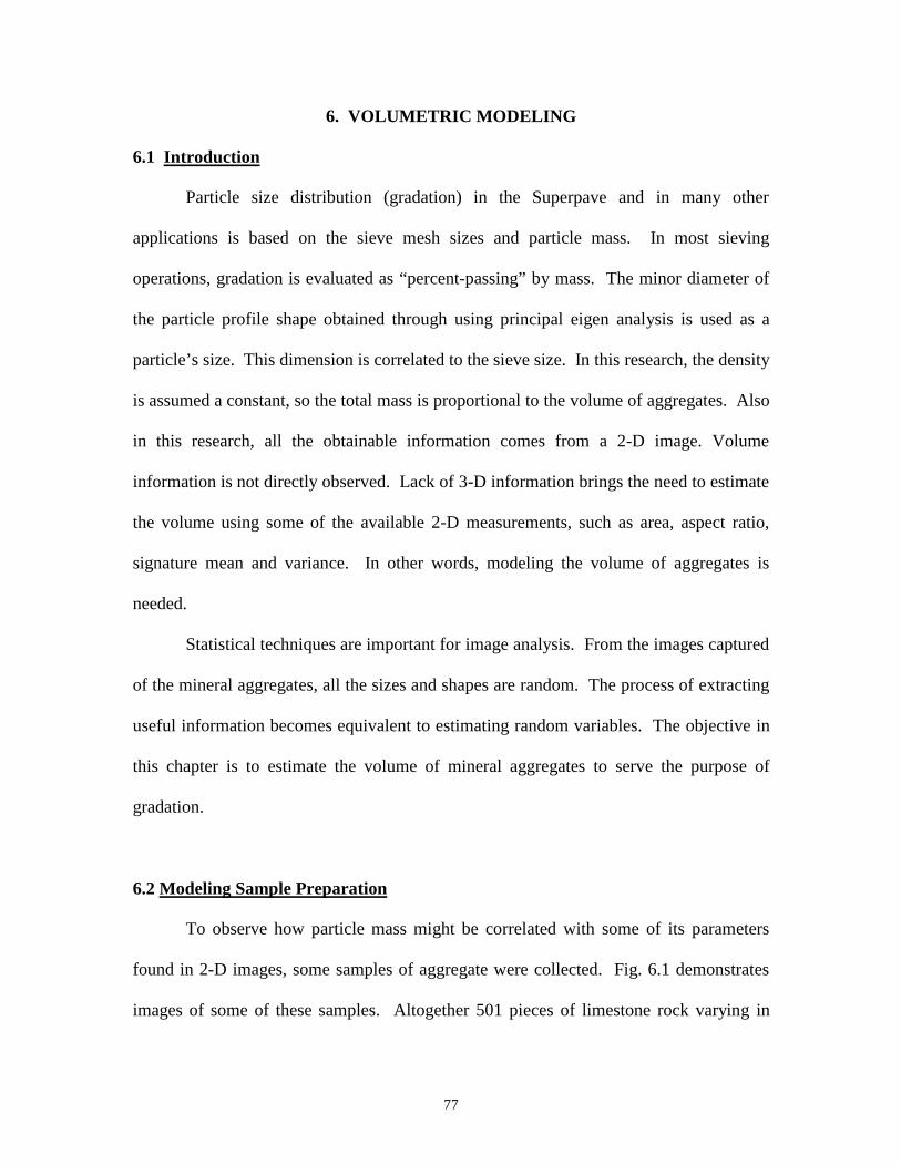
In the processing of aggregate particle images, two problems must be solved
before size and shape analysis begin. First, if the particles are touching or overlapping,
two or more particles will appear as one large, irregularly shaped particle. Second, each
image consists of many individual particles, all of which must be processed individually
to determine particle size, shape and mass. These two problems demand separation of all
touching or overlapping particles before further analysis can be conducted on the image.
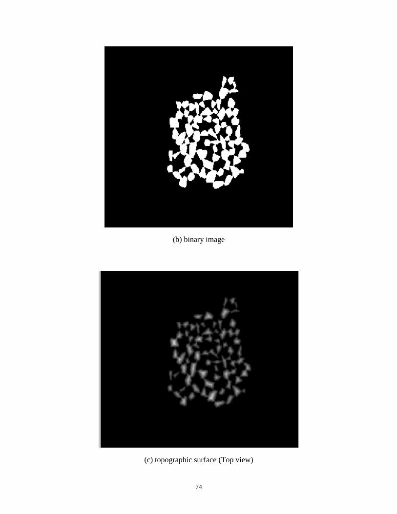
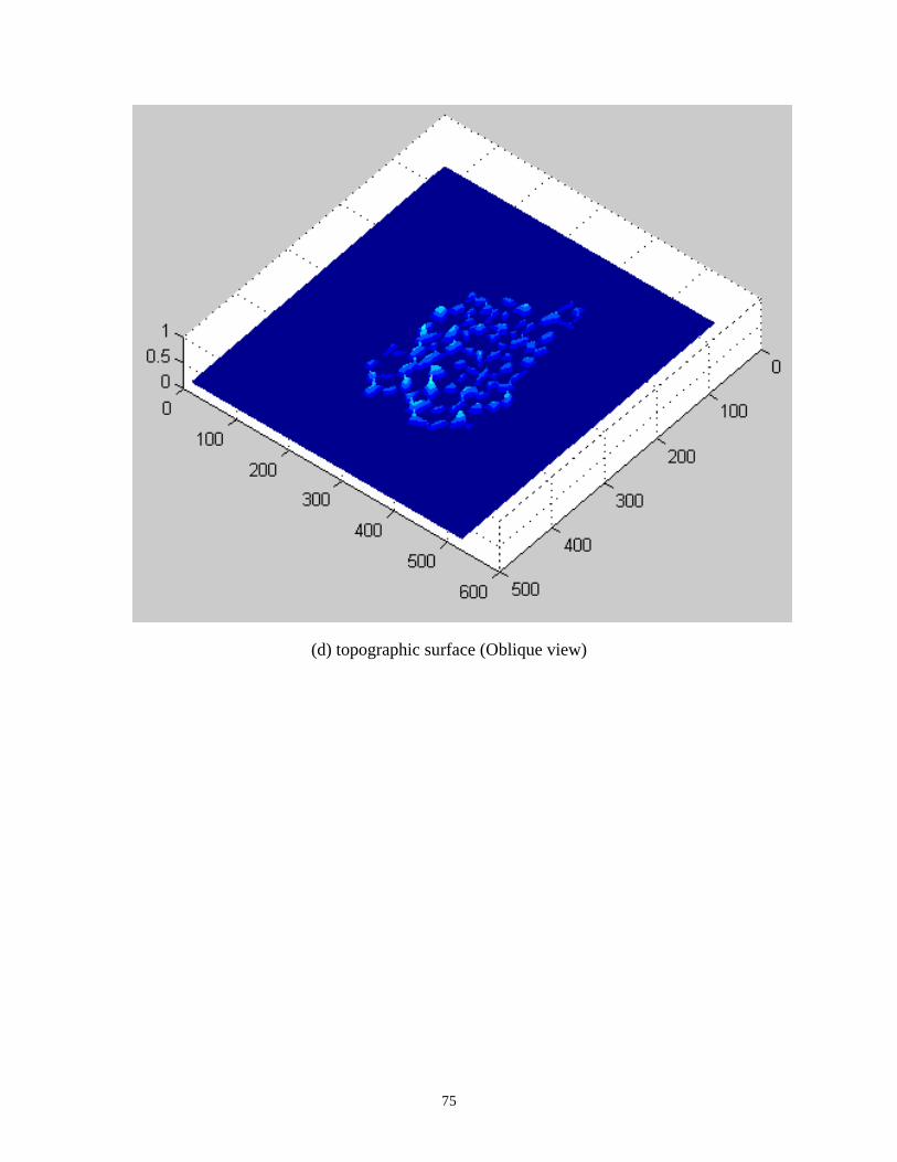
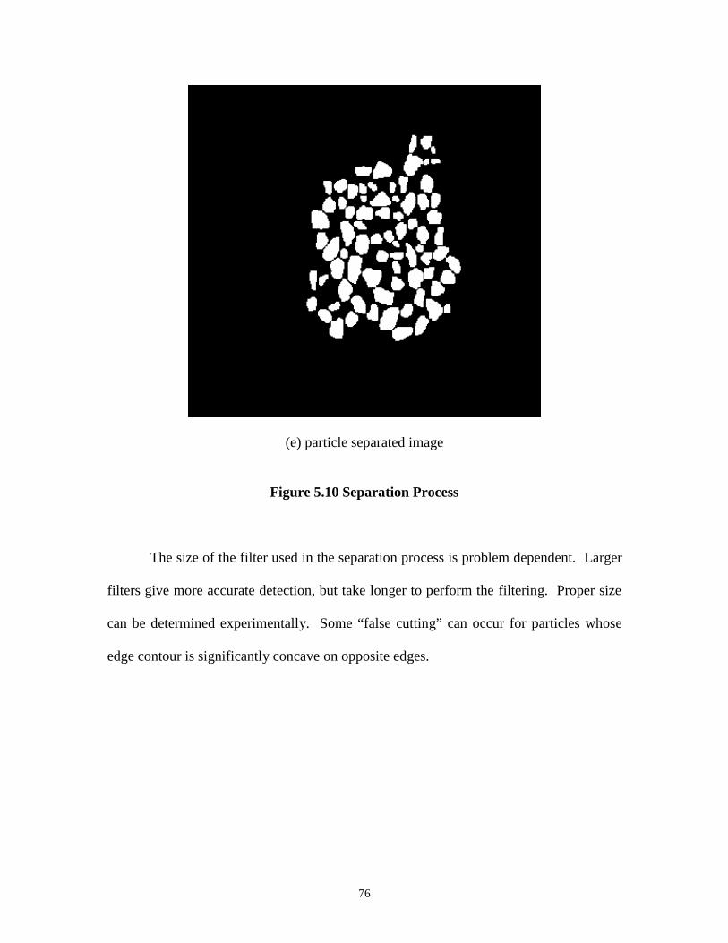
Morphological processing techniques can be used to convert the binary image to a
gray scale topographic surface [21]. In this chapter, some basic morphological concepts
are reviewed. The 3-D geometric characteristics existing between two touching or
overlapping objects are analyzed. A morphological erosion process is demonstrated,
which leads to finding a saddle point in a concave particle outline. A cut line is made
through the saddle point and eventually the two objects are separated.
5.2 Binary Erosion
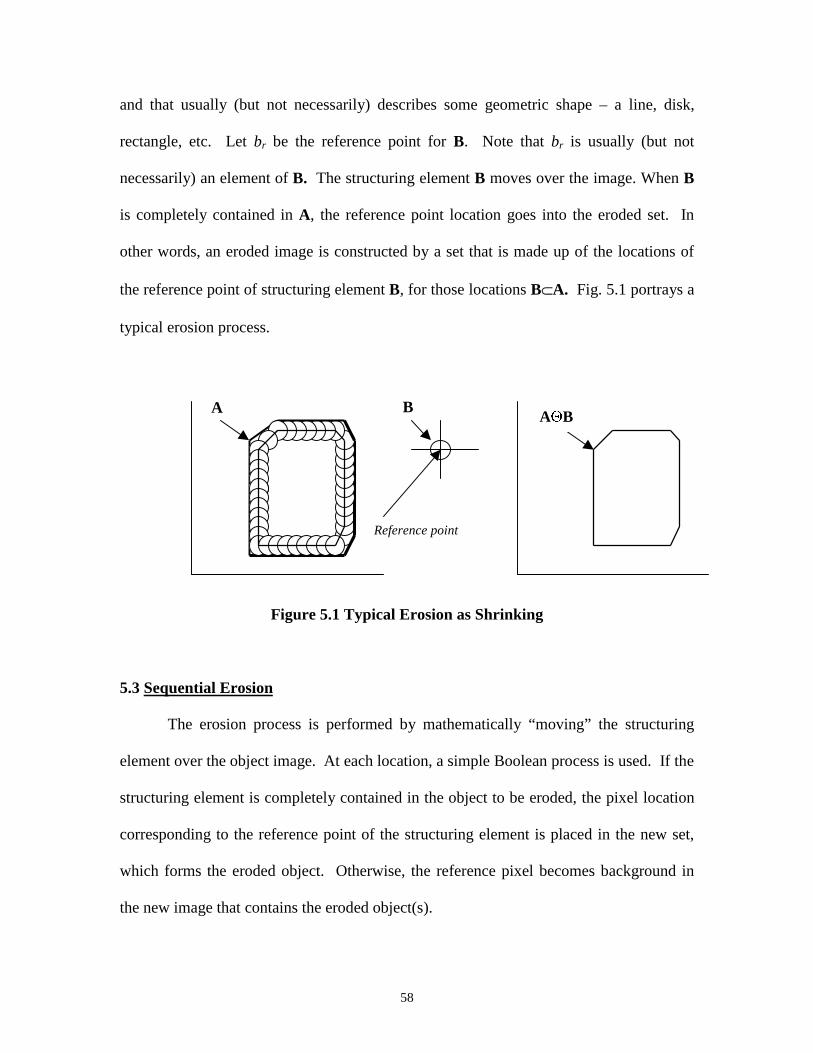
The fundamental operations of mathematical morphology are erosion and dilation.
In this work, erosion is the more important process, and can be described as follows:
suppose a binary image Im�n contains background pixels with value 0 and object pixels
with value 1. Assume that the object pixels are grouped into a single, contiguous object
A comprised of q pixels a1, a2, … aq, q�m�n. Let B={b1 b2 … bk } be a structuring
element, which is a set of binary points that are usually (but not necessarily) contiguous
58
and that usually (but not necessarily) describes some geometric shape – a line, disk,
rectangle, etc. Let br be the reference point for B. Note that br is usually (but not
necessarily) an element of B. The structuring element B moves over the image. When B
is completely contained in A, the reference point location goes into the eroded set. In
other words, an eroded image is constructed by a set that is made up of the locations of
the reference point of structuring element B, for those locations B�A. Fig. 5.1 portrays a
typical erosion process.
Figure 5.1 Typical Erosion as Shrinking
5.3 Sequential Erosion
The erosion process is performed by mathematically “moving” the structuring
element over the object image. At each location, a simple Boolean process is used. If the
structuring element is completely contained in the object to be eroded, the pixel location
corresponding to the reference point of the structuring element is placed in the new set,
which forms the eroded object. Otherwise, the reference pixel becomes background in
the new image that contains the eroded object(s).
A BBA�
Reference point
59
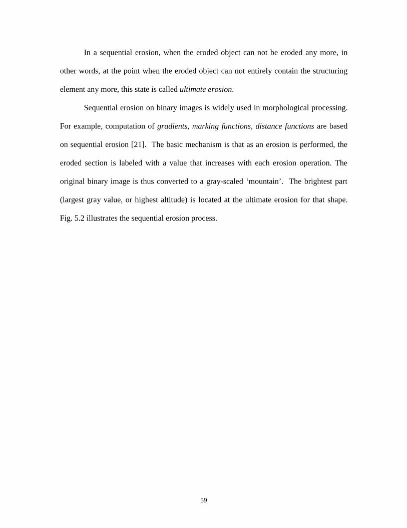
In a sequential erosion, when the eroded object can not be eroded any more, in
other words, at the point when the eroded object can not entirely contain the structuring
element any more, this state is called ultimate erosion.
Sequential erosion on binary images is widely used in morphological processing.
For example, computation of gradients, marking functions, distance functions are based
on sequential erosion [21]. The basic mechanism is that as an erosion is performed, the
eroded section is labeled with a value that increases with each erosion operation. The
original binary image is thus converted to a gray-scaled ‘mountain’. The brightest part
(largest gray value, or highest altitude) is located at the ultimate erosion for that shape.
Fig. 5.2 illustrates the sequential erosion process.
60
(a) original binary image
Gray value (label)
Altitude Altitude
(b) after ultimate erosion (oblique view)
(c) after ultimate erosion (top view: topographic surface)
Figure 5.2 Sequential Erosion
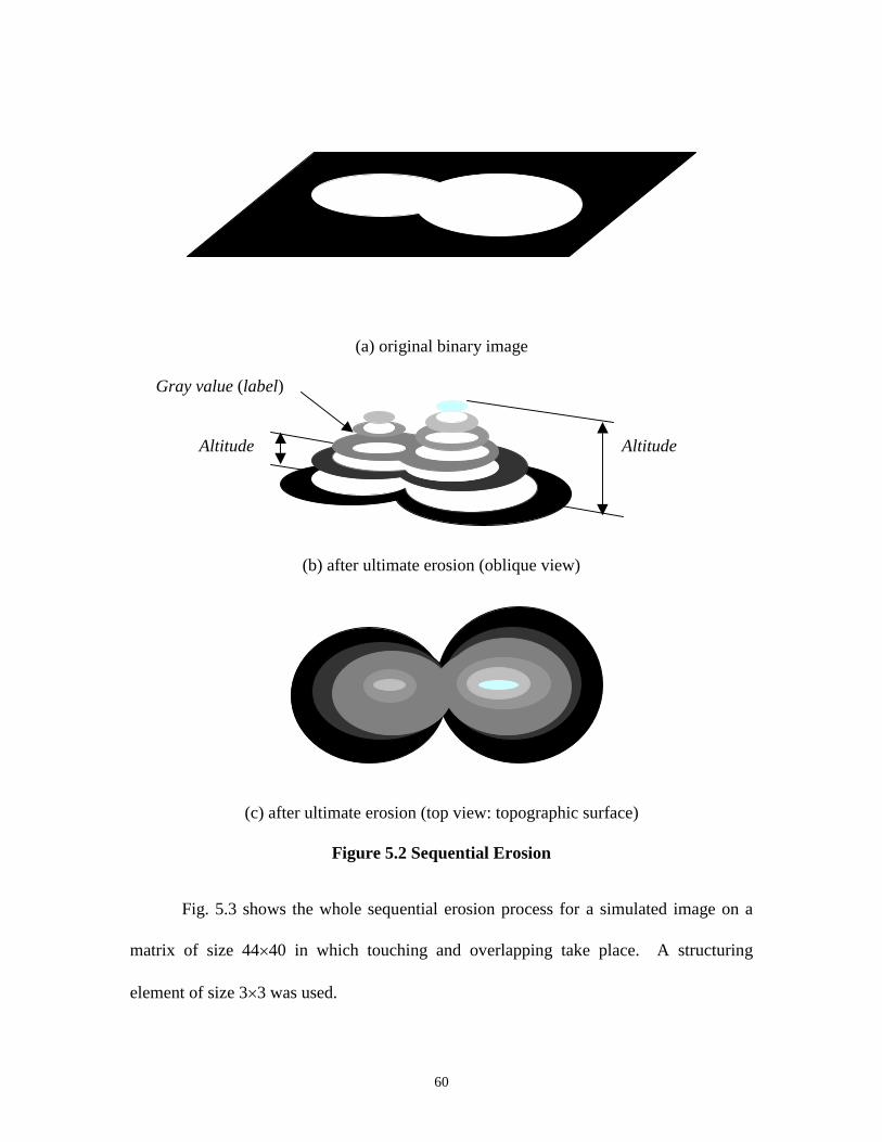
Fig. 5.3 shows the whole sequential erosion process for a simulated image on a
matrix of size 44�40 in which touching and overlapping take place. A structuring
element of size 3�3 was used.
61
(a) before erosion (b) 1st erosion
(c) 2nd erosion (d) 3rd erosion
(e) 4therosion (f) ultimate erosion
Figure 5.3 Sequential Erosion on Simulated Image
62
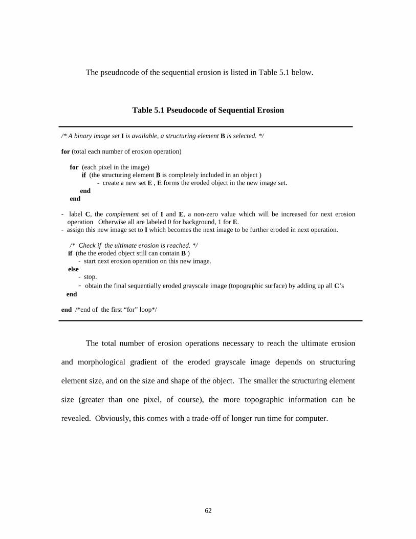
The pseudocode of the sequential erosion is listed in Table 5.1 below.
Table 5.1 Pseudocode of Sequential Erosion
/* A binary image set I is available, a structuring element B is selected. */
for (total each number of erosion operation)
for (each pixel in the image) if (the structuring element B is completely included in an object ) - create a new set E , E forms the eroded object in the new image set. end end
- label C, the complement set of I and E, a non-zero value which will be increased for next erosionoperation Otherwise all are labeled 0 for background, 1 for E.
- assign this new image set to I which becomes the next image to be further eroded in next operation.
/* Check if the ultimate erosion is reached. */ if (the the eroded object still can contain B ) - start next erosion operation on this new image. else - stop. - obtain the final sequentially eroded grayscale image (topographic surface) by adding up all C’s end
end /*end of the first “for” loop*/
The total number of erosion operations necessary to reach the ultimate erosion
and morphological gradient of the eroded grayscale image depends on structuring
element size, and on the size and shape of the object. The smaller the structuring element
size (greater than one pixel, of course), the more topographic information can be
revealed. Obviously, this comes with a trade-off of longer run time for computer.
63
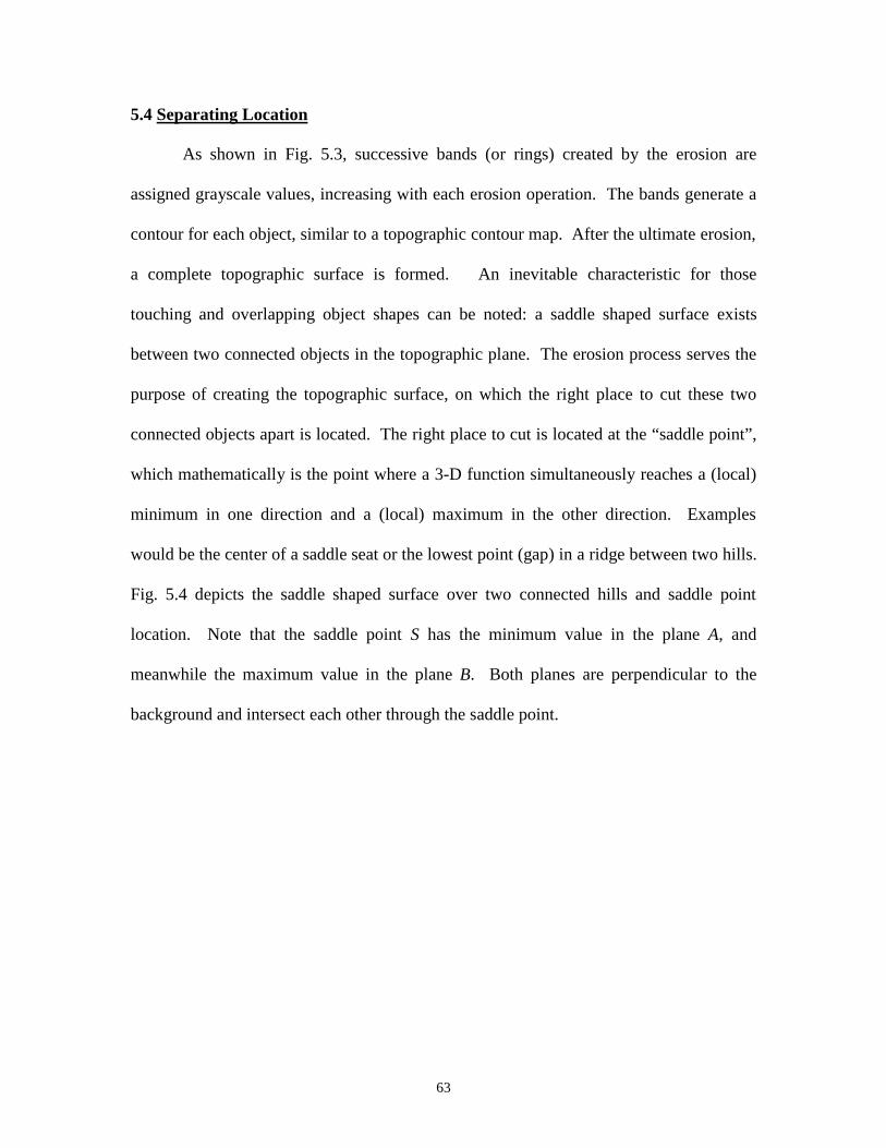
5.4 Separating Location
As shown in Fig. 5.3, successive bands (or rings) created by the erosion are
assigned grayscale values, increasing with each erosion operation. The bands generate a
contour for each object, similar to a topographic contour map. After the ultimate erosion,
a complete topographic surface is formed. An inevitable characteristic for those
touching and overlapping object shapes can be noted: a saddle shaped surface exists
between two connected objects in the topographic plane. The erosion process serves the
purpose of creating the topographic surface, on which the right place to cut these two
connected objects apart is located. The right place to cut is located at the “saddle point”,
which mathematically is the point where a 3-D function simultaneously reaches a (local)
minimum in one direction and a (local) maximum in the other direction. Examples
would be the center of a saddle seat or the lowest point (gap) in a ridge between two hills.
Fig. 5.4 depicts the saddle shaped surface over two connected hills and saddle point
location. Note that the saddle point S has the minimum value in the plane A, and
meanwhile the maximum value in the plane B. Both planes are perpendicular to the
background and intersect each other through the saddle point.
64
Plane B
Plane A Saddle Point S
Figure 5.4 Saddle and Saddle Point
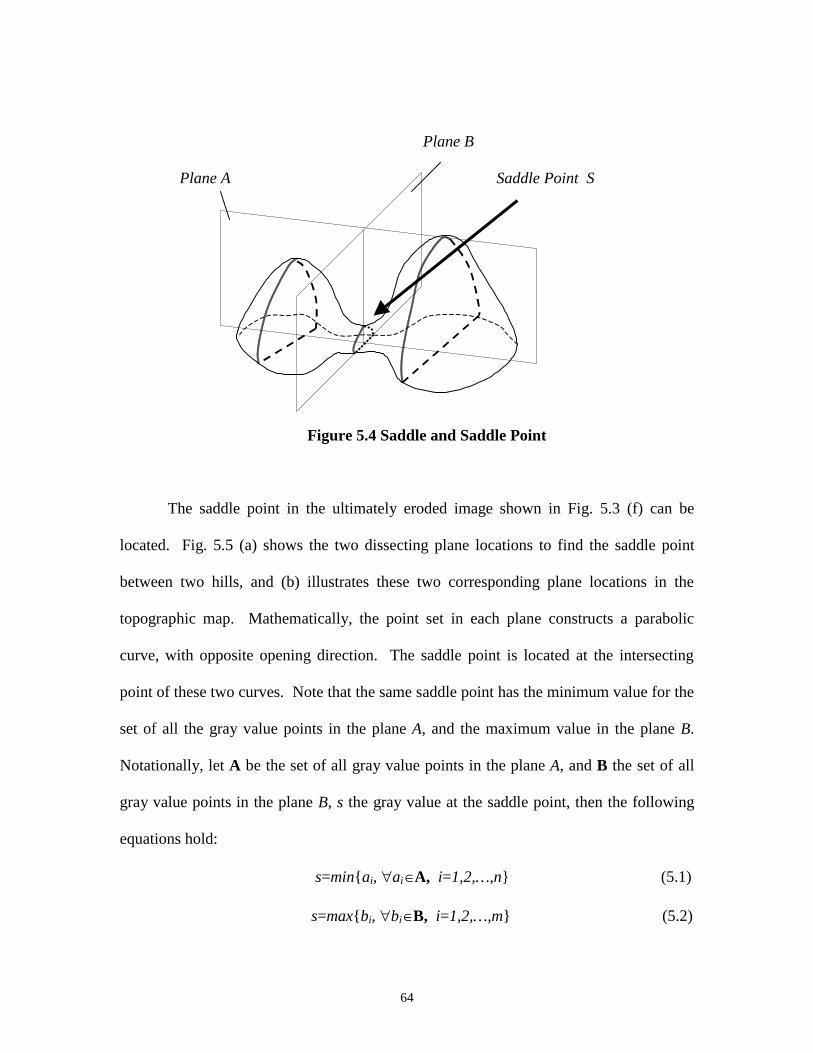
The saddle point in the ultimately eroded image shown in Fig. 5.3 (f) can be
located. Fig. 5.5 (a) shows the two dissecting plane locations to find the saddle point
between two hills, and (b) illustrates these two corresponding plane locations in the
topographic map. Mathematically, the point set in each plane constructs a parabolic
curve, with opposite opening direction. The saddle point is located at the intersecting
point of these two curves. Note that the same saddle point has the minimum value for the
set of all the gray value points in the plane A, and the maximum value in the plane B.
Notationally, let A be the set of all gray value points in the plane A, and B the set of all
gray value points in the plane B, s the gray value at the saddle point, then the following
equations hold:
s=min{ ai, �ai�A, i=1,2,…,n} (5.1)
s=max{ bi, �bi�B, i=1,2,…,m} (5.2)
65
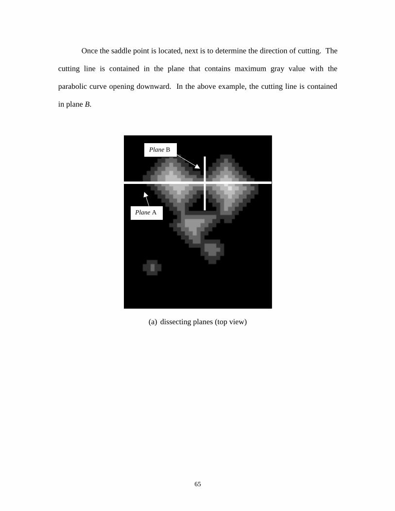
Once the saddle point is located, next is to determine the direction of cutting. The
cutting line is contained in the plane that contains maximum gray value with the
parabolic curve opening downward. In the above example, the cutting line is contained
in plane B.
(a) dissecting planes (top view)
Plane B
Plane A
66
(b) dissecting planes (oblique view)
Figure 5.5 Dissecting Planes for Finding Saddle Point
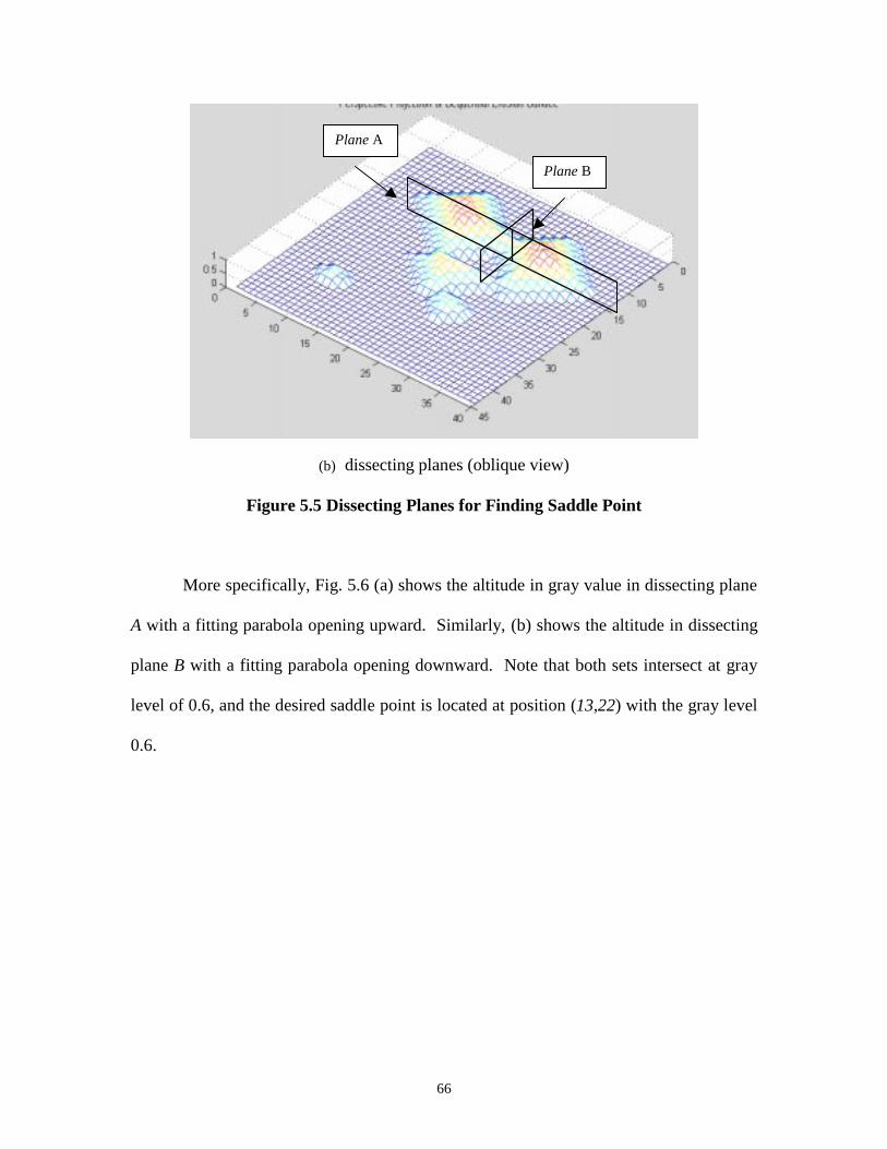
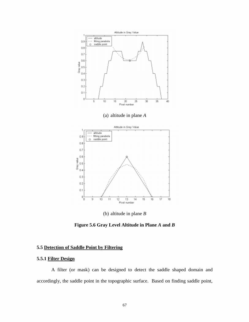
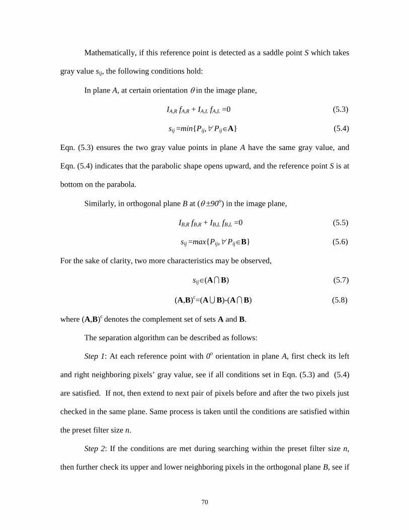
More specifically, Fig. 5.6 (a) shows the altitude in gray value in dissecting plane
A with a fitting parabola opening upward. Similarly, (b) shows the altitude in dissecting
plane B with a fitting parabola opening downward. Note that both sets intersect at gray
level of 0.6, and the desired saddle point is located at position (13,22) with the gray level
0.6.
Plane A
Plane B
67
(a) altitude in plane A
(b) altitude in plane B
Figure 5.6 Gray Level Altitude in Plane A and B
5.5 Detection of Saddle Point by Filtering
5.5.1 Filter Design
A filter (or mask) can be designed to detect the saddle shaped domain and
accordingly, the saddle point in the topographic surface. Based on finding saddle point,
68
the cutting line can be oriented and separation can be carried out. Since the geometric
characteristics of saddle surface are known, a filter was engineered to serve the separating
purpose.
Again, hold the same definitions made for the plane A, plane B and the set A, set
B, as stated in the last section. Further, let a filter have the size of n�m, each grid holds
value fij, i=1,2,…,n, j=1,2,…,m. Fig. 5.7 shows a filter of size 5�5.
Figure 5.7 A Filter of Size 5�5
The objective of designing a filter is to locate the saddle point. This requires that
the filter can detect the gray value points distributing in a parabolic pattern in both planes
A and B. To achieve this, the value in each grid of the filter is assigned with +1 or –1,
symmetric about the reference point fij in planes A and B. At each reference point, plane
A and B are assumed to be orthogonal to each other, and may rotate simultaneously from
0o to 90o anti-clockwise searching for the orientation that qualifies the reference point to
be the saddle point. If the preset conditions as given in the next section are met, the
current reference point becomes the saddle point, and cutting then begins in the
orientation of plane B. Fig. 5.8 demonstrates the values given for a filter of size 5�5, and
the filter rotates from 0o to 90o.
f11 f12 f13 f14 f15
f21 f22 f23 f24 f25
f31 f32 f33 f34 f35
f41 f42 f43 f44 f45
f51 f52 f53 f54 f55
69
(a) filter at 0o (b) filter rotated by 22.5o
(c) filter rotated by 45o (d) filter rotated by 67.5o (e) filter rotated by 90o
Figure 5.8 Rotation of Filter
5.5.2 Saddle Point Conditions
The filter demonstrated above can be extended to any larger size, and the rotating
angle step then may be smaller accordingly. Suppose that in the plane A, there exist two
points that are symmetrical to the reference point S (recall that S is also in the plane B).
Let these two points denote PA,R and PA,L (subscript R and L indicate Right and Left to S in
the plane A), which take the gray value (altitude) IA,R and IA,L, respectively.
Correspondingly, assume that the filter values at these two locations are fA,R and fA,L (Note
that if one is +1, the other must be –1), respectively.
0 0 +1 0 0
0 0 +1 0 0
+1 +1 0 -1 -1
0 0 -1 0 0
0 0 -1 0 0
0 +1 0 0 0
0 +1 0 -1 -1
0 0 0 0 0
+1 +1 0 -1 0
0 0 0 -1 0
+1 0 0 0 -1
0 +1 0 -1 0
0 0 0 0 0
0 +1 0 -1 0
+1 0 0 0 -1
0 0 0 -1 0
+1 +1 0 -1 0
0 0 0 0 0
0 +1 0 -1 -1
0 +1 0 0 0
0 0 -1 0 0
0 0 -1 0 0
+1 +1 0 -1 -1
0 0 +1 0 0
0 0 +1 0 0
70
Mathematically, if this reference point is detected as a saddle point S which takes
gray value sij, the following conditions hold:
In plane A, at certain orientation � in the image plane,
IA,R fA,R + IA,L fA,L =0 (5.3)
sij =min{ Pij,� Pij�A} (5.4)
Eqn. (5.3) ensures the two gray value points in plane A have the same gray value, and
Eqn. (5.4) indicates that the parabolic shape opens upward, and the reference point S is at
bottom on the parabola.
Similarly, in orthogonal plane B at (� �90o) in the image plane,
IB,R fB,R + IB,L fB,L =0 (5.5)
sij =max{ Pij,� Pij�B} (5.6)
For the sake of clarity, two more characteristics may be observed,
sij�(A� B) (5.7)
(A,B)c=(A � B)-(A� B) (5.8)
where (A,B)c denotes the complement set of sets A and B.
The separation algorithm can be described as follows:
Step 1: At each reference point with 0o orientation in plane A, first check its left
and right neighboring pixels’ gray value, see if all conditions set in Eqn. (5.3) and (5.4)
are satisfied. If not, then extend to next pair of pixels before and after the two pixels just
checked in the same plane. Same process is taken until the conditions are satisfied within
the preset filter size n.
Step 2: If the conditions are met during searching within the preset filter size n,
then further check its upper and lower neighboring pixels in the orthogonal plane B, see if
71
all conditions set in Eqn. (5.5) and (5.6) are satisfied. If not, check next pair of pixels’
gray value extending upward and downward within the preset filter size m.
Step 3: If an affirmative answer has been obtained for step 1 and 2, in other
words, if logical AND is used to combine the two conditions set in step 1and step 2, and a
positive answer is found, then the current reference point is the desired saddle point.
Followed is to carry out the cutting process in the direction of plane B. Step 1 to Step 3
are repeated for the next new reference point in the image.
Step 4: If a negative answer has been found in either step 1 or step 2, in other
words, the AND logic fails, then the current reference point is not the saddle point at the
current orientation, stop.
Step 5: Simultaneously rotate the plane A and plane B to certain orientation, repeat
step1 to step 5.
Step 6: If after a rotation of 90o is finished, and no AND logic is found affirmative,
then the current reference point is detected as a non-saddle-point. Move to the next new
reference point, repeat Step 1 to Step 6.
The simplified pseudocode of separation for touching and overlapping shapes is
listed as follows:
72
Table 5.2 Pseudocode of Separation
/*A gray scale ultimately eroded image G is available, and a filter of size n�m is selected.*//*Scan with the filter */for (each reference point)
if (within the filter size n in plane A, all conditions are met, referring to Eqn. (5.3)and (5.4)) AND (within the filter size m in plane B, all conditions are met, referring to Eqn. (5.5) and (5.6)) - the current reference point is a saddle point - cut in the direction of plane B else
- simultaneously rotate both plane A and B anti-clockwise to certain angle, provided a total 90o isnot swept. Otherwise stop.
- go back to above ”if ” condition, check AND logic again in new orientation just rotated. end
end /* end of “for” loop */
Referring to Fig. 5.5 (a), the separated shapes are shown in Fig. 5.9 (b), while (a)
shows the connected shapes.
(a) connected shapes (b) separated shapes
Figure 5.9 Separation by Filtering
5.6 Testing on a Real Image
Now, using a structuring element of size 3�3 for sequential erosion, and a filter of
size 15�15 for saddle point detection, the touching and overlapping limestone rocks
73
digitized in a 484�512 matrix, as shown in Fig. 5.10 (a), was separated. The
corresponding binary image is given in sub-figure (b). A total of 10 erosion operations
has been elapsed before the ultimate erosion is reached. Sub-figure (c) demonstrates the
resultant topographic surface, while (d) portraits the same topographic surface in an
oblique view. Finally, an image of separated particles is presented in sub-figure (e).
(a) gray scale image
74
(b) binary image
(c) topographic surface (Top view)
75
(d) topographic surface (Oblique view)
76
(e) particle separated image
Figure 5.10 Separation Process
The size of the filter used in the separation process is problem dependent. Larger
filters give more accurate detection, but take longer to perform the filtering. Proper size
can be determined experimentally. Some “false cutting” can occur for particles whose
edge contour is significantly concave on opposite edges.
77
6. VOLUMETRIC MODELING
6.1 Introduction
Particle size distribution (gradation) in the Superpave and in many other
applications is based on the sieve mesh sizes and particle mass. In most sieving
operations, gradation is evaluated as “percent-passing” by mass. The minor diameter of
the particle profile shape obtained through using principal eigen analysis is used as a
particle’s size. This dimension is correlated to the sieve size. In this research, the density
is assumed a constant, so the total mass is proportional to the volume of aggregates. Also
in this research, all the obtainable information comes from a 2-D image. Volume
information is not directly observed. Lack of 3-D information brings the need to estimate
the volume using some of the available 2-D measurements, such as area, aspect ratio,
signature mean and variance. In other words, modeling the volume of aggregates is
needed.
Statistical techniques are important for image analysis. From the images captured
of the mineral aggregates, all the sizes and shapes are random. The process of extracting
useful information becomes equivalent to estimating random variables. The objective in
this chapter is to estimate the volume of mineral aggregates to serve the purpose of
gradation.
6.2 Modeling Sample Preparation
To observe how particle mass might be correlated with some of its parameters
found in 2-D images, some samples of aggregate were collected. Fig. 6.1 demonstrates
images of some of these samples. Altogether 501 pieces of limestone rock varying in
78
size and shape were imaged. The following measurements were taken for each individual
particle:
� Projected area (mm2)
� Major and minor diameter (mm)
� Aspect ratio
� Non-normalized signature mean (mm) and variance (mm2)
� Mass (g) and volume (mm3) with a measured constant density of of 0.00305
(g/mm3)
The methods for obtaining above measurements except mass and volume were
described in Chapter 4. The mass of each particle was found using a laboratory digital
balance, and added to the data vector. All the measurements are listed in Appendix I.
The aggregates were arranged on the lighting box as shown in Fig. 6.1 so that each
particle could be paired with its image statistics. The particles’ sizes are visually judged
ranging from 4.75 (mm) to 25.00 (mm).
(a) size � 4.75 (mm) (b) size � 9.50 (mm)
79
(c) size � 12.50 (mm) (d) size � 19.00~25.00 (mm)
Figure 6.1 Sample Photos
To gain some intuitive perceptions about how some parameters from a particle’s
2-D image influence its mass, Fig. 6.2 illustrates the observations in which the mass of
each individual particle is plotted against its area, aspect ratio, non-normalized signature
mean and variance, major and minor diameter, respectively.
(a) mass vs. area (b) mass vs. aspect ratio
80
(c) mass vs. signature mean (d) mass vs. signature variance
(e) mass vs. major diameter (f) mass vs. minor diameter
Figure 6.2 Sample Data Observations
If coupled with shape information, the particle’s projected area can reflect its size.
The signature mean is basically the “effective radius”. The projected area and signature
mean are apparently the dominant factors that correlate with the mass from both intuitive
and experimental considerations. The general trend shows that particle mass value grows
as its area and signature mean increase. The aspect ratio gives partial information about
the profile shape, but is obviously not correlated directly with mass, at least in this
81
sample. The signature variance may reveal how irregular the particle shape is, more
specifically, how far the actual edge line deviates from the circumference whose radius
is the signature mean. Major and minor diameter also indicate particle size.
Evidently, discovering a way to more accurately predict particle’s 3-D
measurements should be attempted based on combinations of several pertinent 2-D
variables. The objective here must be to create a model using appropriate measurements
from the image data, so that a “good” model is obtained. A good model will be the one
in which the estimated particle volumes and the actual particle volumes are equal, at least
when averaged over sufficient number of particles.
6.3 Model Selection
Regression analysis is a statistical technique for modeling the relationship
between two or more variables. Once an adequately good model is found, it is then used
to predict the response to the new set of variables of the same type. In fact, multiple
regression is one of the most widely used statistical techniques [16].
In general, for a dependent variable, or response, y that may be related to k
independent variables, the standard multiple linear regression (MLR) model takes form
����� ������ kk xxxy ...22110 (6.1)
where
y : Observation or response.
�j : Partial regression coefficient, j=0,1, 2, …k
xj : Regressor variable, j=1, 2, …k
�: Random error with zero mean and variance �2.
82
This model describes a hyperplane in the k-dimensional space of the independent
variables {xj}. The parameter �j represents the expected change in the response y per unit
change in xj when all the remaining independent variables xi (i�j) are held constant.
It is worth mentioning that, in general, any regression model that is linear in the
parameters, that is, the � values, is a linear regression model. Models that are polynomial
or include interaction effects in the parameters may also be analyzed by multiple linear
regression model by defining regressor variables that include the nonlinear effects [16].
In matrix notation, the model in Eqn. (6.1) can be expressed as
Y=X�+� (6.2)
Where
Y=
����
����
�
ny
y
y
�
2
1
X=
������
������
�
nknn
k
k
k
xxx
xxx
xxx
xxx
�
����
�
�
�
11
33231
22221
11211
1
1
1
1
�=
����
����
�
k�
�
�
�
2
1
�=
����
����
�
n�
�
�
�
2
1
The summation of error square is
��
�n
iiL
1
2� =�T �=(Y-X�)T(Y-X�) (6.3)
83
The vector of least square estimators, �
â , can be obtained by minimizing L and satisfying
��
�
ââL
= -2XTY+2XTX�
â =0 (6.4)
thus
�
â =(XTX)-1XTY (6.5)
The estimated regression model is
��
� âXY (6.6)
6.4 Particle Geometric Assumptions and Definitions
To use MLR model, the regressor variables that may influence the observations
must be found. Reasonably, these variables are particle geometry related.
Referring to Fig. 6.3, some important variables that will relate to the prospective
MLR model are defined:
Htop : Top height, which is measured from the imaged background up to the
highest point found in the upper surface of the particle.
Hcent : Central height, which is also measured from the imaged background and
through the centroid of the profile shape to the upper surface.
Hnom : Nominal height, which is the most related variable. The value of this
height quantitatively results from the actual volume of the particle, as
illustrated in sub-figure (a), divided by its projected area, as depicted in
sub-figure (c). In other words, the actual volume of any particle can be
obtained by multiplying its projected area with its nominal height.
Dmaj : Major diameter of the particle’s profile shape.
84
Dmin : Minor diameter of the particle’s profile shape.
Viewing direction
Htop Hcent
(a) actual shape and volume
Hnom
(b) equivalent shape and volume Dmaj
Dmin
(c) common projected area
Figure 6.3 Geometric Perspective of Particle
85
It is clear that the posture of the particles in the imaging scene may affect the
modeling results. Here the following assumptions regarding the pattern of particle
positioning in the imaged scene are claimed:
1) After randomly vibrating and toppling, the majority of the particles will lie on
the background with their maximum projected area facing down. This state is
termed “stable state” hereafter.
2) All particles are assumed to have a constant density.
The assumption 1) can lead to the following inequalities:
For any geometric objects, at the stable state
0<Hnom�Hcent�Htop�Dmin (6.7)
While for the most crushed limestone aggregates at the stable state, it holds
0<Hnom�Dmin (6.8)
thus
10min
��D
H nom (6.9)
The term
minD
Hnom is defined as the flatness of particle throughout this work.
6.5 MRL Model Building
Flatness of the particle is suspected to relate to some geometric attributes, such as
elongation, roundness of the profile shape, and jaggedness of the edge line. All the
mentioned variables are defined to be particle size and volume independent.
86
Following MLR model is build first, then each variable in it is described
thereafter.
����� ���
�
�
��
�
�
���
����
������
�1
23min
2min
10min
log2 sig
sig
sig
majnom
M
V
M
D
D
D
D
H (6.10)
where
Hnom : Nominal height (mm).
Dmin : Minor diameter (mm).
Dmaj : Major diameter (mm), also as defined in Chapter 4.
Msig : Mean value of the non-normalized signature (mm).
Vsig : Variance of the non-normalized signature (mm2).
� : Random error.
Definition and interpretation of each variable in Eqn. (6.10) are as follows:
minD
Hnom : Flatness, as illustrated in Fig. 6.4 (a).
minD
Dmaj : Elongation. It takes the value of aspect ratio, as depicted in Fig. 6.4 (b).
sigM
D
2min : Roundness. It measures the circularity of the particle. Its value increases
to 1 as the profile shape of the particle becomes more circular. See Fig.
6.4 (c).
2sig
sig
M
V : Jaggedness. For a perfectly smooth edge line, the value is zero, as
demonstrated in Fig. 6.4 (d).
87
Dmin Dmin
Dmaj
Hnom
Dmaj
(a) flatness: minD
Hnom (b) elongation: minD
Dmaj
2Msig Msig
Vsig
Dmin
(c) roundness: sigM
D
2min (d) jaggedness:
2sig
sig
M
V
Figure 6.4 Interpretation of Model Variables
Some aspects regarding 2sig
sig
M
V need to be mentioned here: first, the signature
mean is squared in the denominator to make the parameter dimensionless. Second, the
logarithm transformation of 2sig
sig
M
V makes the very small ratio values more readable and
offsets the possible inaccuracy caused by numerical truncation in the computer system.
Third, the reciprocity of the negative logarithm transformation ensures a positive value
that decreases to zero as the edge line becomes smoother. To clearly demonstrate the
88
purpose of this data transformation, given a array of small (not very small in order to
view the plots effectively) values, starting from 0.01 up to 0.33, increasing step by 0.04,
Fig. 6.5 shows values of the logarithm transformation of this array, and the final values of
the negative reciprocity of this transformation.
Figure 6.5 Data Transformation
The model in Eqn. (6.10) can be simplified, correspondingly, as
Yflat = �0+�1Xelong+�2Xround+�3Xjagged+� (6.11)
where Xelong , Xround, and Xjagged are equivalent to the corresponding regressor variables in
Eqn. (6.10).
In matrix notation,
Yflat=�
â X+� (6.12)
The unbiased regression coefficient estimators are thus in matrix form
�
â =(XTX)-1XTYflat (6.13)
89
The prediction of flatness for each particle is
jaggedroundelongflat XXXY 3210
�����
���� ���� (6.14)
where
minD
HY
nomflat
�
�
� (6.15)
Recall that the final goal is to use this model to predict the volume of the particle.
Since the volume estimate used in this research equals the projected area multiplied by
corresponding nominal height, the following expression holds:
partflatpartnom ADYAHV min
���
�� (6.16)
where
Apart : Particle projected area (mm2).
6.6 Overall Modeling Effect
Using all the available data from the modeling sample of 501 particles, the
complete model in Eqn. (6.10) was found to be:
1
2min
minmin
log4668.02
4754.01390.06660.0
��
��
�
�
��
�
�
���
����
������
sig
sig
sig
majnom
M
V
M
D
D
D
D
H (6.17)
From Eqn. (6.14) and Eqn. (6.15), Eqn. (6.16) can be rewritten as
To simplify the statistical analysis of the model, Eqn. (6.19) is treated as an
approximated standard MLR model with zero intercept. A number of techniques can be
used to measure the adequacy of a multiple regressor model [16]. Two of those
techniques to present the adequacy of the model were used. The pertinent theoretical
basis can be reviewed in the book by Hines and Montgomery [16] and Myens [18].
6.7.1 The Coefficient of Multiple Determination
The coefficient of multiple determination, in a loose sense, is a measure of the
amount of reduction in the variability of the response obtained by using the regressor
93
variables [16], is defined in the problem as
vv
E
S
SSR ��12 (6.20)
where
��
�
�
���
��� ���
501
1
2n
iii
TE VVSS åå (6.21)
n
V
VViS
n
ii
Tn
i
ivv
2501
12501
1
��
���
�
����
��� ��
��
�
�
�
�
�
-VV (6.22)
where SSE is the sum of squares for error, and Svv is the sum of squares.
For the modeling sample of 501 particles, it was calculated that SSE= 118075237,
Svv= 1257933386, thus R2=0.91. This indicates that about 91% of the variability in the
actual volume V has been explained when the three regressor variables are used in the
model.
6.7.2 Error Normality
One of the assumptions for fitting a regression model is that the errors are
uncorrelated random variables and normally distributed with mean zero and constant
variance, i.e., NID(0, 2e� ). Fig. 6.8 shows the errors plotted against the particle
sequence. Note that it follows the same particle sequence as that used in Fig. 6.6.
94
Figure 6.8 Model Error vs. Particle Sequence
To test the normality of the residual which is the difference between actual
volume and estimated volume, one may standardize the residuals by computing the
quantity
E
ii
MSd
�� (6.23)
where i=1,2,3,…, n
MSE : mean squares, and
2)( eEMSE �� (6.24)
where E(�) denotes the expectation, and 2e� is the error variance [16].
95
If the error are NID(0, 2e� ), then approximately 95% of the standardized residuals
should fall in the interval (-2,2). Fig. 6.9 presents the histogram of the dI’s for the
sample.
Figure 6.9 Histogram of Standardized Residuals
The percentage of the resultant standardized residuals that are within (-2,2) is
found to be 94.01 %, the errors can thus be regarded as being distributed normally.
6.8 Model Testing
The quality of the developed volumetric model needs to be tested using the
randomly selected samples. If the sample population satisfies the size range (minor
diameter is between 4.75 mm and 25.00 mm), it is reasonable to expect a satisfactorily
accurate result.
96
6.8.1 Preparation of Testing Sample Population
Due mainly to the size constraints of the lighting box on which the particles are
placed, the number of particles in an image is limited. Eight batches of testing sample
were prepared. Particles in each batch were then placed in the imaging scene and were
photographed. The same particles were photographed five times. Each time the particles
were “stirred up” to give a completely new image. The five images of each batch were
marked with a, b, c, d, e respectively for analysis, thus there were 40 total images in the
sample.
To test the model, one out of five images from each sample batch was randomly
selected. The statistics of the each batch are tabulated in Table 6.1. The histograms of
some useful measurements for each and for the combined batch are included in Appendix
II. The total actual mass of the each batch is obtained by weighing.
Table 6.1 Sample Measurement Statistics
Batch /Image
#
Totalparticle
#
Totaltrue
mass (g)
Areamean(mm2)
AreaSTD+
(mm2)
Majordiameter
mean(mm)
MajorDiameter
STD+
(mm)
Minordiameter
mean(mm)
MinorDiameter
STD+
(mm)
#1 / b
#2 /a
#3 / e
#4 / d
#5 / a
#6 / a
#7 / c
#8 / e
345
376
215
251
378
76
71
150
316.25
265.91
475.06
383.46
625.52
512.02
521.38
1006.19
96.3661
75.2003
169.2037
125.3001
128.0232
362.9582
376.1573
356.2143
40.0473
38.4560
81.5658
75.1036
78.6642
197.1795
204.8211
206.9573
11.4350
9.8945
15.4329
13.1246
13.1727
23.5464
23.1580
22.5798
3.0401
3.4555
4.7307
4.4820
5.0281
7.7220
7.3076
8.0629
7.8602
6.5525
10.8713
8.8168
8.8973
16.1730
17.3936
16.2522
2.2699
2.1892
3.6119
3.6209
5.9956
5.3785
6.2691
6.1154
STD+ : Standard deviation.
97
6.8.2 Testing Results
For five images from the same batch, eight batches in total, using the volumetric
model and the same density used before to compute the estimated mass, sub-figure (a)
shows the estimated mass of each image from batch #1 to #8. So, for a single batch,
every five mass estimates are plotted versus one actual mass. In (b), for each batch,
averaging these five estimated mass values as a data point, then plot them against the
actual mass. (c) demonstrates the percent error from (b).
(a) mass comparison
98
(b) mass comparison
(c) percent error
Figure 6.10 Model Testing for Mass
99
From sub-figure (c), it is observed that the percent error can reach as high as
around �6% for batch #4, #5and #6. If the size of the population N is increased, the
accuracy can then be improved. To do this, take a random combination of the images,
and each image of the combination was randomly selected from one of the eight batches.
This indicates that the total number of particles will increase up to N=1862, which is a
total particle number of eight batches. Fig. 6.11 illustrates such a random combination
formed by image b,a,d,e,c,e,c,d from the sample batch #1, #2, … #8, respectively.
100
Figure 6.11 A Random Combination of Sample Batches (badececd)
Batch #2 (N2 =376 particles)
Photo a
Photo b
Photo c
Photo d
Photo e
Batch #3 (N3 =215 particles)
Photo a
Photo b
Photo c
Photo d
Photo e
Batch #4 (N4 =251 particles)
Photo a
Photo b
Photo c
Photo d
Photo e
Batch #5 (N5 =378 particles)
Photo a
Photo b
Photo c
Photo d
Photo e
Batch #6 (N6 =76 particles)
Photo a
Photo b
Photo c
Photo d
Photo e
Batch #7 (N7 =71 particles)
Photo a
Photo b
Photo c
Photo d
Photo e
Batch #8 (N8 =150 particles)
Photo a
Photo b
Photo c
Photo d
Photo e
Photo a
Photo d
Photo e
Photo c
Photo e
Photo c
Photo d
Combination
Photo b
Batch #1 (N1 =345 particles)
Photo a
Photo b
Photo c
Photo d
Photo e
N=1862
101
100 combinations were tested. Each combination may represent one “grand”
image covering all 1862 particles. Each new constituent image results from a new “stir-
up”, and in total 100 stir-ups were conducted for producing 100 grand images. The result
is shown in Fig. 6.12. Fig. 6.13 shows the percent error,which mainly stays within �2%,
and is greatly reduced as anticipated.
Figure 6.12 Modeling Result for 100 Combinations
102
Figure 6.13 Percent Error for 100 Combinations
103
7. SIEVING CORRELATION
7.1 Introduction
Since the Superpave specifications are given on the basis of percent passing by
mass, two correlations must be made. First, particles are optically sieved into “bins” or
sizes based on the minor dimension of the particle. In each bin, the number of particles is
not important, rather, the total mass of the particles in that bin is. Second, particle’s
mechanical sieving behavor must be correlated with the optical sieving behavor. The
model which correlates information obtained from the 2-D image to the volume has been
established. In this chapter, a sieving correlation method was developed by first
modeling the particle cross section into a rectangle, plus the scaling factors obtained from
calibration to take the actual cross section shape and other related elements into account.
Based on the flatness distribution from 501 sample particles, a criterion was set to
determine the sieving strategy for each particle. Results are presented as gradation curves
in the format used for Superpave analysis. The optical sieving results were also
compared against mechanically sieved measurements of the same samples to test
accuracy. The results showing satisfactory correspondance were presented.
7.2 Identified Sieving Problems
Either a circular sieve opening or a cylindrical particle as shown in Fig. 7.1 (a)
will make the sieving process easy to describe analytically. In either case, the fashion in
which the particles fall through the sieve opening is rotation invariant in the falling
direction. Unfortunately, neither the sieve opening shape nor the cross section of the
particle is circular. Sieve openings are square, and the cross section of crushed particles
104
is randomly shaped as illustrated in Fig. 7.1 (b). This makes the sieving analysis rather
complex.
Cross section
Profile shape
(a) circular cross section (b) random shape cross section
Figure 7.1 Particle Cross Section Shape
For example, for a fairly flat particle with 22 mm minor diameter, it is clear that it
can not pass if its minor diameter is parallel to the square sieve opening of 19.00 mm.
However, after rotating a certain angle � , it becomes passable since 22 mm is smaller
than the diagonal (26.87 mm) of the square opening, as shown in Fig.7.2. There is a
tendency for flat particles, especially those with rounded edges to pass diagonally
through the sieve.
105
22 mm
Cross section Sieve opening Passable
Particle �
Profile shape
Impassable 19.00 mmDirection of passing
Figure 7.2 Particle Passing Mechanism
In vision sieving, the particle minor diameter is approximately known, but particle
thickness is not, and the thickness is undoubtedly a critical factor that influences particle
sieving behavior. This requires development a method for relating the 2-D observable
features to the sieving behavior of particles. It will probably be impossible to do this
with extreme accuracy for individual particles. However, it is expected that reasonably
accurate results for bulk measurements should be obtained.
7.3 Analytical Discussion
To simplify the complexity of the sieving behavior problem, the interaction
between the particle cross section and the square mesh of a given sieve was first
analytically modeled. Let dsv be the size of a given sieve, and as defined previously,
Dmin be the minor diameter, and Hnom be the nominal height. This way the cross section
takes the shape of a rectangle, as illustrated in Fig. 7.3.
106
Actual cross section contour
Hnom
Dmin
Figure 7.3 Modeled Particle Cross Section
The interaction of the cross section with the sieve size takes place only for those
particles whose minor diameters are within the range dsv<Dmin< 2 dsv. The reason that
the equal sign “=” was not included is that, if particle minor diameter equals the sieve
size, it is expected to pass, while if it has the same dimension as the diagonal of square
mesh, it will be retained with certainty, since particles are not “razor thin”.
Given a sieve mesh size dsv, the critical position for a particle with assumed
rectangular cross section of minor diameter Dmin and nominal height Hnom to pass or be
retained in the sieve is illustrated in Fig. 7.4.
107
Hnom
Dmin Hcrit
Actual cross section
45o
dsv
Figure 7.4 Critical Position
For any given minor diameter Dmin satisfying dsv<Dmin< 2 dsv., it has a “critical
height”, denoted as Hcrit in above figure. The hatched rectangle is correspondingly
formed by Dmin and Hcrit , as also shown in above figure. If the nominal height Hnom is
shorter than Hcrit , the particle passes this sieve, otherwise it is retained. The following
simple relation holds for Hcrit and Dmin :
min2 DdH svcrit �� (7.1)
108
Two special cases determine the range of Hcrit
i) if Dmin= 2 dsv , then Hcrit =0. This means that unless the particle is “razor
thin”, it will be retained on the sieve. Particles with this Dmin will always be
retained in practice.
ii) if Dmin= dsv , then Hcrit =0.4142 Dmin. Particles with this Dmin will be expected
to pass the sieve.
From i) and ii), the range of the critical height is thus
0<Hcrit<0.4142 Dmin (7.2)
Recall that the flatness of the particle is defined as
minD
HY nom
flat � (7.3)
and further define the critical flatness for a particle of Dmin as
minD
HY crit
crit � (7.4)
Apparently, the state of any particle of Dmin in the sieve can be determined by the
following conditions:
���
�
�
retainedYYif
passYYif
critflat
critflat
,:
,: (7.5)
One may argue that for the crushed limestone aggregates, the shapes of the cross
section are not retangular, so the conditions set in inequality (7.4) are not sufficient to
determine a particle’s passing or being retained. To remedy this, a calibration factor is
obtained experimentally and added to correct the above conditions, as described later .
109
7.4 Sieving Probability Analysis
For any particle with Dmin in a sieve, the conditions expressed in inequality (7.5)
are fundamental for judging its ultimate state: passing or being retained. From Eqn. (7.1)
and (7.4), the corresponding critical flatness can thus be easily obtained as
12min
��D
dY sv
crit (7.6)
Now the question arises: what is the flatness, Yflat, of the particle of interest?
The sample of 501 particles was analyzed to determine the probability distribution
of the particle flatness. Fig. 7.5 and Fig. 7.6 present a scatter diagram and a histogram of
the sample flatness statistics.
Figure 7.5 Scatter Diagram of Sample Flatness
110
Figure 7.6 Sample Flatness Histogram
The cumulative distribution of the 501 sample particles is obtained from the
probability density data. Its approximated distribution function is attained by applying a
curve-fitting technique, shows as the solid curve in Fig. 7.7. The distribution function is
approximated as
P(Ycrit)=-19.9524 5critY +67.4.1075 4
critY -83.6898 3critY +44.4792 2
critY -7.6510 critY +0.4069
(7.7)
111
Figure 7.7 Sample Flatness Distribution
The strategy for using the function in Eqn. (7.7) is straightforward:
1) Given the particle’s measured minor diameter Dmin, select those particles for
which dsv<Dmin< 2 dsv .
2) Calculate the Hcrit.
3) From the cumulative probability distribution function in Eqn. (7.7), calculate
P*={P(Yflat)�Ycrit} (7.8)
where P(�) indicates probability.
4) Create a random number � on [0,1] using a uniform distribution.
5) If �� P*, the particle passes. Otherwise it is retained.
112
This approach makes no attempt to determine analytically whether an individual
particle passes or is retained. Rather, it exploits the central tendency of the data to
provide an estimate which proves to be fairly accurate over a large sample.
For the sake of convenience, rewrite inequality (7.5) which are the conditions for
sieving behavior.
���
�
�
retainedYYif
passYYif
critflat
critflat
,:
,: (7.9)
Recall that inequalities expressed in (7.9) are based on the assumption that the
particle has rectangle shaped cross section which is not true in reality. Also, the
conditions in (7.9) is for analytical determination whether an individual particle passes or
is retained. At this point, the analytical determination for an individual partilcal has been
converted to statistical determination for a group of particles. This fact imposes an
additional modification to P* to compensate for inaccuracies caused by irregular shaped
cross section. Referring to the steps in using sample flatness distribution function stated
previously, multiply P* by a scaling factor called sieving calibration factor, �sv , where
�sv �1.00. Then conditions for sieving behavior becomes
���
�
�
retainedPif
passPif
sv
sv
,:
,:*
*
��
�� (7.10)
where �sv can be calibrated experimentally for the given sieve size.
7.5 Sieving Phase Analysis
7.5.1 Size Modification for Triangular Shapes
The minor diameter of the shape is regarded as the size that determines the
sieving behavior. For triangular shaped particles as shown in Fig. 7.8, however, the
113
actual sieve size will be greater than the minor diameter, to an extent that may vary
according to the actual shape. This requires to sort out those triangle shapes, and modify
the minor diameter that is the most vital element to determine passing or staying on a
given sieve.
Figure 7.8 Triangle Shaped Particles
Rather than determine the modifying extent for each triangular particle, the minor
diameter is multiplied by a correction factor, which can be obtained experimentally. This
factor found to work well is:
)1(min*min �� DD (7.11)
where
*minD : modified minor diameter.
� : a uniformly distributed random number within [0,0.3].
114
7.5.2 Sieve Series and Sieving Phase
The same sample population that had been applied to test the volumetric model
was used to determine the calibration factors, �sv . As stated previously, it consists of
eight batches, whose basic statistics are tabulated in Table 6.1. The histograms of some
measurements for each batch and for the total sample are included in Appendix II.
The sieve set consists of five sizes: 4.75 mm, 9.50 mm, 12.50 mm, 19.00 mm, and
25.00 mm. They are stacked with the largest mesh size at the top, with successively
smaller mesh sizes below, as shown in Fig. 7.9. For the sake of notational convenience,
dsv denotes a sieve of any size. Note that the particles in investigation are poured in the
top 25.00 mm sieve, falling through onto the next sieve below if not retained. Sieves are
vibrated and rotated using an automatic sieve shaker.
115
Particles
dsv25.00 =25.00 mm
dsv19.00 =19.00 mm
dsv12.50 =12.50 mm
dsv9.50 =9.50 mm
dsv4.75 =4.75 mm
Figure 7.9 Physical Sieve Cascade
For a given sieve of size dsv, only those particles whose minor diameter Dmin, are
within the range dsv <Dmin< 2 dsv, are candidates for sieving behavior consideration.
The particles outside this range will be either retained in the upper sieve or pass through
onto the lower sieve.
Fig. 7.10 outlines the overall sieving analysis for the whole prospective sample
population.
116
: A symbolic curve that means the particle may or may not be retained on the
sieve.
: The state in which all particles within the corresponding size range are
partially retained, i.e., some pass, some remain in the current sieve.
: The state in which all particles within the corresponding size range are
absolutely retained.
: The state in which all particles within the corresponding size range are
partially retained either in the sieve of dsv12.50, or in the sieve of dsv9.50.
Retained probability1.00
0.00 dsv2.36 dsv4.75 dsv9.50 dsv19.00
dsv12.50
4.75 2 4.75 9.50 12.50 2 9.50 2 12.50 19.00 25.00
Overall Particle size (mm)
Figure 7.10 Overview of Sieving Phase Analysis
After all particles in the image scene have been processed, three available
parameters can be used to conduct the vision sieving process: shape, minor diameter, and
estimated mass, denoted as Sshp, Dmin, and �
M , respectively. For N particles in the image
117
scene having been processed, a data array can thus be formed ready for vision sieving
processing:
�
�
�
�
�
�
�
��
�
�
NNNshp
NNNshp
shp
shp
MDS
MDS
MDS
MDS
min,,
11min,1,
12min,2,
11min,1,
��� (7.12)
The shape parameter gives information about the triangle shaped particles, whose
minor diameter must be modified to correctly relate them to their sieving behavior.
In the algorithm, the sieving starts off with scanning the first column in matrix
(7.12), finding triangles and modifying their diameters. Then the second column is
scanned to group particles by size into bins for the percent passing statistics. The
elements in the third column are assigned to the corresponding “volume bins” (sieves)
suitable to their minor diameters. At the end of the “binning ” algorithm, the percent
passing is computed as the Superpave specifies according to the formula:
100
1
1 �
�
�
�
�
�
�
N
w
w
m
k
k
M
M (7.13)
where
m : the total number of particles retained in the sieve in question.
N : the total number of particles in the population.
118
kM�
: mass of kth particle in the sieve in question.
wM�
: mass of wth particle in the population.
The pseudocode of the overall sieving procedure is given in Table 7.1. Note that
the actual working code can be written in various ways, and the coding presented in the
following pseudo code is not necessarily the optimal one. The major purpose here is to
clearly present the logic thread imbedded in the optical sieving phase.
119
Table 7.1 Pseudocode of Sieving Procedure
/* After all particles have been processed, and the matrix of (7.12) is formed */
/* Scan 1st column for triangular shapes. */for (each shape element in 1st column)
if (it is a triangle) - modify its minor diameter in the 2nd column. endend
/* Scan 2nd column for excluding particle sizes that are definitely retained in the sieve. */for (each minor diameter element in 2nd column)
if (Dmin� 4.75 or 4.75 2 �Dmin� 9.50 or 12.50 2 �Dmin� 19.00 )- place its mass into the corresponding sieve that retains it.
endend
/* Scan 2nd column again for particle sizes that are partially retained in the sieve. */for (each minor diameter element in 2nd column)
if (Dmin� 19.00 or 9.50 2 �Dmin� 12.50 2 or 12.50�Dmin� 9.50 2 or …
9.50�Dmin� 12.50 or 4.75�Dmin� 4.75 2 , referring to Fig. 7.10 )- compute for its critical flatness Ycrit using Eqn. (7.6)- calculate the probability P(Yflat)�Ycrit using Eqn. (7.7)- generate a uniformly distributed random number � .
if (� � )( critsv YP� , referring to conditions in (7.10) )
- pass the current sieve.
if (12.50�Dmin� 9.50 2 ) - place it into sieve 9.50 mm for testing again. end /* end of “if” condition * /
elseif (� > )( critsv YP� , also referring to conditions in (7.10)
- retained in the current sieve. Place its mass in this sieve. end /* end of “if” condition * /
end /* end of “if” condition * /
end /* end of “for” loop * /
/* Compute for the percent passing using Eqn (7.13) * /
7.6 Benchmark
The particle size distribution (gradation) obtained from the vision sieving is
calibrated against the results obtained from mechanically sieving the same sample. The
120
result works as the “benchmark” for the sieving parameter calibration. The same eight
batches of sample particles were used to obtain the benchmark.
The eight batches of sample particles are mechanically sieved. Each batch was
sieved ten times in order to achieve better accuracy. As a result, for each batch, ten
percent passing curves and ten percent retained curves were obtained. The desired
results, the percent retained and percent passing, can be acquired. By percent retained, it
means the percent of the particles in terms of volume (or mass) retained on each of the
five sieves. As an example, Fig. 7.11 (a) and (b) shows the result for batch #4 of percent
retained and percent passing from mechanical sieving, respectively.
(a) percent retained
121
(b) percent passing
Figure 7.11 Percent Retained and Percent Passing for Sample Batch #4
As expected, each resultant curve does not coincide with each other. In other
words, ten times of mechanical sieving come up with ten different results. Two major
reasons may explain these differences. First, borderline particles may only pass for a
very particular orientation, which may or may not be achieved during the random
tumbling of the sieving process. Secondly, attrition occurs during the sieving process.
When all the particles are toppling in the enclosure of the vibrating and rotating sieves,
particles are hitting and breaking down each other, inevitably reducing the size and
volume of each particle. As a consequence, the mass in each sieve decreases as sieving
goes on. This affects the value of percent retained, and thereby, affects the percent
passing. Fig. 7.12 shows for sample batch #7 the data scattering for the 9.50 mm, 12.50
mm, and 19.00 mm sieve results.
122
Figure 7.12 Mass Change in Sieving Process
To obtain the benchmark, the data points at each sieve size was averaged. Fig.
7.13 (a) (b) shows the benchmark of percent retained and percent passing, respectively,
for sample batch #4.
123
(a) percent retained (b) percent passing
Figure 7.13 Benchmark for Sample Batch #4
By the same method, the benchmark of all other batches was obtained, and given
in Appendix III.
A sample population of larger size was formed by combining all the particles
from the eight batches The corresponding percent retained and percent passing
benchmark are shown in Fig. 7.14, and the values are listed in Table 7.2.
7.7 Sieving Calibration Factor
Using a large sample population formed by combining all eight batches, the
sieving calibration factor, �sv, as introduced in inequality (7.10), was calibrated to be
�sv=
�
�
�
�
�
�
�
�
�
00.1
00.3
00.7
00.2
75.4
950
1250
00.19
�
�
�
�
(7.14)
The calibration factors can be interpreted as follows:
The cross section of the particle is not rectangular. In most cases, the height at
two ends of the minor diameter is shorter than the critical height Hcrit, as illustrated
124
previously in Fig. 7.4. This apparently increases the probability for the particles to pass
the sieve. �sv�1 accounts for this rounding effect.
For each sieve of different size, there is a different calibration factor value. All
these factors have been determined by back calculation from the large sample population
with known size distribution. With the addition of these calibration factors, the sieving
strategy’s conditions expressed in inequality (7.10) becomes semi-empirical, because
they are empirically derived values. The significance of �sv is that it accounts for
numerous effects such as particle’s cross section shape distribution. In summary, the
physical significance is to account for combination of the following aspects:
1) The effect of the particle’s cross section shape distribution. Although there is
no theoretical a priori knowledge about cross section shape distribution
inherent in the used method, it does affect the behavior of particles in the
sieve to pass or be retained.
2) The effects of separation of overlapping and touching particles. Using the
developed algorithm, the separated particles’ shape and mass are not the same
as they are manually isolated. This affects the particle’s sieving behavior.
Again, no a priori knowledge is available to determine even statistically how
the sieving behavior will be influenced.
3) The effects caused by vision system errors such as hardware calibration,
software imperfection.
4) The effects of sample population size.
125
(a) percent retained (b) percent passing
Figure 7.14 Benchmark for Combined Sample Batches
Table 7.2 Benchmark Values for Combined Sample Batches
Sieve Size (mm)Type
4.75 9.50 12.50 19.00 25.00
PercentRetained (%)
28.806 23.996 28.390 18.250 0.000
PercentPassing (%)
0.557 29.383 53.385 81.766 100
7.8 Vision Sieving Result
With the calibrated �sv’s, sieving correlation testing conducted. The samples are
the same as those used for volumetric model testing, i.e., eight batches with a total of
1862 particles. Recall that the benchmark has been available, as shown in Fig. 7.14. The
basic algorithm was written in Table 7.1
Again, a random combination of the images was taken, each of combination’s
constituent image was randomly selected from one different sample batch. This indicates
that the total number of particles will increase up to N= N1+N2+…+N8 =1862, which is a
126
summation of particle number of all eight batches. Fig. 7.15 illustrates how a random
combination of photo d, a, b, e, b, d, c, a selected from sample batch #1, #2, …, #8
respectively, is formed.
127
Figure 7.15 A Random Combination of Sample Batches (dabebdca)
Batch #1 (N1 =345 particles)
Photo a
Photo b
Photo c
Photo d
Photo e
Batch #2 (N2 =376 particles)
Photo a
Photo b
Photo c
Photo d
Photo e
Batch #3 (N3 =215 particles)
Photo a
Photo b
Photo c
Photo d
Photo e
Batch #4 (N4 =251 particles)
Photo a
Photo b
Photo c
Photo d
Photo e
Batch #5 (N5 =378 particles)
Photo a
Photo b
Photo c
Photo d
Photo e
Batch #6 (N6 =76 particles)
Photo a
Photo b
Photo c
Photo d
Photo e
Batch #7 (N7 =71 particles)
Photo a
Photo b
Photo c
Photo d
Photo e
Batch #8 (N8 =150 particles)
Photo a
Photo b
Photo c
Photo d
Photo e
Photo a
Photo b
Photo e
Photo b
Photo d
Photo c
Photo a
Combination
Photo d
N=1862
128
In effect, each random combination represents one “grand” image covering all
1862 particles. Each constituent image results from a new “shuffling” of the same
sample batch. Therefore, each random combination of images may be regarded as result
of “grand shuffling” of 1862 particles.
Testing on five grand images was conducted. This means that 1862 particles were
shuffled five times to produce these five grand images. On each grand image, all
particles were “optically” sieve ten times, final vision sieving result is taken by averaging
these ten results, and then compare it to the benchmark.
Figures from Fig. 7.16 to Fig. 7.20 demonstrate the results of these five testings.
From the results, it shows that the percent passing residuals are within �3%. The residual
between the percent passing benchmark and vision sieving percent passing is listed in
Table 7.3. The error may be contributed to by the following reasons:
1) Simple measurement of the particle minor diameter is not an entirely true
representation of what happens in physical sieving. Particles that are
somewhat flat can turn diagonally in the sieve and pass a smaller mesh size
than one would suspect from simple size measurements.
2) Error in the calibration factor mm/pixel can contribute to vision sieving error.
3) Accurate measurement of percent passing requires accurate projection of the
volume from the optically measured parameters. This in practice is
impossible to achieve with extreme accuracy, especially for individual
particles.
4) Error existing in minor diameter estimation for triangular shapes can
contribute to sieving correlation error.
129
5) Overlapping and touching particles’ profile shape and volume estimate change
during separation.
6) If the size sample population is not sufficiently large, it will create error in
vision sieving process because a uniformly distributed random number is
involved in determining “pass or retain” for a particle in the sieve.
7) The benchmark itself has certain discrepancies due to particle physical sieving
behavior.
130
sieve size (mm) sieve size (mm)
(a) percent retianed (b) percent passing residual
(c) cumulative percent passing
Figure 7.16 Sieving Correlation Testing #1
(Combination: image e,e,d,b,c,d,c,e from sample batch #1 to #8, respectively)
131
sieve size (mm) sieve size (mm)
(a) percent retained (b) percent passing residual
(c) cumulative percent passsing
Figure 7.17 Sieving Correlation Testing #2
(Combination: image c,e,a,c,a,b,d,e from sample batch #1 to #8, respectively)
132
sieve size (mm) sieve size (mm)
(a) percent retained (b) percent passing residual
(c) cumulative percent passsing
Figure 7.18 Sieving Correlation Testing #3
(Combination: image e,d,e,a,a,a,b,c from sample batch #1 to #8, respectively)
133
sieve size (mm) sieve size (mm)
(a) percent retained (b) percent passing residual
(c) cumulative percent passsing
Figure 7.19 Sieving Correlation Testing #4
(Combination: image b,e,c,e,a,e,e,e from sample batch #1 to #8, respectively)
134
sieve size (mm) sieve size (mm)
(a) percent retained (b) percent passing residual
(c) cumulative percent passsing
Figure 7.20 Sieving Correlation Testing #5
(Combination: image e,d,d,a,c,e,d,b from sample batch #1 to #8, respectively)
37. N. H. Mearz, and W. Zhou, “Flat and Elongated: Advances Using Digital Image
Analysis.” Proceedings of the 7th Annual ICAR Symposium, International Center for
Aggregates Research, University of Texas at Austin, April19-21, 1999.
38. N. H. Mearz, “Online Fragmentation Analysis: Achievements in the Mining
Industry.” Proceedings of the 7th Annual ICAR Symposium, International Center for
Aggregates Research, University of Texas at Austin, April19-21, 1999.
39. A. Rauch, C. Hass, and H. Kim, “State of the Art in Aggregate Classification.”
Proceedings of the 7th Annual ICAR Symposium, International Center for Aggregates
Research, University of Texas at Austin, April 19-21, 1999.
40. T. C. Palangio, and N. H. Maerz, “Case Studies Using the Wipfrag Image Analysis
System.” FRAGBLAST 6th International Symposium for Rock Fragmentation By
Blasting, Johannesburg, South Africa, August 8-12, 1999, pp. 117-120.
41. B. M. K. Bocoum, “Hatch Sieving of Cylindrical Particles Cascadography.”
(master’s thesis, West Virginia University, n.d.).
154
APPENDIX I
Modeling Sample Statistics(Total of 501 particles)
Area : Projected area (mm2)Aps. : Aspect ratioDmaj : Major diameter (mm)Dmin : Minor diameter (mm)MNsig: Non-normalized signature mean (mm)VRsig : Non-normalized signature variance (mm2)Mass: Particle actual mass (g)