Page 1
Baw M.S. Thesis Presentation. Slide 1
Optical Interconnection Networks
Optical Interconnection NetworksDesign, Analysis, and Simulation Study of
M. S. Thesis Defense Presentationby
Ch’ng Shi Baw
Advisor: Prof. Mark A. Franklin
20 April 1999
Page 2
Baw M.S. Thesis Presentation. Slide 2
Optical Interconnection Networks
Presentation Organization
• Introduction– Background information & related work
• Thesis Contribution– Interconnection Network Simulator Framework
– Improving the Gemini interconnect architecture
• Conclusion– Summary and future work
Page 3
Baw M.S. Thesis Presentation. Slide 3
Optical Interconnection Networks
Thesis Contributions
• Interconnection Network Simulator (ICNS) framework– Design of the ICNS framework
– Simulator Verification
• Study of the Gemini network– Performance analysis
– Improving Gemini’s throughput
– Adding fair-scheduling capability to Gemini
Page 4
Baw M.S. Thesis Presentation. Slide 4
Optical Interconnection Networks
Introduction
• Interconnection network in generic terms
• Motivation: why optics
• Overview of enabling technologies
• The Gemini interconnect architecture and related works
• Simulation tool to aid design and study of interconnection networks
Page 5
Baw M.S. Thesis Presentation. Slide 5
Optical Interconnection Networks
Interconnection Network
• Terminals generate and/or consume data messages– e.g.: CPU, sensor banks, disks, other I/O devices
• Links and switches transport data
Page 6
Baw M.S. Thesis Presentation. Slide 6
Optical Interconnection Networks
Motivation
• Want to solve large problems fast.
• Target problems that are compute-, data-, and communications-intensive:– need multiple processors and high speed networks to
connect processors.
– want high bandwidth and low latency
• Use optics to build interconnection networks
Page 7
Baw M.S. Thesis Presentation. Slide 7
Optical Interconnection Networks
Motivation: Why Optics
• Strengths of optics:– very high bandwidth (tens of Tb/s in one fiber)
– low electro-magnetic interference
– virtually no transmission line effects at high speed
• Weaknesses of optics (current technology):– unsuitable to implement logical functions
– optical components are generally costly
Page 8
Baw M.S. Thesis Presentation. Slide 8
Optical Interconnection Networks
Optics: Technology Overview
• Guided-wave optics
• Free-space optics
• “Smart Pixel Array”
Arrays of VCSELs and detectors
Page 9
Baw M.S. Thesis Presentation. Slide 9
Optical Interconnection Networks
Optics: Technology Overview
• Free-space optics and “Smart Pixel Array”
– Potential to provide physically clutter-free interconnect
– Limited distance spanning capability
– Insufficient reliability study
Page 10
Baw M.S. Thesis Presentation. Slide 10
Optical Interconnection Networks
“Smart Pixel Array” ring architecture. [Chen98, Gourlay98, Lacroix98, Franklin]
Page 11
Baw M.S. Thesis Presentation. Slide 11
Optical Interconnection Networks
Optics: Technology Overview
• Guided-wave Optics– Fiber optics (mature, widely deployed)
– Polymer wave guides
• Recent developments:– polymer wave guides layout technology [Eldada96]
– efficient fiber-to-polymer wave guide coupling [Barry97]
– electro-optical switching elements [Sneh96, Lucent97]
Page 12
Baw M.S. Thesis Presentation. Slide 12
Optical Interconnection Networks
Electro-optical Switching
• The y-branch:
– Refraction index of LiNbO3 changes in the presense of electric field.
Page 13
Baw M.S. Thesis Presentation. Slide 13
Optical Interconnection Networks
Building on the y-branch
• A 2x2 electro-optical switch– Issues: power loss and crosstalk.
• Circuit-switched. No Buffering.
Page 14
Baw M.S. Thesis Presentation. Slide 14
Optical Interconnection Networks
Reducing Crosstalk
• Time-Dilation [Qiao96]– Reduce crosstalk using scheduling technique
• Space-Dilation– Add hardware
Page 15
Baw M.S. Thesis Presentation. Slide 15
Optical Interconnection Networks
– Space-dilation technique used by Lucent Technologies [Lucent97].
Next: Gemini Network Overview
Page 16
Baw M.S. Thesis Presentation. Slide 16
Optical Interconnection Networks
The Gemini Network• Use two networks
– one optically switched (Banyan topology to reduce power loss)
– one electronically switched
– as proposed, the two networks have identical topology [Chamberlain97]
• Main idea:– off-load bulk data to high-bandwidth optical network
– maintain low-latency in lightly-loaded electrical network to cater for control messages
• Goals (not related to performance):– easily manufacturable (low cost)
– forward compatibility
Page 17
Baw M.S. Thesis Presentation. Slide 17
Optical Interconnection Networks
The Gemini Network
Page 18
Baw M.S. Thesis Presentation. Slide 18
Optical Interconnection Networks
The Gemini Network
– Layout polymer wave guides using wire-printing techniques [Eldada96]
– Board level connection employs polymer-to-fiber coupling technique [Barry97]
– Assume space-dilation (use Lucent switch [Lucent97])
Page 19
Baw M.S. Thesis Presentation. Slide 19
Optical Interconnection Networks
Related Work
• Pan, Qiao, and Yang [Pan99]– Use 2x2 electro-optical switches
– Banyan topology
– Rely on time-dilation technique
Page 20
Baw M.S. Thesis Presentation. Slide 20
Optical Interconnection Networks
Time-Dilation
• Construct Contention-and-Conflict Free (CF) mappings– enforce switch element disjoint (SED) condition
– schedule connections so that no two connections share a switch element
• Assumes that a laser source can be completely turned off.
Page 21
Baw M.S. Thesis Presentation. Slide 21
Optical Interconnection Networks
• ExampleA set of CF-mappings for
a 4x4 network.
• Challenge is to find an optimal set of mappings for a given (arbitrary) set of connections
• Need 8 mappings for a 16 connections in a 4x4 network
• Need about 50 for 1000 connections (32x32 network)
• Polynomial time algorithm by Qiao to construct optimal set of CF-mappings [Qiao96]
• Assume the existence of a centralized controller
Next: The Need of a Simulation Tool
Page 22
Baw M.S. Thesis Presentation. Slide 22
Optical Interconnection Networks
Simulation Tool
• Simulation tools are generally helpful in the study of queueing systems
• Need an extensible simulator– vast interconnection network design space
– want the ability to easily extend simulator to simulate future optical network components
• Tune network design to specific applications– want the ability to incorporate application models into simulation
Next: Thesis Contribution
Page 23
Baw M.S. Thesis Presentation. Slide 23
Optical Interconnection Networks
Thesis Contributions
• Interconnection Network Simulator (ICNS) framework– Design of the ICNS framework
– Simulator and Simulation Verification
• Study of the Gemini network– Performance analysis
– Improving Gemini’s throughput
– Adding fair-scheduling capability to Gemini
Page 24
Baw M.S. Thesis Presentation. Slide 24
Optical Interconnection Networks
Interconnection Network Simulator(ICNS)
• Process-based discrete event simulation engine.• Object-oriented design.• Implementation environment:
– Uses the MODSIM III language developed by CACI Products Company.
– MODSIM III C++ executable.
– Simulation engine and MODSIM III to C++ compiler by CACI.
– C++ to executable compiler is gcc.
– Developed in Solaris 2.5 environment.
First Major Contribution of Thesis
Page 25
Baw M.S. Thesis Presentation. Slide 25
Optical Interconnection Networks
ICNS Framework: Base Classes
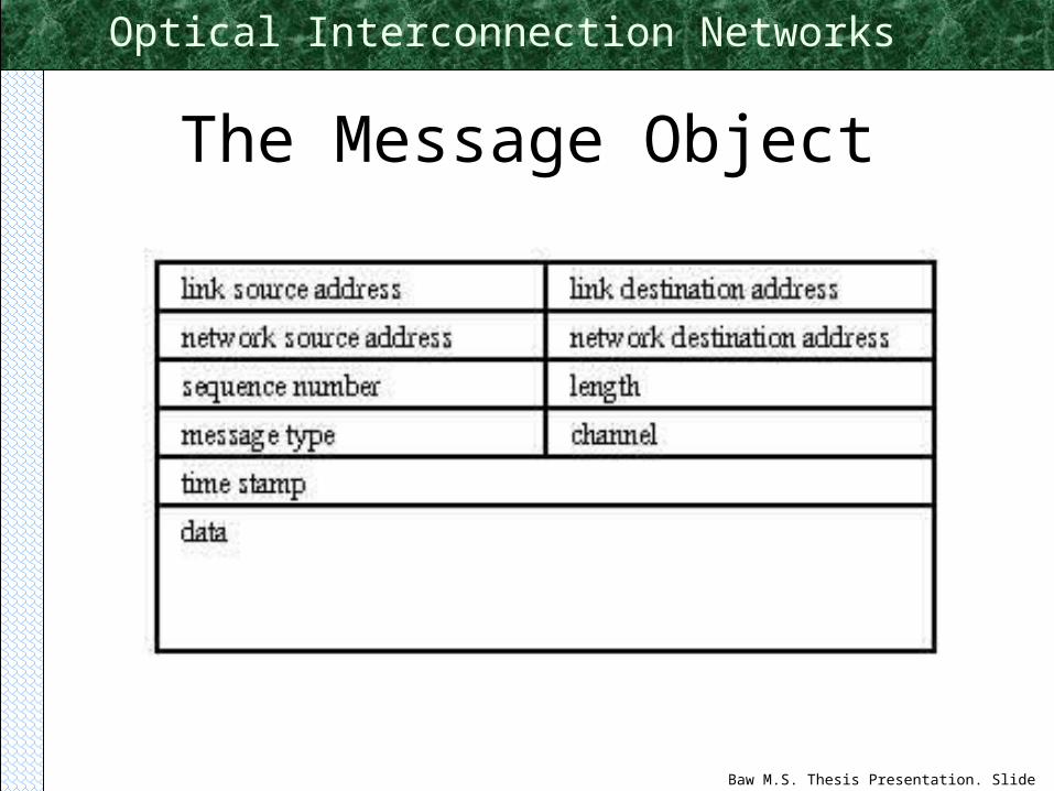
• MessageObj– models messages
– provides uniform interface to NodeObj
• NodeObj– abstract base class to be subclassed to model links, switches,
terminals, etc.
– provides uniform interface to MessageObj
• NetworkObj– container of NodeObj’s
– provide identifier-to-object-reference translation service
Page 26
Baw M.S. Thesis Presentation. Slide 26
Optical Interconnection Networks
ICNS Class Hierarchy
Page 27
Baw M.S. Thesis Presentation. Slide 27
Optical Interconnection Networks
Progression of a Simulation
• Interactions between MessageObj and NodeObj drive simulation forward.
• MessageObj’s operation:– Engaging a NodeObj:
• Ask if NodeObj is busy
• If it is, ask to be queued and terminate
• Ask to be processed otherwise
• Wait for the processing to finish (elapse simulation time)
• Terminate
Page 28
Baw M.S. Thesis Presentation. Slide 28
Optical Interconnection Networks
Progression of a Simulation
• NodeObj’s operations:– When asked if it is busy:
• answer yes or no
– When asked to queue a MessageObj• action depends on queueing policy (subclass-specific)
– When asked to process a MessageObj• action depends on which object is being simulated (subclass-specific)
• tell MessageObj how long to wait
Page 29
Baw M.S. Thesis Presentation. Slide 29
Optical Interconnection Networks
Description of Selected Objects
• Message• Link• Terminal
– Message Generator
– Buffer
– Central Processing Unit (CPU)
• Switch
Page 30
Baw M.S. Thesis Presentation. Slide 30
Optical Interconnection Networks
The Message Object
Page 31
Baw M.S. Thesis Presentation. Slide 31
Optical Interconnection Networks
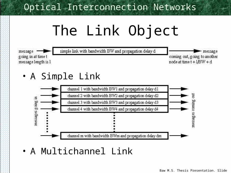
The Link Object
• A Simple Link
• A Multichannel Link
Page 32
Baw M.S. Thesis Presentation. Slide 32
Optical Interconnection Networks
The Terminal Object• Processing Node
Model
• Processing Node Model
Page 33
Baw M.S. Thesis Presentation. Slide 33
Optical Interconnection Networks
The Switch Object
• The 2x2 Switch Model
Page 34
Baw M.S. Thesis Presentation. Slide 34
Optical Interconnection Networks
An ICNS Application: sim• Separates topology from other network
parameters– Topology descriptor file (text file)
– Parameter descriptor file (text file)
• ParamObj– parses parameter descriptor file
– keeps track of all network parameters
• BuildGNetwork Procedure– procedure parses topology descriptor file, instantiates and
initializes objects accordingly
Page 35
Baw M.S. Thesis Presentation. Slide 35
Optical Interconnection Networks
sim: User Interface
• hand edit parameter file and topology file– or use Java-based GUI tools to generate files
• to invoke the sim program, typesim param_file topology_file
Page 36
Baw M.S. Thesis Presentation. Slide 36
Optical Interconnection Networks
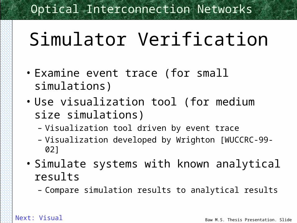
Simulator Verification
• Examine event trace (for small simulations)
• Use visualization tool (for medium size simulations)– Visualization tool driven by event trace
– Visualization developed by Wrighton [WUCCRC-99-02]
• Simulate systems with known analytical results– Compare simulation results to analytical results
Next: Visual Demonstration
Page 37
Baw M.S. Thesis Presentation. Slide 37
Optical Interconnection Networks
Visualization Tool Demo...
Page 38
Baw M.S. Thesis Presentation. Slide 38
Optical Interconnection Networks
M/M/1 and M/D/1 Simulations
• Verification Example:– Simulate parallel M/M/1 and M/D/1 systems
Page 39
Baw M.S. Thesis Presentation. Slide 39
Optical Interconnection Networks
M/M/1 and M/D/1 Simulations
• Within 3% of analytical results for loads up to about 92%
Page 40
Baw M.S. Thesis Presentation. Slide 40
Optical Interconnection Networks
Simulation Verification
• Simulate for long enough time to get valid statistics
• Wait out transient states to get valid steady-state statistics
• Demonstrated that simulator produced valid results for a wide range of loads– within 3% of analytical results for loads up to 92%
Next: The Gemini Network
Page 41
Baw M.S. Thesis Presentation. Slide 41
Optical Interconnection Networks
The Gemini Network
• Architecture Overview– Network Model
– Terminal Model
– Switch Model
• Basic Protocol
• Performance Limits
• Simulation Results
• Improvements ...
[Chamberlain97]
Page 42
Baw M.S. Thesis Presentation. Slide 42
Optical Interconnection Networks
Gemini Architecture Overview
• Network Model– Banyan
topology
– Bufferless, optically circuit-switched network
– Buffered, electronically packet-switched network
Page 43
Baw M.S. Thesis Presentation. Slide 43
Optical Interconnection Networks
Gemini Architecture Overview
• Terminal Model– CPU module
models applications
– One pair of optical output port
– One pair of electrical output port
Page 44
Baw M.S. Thesis Presentation. Slide 44
Optical Interconnection Networks
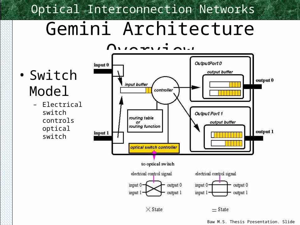
Gemini Architecture Overview
• Switch Model
– Electrical switch controls optical switch
Page 45
Baw M.S. Thesis Presentation. Slide 45
Optical Interconnection Networks
Gemini Network Protocol• Original Protocol
– Rely on Negative ACK
– Fire-on-timeout mechanism
– Issue:• How to set timeout parameter?
Page 46
Baw M.S. Thesis Presentation. Slide 46
Optical Interconnection Networks
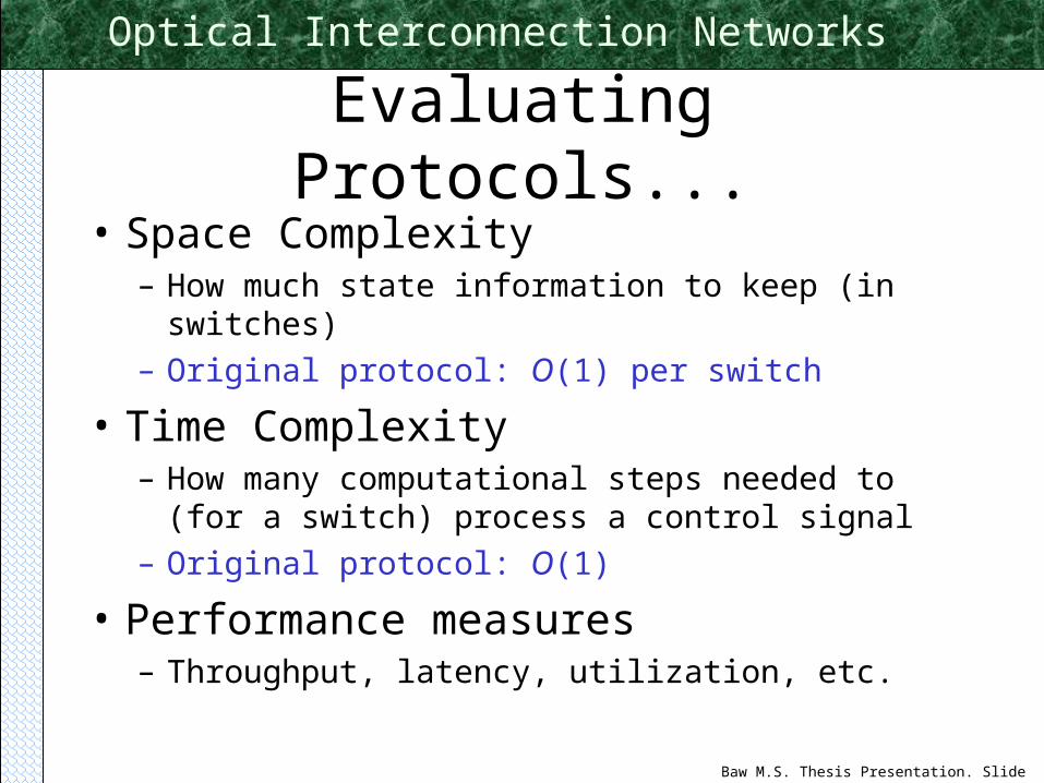
Evaluating Protocols...
• Space Complexity– How much state information to keep (in switches)
– Original protocol: O(1) per switch
• Time Complexity– How many computational steps needed to (for a switch)
process a control signal
– Original protocol: O(1)
• Performance measures– Throughput, latency, utilization, etc.
Page 47
Baw M.S. Thesis Presentation. Slide 47
Optical Interconnection Networks
The setup-teardown Protocol• Similar to original protocol
– But use positive ACK
– Fire upon ACK
• Signals– setup(S,D,blocked)
– ackSetup(S,D)
– block(S,D)
– teardown(S,D)
• Space Complexity O(1) per switch• Time Complexity O(1)
Page 48
Baw M.S. Thesis Presentation. Slide 48
Optical Interconnection Networks
Switch Operation• Each switch keeps a list and a one bit
optical switch state variable (= or x)
• Processing a setup(S,D,blocked) signal:– determine output port
– if setup already blocked, forward to output port.
– Determine requested state (= or x)
– if requested state conflict with current state and list is not empty• set blocked and forward to output port
– else set state to requested state, add S to list, forward to output port
• Processing a teardown(S,D) signal:– determine output port
– if S in list, remove S from list
– forward to output port
Page 49
Baw M.S. Thesis Presentation. Slide 49
Optical Interconnection Networks
Switch Operation Complexity
• Space Complexity O(1)– list size at most 2
• Time Complexity O(1)
Next: Performance Analysis
Page 50
Baw M.S. Thesis Presentation. Slide 50
Optical Interconnection Networks
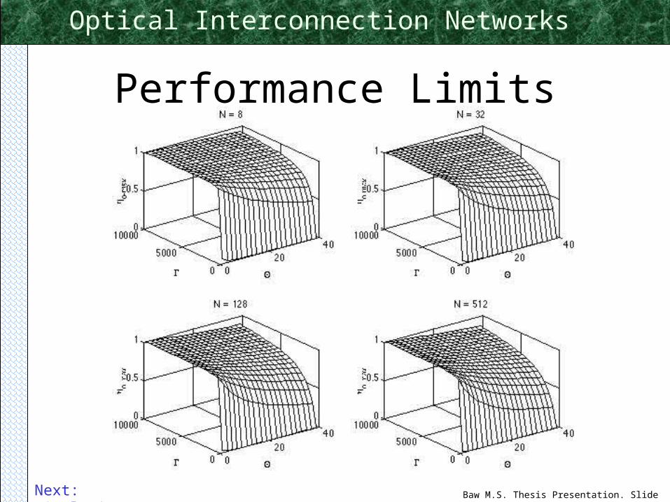
Performance Limits
• Optical network utilization efficiency limited by
• Define ,
Sendteardown
Sendsetup
… delay ... ReceiveackSetup
Send optical message
numerator
denominator
esigsigoo
ooo
BWlNBWl
BWl
/)3log)1(2(/
/
2
max
)3log)1(2( 2max
Nsig
o
sigo ll / eo BWBW /
Page 51
Baw M.S. Thesis Presentation. Slide 51
Optical Interconnection Networks
Performance Limits
Next: Simulations
Page 52
Baw M.S. Thesis Presentation. Slide 52
Optical Interconnection Networks
Performance Limits
Next: Simulations
Page 53
Baw M.S. Thesis Presentation. Slide 53
Optical Interconnection Networks
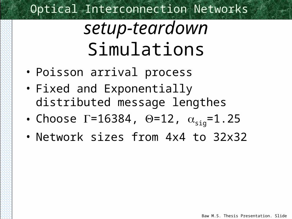
setup-teardown Simulations
• Poisson arrival process• Fixed and Exponentially distributed message
lengthes
• Choose =16384, =12, sig=1.25
• Network sizes from 4x4 to 32x32
Page 54
Baw M.S. Thesis Presentation. Slide 54
Optical Interconnection Networks
setup-teardown Simulation Results
Page 55
Baw M.S. Thesis Presentation. Slide 55
Optical Interconnection Networks
setup-teardown Simulation Results
Page 56
Baw M.S. Thesis Presentation. Slide 56
Optical Interconnection Networks
setup-teardown Simulation Results
Next: Blocking, the cause of low utilization
Page 57
Baw M.S. Thesis Presentation. Slide 57
Optical Interconnection Networks
Problem: Blocking
• Lose throughput due to blocking.
Page 58
Baw M.S. Thesis Presentation. Slide 58
Optical Interconnection Networks
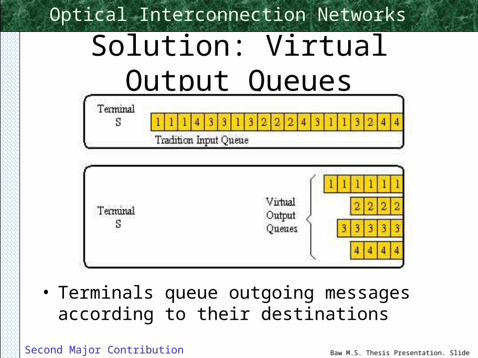
Solution: Virtual Output Queues
• Terminals queue outgoing messages according to their destinations
Second Major Contribution of Thesis
Page 59
Baw M.S. Thesis Presentation. Slide 59
Optical Interconnection Networks
VOQ Protocol
• Terminals allowed to send one setup request for each non-empty VOQ– Get around Head-of-Line blocking by exploring all possible optical
paths in parallel
• Switch processes setup, teardown signals as before– Add/delete source-destination pair to/from list instead
– Have N2 source-destination pairs
– but can bound list size to 2N
• Space Complexity O(N) per switch• Time Complexity O(1)
Page 60
Baw M.S. Thesis Presentation. Slide 60
Optical Interconnection Networks
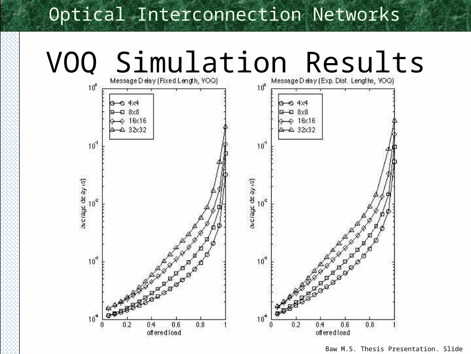
VOQ Simulation Results
Page 61
Baw M.S. Thesis Presentation. Slide 61
Optical Interconnection Networks
VOQ Simulation Results
Page 62
Baw M.S. Thesis Presentation. Slide 62
Optical Interconnection Networks
VOQ Simulation Results
Page 63
Baw M.S. Thesis Presentation. Slide 63
Optical Interconnection Networks
VOQ Simulation Results
Page 64
Baw M.S. Thesis Presentation. Slide 64
Optical Interconnection Networks
VOQ Simulation Results• Load on the electrical network
Network Size Load
4x4 < 0.6%
8x8 < 1.2%
16x16 < 2.4%
32x32 < 4.6%
• VOQ imposes minimal load on the electrical network– lightly loaded electrical network can maintain low latency for application
control messages
– variations of VOQ to further reduce electrical network load
Page 65
Baw M.S. Thesis Presentation. Slide 65
Optical Interconnection Networks
VOQ Complexity
• Even though there are N2 source-destination pairs, can implement list using bitmap and/or perfect hashing to make switch operations’ time complexities O(1).
• Space complexity is– N2 bits per switch if list is implemented as a bitmap
– 2N bits per switch if list is implemented using perfect hashing as well
• Can exploit regularity of Banyan network to construct simple perfect hash functions
Page 66
Baw M.S. Thesis Presentation. Slide 66
Optical Interconnection Networks
VOQ Implementation Complexity
Page 67
Baw M.S. Thesis Presentation. Slide 67
Optical Interconnection Networks
VOQ Merits and Demerits
• VOQ is good because:– VOQ significantly increases throughput
– VOQ adds only minimal complexity to the system
• But ...– VOQ may lead to starvation under very high load ...
Prevent starvation using fair scheduling techniques.
Next: Fair Scheduling in Gemini
Page 68
Baw M.S. Thesis Presentation. Slide 68
Optical Interconnection Networks
Fair Scheduling in Gemini• Starvation
– How and when it occurs
– what is the tradeoff
• Use fair scheduling to prevent starvation– concept of fairness in Gemini
• fairness granularity
• quantitative fairness measure
• Gemini fair scheduler design– what are the desirable characteristics
– the Distributed Deficit Round Robin (dDRR) fair scheduler
• Fair scheduler evaluation
Third Major Contribution of Thesis
Page 69
Baw M.S. Thesis Presentation. Slide 69
Optical Interconnection Networks
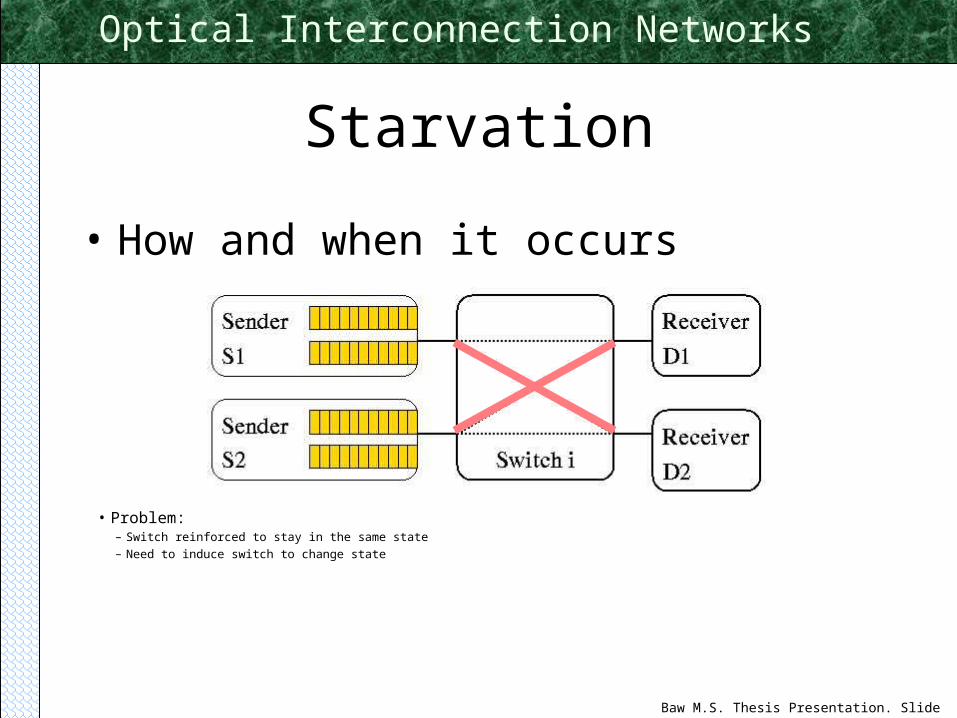
Starvation
• How and when it occurs
• Problem:– Switch reinforced to stay in the same state– Need to induce switch to change state
Page 70
Baw M.S. Thesis Presentation. Slide 70
Optical Interconnection Networks
Starvation: When does it occur?
• 4x4 network, 16 flows (i.e., source-destination pairs)
• Load is 0.8
• Plot cumulative number of bits sent versus flow number– snapshots taken at 500 and 20 message time intervals.
Page 71
Baw M.S. Thesis Presentation. Slide 71
Optical Interconnection Networks
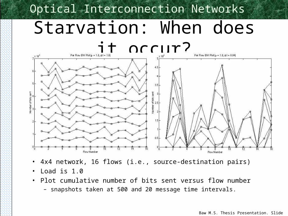
Starvation: When does it occur?
• 4x4 network, 16 flows (i.e., source-destination pairs)• Load is 1.0• Plot cumulative number of bits sent versus flow number
– snapshots taken at 500 and 20 message time intervals.
Page 72
Baw M.S. Thesis Presentation. Slide 72
Optical Interconnection Networks
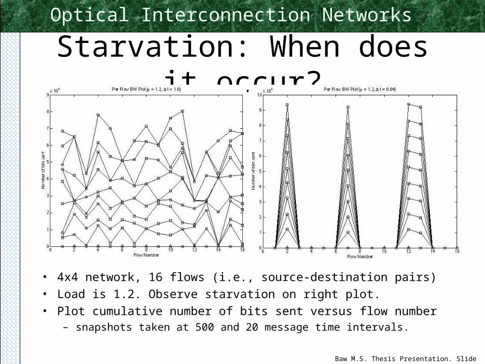
Starvation: When does it occur?
• 4x4 network, 16 flows (i.e., source-destination pairs)
• Load is 1.2. Observe starvation on right plot.
• Plot cumulative number of bits sent versus flow number– snapshots taken at 500 and 20 message time intervals.
Page 73
Baw M.S. Thesis Presentation. Slide 73
Optical Interconnection Networks
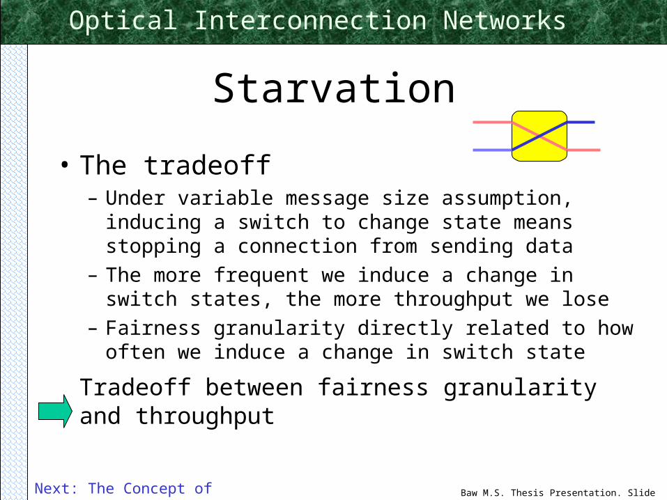
Starvation
• The tradeoff– Under variable message size assumption, inducing a
switch to change state means stopping a connection from sending data
– The more frequent we induce a change in switch states, the more throughput we lose
– Fairness granularity directly related to how often we induce a change in switch state
Tradeoff between fairness granularity and throughput
Next: The Concept of Fairness
Page 74
Baw M.S. Thesis Presentation. Slide 74
Optical Interconnection Networks
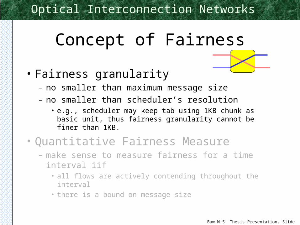
Concept of Fairness
• Fairness granularity– no smaller than maximum message size
– no smaller than scheduler’s resolution• e.g., scheduler may keep tab using 1KB chunk as basic unit,
thus fairness granularity cannot be finer than 1KB.
• Quantitative Fairness Measure– make sense to measure fairness for a time interval iif
• all flows are actively contending throughout the interval
• there is a bound on message size
Page 75
Baw M.S. Thesis Presentation. Slide 75
Optical Interconnection Networks
Fairness Measure
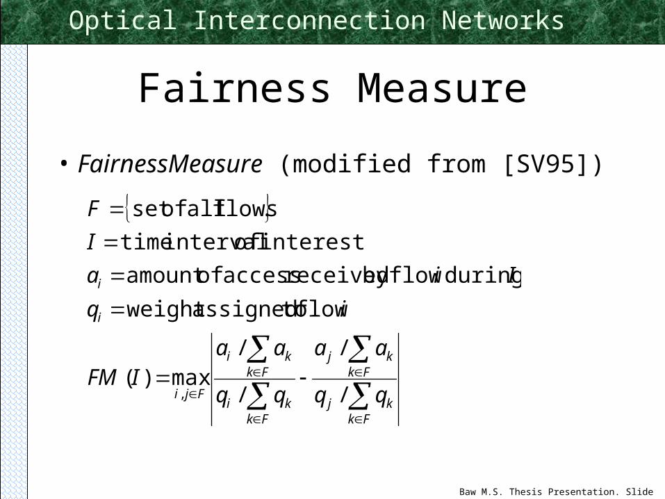
• FairnessMeasure (modified from [SV95])
Fkkj
Fkkj
Fkki
Fkki
Fji
i
i
qq
aa
qq
aaIFM
iq
Iia
I
F
/
/
/
/max)(
flow toassignedweight
during flowby received access ofamount
interest of interval time
.flows all ofset
,
Page 76
Baw M.S. Thesis Presentation. Slide 76
Optical Interconnection Networks
Fairness Measure
• Ideally fair system– FM(I) = 0 for all I
• Worst case– one flow monopolize access, all other flows starve
– FM(I) = |F|
• Worst case for Gemini– assume all connections actively contending for access
– FM(I) = N for an NxN network
Next: Scheduler Design Considerations
Page 77
Baw M.S. Thesis Presentation. Slide 77
Optical Interconnection Networks
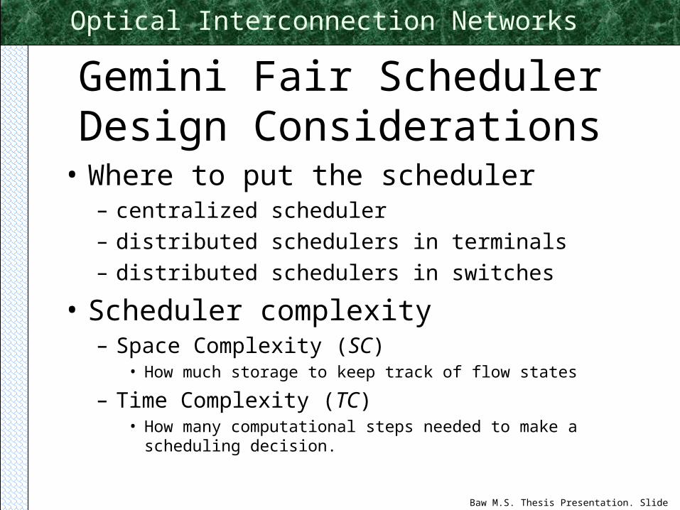
Gemini Fair SchedulerDesign Considerations
• Existing fair schedulers assume:– many-to-one contention: multiple flows contending for
one link (RR,WFQ,WF2Q,DRR,SCFQ,VCFQ,etc.)
– many-to-many contention, but in a non-blocking network (crossbar) [e.g., Prabhakar97, McKeown95]
– slotted time [Lu97, Prabhakar97, McKeown97]
– intermediate buffering available
• Gemini violates all the above assumptions.
Page 78
Baw M.S. Thesis Presentation. Slide 78
Optical Interconnection Networks
Gemini Fair SchedulerDesign Considerations
• Where to put the scheduler– centralized scheduler
– distributed schedulers in terminals
– distributed schedulers in switches
• Scheduler complexity– Space Complexity (SC)
• How much storage to keep track of flow states
– Time Complexity (TC)• How many computational steps needed to make a scheduling decision.
Page 79
Baw M.S. Thesis Presentation. Slide 79
Optical Interconnection Networks
Gemini Fair SchedulerDesign Considerations
• Desirable Characteristics– distributed in switches
– leverage underlying VOQ protocol
– low space and time complexities
– tunable fairness granularity (scheduler resolution)
• Modify DRR [SV95] to work in Gemini
Distributed DRR (dDRR)
Page 80
Baw M.S. Thesis Presentation. Slide 80
Optical Interconnection Networks
DRR Description• Scheduler resolution (fairness granularity)
determined by quota (quanta) assigned to flows• Keeps track of flow’s unused quotas
• dDRR uses similar ideas
Page 81
Baw M.S. Thesis Presentation. Slide 81
Optical Interconnection Networks
Switch to DRR slide show...
Page 82
Baw M.S. Thesis Presentation. Slide 82
Optical Interconnection Networks
dDRR Switch Controller Structure
• Each 2x2 electrical switch controller contains a partial dDRR scheduler.
• The dDRR module selectively blocks setup requests• Blocking is resolved by the VOQ module
Page 83
Baw M.S. Thesis Presentation. Slide 83
Optical Interconnection Networks
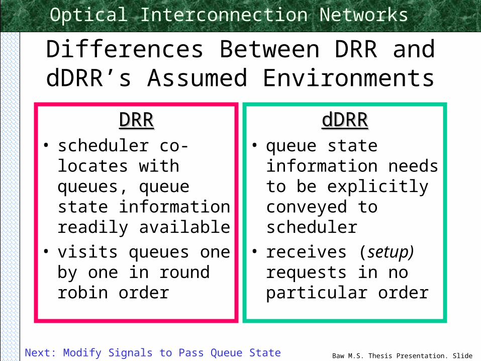
Differences Between DRR and dDRR’s Assumed Environments
DRRDRR• scheduler co-locates
with queues, queue state information readily available
• visits queues one by one in round robin order
dDRRdDRR• queue state
information needs to be explicitly conveyed to scheduler
• receives (setup) requests in no particular order
Next: Modify Signals to Pass Queue State Information
Page 84
Baw M.S. Thesis Presentation. Slide 84
Optical Interconnection Networks
Passing Queue and Flow State Information to dDRR Schedulers
VOQVOQ• setup(S,D,blocked)
• teardown(S,D)
dDRRdDRR• setup(flowID,blocked,amount)
• teardown(flowID,amount,more)
terminal-S
terminal-D
Next: dDRR Data Structure
Page 85
Baw M.S. Thesis Presentation. Slide 85
Optical Interconnection Networks
Switch to dDRR slide show...
Page 86
Baw M.S. Thesis Presentation. Slide 86
Optical Interconnection Networks
dDRR Data Structure in a Switch
qi dci spi nri morei qj dcj spj nrj morej qk dck spk nrk morek
q
dc
sp
nr
more
quantum is the amount by which a flow’s quota is replenished at each round
deficit counter keeps track of a flow’s available quota (initialized to q)
suspension flag indicates if a flow has exhausted its quota (initially set)
new round flag indicates if a flow has contended in the current round (initially set)
more flag indicates if a flow’s queue is empty (initially unset)
q dc sp nr more a dDRR entry for a flow
Next: dDRR Space Complexity
Page 87
Baw M.S. Thesis Presentation. Slide 87
Optical Interconnection Networks
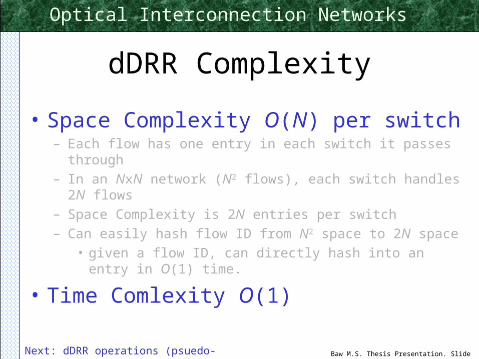
dDRR Complexity
• Space Complexity O(N) per switch– Each flow has one entry in each switch it passes through
– In an NxN network (N2 flows), each switch handles 2N flows
– Space Complexity is 2N entries per switch
– Can easily hash flow ID from N2 space to 2N space
• given a flow ID, can directly hash into an entry in O(1) time.
• Time Comlexity O(1)
Next: dDRR operations (psuedo-code)
Page 88
Baw M.S. Thesis Presentation. Slide 88
Optical Interconnection Networks
Processing a setup(i,amount) signal
module VOQ to),,( pass
unset
set
unset
else
set
set
if
elsif
set
if
blockedamountisetup
nr
more
sp
sp
blocked
qdcdc
nr
amountdc
blocked
nrsp
i
i
i
i
iii
i
i
ii
Next: Condition to set nri to be explained later
Page 89
Baw M.S. Thesis Presentation. Slide 89
Optical Interconnection Networks
Processing a teardown(i,amount,more) signal
module VOQ to),,( pass
set
else
if
moreamountiteardown
moremore
sp
qdc
amountdcdc
more
i
i
ii
ii
Note that the processing of setup and teardown signals is done in O(1) time.
Next: Determining Round Boundary
Page 90
Baw M.S. Thesis Presentation. Slide 90
Optical Interconnection Networks
Determine New Round Boundary
• A round ends if all flows have– either exhausted their quota
– or stopped contending (queues become empty)
• Begin a new round if all flows suspension flags become set
• Can check for New Round condition in O(1) time– test all suspension flags in parallel in hardware
Page 91
Baw M.S. Thesis Presentation. Slide 91
Optical Interconnection Networks
The New Round Operation
• Note that all operations take O(1) time• dDRR complexity for an NxN network:
– Space Complexity O(N) per switch
– Time Complexity O(1)
ii
i
moresp
nr
i
NewRound
set
floweach for
do Upon
Next: dDRR Feature and Functionality
Page 92
Baw M.S. Thesis Presentation. Slide 92
Optical Interconnection Networks
dDRR Feature and Functionality
• Properties inherited from DRR:– Tunable Fairness Granularity
• scheduler resolution determined by quanta assignment
• assign larger quanta to get coarser grained fairness– can trade off fairness granularity with throughput
– Weighted Fair Scheduling• assign different quanta to different flows to perform weighted
fair scheduling
• tradeoff not well understood
Next: dDRR Simulation Results
Page 93
Baw M.S. Thesis Presentation. Slide 93
Optical Interconnection Networks
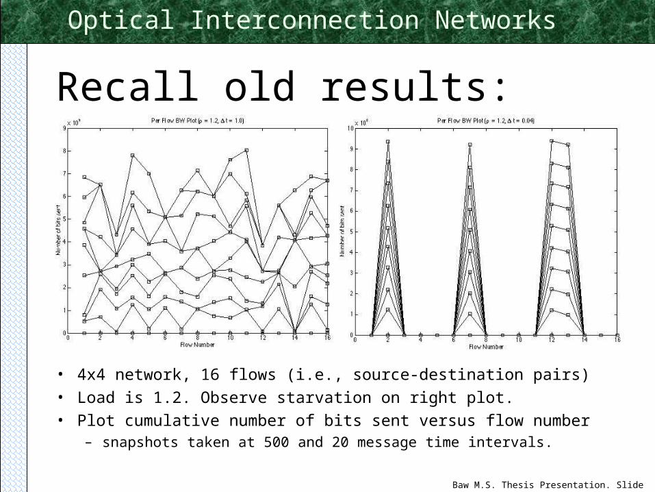
Recall old results:
• 4x4 network, 16 flows (i.e., source-destination pairs)
• Load is 1.2. Observe starvation on right plot.
• Plot cumulative number of bits sent versus flow number– snapshots taken at 500 and 20 message time intervals.
Page 94
Baw M.S. Thesis Presentation. Slide 94
Optical Interconnection Networks
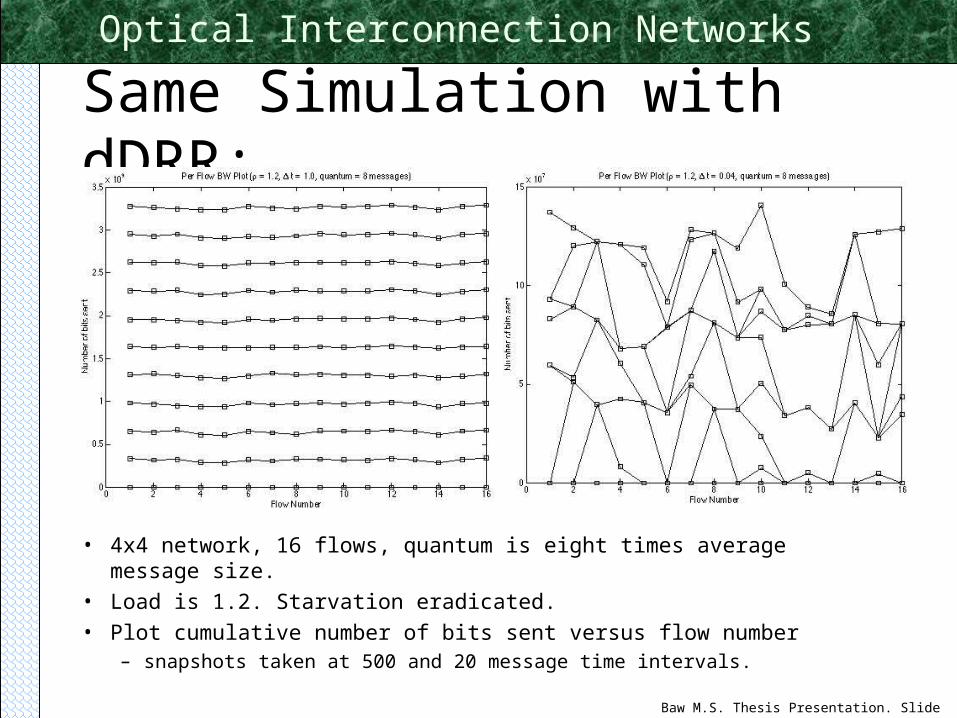
Same Simulation with dDRR:
• 4x4 network, 16 flows, quantum is eight times average message size.
• Load is 1.2. Starvation eradicated.
• Plot cumulative number of bits sent versus flow number– snapshots taken at 500 and 20 message time intervals.
Page 95
Baw M.S. Thesis Presentation. Slide 95
Optical Interconnection Networks
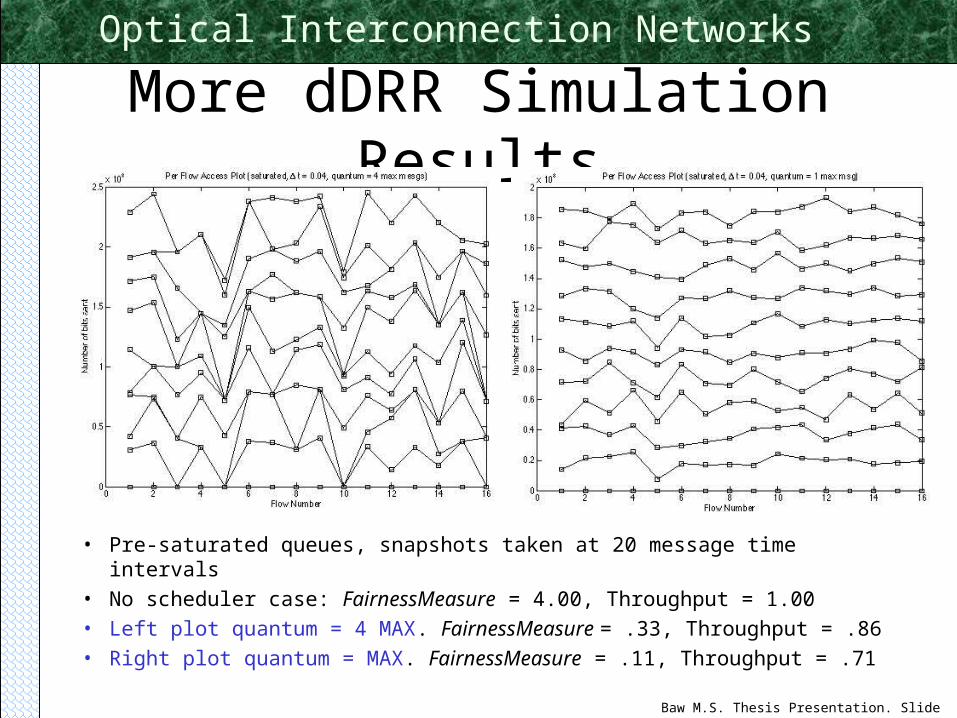
More dDRR Simulation Results
• Pre-saturated queues, snapshots taken at 20 message time intervals
• No scheduler case: FairnessMeasure = 4.00, Throughput = 1.00
• Left plot quantum = 4 MAX. FairnessMeasure = .33, Throughput = .86
• Right plot quantum = MAX. FairnessMeasure = .11, Throughput = .71
Page 96
Baw M.S. Thesis Presentation. Slide 96
Optical Interconnection Networks
Fairness Granularity vs. Throughput Tradeoff
• Pre-saturated queues, variable-size messages
• Plots of normalized throughput vs. quantum size (normalized to MAX)
Next: Weighted Fair Scheduling
Page 97
Baw M.S. Thesis Presentation. Slide 97
Optical Interconnection Networks
Fairness Granularity vs. Throughput Tradeoff
• Pre-saturated queues.
• Plots of normalized throughput vs. quantum size.
• Left: fixed-size messages. Quantum size normalized to message size.
• Right: variable-size messages. Quantum size normalized to MAX.Next: Weighted Fair Scheduling
Page 98
Baw M.S. Thesis Presentation. Slide 98
Optical Interconnection Networks
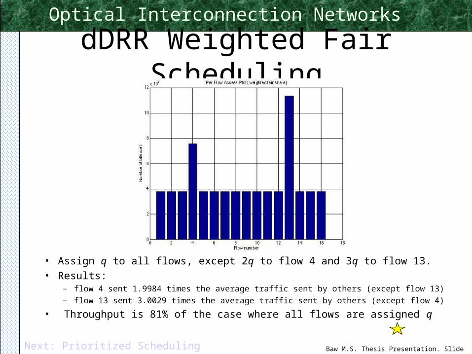
dDRR Weighted Fair Scheduling
• Assign q to all flows, except 2q to flow 4 and 3q to flow 13.
• Results:– flow 4 sent 1.9984 times the average traffic sent by others (except flow 13)
– flow 13 sent 3.0029 times the average traffic sent by others (except flow 4)
• Throughput is 81% of the case where all flows are assigned qNext: Prioritized Scheduling
Page 99
Baw M.S. Thesis Presentation. Slide 99
Optical Interconnection Networks
Prioritized Fair Scheduling in Gemini
qi dci spi nri morei qj dcj spj nrj morej qk dck spk nrk morek
qi dci spi nri morei qj dcj spj nrj morej qk dck spk nrk morek
qi dci spi nri morei qj dcj spj nrj morej qk dck spk nrk morek
qi dci spi nri morei qj dcj spj nrj morej qk dck spk nrk morek
class 1
class 2
class 3
class K
Next: Conclusion
Page 100
Baw M.S. Thesis Presentation. Slide 100
Optical Interconnection Networks
Conclusion
• Summary of Thesis Contributions– Extensible interconnection network simulator framework
– VOQ improves Gemini throughput• O(1) time complexity
• O(N) per switch space complexity
– dDRR scheduler adds fair scheduling capability to Gemini• O(1) time complexity
• O(N) per switch space complexity
• Tunable fairness granularity
Next: Future Work
Page 101
Baw M.S. Thesis Presentation. Slide 101
Optical Interconnection Networks
Conclusion• Future Work
– Better understanding of the throughput vs. fairness granularity tradeoff
• better understanding of many-to-many fair scheduling in general.
– Gemini network interface design• need high speed network interface to take advantage of high
bandwidth optical network
– Gemini is only half optical• need to study the electrical half as well
Next Slide: Many-to-Many Fiar Scheduling
Page 102
Baw M.S. Thesis Presentation. Slide 102
Optical Interconnection Networks
Many-to-ManyWeighted Fair Scheduling
(Future Work)• Fundamental tradeoff:
– Example 1: 4-flow, 4-parallel system, assign weights 1:1:1:2• lose 3/8 throughput
– Example 2: 4-flow, 4-parallel system, assign weights 1:1:1:3• lose 1/2 throughput
– Gemini (N2 flow, N-parallel system)• Nature of “fairness” and throughput tradeoff not yet understood.
Page 103
Baw M.S. Thesis Presentation. Slide 103
Optical Interconnection Networks
Many-to-ManyWeighted Fair Scheduling
(Future Work)• Fundamental tradeoff:
– Example 1: 4-flow, 4-parallel system, assign weights 1:1:1:2• lose 3/8 throughput
– Example 2: 4-flow, 4-parallel system, assign weights 1:1:1:3• lose 1/2 throughput
– Gemini (N2 flow, N-parallel system)• Nature of “fairness” and throughput tradeoff not yet understood.
No reason to do fair scheduling heresince resources are not under contention.
Page 104
Baw M.S. Thesis Presentation. Slide 104
Optical Interconnection Networks
Conclusion
• Future Work– Other optical technologies
• “Smart Pixel Array” and free-space optics
• Extend ICNS framework to include
– Predicate interconnection network study on target applications
• demonstrate that applications indeed benefit from using an optical network
Page 105
Baw M.S. Thesis Presentation. Slide 105
Optical Interconnection Networks
Acknowledgement
• Advisors:– Dr. Mark A. Franklin, Dr. Roger D. Chamberlain
• Committee Members:– Dr. Jonathan S. Turner, Dr. George Varghese
• NSF and DARPA for financial support