OPTICAL MONITORING AND FORECASTING SYSTEMS FOR HARMFUL ALGAL BLOOMS: POSSIBILITY OR PIPE DREAM?

Oscar Schofield, Joe Grzymski Coastal Ocean Observation Laboratory, Institute of Marine and Coastal Sciences, Rutgers University, New Brunswick, New Jersey 08901

W. Paul Bissett Florida Environmental Research Institute, 4807 Bayshore Boulevard, Suite 101, Tampa, Florida 33611

Gary J. Kirkpatrick Mote Marine Laboratory, 1600 Thompson Parkway, Sarasota, Florida 34236

David F. Millie Agricultural Research Service, U.S. Department of Agriculture, New Orleans, Louisiana and Mote Marine Laboratory,

1600 Thompson Parkway, Sarasota, Florida 34236

Mark Moline Department of Biological Sciences, California Polytechnic State University, San Luis Obispo, California 93407

and

Collin S. Roesler Bigelow Laboratory for Ocean Sciences, West Boothbay Harbor, Maine 04575

Monitoring programs for harmful algal blooms Field data will provide inputs to optically based eco­(HABs) are currently reactive and provide little or no system models, which are fused to the observational means for advance warning. Given this, the devel- networks through data-assimilation methods. Poten­opment of algal forecasting systems would be of tial model structure and data-assimilation methods great use because they could guide traditional mon- are reviewed. itoring programs and provide a proactive means for

Key index words: bio-optics; forecasting; harmful al-responding to HABs. Forecasting systems will require gal blooms; remote sensing near real-time observational capabilities and hydro­

dynamic/biological models designed to run in the forecast mode. These observational networks must

An early forecasting system ‘‘The oyster is unsea­detect and forecast over ecologically relevant spatial/ sonable and unwholesome in all months that have temporal scales. One solution is to incorporate a mul­not the letter ‘r’ in their name.’’ Henry Buttes from tiplatform optical approach utilizing remote sensing Dyets Dry Dinner, 1599 (The Handbook of Quotations, and in situ moored technologies. Recent advances in Classical & Medieval).instrumentation and data-assimilative modeling may

Predicting and monitoring harmful algal blooms provide the components necessary for building an (HABs) is central to developing proactive strategies algal forecasting system. This review will outline the to ameliorate their impact on human health and the utility and hurdles of optical approaches in HAB de-economies of coastal communities. As part of these tection and monitoring. In all the approaches, the efforts, numerous coastal monitoring programs have desired HAB information must be isolated and ex-been enacted. Monitoring programs have tradition­tracted from the measured bulk optical signals. Ex-ally detected HABs by visual confirmation (water dis­amples of strengths and weaknesses of the current coloration and fish kills), illness to fish consumers approaches to deconvolve the bulk optical properties (Carder and Steward 1985, Riley et al. 1989, Pierce are illustrated. After the phytoplankton signal has

tion algorithms will be species-specific, reflecting the

been isolated, species-recognition algorithms will be required, and we demonstrate one approach devel-oped for Gymnodinium breve Davis. Pattern-recogni­

1965). Most of the traditional techniques are labor Baden 1990), or mouse bioassays (McFarren et al. shellfish samples (Schulman et al. 1990, Trainor and et al. 1990), chemical analyses for toxin levels in

intensive, which limits the temporal and spatial res-acclimation state of the HAB species of interest. olution of the potential monitoring programs. These sampling limitations bias our understanding of harmful taxa and the environmental conditions promoting bloom initiation, maintenance, and se­

Spatial Scales

Imm lcm 1m 10m 100m lkm 10km 100km

AutonomousVehicles research vessels

I

nescence. Developing approaches to characterize the different stages of phytoplankton-bloom dynam­ics will ultimately require a suite of approaches to provide sufficient sensitivity to detect dilute popu­lations of specific species in mixed phytoplankton communities.

Over the past two decades, oceanographers have de­veloped optical instrumentation that can collect data in a nonintrusive manner [cf. Limnology and Ocean­ography 1989: vol. 34(8) and Journal of Geophysical Research 1995: vol. 100(C7)]. Optical techniques are amenable to a variety of platforms (satellites, aircrafts, mooring, and profiling instrumentation) allowing re­searchers to design multiplatform sampling networks capable of collecting data over ecologically relevant scales (Smith et al. 1987, Fig. 1). Many integrated ob­serving systems currently are under development by the oceanographic community. These approaches show much promise in mapping the distribution of phytoplankton and will be useful in monitoring HABs (Cullen et al. 1997). Furthermore, combining optical approaches with ocean forecast systems (Mooers 1999) would potentially provide water-quality manag­ers a means to prepare for anticipated problems. Al­though promising, optical approaches have been criticized because they provide only bulk composite signals for a water mass, and the signatures for dis­tinct phytoplankton species are difficult to discrim­inate (Garver et al. 1994).

Recent advances in instrumentation, bio-optical models, and coupled observation network/model sys­tems may offer new tools to tackle these issues. Therefore, in this paper we will focus on approaches that we believe show promise and hope to provide consideration of the strengths and weaknesses of the technologies available as of today. Specifically, our discussion will focus on the strengths and weaknesses of in situ optical data in relation to HABs, examine

FIG. 1. The relevant tempo­ral and spatial scales for critical processes regulating phyto­plankton ecology (circles) and the sampling capabilities of the diverse sampling platforms available (squares). Redrawn and modified from Dickey (1993).

optically based ecosystem models which utilize in situ field data, and briefly outline the potential of data-assimilation approaches for the study of HABs. De­veloping a biological ocean forecasting system is a truly interdisciplinary effort, and a comprehensive re­view of all the pertinent aspects is beyond a single manuscript; therefore, we have focused our discus­sion on those approaches with which we are familiar. Given this, we recognize that our discussion may have omitted approaches that might be central to any fu­ture forecasting system. For this discussion, we will omit optical detection of phycobilin-containing HABs, such as cyanobacteria, and will focus primarily on chlorophyll a and chlorophyll c–containing algae. Whenever possible, field data will be used to illustrate both the strengths and weaknesses of these methods. The majority of the data presented was collected in the Gulf of Mexico as part of a multi-institution effort (http://www.fmri.usf.edu/ecohab/) that focused on defining the ecology of the dinoflagellate Gymnodin­ium breve Davis. More detailed description of the data will be provided in forthcoming manuscripts, the data here is used to only illustrate potential strengths and shortcomings. Finally a complete description of the uses of hydrological optics to study phytoplank­ton is well beyond the scope of a single paper. For a more complete treatment of the subject, there are a number of excellent synthetic texts available (Kirk 1994, Mobley 1994, Bukata et al. 1995).

IN SITU OPTICAL MEASUREMENTS

Significant effort over the last decade has focused on developing techniques to measure the spectral dependency of in situ inherent optical properties (IOPs). The advantage of the IOPs is that they de­pend only on the medium and are independent of the ambient light field. This makes them easier to

0.6 0Itt"" before water calibration

0.4 after water calibration....

. .

...........................

0.01

0.3,.--------------,

700

20:00

modeled particulate absorption

15:00local daylight time

measured particu late absorption

500 600wavelength (nm)

""'-"

.......

+- measured total absorption

modeled eDOM absorption

10:00

ol'D~)__-.----:~==~·;;;·...".~~400

20

§.~

£ 0.1-'l

~

-~ 0.2-

-0.2A)

400 500 600 700wavelength (om)

1.2

c .....,..- particulate sJ)Cctra0 " \~ 0.80 \ \•-'l 0.6 ~ \ detriru'•>.~

OA"E eDQM

0.2 "-...'.::C)

0400 450 500 550 600 650 700

wavelength (nm)

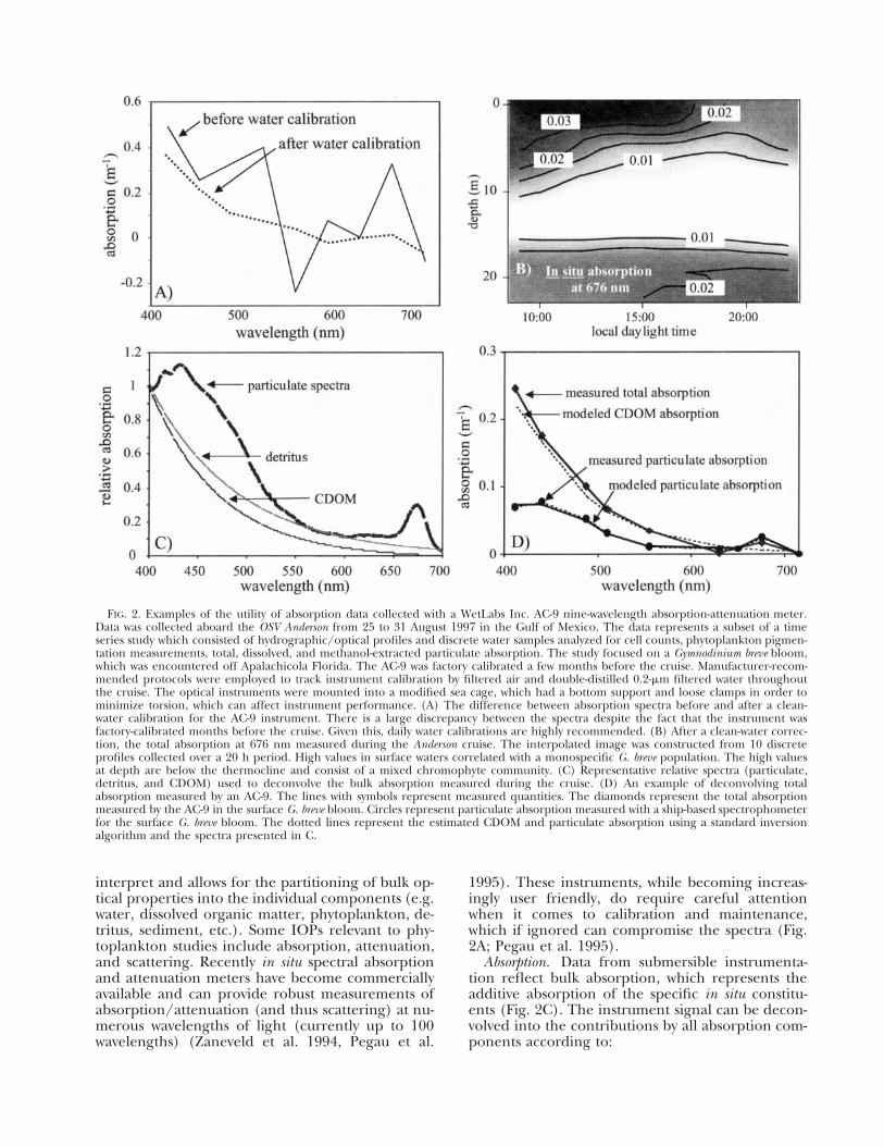
FIG. 2. Examples of the utility of absorption data collected with a WetLabs Inc. AC-9 nine-wavelength absorption-attenuation meter. Data was collected aboard the OSV Anderson from 25 to 31 August 1997 in the Gulf of Mexico. The data represents a subset of a time series study which consisted of hydrographic/optical profiles and discrete water samples analyzed for cell counts, phytoplankton pigmen­tation measurements, total, dissolved, and methanol-extracted particulate absorption. The study focused on a Gymnodinium breve bloom, which was encountered off Apalachicola Florida. The AC-9 was factory calibrated a few months before the cruise. Manufacturer-recom­mended protocols were employed to track instrument calibration by filtered air and double-distilled 0.2-�m filtered water throughout the cruise. The optical instruments were mounted into a modified sea cage, which had a bottom support and loose clamps in order to minimize torsion, which can affect instrument performance. (A) The difference between absorption spectra before and after a clean-water calibration for the AC-9 instrument. There is a large discrepancy between the spectra despite the fact that the instrument was factory-calibrated months before the cruise. Given this, daily water calibrations are highly recommended. (B) After a clean-water correc­tion, the total absorption at 676 nm measured during the Anderson cruise. The interpolated image was constructed from 10 discrete profiles collected over a 20 h period. High values in surface waters correlated with a monospecific G. breve population. The high values at depth are below the thermocline and consist of a mixed chromophyte community. (C) Representative relative spectra (particulate, detritus, and CDOM) used to deconvolve the bulk absorption measured during the cruise. (D) An example of deconvolving total absorption measured by an AC-9. The lines with symbols represent measured quantities. The diamonds represent the total absorption measured by the AC-9 in the surface G. breve bloom. Circles represent particulate absorption measured with a ship-based spectrophometer for the surface G. breve bloom. The dotted lines represent the estimated CDOM and particulate absorption using a standard inversion algorithm and the spectra presented in C.

interpret and allows for the partitioning of bulk op- 1995). These instruments, while becoming increas­tical properties into the individual components (e.g. ingly user friendly, do require careful attention water, dissolved organic matter, phytoplankton, de- when it comes to calibration and maintenance, tritus, sediment, etc.). Some IOPs relevant to phy- which if ignored can compromise the spectra (Fig. toplankton studies include absorption, attenuation, 2A; Pegau et al. 1995). and scattering. Recently in situ spectral absorption Absorption. Data from submersible instrumenta­and attenuation meters have become commercially tion reflect bulk absorption, which represents the available and can provide robust measurements of additive absorption of the specific in situ constitu­absorption/attenuation (and thus scattering) at nu- ents (Fig. 2C). The instrument signal can be decon­merous wavelengths of light (currently up to 100 volved into the contributions by all absorption com­wavelengths) (Zaneveld et al. 1994, Pegau et al. ponents according to:

n

a(�) � � xi ·ai(�) i�1

where ai(�) refers to absorption at wavelength � for component x. Because the instruments are calibrat­ed relative to pure water, the bulk signal can be op­erationally separated into particulate and dissolved material:

atotal � awater � adissolved � aparticulates

and the particulate material can be further parti­tioned into functional groups:

aparticulates � aphytoplankton � asediments � adetritus

Particulate absorption. Given equation 3, deriving the estimates of particulate absorption requires in­version algorithms to extract the particulate signa­ture from other constituents that often dominate the bulk optical properties in coastal waters (Mor­row et al. 1989, Roesler et al. 1989, Bricaud and Stramski 1990, Gallegos et al. 1990, Cleveland and Perry 1994, Roesler and Zaneveld 1994). These in­version techniques are based on modeling the vol­umetric absorption using generalized absorption spectral shapes for one or more of the individual absorbing components or using absorption ratios of different wavelengths that vary in a predictable way according to the components present. The first step in deriving a particulate spectra, involves modeling or measuring the absorption due to Colored Dis­solved Organic Matter (CDOM) so it can be re­moved from the bulk absorption spectra. The CDOM absorption (or gelbstoff) can be described as (Kalle 1966, Bricaud et al. 1981, Green and Blough 1994, CDOM spectra in Fig. 2C),

aCDOM(�) � aCDOM(�440 nm)exp[�S·(� � �440 nm)]

The exponential ‘‘S ’’ parameter (nm-1) depends on the composition of the CDOM present and can vary over 40% with values in marine systems ranging from 0.011 to 0.019 (Carder et al. 1989, Roesler et al. 1989), but many freshwater systems, estuaries, and enclosed oceans exhibit even greater variability in S (Jerlov 1976, Kirk 1977). The exponential co­efficient also depends upon the wavelength range; generally the value increases as the range extends into the ultraviolet wavelengths. Given a value for S and some idealized absorption spectrum for partic­ulates (average spectral shape from independent data sets, see Fig. 2C), the measured bulk absorp­tion spectrum (Fig. 2D) can be deconvolved into volumetric particulate and CDOM absorption using iterative curve fitting procedures. This technique can provide accurate estimates of particulate absorp­tion (Fig. 2D; R2 � 0.88 between measured and pre­dicted absorption for larger unpublished Gulf of Mexico database). The accuracy of these techniques vary significantly with the chosen value of S. This sen­sitivity is likely due to the influence of tripton or detritus which also displays an exponential absorp­

tion coefficient, albeit with a flatter slope (Roesler et al. 1989). Thus, a steeper S can be indicative of the dominance by CDOM, whereas a lower S value indicates potential dominance of particulate organic material. Although these techniques are promising, they will require parameterization of the S value and some generalized absorption data tailored to the specific study site. Given this, collecting spectral li­braries of the absorption characteristics in the field remains of paramount importance.

Another useful approach that circumvents the as­sumption of an idealized wavelength dependency for the total absorption and CDOM is based on mak­ing in situ measurements with and without 0.2-�m filters on the intakes of the instruments (Boss et al. 1998, Roesler 1998, Schofield et al. 1999). The result­ing bulk and dissolved spectra can be used to derive particulate absorption with no a priori assumptions about its wavelength dependency (Fig. 3A). An ex­ample of a particulate spectrum derived using this approach is presented for a phytoplankton bloom encountered in the coastal waters off New Jersey. The particulate spectrum exhibited a blue to red ratio of 2.5 that is representative of phytoplankton (Prezelin and Boczar 1986) (Fig. 3A), and CDOM showed little absorption in the red wavelengths of light with absorption increasing exponentially with decreasing wavelength (Fig. 3A). The high absorp­tion at 715 nm and high absorption at 414 nm re­flects the significant presence of detritus and sedi­ment, which emphasizes that this technique pro­vides a particulate spectrum that can represent many constituents (eq. 3). If refined, these tech­niques offer the potential to generate continuous maps of particulate absorption both as a function of depth and wavelength (Fig. 3B). Furthermore, these approaches are quite amenable for shipboard appli­cations and do not require assumptions about S or some idealized absorption spectra. One potential source of data biasing may be induced by changes in the flow rate of water through the filtered instru­ment compared to the unfiltered one causing ap­parent differences in the depth of features. A sec­ond source of biasing occurs with differential filter clogging which causes sequential restriction in the nominal ‘‘size’’ of the CDOM that passed through the absorption meter. Unless in situ filter replace­ment is used, this approach may not be optimal for moored applications

Phytoplankton spectra. Once a particulate spectrum has been derived, it must be deconvolved into the respective absorption of phytoplankton, detritus, and, if necessary, sediments. A series of different models and approaches have been developed to sep­arate algal and nonalgal absorption from each oth­er. The detrital-absorption spectrum can be approx­imated using an exponential function similar to equation 4; however, the S value is lower than that of CDOM (exponential coefficient for a reference wavelength at 400 nm ranges from 0.006 to 0.014

600650700550 )

450500 tb (nl'l'1Jave\en'ib700

A)1.5 r---.----------

1 --Total (- filter)

~ 1 j.9

e. j~~0.5 j

1Io "--~- _~--__-----==-=::;::::::J

400 450 500 550 600 650

Wavelength (nm)

FIG. 3. (A) A representative set of repetitive measurements with and without a 0.2-�m filter on the AC-9 to provide estimates of the dissolved and total absorption at the depth of the thermocline off the coast of New Jersey on 24 July 1998. Again, manufacturer-recommended protocols for the AC-9 were used. The particulate spectra (resembling phytoplankton absorption) were derived by sub­tracting the dissolved from the total absorption and the resulting spectra. (B) The derived particulate absorption spectra as a function of depth for a station off the coast of New Jersey on 24 July 1998.

nm�1; Roesler et al. 1989). Often, approaches have exploited this and the observed low variance in dis­tinct wavelength ratios in phytoplankton absorption to separate algal and nonalgal spectra (Bricuad and Stramski 1990). Other approaches utilize multiple linear (Morrow et al. 1989) or nonlinear Gaussian-based regression techniques (Hoepffner and Sath­yendranath 1993). The accuracy of these techniques can vary with location (Varela et al. 1998); therefore it is recommended that initial efforts focus on de­veloping criteria for determining which technique is appropriate for a given field site (Varela et al. 1998). Unfortunately for HAB-specific studies, the variance between the measured and derived spectrum can be noisy or so generalized that it compromises the utility of phytoplankton species identification algorithms (see below). Given this, separating the phytoplank­ton absorption from the particulate spectrum will be a central problem for HAB applications.

Species identification. Assuming that a phytoplank­ton absorption spectrum can be derived from a bulk optical measurement, techniques for delineating the presence and quantity of HAB species in a hetero­geneous phytoplankton community are required. Delineation of a particular species can be successful only if the species represents a significant fraction of the overall phytoplankton biomass and/or if it has discriminating features in the cellular optical properties. Differences in the absorption properties between algae can be due to either unique pigments (Jefferey et al. 1997) and/or the light acclimation state associated with the ecological niche occupied by the HAB species.

Laboratory work suggests that partial discrimination of algal species from cellular absorption is possible. For example, Johnsen et al. (1994), using stepwise dis­criminant analyses to classify absorption spectra among 31 bloom-forming phytoplankton (represent­ing the four main groups of phytoplankton with re­spect to accessory chlorophylls; that is, chlorophyll b,

chlorophyll c1, and/or c2, chlorophyll c3, and no ac­cessory chlorophyll), differentiated toxic chlorophyll c3–containing dinoflagellates and prymnesiophytes from taxa not having this pigment. However, problem­atic and toxic taxa could not be further separated from other chlorophyll c3–containing taxa because of the similarities among absorption spectra. Millie et al. (1997) also utilized stepwise discriminant analyses to differentiate mean-normalized absorption spectra for laboratory cultures of G. breve from absorption spectra of a diatom, a prasinophyte, and peridinin-containing dinoflagellates. Therefore, absorption sometimes may provide enough information to distinguish among ab­sorption spectra between phylogenetic groups, and potentially taxa. However, wavelengths delineated by the stepwise techniques were wavelengths associated with the accessory carotenoids. This is problematic as the relative absorption in green, yellow, and orange wavelengths where the carotenoids absorb light is much less when compared to the absorption by chlo­rophyll in the blue and red wavelengths of light. Fur­thermore, the absorption attributable to unique ac­cessory pigments is difficult to discern because of the dampening of the shoulders on absorption spectra from pigment packaging effects (Duysens 1956, Morel and Bricaud 1986). In addition, the spectral depen­dency in the absorption properties of marine chloro­phyll c–containing algae exhibits little variability among taxa (Roesler et al. 1989, Garver et al. 1994, Johnsen et al. 1994).

In order to maximize the minor inflections in spectral absorption, fourth-derivative analysis (But­ler and Hopkins 1970) has been used to resolve the positions of absorption maxima attributable to spe­cific photosynthetic pigments (Bidigare et al. 1989, Smith and Alberte 1994, Millie et al. 1995). Millie et al. (1997) combined derivative analysis with a sim­ilarity index to detect the quantity of G. breve for mixed laboratory phytoplankton cultures (Fig. 4A, B). In brief, fourth-derivative spectra initially were

~ "2.5 2.4 '0 :cI:: c::: ······0% G b u0 Mixed Assemblages of Q) tSB '" .... 20% . reve

~ 2 "0.... ;> 1.8 '0 - 40%~ 2.0 G. breve & Green Algae ..... " 8 ~.@I:: I:: .....'" - 60%

I:':l 0 ......... 0% G. breveI:':l :2 ~ 2 - 80% <.J.......... ;> 1.2 "

u .Q ~ - 100% ~0.. ..... .....1.5 •••• 20% I-< :2 '" ~o fr - 40% Q) U 0.... 0 0% G. breve - 60% Cl 0.6>-'00

..o,D 1.0 - 80% -=~<C - 100% .....I-< 0.0..... ;::sI:':l.....

0.5 00 u... -0.6~ A) B

0.0 -1.2400 500 600 700 400 500 600 700

Wavelength (nm) Wavelength (nm)

1.00C) ...- 0.9...- Ab*A D) ~/

/ SI _ c • "1'>< / ><Q) 0.82 / -IAb\X IAcl Q) 0.8

"'d / "'d ~I:: / I::- / - 0.7 ~ • .,>-. / >-. •''E: 0.64

/ ...../ ..... •/ I-<

I:':l / I:':l 0.6 •- -..... I .....S I S

CI5 0.46 I .....I UJ 0.5I

I~I Hypothetical Mixed Assemblages Natural Populations from GOMx

0.28 0.4 ••0 20 40 60 80 100 0 0.2 0.4 0.6 0.8 1

% G. Breve % G. BreveFIG. 4. (A) Absorption for a hypothetical mixed assemblage of Dunaliella tertiolecta and Gymnodinium breve. The individual spectra

reflect various proportions of the dinoflagellate and green algae ranging from 0% to 100% G. breve (redrawn from Millie et al. 1997). (B) The fourth-derivative spectra for the mixed assemblage spectra presented in A. The individual pigments associated with the specific shoulders in the derivative spectra are delineated (redrawn from Millie et al. 1997). (C) The relationship between the similarity index (eq. 6) versus the relative proportion of G. breve for hypothetical mixed assemblages. (D) Similarity-index values associated with natural mixed phytoplankton population encountered in the Gulf of Mexico (Fig. 2B). This dinoflagellate is the only species of phytoplankton in the eastern Gulf of Mexico observed to contain the pigment gyroxanthin-diester and it appears in constant proportion to cellular chlorophyll a in G. breve. Quantifying gyroxanthin-diester and chlorophyll a allowed to estimate the fraction of the chlorophyll biomass in mixed populations associated with G. breve. Particulate absorption spectra were measured using the quantitative filter technique (QFT) (Kiefer and Soohoo 1982). Sample and reference filters were placed directly in front of the detector windows of a scanning dual-beam spectrophotometer (DMS80, Varian) to minimize scattering loss. Reference spectra for this analysis were collected from a monospecific bloom of G. breve. The data compilation represents samples collected over the course of the year in diverse locations in the Gulf of Mexico. The open circle indicates an estuarine bloom of Cryptoperidinium which has a similar pigment complement but is not found in marine waters associated with G. breve.

computed for mean normalized absorption spectra. The spectral similarity index was determined by computing the angle between the vectors compris­ing the fourth-derivative spectra of a standard G. breve sample from the laboratory and an ‘‘unknown’’ mixed assemblage of phytoplankton as:

A ·Astd unkSI � [ ]�A � � �A �std unk

where Astd and Aunk are the fourth-derivative spectra for G. breve and the unknown samples respectively, ‘·’ is the vector dot-product operator, and �A� is the vector magnitude operator. This approach showed promise in delineating the presence of G. breve for

hypothetical mixed assemblages in the lab (Fig. 4C). More recently this approach has been applied to natural mixed assemblages of G. breve within the Gulf of Mexico. In this field database, G. breve con­tributed between zero to 100% of the measured chlorophyll a. Results for these natural mixed pop­ulations (Fig. 4D) supported the laboratory findings of Millie et al. (1997) that the absorption due to G. breve may be detectable using the derivative/similar­ity-index approach (Kirkpatrick et al. 1999).

Gymnodinium breve contains the unique chemotax­onomic carotenoid gyroxanthin-diester (Millie et al. 1995); however this accessory pigment does not have unique absorption properties and is not re­sponsible for imparting G. breve’s unique absorption

.•

!Ill --iii liD

10:00 15:00 20:00local daylight time

)

5

o

20

•

~ ..•••

50,-----------------,

4 .. •,-,Al/I)----+--------<e---------jo~

o 0.2 0.4 0.6Colored Dissolved Organic MaUer Absorption (at 400 nm, m· l )

20

Coastal Ocean•

rmDliJ ,

,

5 10 15Station

Turbid River & Estuary

•

375e5

oQ. 750

<-0,., 650~..". 550

",. 450"0~. 350

'0"r.",

~

~ 1000 .....

"~ § 500

•"

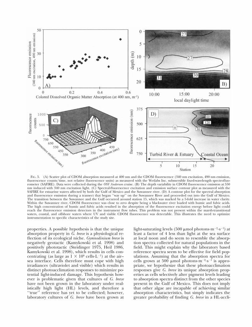
FIG. 5. (A) Scatter plot of CDOM absorption measured at 400 nm and the CDOM fluorescence (340 nm excitation, 490 nm emission, fluorescence counts/time, not relative fluorescence units) as measured with the Wetlabs Inc. submersible fixed-wavelength spectrofluo­rometer (SAFIRE). Data were collected during the OSV Anderson cruise. (B) The depth variability in CDOM fluorescence emission at 550 nm induced with 340 nm excitation light. (C) Spectral-fluorescence excitation and emission surface contour plot as measured with the SAFIRE for estuarine waters affected by both the Gulf of Mexico and the Suwannee river. (D) A contour plot for the spectral absorption and fluorescence emission during a transect that began ‘‘way up’’ on the Suwannee River and proceeded out into the Gulf of Mexico. The transition between the Suwannee and the Gulf occurred around station 15, which was marked by a 5-fold increase in water clarity. Within the Suwannee river, CDOM fluorescence was close to zero despite being a blackwater river loaded with humic and fulvic acids. The high concentration of humic and fulvic acids resulted in the absorption of the fluorescence excitation energy before light could reach the fluorescence emission detectors in the instrument flow tubes. This problem was not present within the marsh-transitional waters, coastal, and offshore waters where UV and visible CDOM fluorescence was detectable. This illustrates the need to optimize instrumentation to specific characteristics of the study site.

properties. A possible hypothesis is that the unique absorption property in G. breve is a physiological re­flection of its ecological niche. Gymnodinium breve is negatively geotactic (Kamykowski et al. 1998) and positively phototactic (Steidinger 1975, Heil 1986, Kamykowski et al. 1998), which results in cells con­centrating (as large as 1 � 108 cells·L�1) at the air– sea interface. Cells therefore must cope with high irradiances (ultraviolet and visible) which results in distinct photoacclimation responses to minimize po­tential light-induced damage. This hypothesis how­ever is problematic given that cultures of G. breve have not been grown in the laboratory under real­istically high light (HL) levels, and therefore a ‘‘true’’ reference has yet to be collected; however, laboratory cultures of G. breve have been grown at

light-saturating levels (500 �mol photons·m�2·s�1) at least a factor of 4 less than light at the sea surface at local noon and do seem to resemble the absorp­tion spectra collected for natural populations in the field. This might explain why the laboratory based reference spectra seem to be effective for field pop­ulations. Assuming that the absorption spectra for cells grown at 500 �mol photons·m�2·s�1 is appro­priate, we hypothesize that these photoacclimation responses give G. breve its unique absorption prop­erties as cells selectively alter pigment levels leading to absorption spectra distinct from the other species present in the Gulf of Mexico. This does not imply that other algae are incapable of achieving similar absorption characteristics, but simply indicates the greater probability of finding G. breve in a HL-accli­

FIG. 6. The ecological and bio-optical interactions in the EcoSim 1.0 model. Squares outlined with bold lines represent optically active processes (i.e. those processes mediated by spec­tral light). Ovals represent optically active constituents (i.e. those constituents that modify the water column light field).

mated state. This feature may be applicable to other HAB species that often exhibit high growth rates and tolerance to bright light (Carlson and Tindall 1985, Johnsen and Sakshaug 1993). This HL envi­ronment also results in enhanced cellular concen­trations of UV absorbing compounds (Vernet et al. 1989). Recognizing this, Kahru and Mitchell (1998) increased the sensitivity-discrimination techniques for HABs by extending their measurements into the ultraviolet-A wavelengths of light. Unfortunately, laboratory cultures of G. breve cannot be maintained at realistic HL levels found in nature, therefore lab­oratory HL adapatation is necessary.

Other vector-based, spectral optical-recognition applications have been developed for signal analyses and may provide alternative pattern-recognition tools for phytoplankton optical signatures. These ap­proaches can be combined with other multivariate methods (e.g. neural networks; Lawrence 1994) to enhance the sensitivity of species identification. Fu­ture research should focus on the sensitivity of these pattern-recognition approaches and whether newly developed hyperspectral instruments will provide the required input data for species-identification al­gorithms. Despite promise, several problems re­main. Field measurements of absorption in situ (for example, the Histar absorption-attenuation meter, Wetlabs, Inc., Philmoth, Oregon, is commercially available) and deck-board using a spectrophotome­ter are often noisy. This noise is magnified through analysis/transformation techniques such as the fourth derivative; therefore, improving the signal to noise for in situ optical sensors is important. Fur­thermore, some of these techniques (like derivative spectra) will require hyperspectral (1–3 nm resolu-

TABLE 1. Ocean color satellites which will be available in the coming years and the respective satellite characteristics. The delayed resolution specifies the data resolution if data is distributed through the individual federal and international agencies. Real-time resolution is the resolution of the satellite through direct broadcast from the satellite.

Operational Satellite (sensor) Country, no. of channels Data rate (mb/sec) Delayed resolution (m) Real-time resolution (m) Revist time (days) (launch date)

NEMO U.S.A, COIS 240 150 30–60 30–60 2.5 1999

EOS AM1 U.S.A, MODIS 2 n/a 250 MODIS 5 n/a 500 MODIS 29 13 n/a 1000 2 1999

EOS PM1 U.S.A, MODIS 2 n/a 250 MODIS 5 n/a 500 MODIS 29 13 n/a 1000 2 2000

EO-1 U.S.A, ALI 10 250 30

HYPERION 256 105 250 30 16 (tiltable) Dec. 1999 HY-1 China,

COCTS 10 4000 1000 2 CZI 4 5.4 4000 250 6 2000

IRS-P4 India, OCM 8 10.4 1800 360 2 1999

ADEOS-2 Japan, GLI 6 1000 250 GLI 30 6 1000 1000 2 2000

�

TABLE 2. Definitions for the EcoSim model variables and parameters.

Definition Symbol Units

Total absorption coefficient Water absorption coefficient Living biomass absorption coefficient Total colored degradational matter absorption coefficient Labile colored dissolved organic carbon absorption coefficient Relict colored dissolved organic carbon absorption coefficient Weight-specific absorption of individual pigments Weight-specific absorption of CDOC1 at 410 nm Weight-specific absorption of CDOC2 at 410 nm Total backscattering coefficient Scattering coefficient of water Scattering coefficient of particulates Backwards proportion of water scattered photons Backwards proportion of particulate scattered photons Total colored degradational matter Labile colored dissolved organic carbon Relict colored dissolved organic carbon Direct downwelling irradiance just beneath the surface Diffuse downwelling irradiance just beneath the surface Downwelling irradiance Total downwelling irradiance Scalar irradiance Total scalar irradiance Functional Group 1—Prochlorococcus (low light) Functional Group 2—Prochlorococcus (high light) Functional Group 3—Synechococcus Functional Group 4—Chromophycota (golden-browns) Downwelling diffuse attenuation coefficient Reduction in absorption resulting from pigment packaging Actual carbon to chlorophyll a ratio Optimal light-limited carbon to chlorophyll a ratio Optimal nutrient-limited carbon to chlorophyll a ratio Intercept of light-limited C:chl a versus light function Intercept of nutrient-limited C:chl a versus light function Slope of light-limited C:chl a a versus light function Slope of nutrient-limited C:chl a versus light function Actual C:chl a ratio C:chl a ratio towards which phytoplankton strive Average cosine of downwelling photons Average cosine of downwelling photons from direct sunlight Average cosine of downwelling photons from diffuse sunlight Average cosine of downwelling photons from total sunlight

at(�, z) aw(�, z) aph(t)(�, z) aCDOM(�, z) aCDOC1

(�, z) aCDOC2

(�, z) a* (�, z)pig a* (410)CDOC1 a* (410)CDOC2 bbt(�, z) bw(�, z) bp(�, z) �bbw �bbp(�, z) CDOM CDOC1 CDOC2 Edir(�, 0�) Edif(l, 0�) Ed(�, z) Ed(z) E0(�, z) E0(z) FG1 FG2 FG3 FG4 Kd(�, z) Package effect

�opt(ll) �opt(nl) �0(ll) �0(nl)slope�(ll)slope�(nl)R Rw ��d(�, z) ��dir(�, 0-) ��dif(�, 0-) ��0(�, 0-)

m�1

m�1

m�1

m�1

m�1

m�1

m2 · mg�1

m2 · g�1

m2 · g�1

m�1

m�1

m�1

Unitless Unitless �M C or �g C L�1

�M C or �g C L�1

�M C or �g C L�1

�mol quanta m�2 · s�1 · nm�1

�mol quanta m�2 · s�1 · nm�1

�mol quanta m�2 · s�1 · nm�1

�mol quanta m�2 · s�1 · nm�1

�mol quanta m�2 · s�1 · nm�1

�mol quanta m�2 · s�1 · nm�1

�M or �g L�1

�M or �g L�1

�M or �g L�1

�M or �g L�1

m�1

Unitless �g C:�g chl a �g C:�g chl a �g C:�g chl a �g C:�g chl a �g C:�g chl a �g C:�g chl a /(�mol quanta · m�2 · s�1) �g C:�g chl a /[�M C (�M N) �1] �g C:�g chl a �g C:�g chl a Unitless Unitless Unitless Unitless

tion) IOP or fluorescence data (see below). Several new spectrometer systems offer the potential to pro­vide hyperspectral data in the near future. While these transformation approaches can be applied to measurements of the IOPs, care should be taken when applying them to apparent optical measure­ments that are sensitive to the geometrical structure of the light field. Utilization of these techniques will also be dependent on further improvements in ex­tracting phytoplankton spectral absorption from the bulk optical signals. Finally, finding a universal glob­al approach for discriminating all HAB species is a pipe-dream. The similarity-index approach that ap­pears appropriate for blooms of G. breve will not be applicable to all species. For example, HAB species like Alexandrium often represent a minor subset of the total phytoplankton community; therefore, the optical signal will often be dominated by the other algal species present. Given this, techniques and ap­proaches will need to be tailored to specific algal species of interest.

Scattering. Light scattering measurements show promise for detecting the concentration and size of particulate material present in seawater (Bricaud and Morel 1986, Stramski and Kiefer 1991, Stramski and Mobley 1997). Most often, the measurements are of the low-angle forward and perpendicular components of the particulate scattering (Trask et al. 1982). These approaches have been most often exploited by flow cytometry with the assumption that small cells had a smaller scattering signal (Perry et al. 1983, Olson et al. 1985, Ackleson and Spinrad 1988). The theory underlying the estimation of par­ticle size from scattering characteristics is based on the Mie theory with anomalous diffraction approxi­mation, whereby the angular distribution of scat­tered light is a function of particle size and the rel­ative refractive index (Van der Hulst 1957, Bricaud et al. 1983, Morel and Bricaud 1986, Stramski and Kiefer 1991). Given this, caution must be used when relating scattering to cell size. For example, the re­fractive index can change by over 80% during a 12

�

�

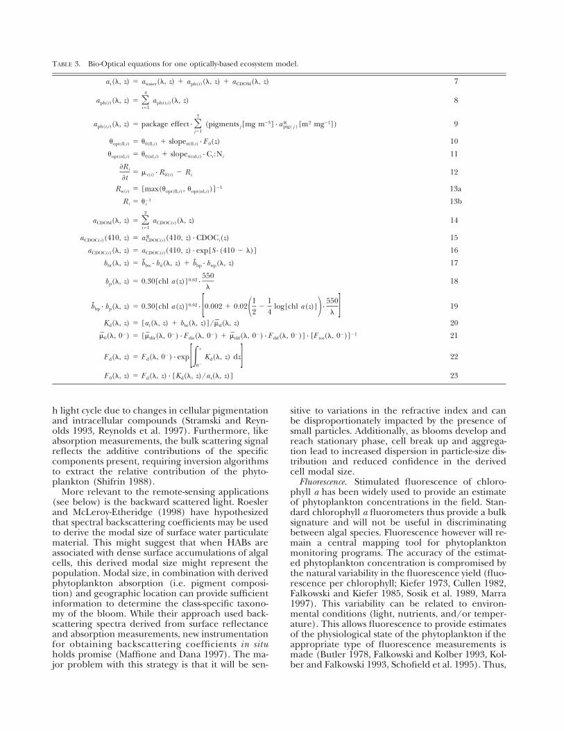
TABLE 3. Bio-Optical equations for one optically-based ecosystem model.

a t(�, z) � awater (�, z) � aph(t)(�, z) � aCDOM (�, z) 7 4

a (�, z) � � a (�, z) 8ph(t) ph(t,i) i�1

7 �3 2 �1a (�, z) � package effect · � (pigments [mg m ] ·a* [m mg ]) 9ph(t,i) j pig( j )

j�1

�opt(ll,i) � � 0(ll,i) � slope�(ll,i) · E0(z) 10

� � � � slope · C :N 11opt(nl,i) 0(nl,i) �(nl,i) i i

�Ri

�t � �r(i) · R w (i) � Ri 12

Rw(i) � [max(�opt(ll,i), �opt(nl,i))]�1 13a �1Ri � �i 13b 2

a (�, z) � � a (�, z) 14CDOM CDOC(i) i�1

a (410, z) � a* (410, z) · CDOC (z) 15 CDOC(i) CDOC(i) i

aCDOC(i)(�, z) � aCDOC(i)(410, z) · exp[S ·(410 � �)] 16

bbt(�, z) � b bw · b w (�, z) � b bp · bwp(�, z) 17

550 bp(�, z) � 0.30[chl a(z)]0.62 · 18

1 1 550 b bp(�, z) � 0.30[chl a(z)]0.62 · 0.002 � 0.02 � log[chl a(z)] · 19˜ bp · [ � � ]2 4 �

Kd(�, z) � [a t(�, z) � bbt (�, z)]/� d(�, z) 20 � � � � � � �1� (�, 0 ) � [� (�, 0 ) · E (�, 0 ) � � (�, 0 ) · E (�, 0 )] · [E (�, 0 )] 210 dir dir dif dif tot

z

E (�, z) � E (�, 0 ) · exp K (�, z) dz 22d d d[� ]0�

E (�, z) � E (�, z) · [K (�, z)/a (�, z)] 230 d d t

h light cycle due to changes in cellular pigmentation and intracellular compounds (Stramski and Reyn­olds 1993, Reynolds et al. 1997). Furthermore, like absorption measurements, the bulk scattering signal reflects the additive contributions of the specific components present, requiring inversion algorithms to extract the relative contribution of the phyto­plankton (Shifrin 1988).

More relevant to the remote-sensing applications (see below) is the backward scattered light. Roesler and McLeroy-Etheridge (1998) have hypothesized that spectral backscattering coefficients may be used to derive the modal size of surface water particulate material. This might suggest that when HABs are associated with dense surface accumulations of algal cells, this derived modal size might represent the population. Modal size, in combination with derived phytoplankton absorption (i.e. pigment composi­tion) and geographic location can provide sufficient information to determine the class-specific taxono­my of the bloom. While their approach used back­scattering spectra derived from surface reflectance and absorption measurements, new instrumentation for obtaining backscattering coefficients in situ holds promise (Maffione and Dana 1997). The ma­jor problem with this strategy is that it will be sen­

sitive to variations in the refractive index and can be disproportionately impacted by the presence of small particles. Additionally, as blooms develop and reach stationary phase, cell break up and aggrega­tion lead to increased dispersion in particle-size dis­tribution and reduced confidence in the derived cell modal size.

Fluorescence. Stimulated fluorescence of chloro­phyll a has been widely used to provide an estimate of phytoplankton concentrations in the field. Stan­dard chlorophyll a fluorometers thus provide a bulk signature and will not be useful in discriminating between algal species. Fluorescence however will re­main a central mapping tool for phytoplankton monitoring programs. The accuracy of the estimat­ed phytoplankton concentration is compromised by the natural variability in the fluorescence yield (fluo­rescence per chlorophyll; Kiefer 1973, Cullen 1982, Falkowski and Kiefer 1985, Sosik et al. 1989, Marra 1997). This variability can be related to environ­mental conditions (light, nutrients, and/or temper­ature). This allows fluorescence to provide estimates of the physiological state of the phytoplankton if the appropriate type of fluorescence measurements is made (Butler 1978, Falkowski and Kolber 1993, Kol­ber and Falkowski 1993, Schofield et al. 1995). Thus,

although not HAB-specific, fluorescence-based pho­tosystem II quantum yield measurements will be key for describing the potential health of the phyto­plankton population.

As described above, the spectral signature of phy­toplankton can potentially be used to detect the presence of HAB species. A technique that is phy­toplankton-specific, highly sensitive in dilute suspen­sions and can provide hyperspectral data on phyto­plankton pigmentation is chlorophyll a fluorescence excitation spectra (Yentsch and Yentsch 1979). The major advantage of these measurements is that the spectrum provides only the signature for the pho­tosynthetic pigments and avoids the confounding signal of nonphotosynthetic pigments (Yentsch and Phinney 1985, Demmig et al. 1987, Maske and Haardt 1987, Schubert et al. 1994) that are present within both nonHAB and HAB species. These stim­ulated fluorescence spectra thus have sharper pig­ment shoulders than corresponding absorption measurements (Schofield et al. 1990, Grzymski et al. 1997, Johnsen et al. 1997), which would increase the power of any pattern-recognition algorithm. Sub­mersible fixed-wavelength spectrofluorometers are available (Spectral Absorption Fluorescence Excita­tion Emission Meter, SAFIRE, Wetalbs Inc.), but to date do not have the spectral resolution required for pattern-recognition algorithms.

The significant presence of CDOM in coastal and inland waters often dominates bulk absorption. This can compromise the accuracy of empirical inversion approaches as described above. A possible means to circumvent this problem is to develop independent means to estimate the in situ concentration of CDOM. Recently, techniques have been developed to characterize CDOM using UV and/or visible light–induced CDOM fluorescence (Hoge and Swift 1981, Coble et al. 1990, Chen and Bada 1992, Green and Blough 1994, Vodacek et al. 1995, Ferrari et al. 1996, Nieke et al. 1997). Commercially available submersible instrumentation can measure UV/visi­ble light–induced fluorescence, thereby providing information on the concentration of CDOM (Fig. 5A) or the absorption of CDOM when the variance in the quantum yield is negligible (Ferrari and Tas­san 1991). Further data is required to determine to what degree these observed relationships are linear over an environmentally relevant range of concen­trations and are robust in both time and space. An example of CDOM fluorescence within 1997 G. breve bloom is presented in Figure 5B. There are, how­ever, several caveats for using fluorescence to de­scribe CDOM. First, calibration and standardization between instrument systems are not trivial, requiring careful consideration of the quantum correction fac­tors to be applied to the instrument signals (Coble et al. 1990). Discrimination of the form of CDOM from fluorescence will only be to a general level (see Fig. 5C that presents the CDOM for estuarine wa­ters). For example, marine CDOM can be differen­

tiated from terrestrial CDOM by its overall low fluo­rescence intensity and the few prominent shoulders in the blue wavelengths of light (Coble et al. 1990, Coble 1996). Finally, the choice of the appropriate excitation–emission wavelengths for CDOM fluo­rometers will vary depending on the field site, given that the high CDOM absorption in UV and visible wavelengths will significantly affect instrument per­formance (Fig. 5D).

REMOTE SENSING

Above water ocean color is determined primarily from the reflectance, defined as the ratio of the up­ward flux of light to downward flux of light incident on the ocean surface. Atmospheric effects aside, re­flectance is a function of both the scattering and absorption properties within the water column. The relationship between reflectance and the IOPs can reasonably be described as the ratio of backscatter to absorption, such as

bb(�)R � G

a(�) � bb(�) where G is a constant dependent on the angular distribution of the light field and the volume scat­tering coefficient (Gordon et al. 1975, Morel and Prieur 1977, Zaneveld 1982, 1995).

Several satellite and aircraft remote-sensing systems currently are in use, each having distinct spectral and spatial resolution (IOCCG 1999). The derived prod­ucts from these systems include chlorophyll a bio­mass, CDOM, sediment, IOPs, primary productivity, and potentially community classification (phycobilin and nonphycobilin-containing algae, Subramaniam et al. 1999a, b). These systems collect data over eco­logically relevant spatial scales, and therefore provide a mechanism to scan for algal productivity ‘‘hot­spots.’’ Given this, they will be key to the mapping of phytoplankton dynamics and provide inputs to coupled biological/hydrodynamic models. Further­more, semianalytical approaches to invert the reflec­tance spectra have been developed and show great promise for refining the interpretation of remote-sensing data (Fischer and Doerffer 1987, Gordon et al. 1988, Doerffer and Fischer 1994, Lee et al. 1994, Roesler and Perry 1995, Garver and Siegel 1997).

The disadvantages of ocean color satellites in­clude the confounding impact of clouds, the limit of detection to near-surface features, the lack of HAB-specific algorithms, the often degraded spatial resolution of the sensor, and the stringent embar­goes of real-time data access for most users. For air­craft sensors, considerations include cost, impact of partial cloud cover, as well as corrections for sensor geometry and atmospheric signals. Real-time full-resolution data from these satellites is accessible via direct-broadcast satellite dishes, which will enable scientists to access the growing international con­stellation of satellites (Table 1). The real-time data from the full constellation of satellites will be critical

to minimize site revisit intervals and potentially pro­vide researchers coverage at different times on the same day for tracking phytoplankton plumes. Development of regional networks of these direct access satellite dish platforms will be critical to the scientific community, much analogous to the im­portance of the proliferation of High Resolution Picture Transmission (HRPT) satellite data-acquisi­tion systems which revolutionized the utility and availability of AVHRR satellite data. Development of these systems will be strongly dependent on in-water validation studies.

ECOSYSTEM MODELS

With the ability to measure in-water optical prop­erties and the promise of algorithms to separate them into individual optical constituents, comes the inevitable question—how will optical data be used to describe HABs? Optically based ecosystem models will be a key tool in providing a means to optimally interpolate to regions where in situ data is sparse (in both space and time), coordinating field sampling efforts, and providing a central component to any forecasting network.

The work by Riley (1946, 1947) on Geogres Bank is often acknowledged as the root for many modern coastal-ecosystem models. While the earliest models varied with time, the environmental complexity was necessarily simplified. The environmental complex­ity of the models has increased with the increase in computing power, and by the 1970s, explicit descrip­tions of circulation patterns were included to de­scribe the physical transport of phytoplankon pop­ulations (Walsh 1975, Wroblewski 1977). Ecosystem models in recent years have with varying degress of success simulated seasonal changes in both chloro­phyll a and/or nutrient fields (Walsh et al. 1989, 1991, Bissett et al. 1994, McClain et al. 1999). Most of the models are based on simplified food webs (Walsh et al. 1999) and thus do not explicitly con­sider the natural phytoplankton diversity despite the fact that community diversity significantly affects foodweb dynamics and biogeochemistry. Given this, current ecosystem models are still a long way from the more specialized need of predicting HABs.

For the purposes of this paper, we focus our dis­cussion on a model being developed for mixed-phy­toplankton communities with the caveats that: (1) any of the available models will require substantial modification for HAB detection; and (2) the de­scribed model represents one of many possible mod­els currently under development by the oceano­graphic community. We have chosen this model as it is designed to utilize the optical signals as inputs for biological parameters, and thus, it could be col­lected using the optical systems described above. The Ecological Simulation (EcoSim) 1.0 model (Fig. 6) has simulated the seasonal succession of phyto­plankton communities and changes in the optical properties in the Sargasso Sea (Bissett et al. 1999a,

b). This model describes the temporal changes in the in situ optical constituents and the effects on water clarity and resulting feedbacks on the ecosys­tem (Tables 2 and 3).

The EcoSim model utilizes the spectral distribu­tion of light energy, along with temperature and nu­trients, to drive the growth of phytoplankton func­tional groups (FG) representing broad classes of the phytoplankton species. For past simulations of the Sargasso Sea, the functional groups consisted of FG1—Prochlorococcus (high chlorophyll b), FG2— Prochlorococcus (low chlorophyll b), FG3—Synechococ­cus, and FG4—Chromophyta (chlorophyll c contain­ing). The intracellular chlorophyll a concentrations of each functional group vary as a function of the light history and nutrient status of the group. Each functional group has its own unique set of accessory pigments, which vary as a function of the carbon to chlorophyll a ratio. Absorption by phytoplankton (eq. 8) is the sum of absorption from each phyto­plankton species modified by the package effect (Morel and Bricaud 1986, eq. 9). Each phytoplank­ton species can chromatically adapt to changes in total photon flux (eq. 10) and intracellular nutrient status (eq. 11) through changes in the cellular car­bon to chlorophyll a ratio. Changes in carbon to chlorophyll a ratios, in turn, lead to changes in ac­cessory pigment concentrations (equations not shown). The time rate of change of the carbon to chlorophyll a ratio is a function of the growth rate of the individual phytoplankton groups (eqs. 12 and 13). Other optically important parameters (eq. 7) are also parameterized with the model (eqs. 14–16).

Light intensity just below the sea surface–atmo­sphere interface, Ed(�, 0�), can be derived using atmospheric radiative transfer models (Gregg and Carder 1990) influenced by the variable presence of clouds. The attenuation of light energy with increas­ing water depth is a function of the distribution of light energy, as well as the spectral absorption and scattering of the water (Fig. 6). The absorption and scattering properties of the ecosystem respond to changes in the downwelling solar energy through cellular growth, loss of biomass, changes in pigmen­tation, and photolysis of CDOM. Similar to absorp­tion, scattering (eq. 17) is assumed to be a linear combination of the individual optical constituents. The equations for particulate scattering and back­scattering (eqs. 17–19) are related to total chloro­phyll a concentration (Morel 1988). The diffuse at­tenuation coefficient (Kd) is linked to the IOPs via an estimation of the geometric structure of the downwelling light field (eq. 20, Fig. 7) (Sathyen­dranath and Platt 1988). This value at the sea sur­face is given by equation 21 (Morel 1988). It is mod­ified with depth as a function of the total scattering to beam attenuation ratio. Thus, with an estimation of Kd, downwelling irradiance can be attenuated (eq. 22) and total scalar irradiance approximated (eq. 23). Model simulations for the optical signa­

Propagating Light Through a Water Column

r1

For eachdepth interval ,. h .__ 19 t attenuatIOn

e(A.,) = a(A,I) + brA,')

absorptionalA,') = aw",,,(A) + aph,,,(A)

+ aCDOM(A) + a=l(A)scatteringb(A.,t) = bwa1c/A) + bphyto(A)

+ bcDDM(A) + b",(A)

backscatteringbb(A.,t) ;:; bb,wateP',) + bb,phYIO(A)

+ bb,cDOM(A) + bb."d(A)

geometric structure of light~d(A) = fxn[b(A,I).e (A ,I), ~(A)]

diffuse light attenuationKd(A) = [a(A,I) + bb(A ,t))/~d(A)]

water leaving radiance toa satellite

L,(A) = fxn[a(A,I),b(A ,I), bb(A .1),

E,(A,I), ~,(A), ~d(A), ~,(A)]

FIG. 7. Schematic view of Ecosim 1.0 bio-optical equations. Each layer in the filled column represents a layer in the EcoSim. The optical equations are solved for each of these layers as light propagates through the model domain.

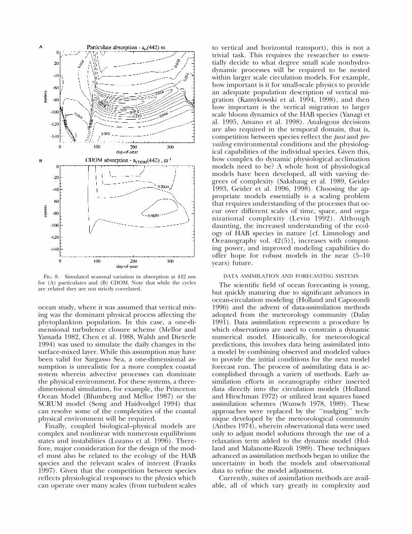
tures of particulates, CDOM, and diffuse attenuation are presented in Figures 8 and 9. Model results agree well with measured in situ data (Fig. 9; Bissett et al. 1999a, b).

Although many of the approximations used in the model are simplistic, they are numerically efficient. This is important at this stage of model develop­ment. In the model, the equations for light propa­gation are limited to the downward direction. More accurate Radiative Transfer Models (RTM) that fully describe the geometric structure of the light field (Mobley 1994) exist; however, resolving the angular distribution of photons in EcoSim 1.0 would have increased the length of each simulation run from hours to tens of years. Although computer-process­

ing speed has increased drastically in recent years, prediction of HABs will require three-dimensional ecological/optical/physical simulations, whose com­putational requirements would currently preclude the use of a complete RTM. Additionally, much more work is required in the field to rigorously test the predictions of the optical-simulation models.

Phytoplankton assemblages respond to an ever-changing physical environment. The rise of a HAB species to bloom proportions is directly related to the past history and current status of the circulation patterns. Thus, the importance of accurately simu­lating the physical environment to future predic­tions of HAB outbreaks cannot be overemphasized. The EcoSim model was developed for an open

A o~~~~._~Particulate absorption - <1",(442) m'

-20

300

300

0.0030

200day-of-year

100

100

200day-of-year

eDOM absorption - aCDOM(442), m-I

0

B0

-20

-40

-60

-80

-100

-120

-140

0

FIG. 8. Simulated seasonal variation in absorption at 442 nm for (A) particulates and (B) CDOM. Note that while the cycles are related they are not strictly correlated.

ocean study, where it was assumed that vertical mix­ing was the dominant physical process affecting the phytoplankton population. In this case, a one-di­mensional turbulence closure scheme (Mellor and Yamada 1982, Chen et al. 1988, Walsh and Dieterle 1994) was used to simulate the daily changes in the surface-mixed layer. While this assumption may have been valid for Sargasso Sea, a one-dimensional as­sumption is unrealistic for a more complex coastal system wherein advective processes can dominate the physical environment. For these systems, a three-dimensional simulation, for example, the Princeton Ocean Model (Blumberg and Mellor 1987) or the SCRUM model (Song and Haidvodgel 1994) that can resolve some of the complexities of the coastal physical environment will be required.

Finally, coupled biological–physical models are complex and nonlinear with numerous equilibrium states and instabilities (Lozano et al. 1996). There­fore, major consideration for the design of the mod­el must also be related to the ecology of the HAB species and the relevant scales of interest (Franks 1997). Given that the competition between species reflects physiological responses to the physics which can operate over many scales (from turbulent scales

to vertical and horizontal transport), this is not a trivial task. This requires the researcher to essen­tially decide to what degree small scale nonhydro­dynamic processes will be required to be nested within larger scale circulation models. For example, how important is it for small-scale physics to provide an adequate population description of vertical mi­gration (Kamykowski et al. 1994, 1998), and then how important is the vertical migration to larger scale bloom dynamics of the HAB species (Yanagi et al. 1995, Amano et al. 1998). Analogous decisions are also required in the temporal domain, that is, competition between species reflect the past and pre­vailing environmental conditions and the physiolog­ical capabilities of the individual species. Given this, how complex do dynamic physiological acclimation models need to be? A whole host of physiological models have been developed, all with varying de­grees of complexity (Sakshaug et al. 1989, Geider 1993, Geider et al. 1996, 1998). Choosing the ap­propriate models essentially is a scaling problem that requires understanding of the processes that oc­cur over different scales of time, space, and orga­nizational complexity (Levin 1992). Although daunting, the increased understanding of the ecol­ogy of HAB species in nature [cf. Limnology and Oceanography vol. 42(5)], increases with comput­ing power, and improved modeling capabilities do offer hope for robust models in the near (5–10 years) future.

DATA ASSIMILATION AND FORECASTING SYSTEMS

The scientific field of ocean forecasting is young, but quickly maturing due to significant advances in ocean-circulation modeling (Holland and Capotondi 1996) and the advent of data-assimilation methods adopted from the meteorology community (Dalay 1991). Data assimilation represents a procedure by which observations are used to constrain a dynamic numerical model. Historically, for meteorological predictions, this involves data being assimilated into a model by combining observed and modeled values to provide the initial conditions for the next model forecast run. The process of assimilating data is ac­complished through a variety of methods. Early as­similation efforts in oceanography either inserted data directly into the circulation models (Holland and Hirschman 1972) or utilized least squares based assimilation schemes (Wunsch 1978, 1989). These approaches were replaced by the ‘‘nudging’’ tech­nique developed by the meteorological community (Anthes 1974), wherein observational data were used only to adjust model solutions through the use of a relaxation term added to the dynamic model (Hol­land and Malanotte-Rizzoli 1989). These techniques advanced as assimilation methods began to utilize the uncertainty in both the models and observational data to refine the model adjustment.

Currently, suites of assimilation methods are avail­able, all of which vary greatly in complexity and

-20

-40

-60~~

E -80

-100

-120

-140

5:1 5:182 5:365 6:182 6:365

Measured Ki488) molor------,.---,----,----,..::-----,.---,----,--------,

-20

-40

-60

~Il) -80E

-IOO~-~-

-120

-140

93:1 93:182 93:365year:day-of-year

94:182 94:365

computational cost making them appropriate for different applications. The Optimal Interpolation (OI) method is a technique where model adjust­ment by observational data depends on the errors in the data, the dynamical constraints of the model, and the error estimate in the model solution (Breth­erton et al. 1976, Dombrowsky and DeMey 1989, Robinson et al. 1989, Mellor and Ezer 1991). This approach has relatively low computational require­ments making it appropriate for high-resolution forecast applications. More advanced schemes, such as the ‘‘Kalman filter/smoother’’ assimilation meth­od (Kalman 1960), are computationally expensive,

FIG. 9. (A) Simulated Kd(487) and (B) measured Kd(488). The measured Kd data was provided by Dr. D. Siegel, University of Califor­nia at Santa Barbara. The bold black line is the mixed layer depth.

which currently limits their use for complex models (Malanotte-Rizzoli and Tzipermann 1996), such as biological/hydrodynamic models that would be re­quired for HAB forecasting applications. Another advanced assimilation scheme is the adjoint method, which is not appropriate for forecasting applications but is a powerful means to perform hindcast dynam­ical analyses. Such an approach will be useful for understanding the environmental conditions asso­ciated with algal bloom initiation from time-series data. Currently, several coupled physical–biological models have been constructed with data-assimilative methods (Ishizaka 1990, Fasham and Evans 1995,

Observation Network(Satellites, Sbips, Moorings, Meteorology)

Adaptive SamplingFeedback

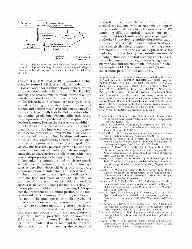
FIG. 10. Schematic for an ocean nowcast/forecast system al­lowing for adaptive sampling of events poorly sampled using tra­ditional shipboard protocols. Schematic adapted from Glenn et al. 1998.

Lawson et al. 1995, Matear 1995) providing a blue­print for future HAB data-assimilative models.

Coastal ocean forecasting networks generally work in a recursive mode (Glenn et al. 1998, Fig. 10). Initially, the data-assimilative model provides a now-cast that is moved forward in time by the circulation model driven by surface-boundary forcing. Surface-boundary forcing is available through a variety of federal and defense weather prediction systems. The forecast cycle generally lasts for 2–4 days after which the weather predictions become sufficiently coarse to compromise any predicted hydrographic or ad­vection features. During the forecast cycle, addition­al field data are assimilated to constrain the model dynamics to provide improved nowcasts for the next set of ocean forecasts. To improve the quality of the nowcasts, adaptive sampling by ships and autono­mous vehicles is initiated to collect subsurface data in specific regions within the forecast grid. Con­versely, the forecasts/nowcasts provide an unprece­dented opportunity for biologists to devise sampling strategies to characterize episodic events, which can play a disproportionately large role in structuring phytoplankton communities and which are poorly sampled using traditional protocols. Therefore, sys­tems as described above will be critical in studying bloom initiation, maintenance, and senescence.

The utility of any forecasting system will vary with both the type and phase of the HAB bloom. For example, optical techniques are likely to have little success in detecting blooms during the earliest ini­tiation phases of a bloom or in detecting HAB spe­cies that represent only a minor portion of the total phytoplankton community. These approaches will also not provide much success in predicting whether a particular bloom is toxic; however it will provide a means to structure monitoring efforts which can then utilize more powerful diagnostic tools. Given this, these approaches will provide researchers with a powerful suite of proactive tools for monitoring HAB populations in nature. For these tools to real­ize their full potential we recommend that research should focus on: (1) increasing the accuracy of

methods to deconvolve the bulk IOPs into the in­dividual constituents, with an emphasis on improv­ing methods to derive phytoplankton spectra; (2) combining different optical measurements to in­crease the utility of multivariate pattern-recognition methods; (3) developing multiplatform observation networks to collect data in horizontal/vertical space over ecologically relevant scales; (4) refining ecosys­tem models to utilize the available optical data; (5) exploring and developing data-assimilation models in conjunction with physical oceanographers to cre­ate early generation biological-forecasting systems; (6) verifying and utilizing model forecasts for adap­tive sampling of HAB phenomena; and (7) surviving the arduous period of trial and error.

Support was provided by numerous agencies including the Office of Naval Research’s COMOP, HyCODE and CMO programs (N00014-97-0767, N0014-99-0196, N00014-98-10251), a National Ocean Partnership Award (N00014-97-1-1019), a USDA-NRI award (96-351010-3122), an EPA grant (R825243), a NASA grant (NAG5-7872), Florida DEP, and the William G. Selby and Marie Selby Foundation. Excellent and constructive reviews by two anonymous reviewers and John Cullen greatly improved this man­uscript. Special thanks and a cold beer is owed to Scott Glenn. We are also very grateful to Trisha Bergmann, Kenneth Carder, Mike Crowley, Tom Fraser, Jennifer Patch, Robert Steward, and Bryan Vinyard. ECOHAB contribution number 6.

Ackelson, S. G. & Spinrad, R. W. 1988. Size and refractive index of individual marine particulates: a flow cytometric approach. Appl. Opt. 27:1270–77.

Amano, K., Watanabe, M., Kohata, K. & Harada, S. 1998. Con­ditions necessary for Chattonella antiqua red tide outbreaks. Limnol. Oceanogr. 43:117–28.

Anthes, R. A. 1974. Data assimilation and initialization of hurri­cane prediction models. J. Atmos. Sci. 31:701–19.

Bidigare, R. R., Morrow, J. H. & Kiefer, D. A. 1989. Derivative analysis of spectral absorption by photosynthetic pigments in the western Sargasso Sea. J. Mar. Res. 47:323–41.

Bissett, W. P., Carder, K. L., Walsh, J. J. & Dieterle, D. A. 1999a. Carbon cycling in the upper waters of the Sargasso Sea: II. Numerical simulation of apparent and inherent optical prop­erties. Deep-Sea Res. 46:271–17.

Bissett, W. P., Meyers, M. B., Walsh, J. J. & Muller-Karger, F. E. 1994. The effects of temporal variability of mixed layer depth on primary productivity around Bermuda. J. Geophys. Res. 99: 7539–53.

Bissett, W. P., Walsh J. J., Dieterle, D. A. & Carder, K. L. 1999b. Carbon cycling in the upper waters of the Sargasso Sea: I. Numerical simulation of differential carbon and nitrogen fluxes. Deep-Sea Res. 46:205–69.

Blumberg, A. F. & Mellor, G. L. 1987. A description of a three dimensional coastal ocean circulation model. In Heaps, N. [Ed.] Three-dimensional Coastal Ocean Models, AGU, Washing­ton DC, pp. 208–33.

Boss, E., Pegau, S., Zaneveld, J. R. V., Barnard, A. H. B. 1998. Spatial and temporal variability of absorption by dissolved material at a continental shelf. SPIE Ocean Optics XIV 2:42– 48.

Bretherton, F. P., Davis, R. E. & Fandry, C. B. 1976. A technique for objective analysis and design of oceanographic experi­ments applied to MODE-73. Deep-Sea Res. 23:559–82.

Bricaud, A. & Morel, A. 1986. Light attenuation and scttering by phytoplanktonic cells: A theorectical modeling. Appl. Opt. 25: 571–80.

Bricaud, A., Morel, A. & Prieur, L. 1981. Absorption by dissolved organic matter of the sea (yellow substance) in the UV and visible domains. Limnol. Oceanogr. 26:45–53.

1983. Optical efficiency factors of some phytoplankters. Limnol. Oceanogr. 28:816–73.

Bricaud, A. & Stramski, D. 1990. Spectral absorption coefficients of living phytoplankton and nonalgal biogenous matter: a comparison between the Peru upwelling area and the Sar­gasso Sea. Limnol. Oceanogr. 35:562–82.

Bukata, R. P., Jerome, J. H., Kondratyev, K. Y. & Pozdnyakov, D. V. 1995. Optical Properties and Remote Sensing of Inland and Coastal Waters. CRC Press, Boca Raton, 362 pp.

Butler, W. L. 1978. Energy distribution in the photochemical apparatus of photosynthesis. Annu. Rev. Plant Physiol. 29:345– 78.

Butler, W. L. & Hopkins, D. W. 1970. An analysis of fourth de­rivative spectra. Photochem. Photobiol. 12:451–56.

Carder, K. L. & Steward, R. G. 1985. A remote-sensing reflec­tance model of a red-tide dinoflagellate off west Florida. Lim­nol. Oceanogr. 30:286–98.

Carder, K. L., Steward, R. G., Harvey, G. R. & Ortner, P. B. 1989. Marine humic and fulvic acids: Their effects on remote sens­ing of chlorophyll a. Limnol. Oceanogr. 34:68–81.

Carlson, R. D. & Tindall, D. R. 1985. Distribution and periodicity of toxic dinoflagellates in the Virgin Islands. In Anderson, D. M. [Ed.] Toxic Dinoflagellates. Elsevier, New York, pp. 171–6.

Chen, R. F. & Bada, J. L. 1992. The fluorescence of dissolved organic matter in seawater. Mar. Chem. 37:191–221.

Chen, D., Horrigan, S. G. & Wang, D. P. 1988. The late summer vertical nutrient mixing in Long Island Sound. J. Mar. Res. 46:753–70.

Cleveland, J. S. & Perry, M. J. 1994. A model for partitioning particulate absorption into phytoplankton and detrital com­ponents. Deep-Sea Res. 41:197–21.

Coble, P. G. 1996. Characterization of marine and terrestrial DOM in seawater using excitation-emission matrix spectros­copy. Mar. Chem. 51:325–46.

Coble, P. C., Green, S., Blough, N. V. & Gagosian, R. B. 1990. Characterization of dissolved organic matter in the Black Sea by fluorescence spectroscopy. Nature 348:432–35.

Cullen, J. J. 1982. The deep chlorophyll maximum: comparing profiles of chlorophyll a. Can. J. Fish. Aquat. Sci. 39:791–803.

Cullen, J. J., Ciotti, A. M. & Lewis, M. R. 1997. Optical detection and assessment of algal blooms. Limnol. Oceanogr. 42:1223– 39.

Dalay, R. 1991. Atmospheric Data Analysis. Cambridge University Press, Cambridge, 497 pp.

Demmig, B., Winter, K., Kruger, A., Czygan, F. C. 1987. Photo-inhibition and zeaxanthin formation in intact leaves; a pos­sible role of the xanthophyll cycle in the dissipation of excess light energy. Plant Physiol. 84:214–24.

Dickey, T. 1993. Sensors and systems for sampling/measuring ocean processes extending over nine orders of magnitude. Sea Tech. 34:47–55.

Doerffer, R. & Fischer, J. 1994. Concentrations of chlorophyll, suspended matter, and gelbstoff in case II waters derived from satellite coastal zone color scanner data with inverse modeling methods. J. Geophy. Res. 99:7457–66.

Dombrowsky, E. & DeMey, P. 1989. Continuous assimilation in an open domain of the Northeast Atlantic, part I: method­ology and application to AthenA-88. J. Geophys. Res. 97:9719– 31.

Duysens, I. N. M. 1956. The flattening of the absorption spec­trum of suspensions, as compared to that of solutions. Bio­chim. Biophys. Acta. 19:1–12.

Falkowski, P. G. & Kiefer, D. A. 1985. Chlorophyll a fluorescence and phytoplankton: Relationship to photosynthesis and bio­mass. J. Plankton Res. 7:715–31.

Falkowski, P. G. & Kolber, Z. 1993. Estimation of phytoplankton photosynthesis by active fluorescence. ICES Mar. Sci. Symp. 197:92–103.

Fasham, M. J. R. & Evans, G. T. 1995. The use of optimazation techniques to model marine ecosystems dynamics at the JGOFS station at 47� N 20� W. Phil. Trans. Roy. Soc. 348:203– 09.

Ferrari, G. M., Dowell, M. D., Grossi, S. & Targa, C. 1996. Rela­

tionship between the optical parameters of chromophoric dissolved organic matter and total concentration of dissolved organic carbon in the southern Baltic Sea region. Mar. Chem. 55:299–16.

Ferrari, G. M. & Tassan, S. 1992. Evaluation of the influence of yellow substance absorption on the remote sensing of water quality in the Gulf of Naples. Inter. J. Rem. Sen. 13:2177–86.

Fischer, J. & Doerffer, R. 1987. An inverse technique for remote detection of suspended matter, phytoplankton and yellow substance from CZCS measurements. Adv. Space Res. 7:21–26.

Franks, P. J. S. 1997. Models of harmful algal blooms. Limnol. Oceanogr. 42:1273–82.

Gallegos, C. L., Correll, D. L. & Pierce, J. W. 1990. Modeling spectral diffuse attenuation, absorption, and scattering in a turbid estuary. Limnol. Oceanogr. 35:1486–502.

Garver, S. A. & Siegel, D. A. 1997. Inherent optical property inversion of ocean color spectra and its biogeochemical in­terpretation: I. Time series from the Sargasso Sea. J. Geophys. Res. 102:18,607–25.

Garver, S. A., Siegel, D. A. & Mitchell, G. B. 1994. Variability in near-surface particulate absorption spectra: what can an ocean color imager see? Limnol. Oceanogr. 39:1349–67.

Geider, R. J. 1993. Quantitative phytoplankton ecophysiology: Implications for primary production and phytoplankton growth. ICES Mar. Sci. Symp. 197:52–62.

Geider, R. J., MacIntyre, H. L. & Kana, T. M. 1996. A dynamic model of photoadaptation in phytoplankton. Limnol. Ocean­ogr. 41:1–15.

1998. A dynamic regulatory model of phytoplankton ac­climation to light, nutirents, and temperature. Limnol. Ocean­ogr. 43:679–94.

Glenn, S. M., Haidvogel, D. B., Schofield, O., von Alt, C. J. & Levine, E. R. 1999. Coastal predictive skill experiments. Sea Tech. 39:63–69.

Gordon, H. R., Brown, O. B., Evans, R. H., Brown, J. W., Smith, R. C., Baker, K. S. & Clark, D. K. 1988. A semianalytic ra­diance model of ocean color. J. Geophys. Res. 93:10,909–24.

Gordon, H. R., Brown, O. B. & Jacobs, M. M. 1975. Computer relationships between the inherent and apparent optical properties of a flat homogenous ocean. Appl. Optics 14:417– 27.

Green, S. A. & Blough, N. V. 1994. Optical absorption and fluo­rescence properties of chromophoric dissolved organic mat­ter in natural waters. Limnol. Oceanogr. 39:1903–16.

Gregg, W. W. & Carder, K. L. 1990. A simple spectral solar irra­diance model for cloudless maritime atmospheres. Limnol. Oceanogr. 35:1657–75.

Grzymski, J., Johnsen, G. & Sakshaug, E. 1997. The significance of intracellular self shading on the biooptical properties of brown, red, and green macroalgae. J. Phycol. 33:408–17.

Heil, C.A. 1986. Vertical migration of Ptycodiscus brevis (Davis) Steidinger. Masters thesis, University of South Florida, 118 pp.

Hoepffner, N. & Sathyendranath, S. 1993. Determination of the major phytoplankton pigments from the absorption spectra of the particulate matter. J. Geophys. Res. 98:22,789–03.

Hoge, F. E. & Swift, R. N. 1981. Airborne simultaneous spectro­scopic detection of laser-induced water Raman backscatter and fluorescence from chlorophyll a and other naturally oc­curring pigments. Appl. Opt. 20:3197–05.

Holland, W. R. & Capotondi, A. 1996. Recent developments in prognostic ocean modeling. In Malanotte-Rizzoli, P. [Ed.] Modern Approaches to Data Assimilation in Ocean Modeling. El­sevier Science, Amsterdam, pp. 21–56.

Holland, W. R. & Hirschman, A. D. 1972. A numerical calcula­tion of the circulation in the North Atlantic ocean. J. Phys. Oceanogr. 2:336–54.

Holland, W. R. & Malanotte-Rizzoli, P. 1989. Assimilation of al­timeter data into an ocean circulation model: space versus time resolution studies. J. Phys. Oceanogr. 19:1507–34.

International Ocean-Colour Coordinating Group (IOCCG). 1999. Minimum Requirements for an Operational Ocean-colour Sensor for the Open Ocean. IOCCG-SCOR, Nova Scotia 1, 46 pp.

Ishizaka, J. 1990. Coupling of coastal zone color scanner data to a physical-biological model of southeastern U.S. continetal shelf ecosystems. 3. Nutrient and phytoplankton fluzes and CZCS data assimilation. J. Geophys. Res. 95:20,201–12.

Jeffrey, S. W., Mantoura, R. F. C. & Wright, S. W. 1997. Phyto­plankton Pigments in Oceanography. United Nations Education­al, Scientific, and Cultural Organization (UNESCO), Paris, 661 pp.

Jerlov, N. G. 1976. Marine Optics. Elsevier, New York, 1976. Johnsen, G., Prezelin, B. B. & Jovine, R. V. M. 1997. Fluorescence

excitation spectra and light utilization in two red dinoflagel­lates. Limnol. Oceanogr. 42:1166–77.

Johnsen, G. & Sakshaug, E. 1993. Bio-optical characteristics and photoadaptive responses in the toxic and bloom-forming di­noflagellates Gyrodinium aureolum, Gymnodinium galatheanum, and two strains of Prorocentrum minimum. J. Phycol. 29:627–42.

Johnsen, G., Samset, O., Granskog, L. & Sakshaug, E. 1994. In vivo absorption characteristics in 10 classes of bloom-forming phytoplankton: taxonomic characteristics and responses to photoadaption by means of discriminant and HPLC analysis. Mar. Ecol. Prog. Ser. 105:149–57.

Kahru, M. & Mitchell, B. G. 1998. Spectral reflectance and ab­sorption of a massive red tide off southern California. J. Geo­phys. Res. 103:21,601–10.

Kalle, K. 1966. The problem of the gelbstoff in the sea. Oceanogr. Mar. Biol. Rev. 4:91–104.

Kalman, R. E. 1960. A new approach to linear filtering and pre­diction problems. J. Basic Eng. 83D:95–108.

Kamykowski, D., Milligan, E. J. & Reed, R. E. 1998. Biochemical relationship with the orientation of the autotrophic dinofla­gellate Gymnodinium breve under nutrient replete conditions. Mar. Ecol. Prog. Ser. 167:105–17.

Kamykowski, D., Yamzaki, H. & Janowitz, G. S. 1994. A Langran­gian models of phytoplankton photosynthetic response in the upper mixed layer. J. Plankton Res. 16:1059–69.

Kamykowski, D., Yamzaki, H., Yamzaki, A. K. & Kirkpatrick, G. J. 1998. A comparison of how different orientation behaviors influence dinoflagellate trajectories and photoresponses in turbulent water columns. In Anderson, D. M., Cembella, A. D. & Hallengraef, G. M. [Eds.] Physiological Ecology of Harmful Algal Blooms. Springer-Verlag, Berlin, pp. 581–99.

Kiefer, D. A. 1973. Chlorophyll a fluorescence in marine centric diatoms: responses of chloroplasts to light and nutrient stress. Mar. Biol. 23:39–46.

Kiefer, D. A. & Soohoo, J. B. 1982. Spectral absorption by marine particles of coastal waters of Baja California. Limnol. Oceanogr. 27:492–99.

Kirk, J. T. O. 1977. Use of a quanta meter to measure attenuation and underwater reflectance of photosynthetically active ra­diation in some inland and coastal southeastern Australian waters. Aust. J. Mar. Fresh. Res. 28:9–21.

1994. Light and Photosynthesis in Aquatic Ecosystems. Cam­bridge University Press, Cambridge, 509 pp.

Kolber, Z. & Falkowski, P. G. 1993. Use of active fluorescence to estimate phytoplankton photosynthesis in situ. Limnol. Ocean­ogr. 38:1646–65.

Lawrence, J. 1994. Introduction to Neural Networks. California Sci­entific Software Press. Nevada City, 347 pp.

Lawson, L. M., Spitz, Y. H., Hofmann, E E. & Long, R. B. 1995. A data assimilation technique applied to a predator-prey model. Bull. Math. Biol. 57:593–17.

Lee, Z., Carder, K. L., Hawes, S. K., Steward, R. G., Peacock, T. G. & Davis, C. O. 1994. Model for the interpretation of hy­perspectral remote sensing reflectance. Appl. Opt. 33:5721– 32.

Levin, S. A. 1992. The problem of pattern and scale in ecology. Ecologia 73:1943–67.

Lozano, C. J., Robinson, A. R., Arango, H. G., Gangopadhyay, A., Sloan, Q., Haley, P. J., Anderson, L. & Lesile, W. 1996. An interdisciplinary ocean prediction system: Assimilation strat­egies and structured data models. In Malanotte-Rizzoli, P. [Ed.] Modern Approaches to Data Assimilation in Ocean Modeling. Elsevier Science, Amsterdam, pp. 413–52.

Maffione, R. A. & Dana, D. R. 1997. Instruments and methods for measuring the backscatter-scattering coefficient in ocean waters. Appl. Opt. 36:6057–67.

Malanotte-Rizzoli, P. & Tzipermann, E. 1996. The oceanographic data assimilation problem: Overview, motivation and purpos­es. In Malanotte-Rizzoli, P. [Ed.] Modern Approaches to Data Assimilation in Ocean Modeling. Elsevier Science, Amsterdam, pp. 3–17.

Marra, J. 1997. Analysis of diel variability in chlorophyll fluores­cence. J. Mar. Res. 55:767–84.

Maske, H. & Haardt, H. 1987. Quantitiative in vivo absorption spectra of phytoplankton: Detrital absorption and compari­son with fluorescence excitation spectra. Limnol. Oceanogr. 32: 620–33.

Matear, R. J. 1995. Parameter optimization and analysis of eco­system models using simulated annealing: a case study at Sta­tion P. J. Mar. Res. 53:571–07.

McClain, C. R., Murtuguddle, R. & Signorini, S. 1999. A simu­lation of biological processes in the equatorial Pacific Warm Pool at 165� E. J. Geophy. Res. 104:18,305–22.

McFarren, E. F., Tanabe, H., Silva, F. J., Wilson, W. B., Campbell, J. E. & Lewis, K. H. 1965. The occurrence of a ciguatera-like poison in oysters, clams and Gymnodinium breve cultures. Tox­icon. 3:111–23.

Mellor, G. L. & Ezer, T. 1991. A Gulf Stream model and an altimeter assimilation scheme. J. Geophys. Res. 96:8779–95.

Mellor, G. L. & Yamada, T. 1982. Development of a turbulence closure model for geophysical fluid problems. Rev. Geophys. Spa. Phy. 20:851–75.

Millie, D. F., Kirkpatrick, G. J. & Vinyard, B. T. 1995. Relating photosynthetic pigments and in vivo optical density spectra to irradiance for the Florida red-tide dinoflagellate Gymno­dinium breve. Mar. Ecol. Prog. Ser. 120:65–75.

Millie, D. F., Schofield, O., Kirkpatrick, G. J., Johnsen, G., Tester, P. A. & Vinyard, B. T. 1997. Phytoplankton pigments and absorption spectra as potential ‘Biomarkers’ for harmful algal blooms: a case study of the Florida red-tide dinoflagellate, Gymnodinium breve. Limnol. Oceanogr. 42:1240–51.

Mobley, C. D. 1994. Light and Water Radiative Transfer in Natural Waters. Academic Press, San Diego, 591 pp.

Mooers, N. K. 1999. Coastal Ocean Prediction. Coastal and Estua­rine Studies vol. 56. American Geophysical Union, Washing­ton D.C., 526 pp.

Morel, A. 1988. Optical modeling of the upper ocean in relation to its biogenous matter content (Case I waters). J. Geophys. Res. 93:10,749–68.

Morel, A. & Bricaud, A. 1986. Inherent optical properties of algal cells including picoplankton: Theoretical and experimental results. In Platt, T. & Li, W. K. W. [Eds.] Photosynthetic Pico-plankton. Canadian Bulletin on Fisheries and Aquatic Science, pp. 521–59.

Morel, A. & Prieur, L. 1997. Analysis of variations in ocean color. Limnol. Oceanogr. 22:709–22.

Morrow, J. H., Chamberlin, W. S. & Keifer D. A. 1989. A two-component description of spectral absorption by marine par­ticles. Limnol. Oceanogr. 34:1500–09.

Nieke, B., Reuter, R., Heuermann, R., Wang, H., Babin, M. & Therriault, J. C. 1997. Light absorption and fluorescence properties of chromophoric dissolved organic matter (CDOM), in the St. Lawrence Estuary (Case 2 waters). Cont. Shelf Res. 17:235–52.

Olson, R. J., Vaulot, D. & Chisholm, S. W. 1985. Marine phyto­plankton distributions measured using shipboard flow cytom­etry. Deep-Sea Res. 32:1273-80.

Pegau, S. W., Cleveland, J. S., Doss, W., Kennedy, D. W., Maffione, R. A., Mueller, J. L., Stone, R., Trees, C. C., Weidemann, A. D., Wells, W. H. & Zaneveld, J. R. V. 1995. A comparison of methods for the measurement of the absorption coefficient in natural waters. J. Geophys. Res. 100:13,201–21.

Perry, M. J., Phinney, D. A., Pomponi, S. A., Spinrad, R. W., Wood, M., Yentsch, C. S. & Zahuranec, B. J. 1983. Flow cy­tometry and cell sorting: A technique for analysis and sorting of aquatic particles. Limnol. Oceanogr. 28:1275–80.

Pierce, R. H., Henry, M. S., Proffitt, L. S. & Hasbrouk, P. A. 1990. Red tide toxin (brevetoxin) enrichment in marine aerosol. In Graneli, E., Sundstrom, E. B., Edler, L. & Anderson, D. M. [Eds.] Toxic Marine Phytoplankton. Elsevier, New York, pp. 397–402.

Prezelin, B. B. & Boczar, B. A. 1986. Molecular bases of cell ab­sorption and fluorescence in phytoplankton: potential appli­cations to studies in optical oceanography. Prog. Phycol. Res. 4:350–64.

Reynolds, R. A., Stramski, D. & Kiefer, D. A. 1997. The effect of nitrogen-limitation on the absorption and scattering prop­erties of the marine diatom Thalassiosira pseudonana. Lim­nol. Oceanogr. 42:881–92.

Riley, C. M., Holt, S. A., Holt, G. J., Buskey, E. J. & Arnold, C. R. 1989. Mortality of larval red drum (Sciaenops ocellatus) as­sociated with a Ptychodiscus brevis red tide. Contrib. Mar. Sci. 31:137–46.

Riley, G. A. 1946. Factors controlling phytoplankton populations on Geogres Bank. J. Mar. Res. 6:54–73.

1947. A theorectical analysis of the zooplankton popula­tion on Geogres Bank. J. Mar. Res. 6:104–11.

Robinson, A. R, Spall, M. A., Walstad, L. F. & Leslie, W. G. 1989. Data assimilation and dynamical interpolation in Gulfcast ex­periments. Dyn. Atmos. Oceans 13:269–30.

Roesler, C. S. 1998. Theoretical and experimental approaches to improve the accuracy of particulate absorption coefficients derived from the quantitative filter technique. Limnol. Ocean­ogr. 43:1649–60.

Roesler, C. S. & McLeroy-Etheridge, S. L. 1998. Remote detec­tion of harmful algal blooms. SPIE Ocean Optics XIV 1:117– 28.

Roesler, C. S. & Perry, M. J. 1995. In situ phytoplankton absorp­tion, fluorescence emission, and particulate backscattering spectra determined from reflectance. J. Geophys. Res. 100: 13,279–94.

Roesler, C. S., Perry, M. J. & Carder, K. L. 1989. Modeling in situ phytoplankton absorption from total absorption spectra in productive inland marine waters. Limnol. Oceanogr. 34:1510– 23.

Roesler, C. S. & Zaneveld, J. R. V. 1994. High resolution vertical profiles of spectral absorption, attenuation, and scattering co­efficients in highly stratified waters. Proc. Soc. Photo-Opt. In-strum. Engineer. 2258:309–19.

Sakshaug, E., Andersen, K. & Kiefer, D. A. 1989. A steady state description of growth and light absorption in marine plank­tonic diatom Skeletonema costatum. Limnol. Oceanogr. 34: 198–205.

Sathyendranath, S. & Platt, T. 1988. The spectral irradiance field at the surface and in the interior of the ocean: A model for applications in oceanography and remote sensing. J. Geophys. Res. 93:9270–80.

Schofield, O., Bergmann, T., Grzymski, J. & Glenn, S. 1999. Spec­tral fluorescence and inherent optical properties during up­welling events off the coast of New Jersey. SPIE Ocean Optics XIV 3:60–67.

Schofield, O., Bidigare, R. R. & Prezelin, B. B. 1990. Spectral photosynthesis, quantum yield and bluegreen light enhance­ment of productivity rates in the diatom Chaetoceros gracile and the prymnesiophyte Emiliania huxleyi. Mar. Ecol. Prog. Ser. 64: 175–86.

Schofield, O., Prezelin, B. B. & Kroon, B. M. A. 1995. Impact of ultraviolet-B radiation on photosystem II activity and its re­lationship to the inhibition of carbon fixation rates for Ant­arctic ice algae communities. J. Phycol. 31:703–15.

Schubert, H., Kroon, B. M. A. & Matthijs, H. C. P. 1994. In vivo manipulation of the xanthophyll cycle and the role of zea­xanthin in the protection against photodamage in the green alga, Chlorella pyrenoidosa. J. Biol. Chem. 269:7267–72.

Schulman, L. S., Roszell, L. E., Mende, T. J., King, R. W. & Baden, D. G. 1990. A new polyether toxin from Florida red tide dinoflagellate Ptychodiscus brevis. In Graneli, E., Sundstrom, E. B., Edler, L. & Anderson D. M. [Eds.] Toxic Marine Phytoplank­ton. Elsevier. New York, pp. 407–12.

Shifrin, K. S. 1988. Physical optics of ocean water. American Institute of Physics, New York, 285 pp.

Smith, C. M. & Alberte, R. S. 1994. Characterization of in vivo absorption features of chlorophyte, phaeophyte, and rhodo­phyte algal species. Mar. Biol. 118:511–21.

Smith, R. S., Brown, O. B., Hoge, F. E., Baker, K. S., Evans, R. H., Swift, R. N. & Esaias, W. E. 1987. Multiplatform sampling (ship, aircraft, and satellite) of a Gulf Stream warm core ring. Appl. Opt. 26:2068–81.

Song, Y. & Haidvodgel, D. B. 1994. A semi-implicit ocean circu­lation model using a generalized topography-following co­ordinate system. J. Comp. Phys. 115:228–44.

Sosik, H. M., Chisholm, S. W. & Olson, R. J. 1989. Chlorophyll fluorescence from single cells: interpretation of flow cyto­metric signals. Limnol. Oceanogr. 34:1749–61.

Steidinger, K. A. 1975. Implications of dinoflagellate life cycles on initiation of Gymnodinium breve red tides. Environ. Lett. 9: 129–39.

Stramski, D. & Kiefer, D. A. 1991. Light scattering by microor­ganisms in the open ocean. Prog. Oceanogr. 28:250–68.

Stramski, D. & Mobley, C. D. 1997. Effects of microbial particles on oceanic optics: A databased of single-particle optical prop­erties. Limnol. Oceanogr. 42:538–49.

Stramski, D. & Reynolds, R. A. 1993. Diel variations in the optical properties of a marine diatom. Limnol. Oceanogr. 38:1347–64.

Subramaniam, A., Carpenter, E. J. & Falkowski, P. G. 1999a. Op­tical properties of the marine diazotrophic cyanobacteria Tri­chodesmium spp.: II—A reflectance model for remote sensing. Limnol. Oceanogr. 44:608–17.

Subramaniam, A., Carpenter, E. J., Karentz, D. & Falkowski, P. G. 1999b. Bio-optical properties of the marine diazotrophic cy­anobacteria Trichodesium spp.: I—Absorption and photosyn­thetic action spectra. Limnol. Oceanogr. 44:618–27.

Trainor, V. L. & Baden, D. G. 1990. Enzyme immunoassay of brevetoxins. In Graneli, E., Sundstrom, E. B., Edler, L. & An­derson, D. M. [Eds.] Toxic Marine Phytoplankton. Elsevier, New York, pp. 430–35.

Trask, B. J., van den Engh, G. L. & Elgershuizen, J. H. B. W. 1982. Analysis of phytoplankton by flow cytometry. Cytometry 2:258– 64.

Van der Hulst, H. C. 1957. Light Scattering by Small Particles. John Wiley & Sons, New York, 470 pp.

Varela, R. A., Figuerias, F. G., Arbones, B. & Augutı, S. 1998. Determining the contribution of pigments and the nonalgal fractions to total absorption: toward an imporved algorithm. Limnol. Oceanogr. 43:449–57.

Vernet, M., Neori, A. & Haxo, F. T. 1989. Spectral properties and photosynthetic action spectra in a red-tide population of Prorocentrum micans and Gonyaulax polyhedra. Mar. Biol. 103: 365–71.

Vodacek, A., Hoge, F. E., Swift, R. N., Yungel, J. K., Peltzer, E. T. & Blough, N. V. 1995. The use of in situ and airborne fluo­rescence measurements to determine UV absorption coeffi­cients and DOC concentrations in surface waters. Limnol. Oceanogr. 40:411–15.

Walsh, J. J. 1975. A spatial simulation model of the Peru upwell­ing ecosystem. Deep-Sea Res. 21:201–36.

Walsh, J. J. & Dieterle, D. A. 1994. CO2 cycling in the coastal ocean. I—A numerical analysis of the southeastern Bering Sea with applications to the Chukchi Sea and the northern Gulf of Mexico. Prog. Oceanogr. 34:335–92.

Walsh, J. J., Dieterle, D. A., Meyers, M. B. & Muller-Karger, F. E. 1989. Nitrogen exchange at the continental margin: A nu­merical study of the Gulf of Mexico. Progr. Oceanogr. 23:245– 301.

Walsh, J. J., Dieterle, D. A., Muller-Karger, F. E., Bohrer, R., Bis­sett, P. W., Varela, R. J., Aparicio, R., Diaz, R., Thunell, R., Taylor, G. T., Scranton, M. I., Fanning, K. A. & Peltzer, T. 1999. Simulation of carbon-nitrogen cycling during spring upwelling in the Cariaco Basin. J. Geophys. Res. 104:7807–26.

Walsh, J. J., Dieterle, D. A. & Pribble, J. R. 1991. Organic debris on the continental margins: a simulation analysis of source and fate. Deep-Sea Res. 38:805–28.

Wroblewski, J. S. 1977. A model of phytoplankton plume for­mation during variable Oregon upwelling. J. Mar. Res. 35: 357–94.

Wunsch, C. I. 1978. The general circulation of the North Atlantic west of 50˚W determined from inverse methods. Rev. Geophys. Space Phys. 16:583–620.

1989. Tracer inverse problems. In Anderson, D. L. T. & Willebrand, J. [Eds.] Oceanic Circulation Models: Combining Data and Dynamics. Kluwer Academic Press, Dordrecht, pp. 1–78.

Yanagi, T., Yamamoto, T., Koizumi, Y., Ikeda, T., Kamizono, M. & Tamoi, H. 1995. A numerical simulation of red tide for­mation. J. Mar. Syst. 6:269–85.

Yentsch, C. S. & Phinney, D. A. 1985. Spectral fluorescence: an

ataxonomic too for studying the structure of phytoplankton populations. J. Plankton Res. 7:617–32.

Yentsch, C. S. & Yentsch, C. M. 1979. Fluorescence spectral sig­natures: The characterization of phytoplankton populations by the use of excitation and emission spectra. J. Mar. Res. 37: 471–83.

Zaneveld, J. R. V. 1982. Remotely sensed reflectance and its de­pendence on vertical structure: a theoretical derivation. Appl. Optics 21:4146–50.

1995. A theoretical derivation of the dependence of the remotely sensed reflectance of the ocean on the inherent optical properties. J. Geophys. Res. 100:13,135–42.

Zaneveld, J. R. V., Kitchen, J. C. & Moore, C. 1994. Scattering correction of reflecting tube absorption meter. Proc. Soc. Pho­to-Opt. Instrum. Engineer. 2258:44–55.