Abstract: Optical phase imaging enables visualization of transparentsamples, numerical refocusing, and other computational processing. Typi-cally phase is measured quantitatively using interferometric techniques suchas digital holography. Researchers have demonstrated image enhancementby synthetic aperture imaging based on digital holography. In this workwe introduce a novel imaging technique that implements synthetic apertureimaging using phase retrieval, a non-interferometric technique. Unlikedigital holography, phase retrieval obviates the need for a reference armand provides a more compact, less expensive, and more stable experimentalsetup. We call this technique synthetic aperture phase retrieval.
References and links1. H. G. Davies and M. H. F. Wilkins, “Interference microscopy and mass determination,” Nature 169, 541 (1952).2. B. Rappaz, P. Marquet, E. Cuche, Y. Emery, C. Depeursinge, and P. Magistretti, “Measurement of the integral
refractive index and dynamic cell morphometry of living cells with digital holographic microscopy,” Opt. Express13, 9361-9373 (2005).
3. P. Marquet, B. Rappaz, P. J. Magistretti, E. Cuche, Y. Emery, T. Colomb, and C. Depeursinge, “Digital holo-graphic microscopy: a noninvasive contrast imaging technique allowing quantitative visualization of living cellswith subwavelength axial accuracy,” Opt. Lett. 30, 468-470 (2005).
4. G. Popescu, T. Ikeda, R. R. Dasari, and M. S. Feld, “Diffraction phase microscopy for quantifying cell structureand dynamics,” Opt. Lett. 31, 775-777(2006).
5. A. Barty. K. A. Nugent, D. Paganin, and A. Roberts, “Quantitative optical phase microscopy,” Opt. Lett. 23,817-819 (1998).
6. M. Kim, Y. Choi, C. Fang-Yen, Y. Sung, K. Kim, R. R. Dasari, M. S. Feld, and W. Choi, “Three-dimensionaldifferential interference contrast microscopy using synthetic aperture imaging,” J. Biomed. Opt. 17(2), 026003(2012).
7. J. W. Goodman, Introduction to Fourier Optics (McGraw-Hill, 1996).8. U. Schnars, and W. Juptner, “Direct recording of holograms by a CCD target and numerical reconstruction,”
Appl. Opt. 33(2), 179-181 (1994).9. E. Cuche, P. Marquet, and C. Depeursinge, “Simultaneous amplitude-contrast and quantitative phase-contrast
microscopy by numerical reconstruction of Fresnel off-axis holograms,” Appl. Opt. 38, 6994-7001 (1999).10. I. Yamaguchi and T. Zhang, “Phase-shifting digital holography,” Opt. Lett. 22, 1268-1270 (1997).11. I. Yamaguchi, J. Kato, S. Ohta, and J. Mizuno, “Image formation in phase-shifting digital holography and appli-
cations to microscopy,” Appl. Opt. 40(34) 6177-6186 (2001).12. P. Gao, G. Pedrini, and W. Osten, “Structured illumination for resolution enhancement and autofocusing in digital
holographic microscopy,” Opt. Lett. 38, 1328-1330 (2013).13. W. Choi, C. Fang-Yen, K. Badizadegan, S. Oh, N. Lue, R. R. Dasari, and M. S. Feld, “Tomographic phase
microscopy,” Nat. Methods 4(9), 717-719 (2007).14. Y. Sung, W. Choi, C. Fang-Yen, K. Badizadegan, R. Dasari, and M. Feld, “Optical diffraction tomography for
high resolution live cell imaging,” Opt. Express 17, 266-277 (2009).
#206829 - $15.00 USD Received 20 Feb 2014; revised 3 Apr 2014; accepted 4 Apr 2014; published 10 Apr 2014(C) 2014 OSA 21 April 2014 | Vol. 22, No. 8 | DOI:10.1364/OE.22.009380 | OPTICS EXPRESS 9380
15. M. R. Teague, “Deterministic phase retrieval: a Green’s function solution,” J. Opt. Soc. Am. A 73(11), 1434-1441(1983).
16. N. Streibl, “Phase imaging by the transport equation of intensity,” Opt. Commun. 49(1), 6-10 (1984).17. L. Allen and M. Oxley, “Phase retrieval from series of images obtained by defocus variation,” Opt. Commun.
199(1-4), 65-75 (2001).18. L. Waller, L. Tian, and G. Barbastathis, “Transport of intensity phase-amplitude imaging with higher-order in-
tensity derivatives,” Opt. Express 18(12), 12552-12561 (2010).19. L. Waller, S. S. Kou, C. J. R. Sheppard, and G. Barbastathis, “Phase from chromatic aberrations,” Opt. Express
18(22), 22817-22825 (2010).20. R. W. Gerchberg, W. O. Saxton, “A practical algorithm for the determination of phase from image and diffraction
plane pictures,” Optik 35, 227-246 (1972).21. J. R. Fienup, “Phase retrieval algorithms: a comparison,” Appl. Opt. 21, 2758-2769 (1982).22. G. Pedrini, W. Osten, and H. Tiziani, “Wave-front reconstruction from a sequence of interferograms recorded at
different planes,” Opt. Lett. 30(8), 833-835(2005).23. P. Almoro, G. Pedrini, and W. Osten, “Complete wavefront reconstruction using sequential intensity measure-
ments of a volume speckle field,” Appl. Opt. 45(34), 8596-8605 (2006).24. Y. Zhang, G. Pedrini, W. Osten, and H. Tiziani, “Whole optical wave field reconstruction from double or multi
in-line holograms by phase retrieval algorithm,” Opt. Express 11, 3234-3241 (2003).25. P. Almoro and S. Hanson, “Wavefront sensing using speckles with fringe compensation,” Opt. Express 16, 7608-
7618 (2008).26. A. Anand, V. K. Chhaniwal, P. Almoro, G. Pedrini, and W. Osten, “Shape and deformation measurements of 3D
objects using volume speckle field and phase retrieval,” Opt. Lett. 34(10), 1522-1524 (2009).27. D. Axelrod. “Selective imaging of surface fluorescence with very high aperture microscope objectives,” J.
Biomed. Opt. 6, 6-13 (2001).28. Z. Jingshan, J. Dauwels, M. Vazquez, and L. Waller, “Sparse ACEKF for phase reconstruction,” Opt. Express 21,
18125-18137 (2013).29. R. D. Niederriter, A. M. Watson, R. N. Zahreddine, C. J. Cogswell, R. H. Cormack, V. M. Bright, and J. T.
Gopinath, “Electrowetting lenses for compensating phase and curvature distortion in arrayed laser systems,”Applied Optics 52, 3172 (2013).
30. M. Herraez, D. Burton, M. Lalor, and M. Gdeisat, “Fast two-dimensional phase-unwrapping algorithm based onsorting by reliability following a noncontinuous path,” Appl. Opt. 41, 7437-7444 (2002).
1. Introduction
1.1. Measuring phase
Optical phase imaging finds important applications in biomedical imaging where samples areoften transparent and weakly scattering. Phase contains valuable information such as refrac-tive index variations or sample thickness that intensity alone cannot provide [1,2]. Quantitativeknowledge of phase, combined with intensity measurements, yields the complex field. The fieldis a powerful computational tool because it allows the sample to be post-processed after exper-imental measurements are taken. For example, label-free cell imaging, numerical refocusing,and differential interference contrast can be performed [2–7].
Phase is commonly measured using interferometric techniques such as digital holography.For example, in off-axis interferometry, the reference beam is angularly tilted with respect tothe sample beam with wavevector difference ∆k [8, 9]. The measured intensity takes the formI(x,y) = Ir + Is + 2
√IrIscos(∆k · x + φ(x,y)), from which phase can be extracted. However,
the camera pixel size constrains the highest spatial frequency of the interference pattern andtherefore limits the maximum off-axis tilt.
Another interferometric technique, called phase-shifting interferometry, helps to solve thisproblem. Rather than tilting the reference beam, a phase shift δφ is added to the referencearm [10, 11]. The resulting measured intensity becomes I(δφ) = Ir + Is + 2
√IrIscos(φ + δφ).
Typically, the reference beam is upshifted in frequency by acousto-optic modulators (AOMs).In [6], a high frame rate camera records images at 5000 fps, which is four times the frequencyshift of the reference beam. Each image differs in phase by π/2. From four consecutive images,phase can be extracted.
#206829 - $15.00 USD Received 20 Feb 2014; revised 3 Apr 2014; accepted 4 Apr 2014; published 10 Apr 2014(C) 2014 OSA 21 April 2014 | Vol. 22, No. 8 | DOI:10.1364/OE.22.009380 | OPTICS EXPRESS 9381
Although digital holography is commonly used, it does have its disadvantages. In general,interferometry requires two beams which have to be stabilized. The interference pattern couldbe very sensitive to table vibrations or temperature fluctuations. The reference arm adds moreparts, cost, and complexity. For example, the phase shifting interferometry in [6] requires AOMsto upshift the reference beam and a high frame rate camera to capture the phase-shifted images.
Phase retrieval presents a viable alternative to digital holography for measuring phase. Aseparate reference beam is not required, which aids stability. The measurements are based ondefocused intensity images, which does not require an expensive high frame rate camera. Fewercomponents are required, which reduces cost.
1.2. Enhancing resolution with synthetic aperture imaging
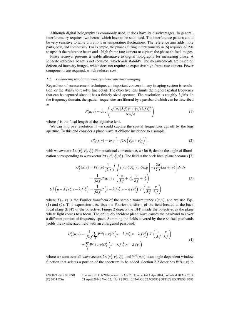
Regardless of measurement technique, an important concern in any imaging system is resolu-tion, or the ability to resolve fine detail. The objective lens limits the highest spatial frequencythat can be captured since it has a finitely sized aperture. The resolution is roughly λ/NA. Inthe frequency domain, the spatial frequencies are filtered by a passband which can be describedas
P(u,v) = circ
(√(u/(λ f ))2 +(v/(λ f ))2
NA/λ
)(1)
where f is the focal length of the objective lens.We can improve resolution if we could capture the spatial frequencies cut off by the lens
aperture. To this end consider a plane wave at oblique incidence to a sample,
Ukin(x,y) = exp
[− j2π
(vk
xx+ vkyy)]
, (2)
with wavevector 2π(vk
x,vky,v
kz). For notational convenience, we let θk denote the angle of illumi-
nation corresponding to wavevector 2π(vk
x,vky,v
kz). The field at the back focal plane becomes [7]
Ukf (u,v) = P(u,v)
1jλ f
∫ ∫t(x,y)Uk
in(x,y)exp[− j
2π
λ f(xu+ yv)
]dxdy
=1
jλ fP(u,v) T
(u
λ f+ vk
x,v
λ f+ vk
y
)Uk
f
(u−λ f vk
x,v−λ f vky
)=
1jλ f
P(
u−λ f vkx,v−λ f vk
y
)T(
uλ f
,v
λ f
) (3)
where T (u,v) is the Fourier transform of the sample transmittance t(x,y), and we use Eqs.(1) and (2). This expression describes the Fourier transform of the field located at the backfocal plane (BFP) of the objective. Figure 2 depicts the BFP inside the objective, as the planewhere light comes to a focus. The obliquely incident plane wave causes the passband to covera different portion of frequency space. Summing the fields covered by these shifted passbandsyields the synthesized field with an enlargened passband:
U sf (u,v) =
1jλ f ∑
kW k(u,v)P
(u−λ f vk
x,v−λ f vky
)T(
uλ f
,v
λ f
)= ∑
kW k(u,v)Uk
f
(u−λ f vk
x,v−λ f vky
) (4)
where we sum over all wavevectors 2π(vk
x,vky,v
kz), and W k(u,v) is an angle dependent window
function that selects a portion of the spectrum to be added. Section 2.2 describes W k(u,v) in
#206829 - $15.00 USD Received 20 Feb 2014; revised 3 Apr 2014; accepted 4 Apr 2014; published 10 Apr 2014(C) 2014 OSA 21 April 2014 | Vol. 22, No. 8 | DOI:10.1364/OE.22.009380 | OPTICS EXPRESS 9382
more detail. We note that taking a direct sum by omitting W k(u,v) is not entirely accurate,since a direct sum would place too much emphasis on the low frequencies and introduce phaseaberrations [12]. In effect we are synthetically increasing the numerical aperture of the lens. Forthis reason researchers refer to this technique as synthetic aperture imaging. As a consequence,the imaging system rejects out-of-focus diffraction noise. The resulting image looks cleaner,and techniques like numerical refocusing or differential interference contrast can be digitallyimplemented [6]. We note that another application, tomographic phase microscopy, also usesthe concept of illuminating the sample at oblique angles [13, 14], and it is a possible futureextension of this work.
2. Phase retrieval algorithm
2.1. General steps
Phase retrieval is a non-interferometric way of measuring phase. The basic idea is to measurea sequence of defocused intensity images I1, ..., IN at N planes and then process these imagesto extract the phase encoded in the defocus. There are different algorithms that process thesedefocused images to produce a phase image. Deterministic phase retrieval uses a closed formrelation between intensity and phase. Solving a Poisson-type equation yields phase [15–19].However, this equation relies on the paraxial approximation [15]. In our experiment, we illu-minate the sample at oblique angles with plane waves of the form in Eq. (2), which in generalwill not satisfy the paraxial approximation.
Another class of algorithms is iterative in nature. We can view the intensity measurements asconstraints, and we would like to retrieve a complex field satisfying those constraints [20, 21].We apply an iterative algorithm similar to the single beam multiple intensity reconstruction(SBMIR) technique [22–26]. The general steps are
1. In the first plane, let the complex amplitude U1 =√
I1 with a phase of φ1(x,y) = 0. Setn = 1.
2. Numerically propagate the complex amplitude at the previous plane Un to the next plane.Extract the phase φn+1(x,y).
3. Take the updated complex amplitude as Un+1 =√
In+1exp [ jφn+1(x,y)]. Increment n by1.
4. Go to step 2. Iterate until last plane is reached.
We can also add more iterations if desired. For example, the complex amplitude at the lastplane can be numerically propagated backwards using a similar update procedure. Conver-gence is checked by numerically propagating the retrieved field and comparing with measuredintensities. In our experiments, we measure a total of 15 planes, as described later in Section3, and we find that numerically propagating forward once and backward once through all theplanes is enough for convergence.
The above steps describe how to retrieve phase for one angle of illumination. The idea behindsynthetic aperture imaging is to measure phase at multiple angles of illumination. Our proposalis to implement synthetic aperture imaging using phase retrieval. For each angle of illumina-tion, we apply the above procedure to calculate phase. The combination of intensity and phasecompletely describes the complex field. Then the synthesized field is calculated by summingthe complex fields at each angle with the background phases set equal, as described by Eq. (4).The synthesized phase is the phase of the synthesized field.
#206829 - $15.00 USD Received 20 Feb 2014; revised 3 Apr 2014; accepted 4 Apr 2014; published 10 Apr 2014(C) 2014 OSA 21 April 2014 | Vol. 22, No. 8 | DOI:10.1364/OE.22.009380 | OPTICS EXPRESS 9383
(a) Partition of the synthesized spectrum intoquadrants.
(b) Partition of the synthesized spectrum into octants.
(c) 5 total angles scanned at the back focal planeof the condenser.
(d) 9 total angles scanned at the back focal planeof the condenser.
Fig. 1. Partition of the synthesized spectrum for aperture synthesis.
By implementing synthetic aperture imaging using phase retrieval, we hope to obtain a morecompact experimental setup that has fewer parts, smaller expenses, and more stability. To con-cisely describe this idea, we refer to it as synthetic aperture phase retrieval.
We summarize the synthetic aperture phase retrieval procedure as follows:
1. Select an angle θk.
2. Apply the iterative phase retrieval algorithm given above for a single angle. Retrieve thespectrum Uk
f (u,v) (Eq. (3)).
3. Go to step 1. Repeat until all angles are measured.
4. Sum the spectra Ukf (u,v) (Eq. (4)) to obtain U s
f (u,v).
5. Take the inverse Fourier transform of U sf (u,v) to obtain the synthesized field.
2.2. Stitching of the synthesized spectrum
Here we describe the angle dependent window function W k(u,v) from Eq. (4). A simple sum ofthe retrieved spectra from each angle of illumination would place too much weight on the lowfrequencies and introduce phase aberrations [12]. To avoid these effects, we filter the retrievedspectra with window functions W k(u,v). The intuition is that at each angle, the passband shiftsto cover a different part of the spectrum, as Eq. (3) describes. We would like to capture thegeneral part of the spectrum being measured for each angle. To implement this idea, we partitionthe synthesized spectrum into angular regions, according to the example presented in [12].
#206829 - $15.00 USD Received 20 Feb 2014; revised 3 Apr 2014; accepted 4 Apr 2014; published 10 Apr 2014(C) 2014 OSA 21 April 2014 | Vol. 22, No. 8 | DOI:10.1364/OE.22.009380 | OPTICS EXPRESS 9384
Figure 1 shows schematics of how the spectrum can be partitioned. Then the basic idea is tostitch together the synthesized spectrum from the retrieved spectra at each angle of illumination.We illustrate the procedure in the following examples.
Consider the example of measured spectra at 5 total angles. In our experiment we scan theback focal plane of the condenser lens (i.e., the focal plane to the left of the condenser lens, asdepicted in Fig. 2) to illuminate the sample at different angles; more details are given in Section3. For convenience, we number the beam positions at the back focal plane in Fig. 1(c). When thebeam is at position 0, we retrieve the DC or zero degree spectrum U0
f (u,v), using the notation ofEq. (3). At position 1, we retrieve the spectrum U1
f (u,v) of an obliquely illuminated sample. Themain lobe of U1
f (u,v) lies in quadrant 1 from Fig. 1(a). More generally, at position k, we retrievethe spectrum Uk
f (u,v) of the sample illuminated at angle θk, and the main lobe of Ukf (u,v)
lies in quadrant k. The synthesized spectrum is composed of selected parts of each spectrumUk
f (u,v). The central part of the synthesized spectrum (of radius approximately NA/λ ) consistsof U0
f (u,v). Outside the central part, quadrant k of the synthesized spectrum consists of Ukf (u,v).
The inverse Fourier transform of the synthesized spectrum yields the synthesized field.From the above description, we can better understand the factor W k(u,v) from Eq. (4). For
k = 0, W 0(u,v) is a circ function of radius approximately NA/λ , or
W 0(u,v) =
{1, if
√u2 + v2 < NA/λ ,
0, otherwise.(5)
For k > 0, W k(u,v) is zero everywhere except for a weight of 1 in quadrant k outside a radiusof approximately NA/λ , or
W k(u,v) =
{1, if (u,v) ∈ quadrant k and
√u2 + v2 > NA/λ ,
0, otherwise.(6)
In the case of measured spectra at 9 total angles, we number the beam positions at the backfocal plane of the condenser lens in Fig. 1(d). The octants in Fig. 1(b) are numbered similarly;octant 1 contains the positive u-axis, and octant 3 contains the positive v-axis (numbers are notshown in the figure because of space). When the beam is at position k, we retrieve Uk
f (u,v) forthe sample illuminated at angle θk, and the main lobe of Uk
f (u,v) lies in octant k. The centralpart of the synthesized spectrum (of radius approximately NA/λ ) consists of U0
f (u,v). Outsidethe central part, octant k of the synthesized spectrum consists of the following weighted sum:12
Ukf (u,v)+
14
Uk−1f (u,v)+
14
Uk+1f (u,v), where the indices k, k−1, and k+1 fall in the range
1, . . . ,8. Here we choose the spectrum retrieved at angle θk to have the largest weighting of1/2, while the spectra retrieved from neighboring angles have equal weightings of 1/4. Otherweightings can be chosen. Finally the inverse Fourier transform of the synthesized spectrumyields the synthesized field.
We can also describe W k(u,v) for this case of 9 total angles. For k = 0, Eq. (5) describesW 0(u,v). For k > 0, W k(u,v) is zero everywhere except for weights of 1/2 in octant k and 1/4in octants k−1 and k+1, all outside a radius of approximately NA/λ , or
W k(u,v) =
12 , if (u,v) ∈ octant k and
√u2 + v2 > NA/λ ,
14 , if (u,v) ∈ octant k−1 and
√u2 + v2 > NA/λ ,
14 , if (u,v) ∈ octant k+1 and
√u2 + v2 > NA/λ ,
0, otherwise,
(7)
#206829 - $15.00 USD Received 20 Feb 2014; revised 3 Apr 2014; accepted 4 Apr 2014; published 10 Apr 2014(C) 2014 OSA 21 April 2014 | Vol. 22, No. 8 | DOI:10.1364/OE.22.009380 | OPTICS EXPRESS 9385
Fig. 2. Experimental setup for synthetic aperture phase retrieval. M1: gimbal mount mirror;L1: lens (f = 300 mm); C: condenser lens (NA 1.25); OL: objective lens (NA 0.75); L2:tube lens (f = 200 mm).
where the indices k, k−1, and k+1 fall in the range 1, . . . ,8, as noted previously. To be fullyrigorous, the index k− 1 should be replaced with (k− 2) mod 8+ 1, so that when k = 1, theprevious index is 8. Similarly, the index k+1 should be replaced with k mod 8+1, so that whenk = 8, the next index is 1. However, for simplicity, we use the notation in Eq. (7).
3. Experimental setup
Figure 2 illustrates the experimental setup for synthetic aperture phase retrieval. A helium-neon(HeNe, λ = 633 nm) laser serves as the illumination source. Mirror M1 is a motorized gimbalmount, which operates under computer control. It steers the beam at different angles to provideoblique illumination at the sample. After traveling through the condenser lens (Abbe condenser,1.25 NA) and objective lens (50X, 0.75 NA), the beam is directed through a tube lens and ontoa CCD camera, which is mounted on a computer controlled translation stage. We measure asequence of intensity images by translating the camera along the axial direction. As the stagemoves, the images become defocused. From these defocused images, we apply the iterativephase retrieval algorithm to recover phase.
We note that our experiment uses a 0.75 NA objective; it can be extended to use the 1.4 NAin [6]. We also note that there are very high 1.65 NA objectives, but they require special highindex immersion oil that evaporates within a few hours and leaves a crystalline residue. Theyalso require special expensive and fragile coverslips [27]. In this work we aim to demonstratethe principle of using phase retrieval to implement synthetic aperture imaging. Our approachenables resolution enhancement without requiring an expensive high NA objective.
The experimental procedure is to first select an angle of illumination by tilting mirror M1.Then a sequence of defocused intensity images is measured by translating the camera. In ourexperiments, for each angle we measure 15 intensity images at planes separated by 2.1 µm,where 2.1 µm refers to the sample space, and the planes are symmetric about the focal planeat z = 0. We determine the focal plane to be the plane at which the samples look most trans-parent. More details on how to choose these parameters can be found in [22]. In Fig. 3, weshow 5 images for one of our samples, 10 µm polystyrene beads (n = 1.587) immersed in oil(n = 1.515). For a given angle of illumination, it takes about 7 seconds to record 15 intensityimages. We note that it should be possible to process these images in real time using a recentlydeveloped Kalman filtering algorithm [28]. We also note that electronically controllable, vari-able focus lenses can defocus the image in place of translating the camera, potentially speedingacquisition time [29].
#206829 - $15.00 USD Received 20 Feb 2014; revised 3 Apr 2014; accepted 4 Apr 2014; published 10 Apr 2014(C) 2014 OSA 21 April 2014 | Vol. 22, No. 8 | DOI:10.1364/OE.22.009380 | OPTICS EXPRESS 9386
(a) z = -6.3 µm. (b) z = -2.1 µm. (c) z = 0 µm.
(d) z = 2.1 µm. (e) z = 6.3 µm.
Fig. 3. Intensity images at zero degrees. Scale bar: 6 µm.
(a) 1 angle. (b) 5 total angles. (c) 9 total angles.
Fig. 4. Angular scanning at back focal plane of the condenser lens.
To provide oblique illumination at the sample, the beam scans the back focal plane of thecondenser lens, as illustrated in Fig. 4. To clarify, Fig. 2 depicts the back focal plane (BFP) ofthe condenser lens to the left of the condenser lens, as the plane where light comes to a focus.Thus Fig. 4 portrays focal spots at the BFP. Note at the sample, the beam stays centered andcollimated at all angles.
For nonzero degree illumination, the camera translation is no longer parallel to the beamdirection. As a result, the images move transversely as the camera moves axially. Consequentlythe images need to be registered. We perform this registration by creating an interference patternat the camera plane and measuring the beam angle from the fringes. The procedure is describedas follows. A beamsplitter taps off a reference beam before the sample. The sample beam is thebeam exiting the tube lens. Another beamsplitter combines the reference beam and the samplebeam to create an interference pattern at the camera. From the resulting fringes, the angle ofthe beam can be measured, and we use this angle to register our images. Note that we use theinterferometer only for calibration purposes. Once we measure the illumination angle for eachcontrol signal sent to tilt mirror M1, the interferometer can be removed from the setup. In Fig. 5we show 5 images taken at 12.3 degrees illumination for one of our samples, 10 µm polystyrenebeads, and these images are shown after being registered.
#206829 - $15.00 USD Received 20 Feb 2014; revised 3 Apr 2014; accepted 4 Apr 2014; published 10 Apr 2014(C) 2014 OSA 21 April 2014 | Vol. 22, No. 8 | DOI:10.1364/OE.22.009380 | OPTICS EXPRESS 9387
(a) z = -6.3 µm. (b) z = -2.1 µm. (c) z = 0 µm.
(d) z = 2.1 µm. (e) z = 6.3 µm.
Fig. 5. Intensity images at 12.3 degrees. Scale bar: 6 µm.
As an example of the angular scanning procedure, Fig. 4(b) depicts 4 angles measured aroundthe periphery of the back focal plane, in addition to zero degree illumination (the center dot). Inour current configuration, we can illuminate the sample at angles up to 12.3 degrees, measuredby the fringe analyis described earlier. We scan the periphery of the back focal plane in anapproximate circle so that the largest angle of illumination is 12.3 degrees.
4. Phase measurements
In this section we present two examples of phase measurements to highlight the reduction indiffraction noise and the enhancement of resolution enabled by synthetic aperture imaging. Thefirst experiment uses 10 µm polystyrene beads, both to illustrate our experimental procedurefrom Section 3 and to demonstrate reduction in diffraction noise. These beads have a clearlydefined circular shape, and we also show that aperture synthesis enhances this circular profile.In the second experiment, we image small (< 1 µm) dust particles on a glass slide. Due to thesmaller feature sizes, we obtain clearer evidence of resolution enhancement.
4.1. Experiment 1: Polystyrene beads
In our first experiment, we image 10 µm polystyrene beads (n = 1.587) immersed in oil(n = 1.515). The simplest case occurs when we only measure a phase image at zero de-gree illumination; in other words, we do not perform synthetic aperture imaging. We performphase retrieval at zero degrees according to the procedure described in Section 3. Figure 6shows the resulting phase image. We can roughly calculate the expected peak phase shift as∆φ = (2π/λ )∆z(nbead−nbkg) = 6.97 rad, where ∆z = 9.75µm according to the manufacturer’snominal specifications, nbead = 1.587, and nbkg = 1.515. We estimate the measured peak phaseshift by averaging the phase within the black circle in Fig. 6(b); the estimated shift is ∆φ = 6.42rad, which is reasonably close to the refractive index calculations. The phase retrieval algorithmoutputs wrapped phase, and to aid visualization, we also unwrap the results. For phase unwrap-ping we implement the algorithm presented in [30].
#206829 - $15.00 USD Received 20 Feb 2014; revised 3 Apr 2014; accepted 4 Apr 2014; published 10 Apr 2014(C) 2014 OSA 21 April 2014 | Vol. 22, No. 8 | DOI:10.1364/OE.22.009380 | OPTICS EXPRESS 9388
(a) Wrapped phase (rad). The dashed whiterectangle and circle will be used for noiseanalysis.
(b) Unwrapped phase (rad). Two dashed black cir-cles highlight spaces between the beads. The lowerdashed circle will be used for calculating averagephase.
Fig. 6. Test case 1: Phase image at 0 degrees. Scale bar: 6 µm.
(a) Wrapped phase (rad). (b) Unwrapped phase (rad). Two dashed black cir-cles highlight spaces between the beads. The lowerdashed circle will be used for calculating averagephase.
Fig. 7. Phase image from off-axis interferometry. Scale bar: 6 µm.
#206829 - $15.00 USD Received 20 Feb 2014; revised 3 Apr 2014; accepted 4 Apr 2014; published 10 Apr 2014(C) 2014 OSA 21 April 2014 | Vol. 22, No. 8 | DOI:10.1364/OE.22.009380 | OPTICS EXPRESS 9389
For reference, we also use off-axis interferometry to measure a phase image at zero degreeillumination. We tap off a portion of the input beam before the sample as a reference beam, asdescribed in Section 3. Figure 7 illustrates the off-axis results. We estimate the peak shift byaveraging the phase within the black circle in Fig. 7(b); the estimated peak shift is ∆φ = 7.57rad. However, the image is very noisy, so the phase values are not entirely accurate. Moreimportantly, this figure provides a comparison with the phase retrieval result in Fig. 6. In bothfigures, the circular profiles of the beads look jagged. In addition, the spaces between the beads,highlighed by dashed black circles in Figs. 6(b) and 7(b), appear partially blended with thebeads. We hope to enhance the circular profile of the beads and the resolution between thebeads by using synthetic aperture imaging.
We choose this sample of clumps of beads because it exhibits clear diffraction noise. Forexample, from the defocused intensity images in Fig. 3, we can see that the diffraction patternsfrom each individual bead interferes with those of other beads. Diffraction noise appears in Fig.6 as diffraction rings and speckle-like patterns inside the beads, which is most clearly seen inthe wrapped phase image. Similarly, we can discern some speckle-like patterns inside the beadsin Fig. 7. We hope to reduce this diffraction noise with synthetic aperture imaging.
Next we perform synthetic aperture imaging by illuminating the sample at multiple angles.We examine the synthesized phase images for the different numbers of angles listed in Table1. Figure 8 shows a phase image captured at 11.0 degrees illumination. To aid visualization,we also unwrap the phase. Although there are some unwrapping errors, the figure illustratesthe basic idea. We note that synthetic aperture imaging does not require phase unwrapping;the spectra are stitched together as described in Section 2.2. Since the beam is oblique to thecamera, the beads appear slightly elongated [6, 13]. As in the case of zero degree illumination,speckle-like patterns inside the beads and diffraction rings appear. To the best of our knowledge,this work is the first experimental demonstration of phase retrieval on an obliquely illuminatedsample.
#206829 - $15.00 USD Received 20 Feb 2014; revised 3 Apr 2014; accepted 4 Apr 2014; published 10 Apr 2014(C) 2014 OSA 21 April 2014 | Vol. 22, No. 8 | DOI:10.1364/OE.22.009380 | OPTICS EXPRESS 9390
(a) Wrapped phase (rad). The dashed whiterectangle and circle will be used for noiseanalysis.
(b) Unwrapped phase (rad). Two dashed black circleshighlight spaces between the beads.
Fig. 9. Test case 2: Synthesized phase image with 5 total angles. Scale bar: 6 µm.
(a) Wrapped phase (rad). The dashed whiterectangle and circle will be used for noiseanalysis.
(b) Unwrapped phase (rad). Two dashed black circleshighlight spaces between the beads.
Fig. 10. Test case 3: Synthesized phase image with 9 total angles. Scale bar: 6 µm.
For test case 2, we measure a total of 5 angles, as noted in Table 1. We perform syntheticaperture imaging by adding the angular spectra according to Eq. (4), together with the windowfunctions from Eqs. (5) and (6). The resulting synthesized phase is illustrated in Fig. 9. We seethat diffraction noise features, such as the diffraction rings and the speckle-like patterns insidethe beads, have been reduced compared to test case 1, which can be seen most clearly from thewrapped phase images.
For test case 3, we measure a total of 9 angles as noted in Table 1. The angular spectraare added according to Eq. (4), together with the window functions from Eqs. (5) and (7).Figure 10 shows the synthesized phase. The diffraction noise features (diffraction rings andspeckle-like patterns inside the beads) appear more reduced than test case 2. As more angles aremeasured, the passband in Eq. (1) shifts to cover different portions of frequency space, whichyields the different angular fields in Eq. (3). As a result, when these angular fields are summedin Eq. (4), the synthesized field contains an enlargened passband. Hence, we would expect this
#206829 - $15.00 USD Received 20 Feb 2014; revised 3 Apr 2014; accepted 4 Apr 2014; published 10 Apr 2014(C) 2014 OSA 21 April 2014 | Vol. 22, No. 8 | DOI:10.1364/OE.22.009380 | OPTICS EXPRESS 9391
Table 2. Phase speckle and background noise comparisons.Test Phase speckle % reduction in σ2
s Background % reduction in σ2b
case noise σ2s(rad2) compared to case 1 noise σ2
b
(rad2) compared to case 1
1 σ2s = 8.30×10⁻² 0% σ2
b = 1.75×10⁻² 0%2 σ2
s = 3.36×10⁻² 59% σ2b = 1.51×10⁻² 14%
3 σ2s = 1.49×10⁻² 82% σ2
b = 7.68×10⁻³ 56%
improvement in diffraction noise with more angles. In addition, the circular shape of the beadsbecomes progressively less jagged as more angles are measured, as Figs. 6(a), 9(a), and 10(a)show. We also notice the spaces between the beads become increasingly distinguishable as moreangles are added; these spaces are highlighted by dashed black circles in Figs. 6(b), 9(b), and10(b).
Next we examine a quantitative comparison of the DC case (test case 1) and the syn-thetic aperture cases (test cases 2 and 3). We measure the phase speckle noise σ2
s insidethe bead (dashed circle) for Fig. 6(a)
(σ2
s = 8.30×10⁻² rad2) and for Figs. 9(a) and 10(a)(σ2
s = 3.36×10⁻² and 1.49×10⁻² rad2 respectively); the phase speckle noise reduces by
59% and 82% respectively, compared to the DC case. We also measure the background noiseσ2
b inside the dashed rectangle for Fig. 6(a)(σ2
b = 1.75×10⁻² rad2) and for Figs. 9(a) and10(a)
(σ2
b = 1.51×10⁻² and 7.68×10⁻³ rad2 respectively); the background noise reduces by
14% and 56% respectively, compared to the DC case. Table 2 summarizes these results. We seethat adding more angles reduces the diffraction noise.
4.2. Experiment 2: Particles on a glass slide
In the second experiment, we image small (< 1 µm) dust particles on a glass slide. Similar tothe demonstration of resolution enhancement in [12], we examine particles that are close to theresolution limit of the imaging system, with the goal of showing better differentiation betweenparticles with aperture synthesis. A total of 9 angles are measured, and the retrieved spectrafrom each angle are added according to Eq. (4), together with the window functions from Eqs.(5) and (7).
To demonstrate resolution enhancement, we compare the DC or zero degree phase in Fig.11(a) with the synthesized phase in Fig. 11(b). In general, the synthesized phase looks sharper.We highlight two pairs of particles that are hard to distinguish with dashed white circles. Tofacilitate comparison, we plot line profiles along the lines shown in insets A and B. As the pro-files in Figs. 11(c) and 11(d) indicate, the synthesized phase shows increased contrast betweenthe two particles, allowing them to be better differentiated.
We can estimate the resolution of the setup from the line profiles in Fig. 11. In general, thespatial resolution is determined by the NA and wavelength as
δ =κλ
NA(8)
where the factor κ depends on experimental parameters such as the signal to noise ratio of thedetector [12]. For our experiment, λ = 633 nm and NA = 0.75. We estimate the resolution asδ = 1.59 µm from Fig. 11(c), where two particles look close to the resolution limit for the DCphase. Using aperture synthesis, we expect this resolution to improve to
δ =κλ
NA+ sinθillum(9)
#206829 - $15.00 USD Received 20 Feb 2014; revised 3 Apr 2014; accepted 4 Apr 2014; published 10 Apr 2014(C) 2014 OSA 21 April 2014 | Vol. 22, No. 8 | DOI:10.1364/OE.22.009380 | OPTICS EXPRESS 9392
(a) DC phase (rad). Scale bar: 6 µm.Inset scale bar: 1 µm.
(b) Synthesized phase (rad). Scale bar: 6 µm.Inset scale bar: 1 µm.
(c) Line profile from inset A. (d) Line profile from inset B.
Fig. 11. Resolution enhancement of particles on a glass slide.
where θillum is the angle of illumination used for the synthetic aperture. We take θillum = 12.3degrees, which is the largest angle of illumination for our experiment. From Eq. (9), we expectthe resolution to improve to δ = 1.24 µm. Indeed, Fig. 11(d) shows two particles separated by1.36 µm which become distinguishable after aperture synthesis.
We also measure the reduction in diffraction noise, as we did for the polystyrene beadsin Table 2. Inside the dashed white rectangles in Figs. 11(a) and 11(b), we calculate thebackground noise for the DC phase
(σ2
b = 2.05×10⁻² rad2) and the synthesized phase(σ2
b = 9.12×10⁻³ rad2); the background noise reduces by 55%. As a consequence, the diffrac-tion rings near the bottom of Fig. 11(a) disappear, enabling other particles to be better distin-guished.
5. Conclusion
We have demonstrated the principle of using phase retrieval to implement synthetic apertureimaging. Synthetic aperture imaging reduces diffraction noise and enhances resolution by effec-tively increasing the numerical aperture. Previously this technique has relied on digital hologra-phy for phase measurements. By obviating the need for a reference arm, this approach providesa more compact, less expensive, and more stable setup. Our demonstration paves the way for
#206829 - $15.00 USD Received 20 Feb 2014; revised 3 Apr 2014; accepted 4 Apr 2014; published 10 Apr 2014(C) 2014 OSA 21 April 2014 | Vol. 22, No. 8 | DOI:10.1364/OE.22.009380 | OPTICS EXPRESS 9393
other applications such as tomographic phase microscopy to be enabled by phase retrieval.
Acknowledgments
We thank Dr. Daniel E. Leaird for providing technical feedback and for machining parts to buildthe experiment. We are grateful to Jingjing Liu and Delong Zhang for help in acquiring andpreparing the test samples. We acknowledge the anonymous reviewers for their constructivecriticisms which improved the manuscript. In particular, we thank reviewer 2 for suggestingthe idea of stitching selected parts of the spectrum for aperture synthesis. We thank ProfessorJames Krogmeier, Dr. Alexei Lagoutchev, Joseph Lukens, A.J. Metcalf, Jian Wang, and Dr.Ping Wang for helpful discussions and suggestions. This work was supported in part by theNational Science Foundation under grant ECCS-1102110.
#206829 - $15.00 USD Received 20 Feb 2014; revised 3 Apr 2014; accepted 4 Apr 2014; published 10 Apr 2014(C) 2014 OSA 21 April 2014 | Vol. 22, No. 8 | DOI:10.1364/OE.22.009380 | OPTICS EXPRESS 9394