Optical solitons and other soluions forRadhakrishnan–Kundu–Lakshmanan equation inbirefringent bers by an ecient computationaltechniqueM. Bilal

Punjab University: Panjab UniversityMohammad Youins ( profdclu@hotmail.com )

Jiangsu UniversityAly Ramadan Seadawy

Cairo UniversityS.T.R. Rizvi

COMSATS University Islamabad

Research Article

Keywords: Optical soliton, RKL equation, Generalized exponential rational function method

Posted Date: April 12th, 2021

DOI: https://doi.org/10.21203/rs.3.rs-285910/v1

License: This work is licensed under a Creative Commons Attribution 4.0 International License. Read Full License

Version of Record: A version of this preprint was published at Optical and Quantum Electronics on July22nd, 2021. See the published version at https://doi.org/10.1007/s11082-021-03083-8.

Optical solitons and other soluions for

Radhakrishnan–Kundu–Lakshmanan equation in birefringent

fibers by an efficient computational technique

M. Bilal 1, M.Younis1, A.R. Seadawy2,3, S.T.R. Rizvi4

1PUCIT, University of the Punjab, Lahore 54000, Pakistan.

2 Mathematics Department, Faculty of science, Taibah University, Al-Madinah Al-Munawarah, Saudi Arabia.

3 Mathematics Department, Faculty of Science, Beni-Suef University, Beni Suef, Egypt.

4Department of Mathematics, COMSATS University Islamabad, Lahore Campus, Lahore Pakistan.

Abstract

In this article, we are interested to discuss the exact optical soiltons and other solutions in birefringent fibers

modeled by Radhakrishnan-Kundu-Lakshmanan equation in two component form for vector solitons. We extract

the solutions in the form of hyperbolic, trigonometric and exponential functions including solitary wave solutions

like multiple-optical soliton, mixed complex soliton solutions. The strategy that is used to explain the dynamics

of soliton is known as generalized exponential rational function method. Moreover, singular periodic wave solu-

tions are recovered and the constraint conditions for the existence of soliton solutions are also reported. Besides,

the physical action of the solution attained are recorded in terms of 3D, 2D and contour plots for distinct param-

eters. The achieved outcomes show that the applied computational strategy is direct, efficient, concise and can

be implemented in more complex phenomena with the assistant of symbolic computations. The primary benefit

of this technique is to develop a significant relationships between NLPDEs and others simple NLODEs and we

have succeeded in a single move to get and organize various types of new solutions. The obtained outcomes show

that the applied method is concise, direct, elementary and can be imposed in more complex phenomena with

the assistant of symbolic computations

keywords: Optical soliton, RKL equation, Generalized exponential rational function method

1 Introduction

In the science and technology fields like engineering, circuit analysis, fluid mechanics, solid state physics, chemical

physics, plasma physics, geochemistry, optical fiber, quantum field theory and biological sciences, NLPDEs are

used as a governing model to explain the complexity of the physical phenomena. To know the behaviour of intricate

physical phenomena, it is necessary to calculate the solutions of the governing NLPDEs. Generally, the solutions

of the NLPDEs are categorized into three types as exact solutions, analytic solutions and numerical solutions.

Finding the exact solutions of NLPDEs has the importance to discuss the stability of numerical solutions and also

development of a broad range of new scholar to simplify the routine calculation. Exact solutions to NLPDEs play

corresponding author: aly742001@yahoo.com

an important role in nonlinear science, since they can provide much physical information and more insight of the

physical aspects of the problem and thus lead to further applications. Wave phenomena in dispersion, dissipation,

diffusion, reaction and convection are very much important.

Furtehrmore, various specialists and mainstream researchers are giving more consideration to create and

improve the optical transmission frameworks through optical fibers instead of birefringent fibers. However, the

propagation of soliton through optical fibers governs next generation technology but there are several factors

in birefringent fibers as well that are used to produce the soliton propagations. It is polarization of light that

prompts bunch speed mismatch,which is at last liable for differential gathering delay and numerous other negative

impacts and consequently the examination of optical soliton is one of the most intriguing and interesting zones of

exploration in nonlinear optics. There are well known computational and powerful techniques to find the optical

exact soliton solutions of the differential equations [1–14].

Therefore, in this study we focus on constructing the exact optical soliton solutions in different structures to the

RKL equation for birefringent fibers without 4WM terms in media with Kerr-law nonlinearity which is known as

the basic case of fiber nonlinearity. Most optical fibers which has been quite popular recently comply with this law

nonlinearity. Also, this media indicates itself as self-phase modulation, a self-induced phase- and frequency-shift

of a pulse of light when it moves along with any fiber nonlinearity. In case of birefringent fibers the pulses are

polarized. Naturally, vector solitons are studied in birefringent fibers. We apply an efficent compuational approach

known as generlized exponential rational function method (GERFM) to find the various kinds of soliton solutions.

The restraint relations are also observed during the mathematical analysis.

The RKL with Kerr law nonlinearity is given below [15–19]

iΘt + αΘxx + β|Θ|2Θ = iλ(|Θ|2Θ)x − iδΘxxx, (1)

where the dependent variable Θ(x, t) is complex-valued wave profile with two independent variables of x and t that

represents spatio-temporal component, respectively. The first term characterizes temporal evolution whereas the

parameters α denotes group velocity dispersion (GVD) while, the coefficients β is Kerr nonlinearity. Moreover, on

right hand side the coefficients δ and λ sequentially accounts the third order dispersion (3OD) which induces soliton

radiation and the effect of self-steepening to eliminate the formulation of shock waves. Thus, these compensatory

effects of dispersion and nonlinearity provide the necessary balance to sustain soliton propagation.

Upon splitting the Eq. (1) for birefringent fibers into two components without 4WM [20], we arrive at:

iΨt + α1Ψxx + (β1|Ψ|2 + γ1|ϕ|2)Ψ = i

(

λ1(|Ψ|2Ψ)x + θ1(|ϕ|2Ψ)x

)

− iδ1Ψxxx (2)

iϕt + α2ϕxx + (β2|ϕ|2 + γ2|Ψ|2)ϕ = i

(

λ2(|ϕ|2ϕ)x + θ2(|Ψ|2ϕ)x)

− iδ2ϕxxx. (3)

The complex valued functions Ψ(x, t) and ϕ(x, t) represent the wave profiles and the Eq. (2) and Eq. (3) represent

the governing model for soliton transmission through birefringent fibers without 4WM . In the above coupled

system, the coefficient βj accounts for self-phase modulation (SPM) and the coefficient γj is the cross-phase

modulation terms respectively, for j = 1, 2. The coefficients λj and θj correspond to self-steepening terms, while

the the four-wave mixing effect is discarded.

This piece of article is discussed as sequence: In section 2, the summary of the GERFM. In section 3, optical

solitons. In section 4, results and discussion and finally paper comes at conclusions in section 5.

2 The summary of GERFM

Here, we give a brief description of GERFM [21]. Let us consider a nonlinear partial differential equation (PDE)

Ξ(u, ut, ux, utt, uxt, uxx, · · · ) = 0, (4)

where Ξ is a polynomial in its arguments.

The essence of GERFM can be presented in the following steps

Step 1. We introduce traveling wave transformation as:

u(x, t) = u(η) and η = B(x− ct),

where B and c represent the amplitude component and velocity respectively. After substituting this transformation

into Eq. (4), we get nonlinear ODE in the following form.

Υ(Λ,Λ′,Λ′′,Λ′′′, · · · ) = 0, (5)

where Υ is in general a polynomial function of its arguments and ′ denotes the derivative w.r.t η.

Step 2. Suppose that the solution of Eq. (5) can be expressed as follows

Λ(η) = d0 +

n∑

k=1

dkΩ(η)k +

n∑

k=1

fkΩ(η)−k, (6)

where

Ω(η) =r1e

s1η + r2es2η

r3es3η + r4es4η. (7)

The unknown coefficients d0, dk, fk (1 ≤ k ≤ n) and constants ri, si (1 ≤ i ≤ 4) are determined and the value of

n will be evaluated by using homogeneous balance principle.

Step 3. After putting Eq. (6) into Eq. (5) we get an algebraic equation R(η, es1η, es2η, es3η, es4η) = 0. Set-

ting each coefficient of R equal to zero, we get a system of nonlinear equations in the form of d0, dk, fk (1 ≤ k ≤ n)

and ri, si (1 ≤ i ≤ 4) is yielded.

Step 4. on solving the above system of equations we will get the values of d0, dk, fk (1 ≤ k ≤ n) and ri, si

(1 ≤ i ≤ 4) with the aid of any symbolic computation packages . Substituting these values in Eq. (6) we attain

the soliton solutions of Eq. (4).

3 Optical solitons

For solving the above couple system of Eqs. (2)-(3), we suppose the traveling wave transformation as follows:

Ψ(x, t) = Q1(η)eiψ, (8)

ϕ(x, t) = Q2(η)eiψ, (9)

where

η = B(x− νt) and ψ = −kx+ ωt+ θ0. (10)

And Qj(η) for (j = 1, 2), B, ν, θ0, ω and k represent the amplitude component of the soliton, velocity of soliton,

phase constant, soliton wave number and soliton frequency respectively. Substituting above transformations of

Eqs. (8)-(10) into Eqs. (2) and (3), we get real and imaginary parts, respectively of the form

B2(αj + 3kδj)Q′′

j − (ω + αjk2 + δjk

3)Qj + (βj − kλj)Q3j + γjQjQ

2j− kθjQjQ

2j= 0, (11)

B3δjQ′′′

j −B(ν + 2kαj + 3k2δj)Q′

j − 3BλjQ2j− θjBQ

′

jQ2j− 2θjBQjQjQ

′

j= 0. (12)

In order to use the balancing rule, the important results emerged from Eqs. (11)-(12) by using of Qj = Qj are

B2(αj + 3kδj)Q′′

j − (ω + αjk2 + δjk

3)Qj + (βj − kλj + γj − kθj)Q3j = 0, (13)

B2δjQ′′

j − (ν + 2kαj + 3k2δj)Qj − (λj + θj)Q3j = 0. (14)

We can obtain

ω =8k3δ2j + 8k2αjδj + 3kνδj + 2kα2

j + ναj

δj, (15)

βj = −2kδjθj + 2kδjλj + αjθj + αjλj + δjγj

δj, (16)

which yields from

αj + 3kδjδj

=ω + αjk

2 + δjk3

ν + 2kαj + 3k2δj= −βj − kλj + γj − kθj

λj + θj. (17)

As the function Qj satisfies Eqs. (13)-(14). We will use Eq. (13) with Eqs. (15)-(16).

By balancing the highest order derivative and nonlinear term appear in Eq. (13) we attain n = 1. Using n = 1

along with Eqs. (6)-(7), then

Qj(η) = d0 + d1Ω(η) + f1Ω(η)−1. (18)

Family-1: If we take r = [−1,−1, 1,−1] and s = [1,−1, 1,−1], then Eq. (7) changes into

Ω(η) = −cosh(η)

sinh(η). (19)

Case-1:

d0 = 0, d1 = 0, f1 = −√

k3 (−δj)− k2αj − ω√

−βj − γj + kθj + kλj, B =

√

k3 (−δj)− k2αj − ω√2√

αj + 3kδj.

Inserting these values in Eqs. (18) and (19), then we obtain

The optical dark soliton solution as

Ψ(x, t) =

√

k3 (−δ1)− k2α1 − ω√−β1 − γ1 + kθ1 + kλ1

tanh

[

√

k3 (−δ1)− k2α1 − ω√2√α1 + 3kδ1

(x− νt)

]

×ei(−kx+8k

3δ21+8k

2α1δ1+3kδ1+2kα

21+να1

δ1t+θ0), (20)

ϕ(x, t) =

√

k3 (−δ2)− k2α2 − ω√−β2 − γ2 + kθ2 + kλ2

tanh

[

√

k3 (−δ2)− k2α2 − ω√2√α2 + 3kδ2

(x− νt)

]

×ei(−kx+8k

3δ22+8k

2α2δ2+3kδ2+2kα

22+να2

δ2t+θ0). (21)

Here (k3 (−δj) − k2αj − ω)(αj + 3kδj) > 0 and δj 6= 0 with j = 1, 2 for valid solution. The graphical

representations of the solutions are shown for different values of parameters.

(a)

(b)

(c)

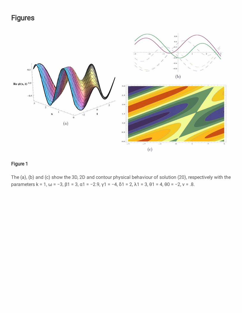
Figure 1: The (a), (b) and (c) show the 3D, 2D and contour physical behaviour of solution (20), respectively withthe parameters k = 1, ω = −3, β1 = 3, α1 = −2.9, γ1 = −4, δ1 = 2, λ1 = 3, θ1 = 4, θ0 = −2, ν = .8.

(a)

(b)

(c)

Figure 2: The (a), (b) and (c) show the 3D, 2D and contour physical behaviour of solution (21), respectively withthe parameters k = 1, ω = −4, β2 = 1, α2 = −2, γ2 = −4.6, δ2 = 3, λ2 = 7, θ2 = −3, θ0 = −1, ν = .3.

Case 2:

d0 = 0, d1 =

√

k3 (−δj)− k2αj − ω√

−βj − γj + kθj + kλj, f1 = 0, B =

√

k3 (−δj)− k2αj − ω√2√

αj + 3kδj.

Substituting these values in Eqs. (18) and (19), we attain

The singular optical soliton solution as

Ψ(x, t) = −√

k3 (−δ1)− k2α1 − ω√−β1 − γ1 + kθ1 + kλ1

coth

[

√

k3 (−δ1)− k2α1 − ω√2√α1 + 3kδ1

(x− νt)

]

×ei(−kx+8k

3δ21+8k

2α1δ1+3kδ1+2kα

21+να1

δ1t+θ0), (22)

ϕ(x, t) = −√

k3 (−δ2)− k2α2 − ω√−β2 − γ2 + kθ2 + kλ2

coth

[

√

k3 (−δ2)− k2α2 − ω√2√α2 + 3kδ2

(x− νt)

]

×ei(−kx+8k

3δ22+8k

2α2δ2+3kδ2+2kα

22+να2

δ2t+θ0). (23)

Here (k3 (−δj) − k2αj − ω)(αj + 3kδj) > 0 and δj 6= 0 with j = 1, 2 for valid solution. The graphical repre-

sentations of the solutions are shown for different values of parameters.

(a)

(b)

(c)

Figure 3: The (a), (b) and (c) show the 3D, 2D and contour physical behaviour of solution (22), respectively withthe parameters k = 1, ω = −6, β1 = 1, α1 = −4, γ1 = −2, δ1 = 3, λ1 = 2, θ1 = 6, θ0 = −1, ν = .7.

(a)

(b)

(c)

Figure 4: The (a), (b) and (c) show the 3D, 2D and contour physical behaviour of solution (23), respectively withthe parameters k = 1, ω = −3.6, β2 = 2, α2 = −3, γ2 = −5, δ2 = 4, λ2 = 8, θ2 = −2, θ0 = −3, ν = .3.

Case-3:

d0 = 0, d1 =

√

k2 (αj + kδj) + ω√

−2βj − 2γj + 2k (θj + λj), f1 = −

√

k2 (αj + kδj) + ω√

−2βj − 2γj + 2k (θj + λj),

B =

√

k2 (αj + kδj) + ω

2√

αj + 3kδj.

Imposing these values in Eqs. (18) and (19), then we derive

The combined optical soliton solution as

Ψ(x, t) = −√

k2 (α1 + kδ1) + ω√

−2β1 − 2γ1 + 2k (θ1 + λ1)

1

sinh

[√k2(α1+kδ1)+ω

2√α1+3kδ1

(x− νt)

]

cosh

[√k2(α1+kδ1)+ω

2√α1+3kδ1

(x− νt)

]

×ei(−kx+8k

3δ21+8k

2α1δ1+3kδ1+2kα

21+να1

δ1t+θ0), (24)

ϕ(x, t) = −√

k2 (α2 + kδ2) + ω√

−2β2 − 2γ2 + 2k (θ2 + λ2)

1

sinh

[√k2(α2+kδ2)+ω

2√α2+3kδ2

(x− νt)

]

cosh

[√k2(α2+kδ2)+ω

2√α2+3kδ2

(x− νt)

]

×ei(−kx+8k

3δ22+8k

2α2δ2+3kδ2+2kα

22+να2

δ2t+θ0). (25)

Here (k2 (αj + kδj) + ω)(αj + 3kδj) > 0 and δj 6= 0 with j = 1, 2 for valid solution. The graphical represen-

tations of the solutions are shown for different values of parameters.

(a)

(b)

(c)

Figure 5: The (a), (b) and (c) show the 3D, 2D and contour physical behaviour of solution (24), respectively withthe parameters k = 2, ω = 5, β1 = .5, α1 = 1, γ1 = −5, δ1 = 7, λ1 = 3, θ1 = 5, θ0 = −3, ν = 2.

(a)

(b)

(c)

Figure 6: The (a), (b) and (c) show the 3D, 2D and contour physical behaviour of solution (25), respectively withthe parameters k = 2, ω = 1, β2 = −3, α2 = 4, γ2 = 0, δ2 = 5, λ2 = 6, θ2 = 7, θ0 = 2, ν = 1.5.

Family-2: If we chose r = [−i,−i, 1, 1] and s = [i,−i, i,−i], then Eq. (7) modify into

Ω(η) = − sin(η)

cos(η). (26)

The following trigonometric and combined trigonometric traveling wave solutions are

Case-1:

d0 = 0, d1 = 0, f1 = −√

k3δj + k2αj + ω√

−βj − γj + kθj + kλj, B =

√

k3δj + k2αj + ω√2√

αj + 3kδj.

Substituting these values in Eqs. (18) and (26), we attain

Ψ(x, t) =

√k3δ1 + k2α1 + ω√

−β1 − γ1 + kθ1 + kλ1cot

[√k3δ1 + k2α1 + ω√2√α1 + 3kδ1

(x− νt)

]

×ei(−kx+8k

3δ21+8k

2α1δ1+3kδ1+2kα

21+να1

δ1t+θ0), (27)

ϕ(x, t) =

√k3δ2 + k2α2 + ω√

−β2 − γ2 + kθ2 + kλ2cot

[√k3δ2 + k2α2 + ω√2√α2 + 3kδ2

(x− νt)

]

×ei(−kx+8k

3δ22+8k

2α2δ2+3kδ2+2kα

22+να2

δ2t+θ0). (28)

Here ((

k3δj + k2αj)

+ ω)(αj + 3kδj) > 0 and δj 6= 0 with j = 1, 2 for valid solution. The graphical represen-

tations of the solutions are shown for different values of parameters.

(a)

(b)

(c)

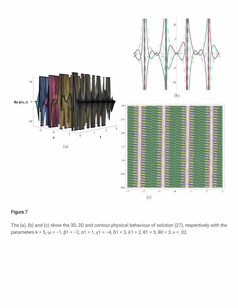
Figure 7: The (a), (b) and (c) show the 3D, 2D and contour physical behaviour of solution (27), respectively withthe parameters k = 5, ω = −1, β1 = −2, α1 = 1, γ1 = −4, δ1 = 3, λ1 = 2, θ1 = 5, θ0 = 3, ν = .02.

(a)

(b)

(c)

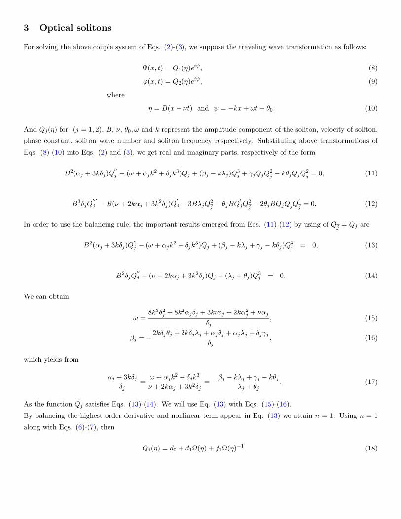
Figure 8: The (a), (b) and (c) show the 3D, 2D and contour physical behaviour of solution (28), respectively withthe parameters k = 4, ω = 3, β2 = 0, α2 = 3, γ2 = 0, δ2 = 8, λ2 = 2, θ2 = 3, θ0 = 3, ν = .3.

Case-2:

d0 = 0, d1 = −√

k3δj + k2αj + ω√

−βj − γj + kθj + kλj, f1 = 0, B =

√

k3δj + k2αj + ω√2√

αj + 3kδj.

Replacing these values in Eqs. (18) and (26), we get

Ψ(x, t) =

√k3δ1 + k2α1 + ω√

−β1 − γ1 + kθ1 + kλ1tan

[√k3δ1 + k2α1 + ω√2√α1 + 3kδ1

(x− νt)

]

×ei(−kx+8k

3δ21+8k

2α1δ1+3kδ1+2kα

21+να1

δ1t+θ0), (29)

ϕ(x, t) =

√k3δ2 + k2α2 + ω√

−β2 − γ2 + kθ2 + kλ2tan

[√k3δ2 + k2α2 + ω√2√α2 + 3kδ2

(x− νt)

]

×ei(−kx+8k

3δ22+8k

2α2δ2+3kδ2+2kα

22+να2

δ2t+θ0). (30)

Here ((

k3δj + k2αj)

+ ω)(αj + 3kδj) > 0 and δj 6= 0 with j = 1, 2 for valid solution. Case-3:

d0 = 0, d1 = −√

k2 (αj + kδj) + ω

2√

−βj − γj + k (θj + λj), f1 =

√

k2 (αj + kδj) + ω

2√

−βj − γj + k (θj + λj), B =

√

k2 (αj + kδj) + ω

2√2√

αj + 3kδj.

Inserting these values in Eqs. (18) and (26), we obtained

Ψ(x, t) =

√

k2 (α1 + kδ1) + ω

2√

−β1 − γ1 + k (θ1 + λ1)

1− 2 cos2[√

k2(α1+kδ1)+ω

2√2√α1+3kδ1

(x− νt)

]

sin

[√k2(α1+kδ1)+ω

2√2√α1+3kδ1

(x− νt)

]

cos

[√k2(α1+kδ1)+ω

2√2√α1+3kδ1

(x− νt)

]

×ei(−kx+8k

3δ21+8k

2α1δ1+3kδ1+2kα

21+να1

δ1t+θ0), (31)

ϕ(x, t) =

√

k2 (α2 + kδ2) + ω

2√

−β2 − γ2 + k (θ2 + λ2)

1− 2 cos2[√

k2(α2+kδ2)+ω

2√2√α2+3kδ2

(x− νt)

]

sin

[√k2(α2+kδ2)+ω

2√2√α2+3kδ2

(x− νt)

]

cos

[√k2(α2+kδ2)+ω

2√2√α2+3kδ2

(x− νt)

]

×ei(−kx+8k

3δ22+8k

2α2δ2+3kδ2+2kα

22+να2

δ2t+θ0). (32)

Here (k2 (αj + kδj) + ω)(αj + 3kδj) > 0 and δj 6= 0 with j = 1, 2 for valid solution.

Family-3: If we take r = [2, 1, 1, 1] and s = [1, 0, 1, 0], then Eq. (7) transform into

Ω(η) =2eη + 1

eη + 1. (33)

Case-1:

d0 =3√

k2 (− (αj + kδj))− ω√

−βj − γj + k (θj + λj), d1 = −2

√

k2 (− (αj + kδj))− ω√

−βj − γj + k (θj + λj), f1 = 0,

B =

√2√

k2 (− (αj + kδj))− ω√

αj + 3kδj.

Inserting these values in Eqs. (18) and (33), then

The exponential function solution can be expressed as

Ψ(x, t) =

(

√

k2 (− (α1 + kδ1))− ω√

−β1 − γ1 + k (θ1 + λ1)

1− eη

eη + 1

)

ei(−kx+

8k3δ21+8k

2α1δ1+3kδ1+2kα

21+να1

δ1t+θ0), (34)

where η =√2√k2(−(α1+kδ1))−ω√

α1+3kδ1(x− νt).

ϕ(x, t) =

(

√

k2 (− (α2 + kδ2))− ω√

−β2 − γ2 + k (θ2 + λ2)

1− eη

eη + 1

)

ei(−kx+

8k3δ22+8k

2α2δ2+3kδ2+2kα

22+να2

δ2t+θ0), (35)

where η =√2√k2(−(α2+kδ2))−ω√

α2+3kδ2(x− νt).

Here (k2 (− (αj + kδj)) − ω)(−βj − γj + k (θj + λj)) > 0 and δj 6= 0 with j = 1, 2 for valid solution. The

graphical representations of the solutions are shown for different values of parameters.

(a)

(b)

(c)

Figure 9: The (a), (b) and (c) show the 3D, 2D and contour physical behaviour of solution (34), respectively withthe parameters k = 0, ω = −1, β1 = −2, α1 = 1, γ1 = 0, δ1 = −3, λ1 = 5, θ1 = 4, θ0 = 2, ν = 3.

(a)

(b)

(c)

Figure 10: The (a), (b) and (c) show the 3D, 2D and contour physical behaviour of solution (35), respectivelywith the parameters k = 1, ω = −4, β2 = −2, α2 = 0, γ2 = −5, δ2 = −2, λ2 = 3, θ2 = 4, θ0 = 2, ν = 1.

Case-2:

d0 = −3√

k2 (− (αj + kδj))− ω√

−βj − γj + k (θj + λj), d1 = 0, f1 =

4√

k2 (− (αj + kδj))− ω√

−βj − γj + k (θj + λj),

B =

√2√

k2 (− (αj + kδj))− ω√

αj + 3kδj.

Putting these values in Eqs. (18) and (33), then

The exponential function solution can be formulated as

Ψ(x, t) =

(

√

k2 (− (α1 + kδ1))− ω√

−β1 − γ1 + k (θ1 + λ1)

1− 2eη

2eη + 1

)

ei(−kx+

8k3δ21+8k

2α1δ1+3kδ1+2kα

21+να1

δ1t+θ0), (36)

where η =√2√k2(−(α1+kδ1))−ω√

α1+3kδ1(x− νt).

ϕ(x, t) =

(

√

k2 (− (α2 + kδ2))− ω√

−β2 − γ2 + k (θ2 + λ2)

1− 2eη

2eη + 1

)

ei(−kx+

8k3δ22+8k

2α2δ2+3kδ2+2kα

22+να2

δ2t+θ0), (37)

where η =√2√k2(−(α2+kδ2))−ω√

α2+3kδ2(x− νt).

Here (k2 (− (αj + kδj))− ω)(−βj − γj + k (θj + λj)) > 0 and δj 6= 0 with j = 1, 2 for valid solution.

Family-4: If we take r = [1− i, 1 + i,−1, 1] and s = [i,−i, i,−i], then Eq. (7) convert into

Ω(η) =cos(η) + sin(η)

cos(η). (38)

Case-1:

d0 =

√

k2 (αj + kδj) + ω√

−βj − γj + k (θj + λj), d1 = −

√

k2 (αj + kδj) + ω√

−βj − γj + k (θj + λj), f1 = 0, B =

√

k2 (αj + kδj) + ω√2√

αj + 3kδj.

Imposing these values in Eqs. (18) and (38), then

The singular periodic wave solution can be expressed as

Ψ(x, t) = −√

k2 (α1 + kδ1) + ω√

−β1 − γ1 + k (θ1 + λ1)tan

[

√

k2 (α1 + kδ1) + ω√2√α1 + 3kδ1

(x− νt)

]

×ei(−kx+8k

3δ21+8k

2α1δ1+3kδ1+2kα

21+να1

δ1t+θ0), (39)

ϕ(x, t) = −√

k2 (α2 + kδ2) + ω√

−β2 − γ2 + k (θ2 + λ2)tan

[

√

k2 (α2 + kδ2) + ω√2√α2 + 3kδ2

(x− νt)

]

×ei(−kx+8k

3δ22+8k

2α2δ2+3kδ2+2kα

22+να2

δ2t+θ0). (40)

Here (k2 (αj + kδj) + ω)(αj + 3kδj) > 0 and δj 6= 0 with j = 1, 2 for valid solution.

Case-2:

d0 =

√

k2 (αj + kδj) + ω√

−βj − γj + k (θj + λj), d1 = 0, f1 = − 2

√

k2 (αj + kδj) + ω√

−βj − γj + k (θj + λj), B =

√

k3δj + k2αj + ω√

2αj + 6kδj.

Inserting these values in Eqs. (18) and (38), then

The combined singular periodic wave solution can be written as

Ψ(x, t) =

√

k2 (α1 + kδ1) + ω√

−β1 − γ1 + k (θ1 + λ1)

(sin[

√k3δ1+k2α1+ω√2α1+6kδ1

(x− νt)]− cos[

√k3δ1+k2α1+ω√2α1+6kδ1

(x− νt)]

cos[

√k3δ1+k2α1+ω√2α1+6kδ1

(x− νt)] + sin[

√k3δ1+k2α1+ω√2α1+6kδ1

(x− νt)]

)

×ei(−kx+8k

3δ21+8k

2α1δ1+3kδ1+2kα

21+να1

δ1t+θ0), (41)

ϕ(x, t) =

√

k2 (α2 + kδ2) + ω√

−β2 − γ2 + k (θ2 + λ2)

(sin[

√k3δ2+k2α2+ω√2α2+6kδ2

(x− νt)]− cos[

√k3δ2+k2α2+ω√2α2+6kδ2

(x− νt)]

cos[

√k3δ2+k2α2+ω√2α2+6kδ2

(x− νt)] + sin[

√k3δ2+k2α2+ω√2α2+6kδ2

(x− νt)]

)

×ei(−kx+8k

3δ22+8k

2α2δ2+3kδ2+2kα

22+να2

δ2t+θ0). (42)

Here ((

k2αj + k3δj)

+ ω)(2αj + 6kδj) > 0 and δj 6= 0 with j = 1, 2 for valid solution.

Family-5: If we take r = [−3,−1, 1, 1] and s = [1,−1, 1,−1], then Eq. (7) converts into

Ω(η) =−2 cosh(η)− sinh(η)

cosh(η)(43)

Case-1:

d0 = −2√

k2 (− (αj + kδj))− ω√

−βj − γj + k (θj + λj), d1 = −

√

k2 (− (αj + kδj))− ω√

−βj − γj + k (θj + λj), f1 = 0,

B =

√

k2 (− (αj + kδj))− ω√2√

αj + 3kδj.

Replacing these values in Eqs. (18) and (43), then

The hyperbolic function solution can be derived as

Ψ(x, t) =

√

k2 (− (α1 + kδ1))− ω√

−β1 − γ1 + k (θ1 + λ1)tanh

[

√

k2 (− (α1 + kδ1))− ω√2√α1 + 3kδ1

(x− νt)

]

×ei(−kx+8k

3δ21+8k

2α1δ1+3kδ1+2kα

21+να1

δ1t+θ0), (44)

ϕ(x, t) =

√

k2 (− (α2 + kδ2))− ω√

−β2 − γ2 + k (θ2 + λ2)tanh

[

√

k2 (− (α2 + kδ2))− ω√2√α2 + 3kδ2

(x− νt)

]

×ei(−kx+8k

3δ22+8k

2α2δ2+3kδ2+2kα

22+να2

δ2t+θ0). (45)

Here (k2(− (αj + kδj))− ω)(αj + 3kδj) > 0 and δj 6= 0 with j = 1, 2 for valid solution.

Case-2:

d0 = −2√

k2 (− (αj + kδj))− ω√

−βj − γj + k (θj + λj), d1 = 0, f1 = −3

√

k2 (− (αj + kδj))− ω√

−βj − γj + k (θj + λj),

B =

√

k2 (− (αj + kδj))− ω√2√

αj + 3kδj.

Substituting these values in Eqs. (18) and (43), then

The mixed hyperbolic function solution can be formulated as

Ψ(x, t) = −√

k2 (− (α1 + kδ1))− ω√

−β1 − γ1 + k (θ1 + λ1)

(2 sinh[

√k2(−(α1+kδ1))−ω√

2√α1+3kδ1

(x− νt)] + cosh[

√k2(−(α1+kδ1))−ω√

2√α1+3kδ1

(x− νt)]

2 cosh[

√k2(−(α1+kδ1))−ω√

2√α1+3kδ1

(x− νt)] + sinh[

√k2(−(α1+kδ1))−ω√

2√α1+3kδ1

(x− νt)]

)

×ei(−kx+8k

3δ21+8k

2α1δ1+3kδ1+2kα

21+να1

δ1t+θ0), (46)

ϕ(x, t) = −√

k2 (− (α2 + kδ2))− ω√

−β2 − γ2 + k (θ2 + λ2)

(2 sinh[

√k2(−(α2+kδ2))−ω√

2√α2+3kδ2

(x− νt)] + cosh[

√k2(−(α2+kδ2))−ω√

2√α2+3kδ2

(x− νt)]

2 cosh[

√k2(−(α2+kδ2))−ω√

2√α2+3kδ2

(x− νt)] + sinh[

√k2(−(α2+kδ2))−ω√

2√α2+3kδ2

(x− νt)]

)

×ei(−kx+8k

3δ22+8k

2α2δ2+3kδ2+2kα

22+να2

δ2t+θ0), (47)

Here (k2(− (αj + kδj))− ω)(αj + 3kδj) > 0 and δj 6= 0 with j = 1, 2 for valid solution.

Family-6: If we take r = [−1, 0, 1, 1] and s = [0, 1, 0, 1], then Eq. (7) transform into

Ω(η) = − 1

eη + 1. (48)

Case-1:

d0 =

√

k3 (−δj)− k2αj − ω√

−βj − γj + kθj + kλj, d1 =

2√

k3 (−δj)− k2αj − ω√

−βj − γj + kθj + kλj, f1 = 0, B =

√2√

k3 (−δj)− k2αj − ω√

αj + 3kδj.

Inserting these values in Eqs. (18) and (48), then

The exponential function solution can be shown as

Ψ(x, t) =

(

√

k3 (−δ1)− k2α1 − ω√−β1 − γ1 + kθ1 + kλ1

eη − 1

1 + eη

)

ei(−kx+

8k3δ21+8k

2α1δ1+3kδ1+2kα

21+να1

δ1t+θ0), (49)

where η =√2√k3(−δ1)−k2α1−ω√α1+3kδ1

(x− νt).

ϕ(x, t) =

(

√

k3 (−δ2)− k2α2 − ω√−β2 − γ2 + kθ2 + kλ2

eη − 1

1 + eη

)

ei(−kx+

8k3δ22+8k

2α2δ2+3kδ2+2kα

22+να2

δ2t+θ0), (50)

where η =√2√k3(−δ2)−k2α2−ω√α2+3kδ2

(x− νt).

Here (k3 (−δj)− k2αj − ω)(−βj − γj + k (θj + λj)) > 0 and δj 6= 0 with j = 1, 2 for valid solution.

Family-7: If we take r = [−1, 1, 1, 1] and s = [1,−1, 1,−1], then Eq. (7) transform into

Ω(η) = − sinh(η)

cosh(η)(51)

Case-1:

d0 = 0, d1 =

√

k2 (− (αj + kδj))− ω

2√

−βj − γj + k (θj + λj), f1 =

√

k2 (− (αj + kδj))− ω

2√

−βj − γj + k (θj + λj), B =

√

k2 (− (αj + kδj))− ω

2√2√

−αj − 3kδj.

Inserting these values in Eqs. (18) and (51), then

The combo optical soliton solution can be transformed as

Ψ(x, t) = −√

k2 (− (α1 + kδ1))− ω

2√

−β1 − γ1 + k (θ1 + λ1)

( 2 cosh2[

√k2(−(α1+kδ1))−ω

2√2√−α1−3kδ1

(x− νt)]− 1

cosh[

√k2(−(α1+kδ1))−ω

2√2√−α1−3kδ1

(x− νt)] sinh[

√k2(−(α1+kδ1))−ω

2√2√−α1−3kδ1

(x− νt)]

)

×ei(−kx+8k

3δ21+8k

2α1δ1+3kδ1+2kα

21+να1

δ1t+θ0), (52)

ϕ(x, t) = −√

k2 (− (α2 + kδ2))− ω

2√

−β2 − γ2 + k (θ2 + λ2)

( 2 cosh2[

√k2(−(α2+kδ2))−ω

2√2√−α2−3kδ2

(x− νt)]− 1

cosh[

√k2(−(α2+kδ2))−ω

2√2√−α2−3kδ2

(x− νt)] sinh[

√k2(−(α2+kδ2))−ω

2√2√−α2−3kδ2

(x− νt)]

)

×ei(−kx+8k

3δ22+8k

2α2δ2+3kδ2+2kα

22+να2

δ2t+θ0). (53)

Here (k2(− (αj + kδj))− ω)(−αj − 3kδj) > 0 and δj 6= 0 with j = 1, 2 for valid solution.

Case-2:

d0 = 0, d1 = −√

k2 (− (αj + kδj))− ω

2√

−βj − γj + k (θj + λj), f1 = −

√

k2 (− (αj + kδj))− ω

2√

−βj − γj + k (θj + λj),

B =

√

k2 (− (αj + kδj))− ω

2√2√

−αj − 3kδj.

Substituting these values in Eqs. (18) and (51), then

The mixed optical soliton solution can be derived as

Ψ(x, t) = −√

k2 (− (α1 + kδ1))− ω

2√

−β1 − γ1 + k (θ1 + λ1)

( 2 sinh2[

√k2(−(α1+kδ1))−ω

2√2√−α1−3kδ1

(x− νt)] + 1

cosh[

√k2(−(α1+kδ1))−ω

2√2√−α1−3kδ1

(x− νt)] sinh[

√k2(−(α1+kδ1))−ω

2√2√−α1−3kδ1

(x− νt)]

)

×ei(−kx+8k

3δ21+8k

2α1δ1+3kδ1+2kα

21+να1

δ1t+θ0), (54)

ϕ(x, t) = −√

k2 (− (α2 + kδ2))− ω

2√

−β2 − γ2 + k (θ2 + λ2)

( 2 cosh2[

√k2(−(α2+kδ2))−ω

2√2√−α2−3kδ2

(x− νt)]− 1

cosh[

√k2(−(α2+kδ2))−ω

2√2√−α2−3kδ2

(x− νt)] sinh[

√k2(−(α2+kδ2))−ω

2√2√−α2−3kδ2

(x− νt)]

)

×ei(−kx+8k

3δ22+8k

2α2δ2+3kδ2+2kα

22+να2

δ2t+θ0). (55)

Here (k2(− (αj + kδj)) − ω)(−αj − 3kδj) > 0 and δj 6= 0 with j = 1, 2 for valid solution. The graphical

representations of the solutions are shown for different values of parameters.

(a)

(b)

(c)

Figure 11: The (a), (b) and (c) show the 3D, 2D and contour physical behaviour of solution (54), respectivelywith the parameters k = 8, ω = −2, β1 = −3, α1 = −6, γ1 = −5, δ1 = −4, λ1 = 4, θ1 = 0, θ0 = 1, ν = 1.5.

(a)

(b)

(c)

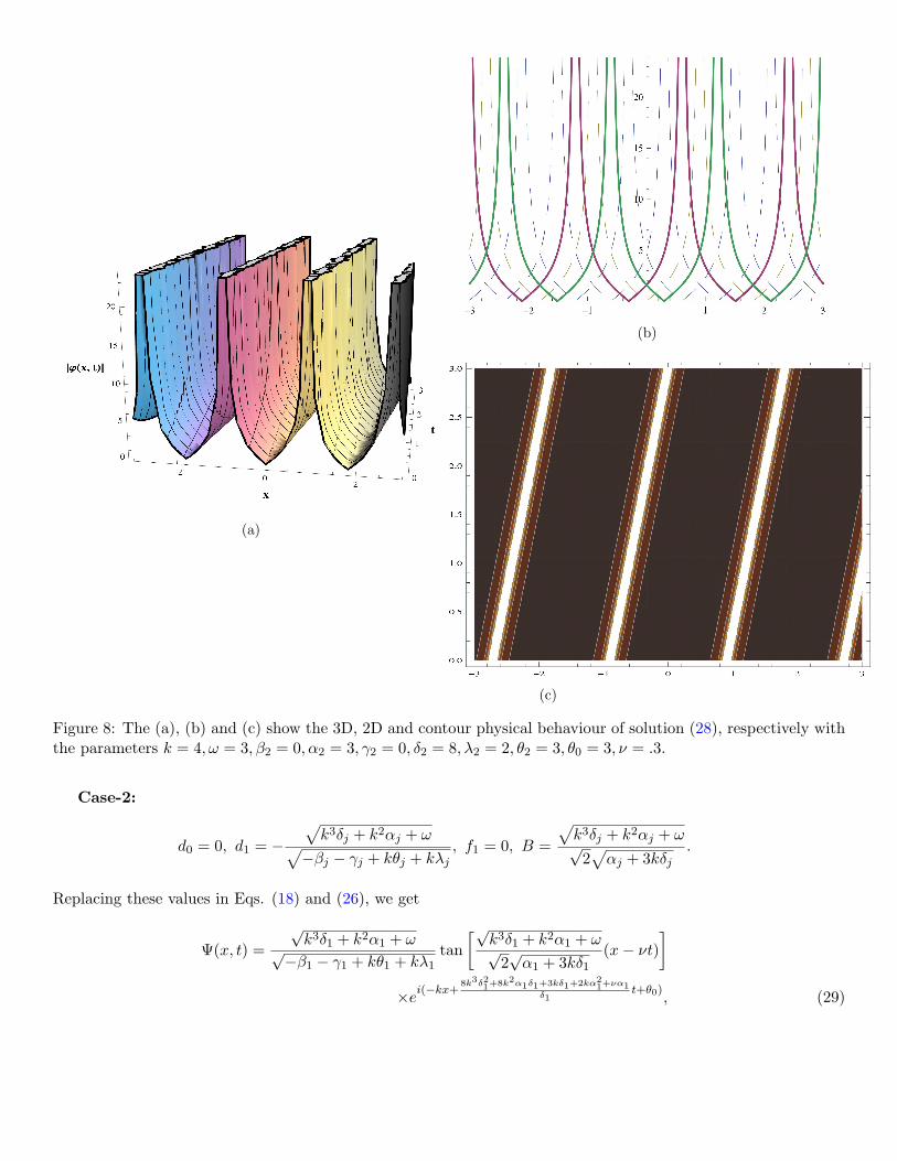
Figure 12: The (a), (b) and (c) show the 3D, 2D and contour physical behaviour of solution (55), respectivelywith the parameters k = 0, ω = −4, β2 = −5, α2 = −2, γ2 = −2, δ2 = −2, λ2 = 3, θ2 = 1, θ0 = 0, ν = 1.

Family-8: If we take r = [1, 2, 1, 1] and s = [1, 0, 1, 0], then Eq. (7) converts into

Ω(η) =eη + 2

eη + 1. (56)

Case-1:

d0 = −3√

k2 (− (αj + kδj))− ω√

−βj − γj + k (θj + λj), d1 = 0, f1 =

4√

k2 (− (αj + kδj))− ω√

−βj − γj + k (θj + λj),

B =

√2√

k2 (− (αj + kδj))− ω√

αj + 3kδj.

Insert these values in Eqs. (18) and (56), then

The solitary wave solution can be written as

Ψ(x, t) =

[

√

k2 (− (α1 + kδ1))− ω√

−β1 − γ1 + k (θ1 + λ1)

eη − 2

eη + 2

]

ei(−kx+

8k3δ21+8k

2α1δ1+3kδ1+2kα

21+να1

δ1t+θ0), (57)

where η =√2√k2(−(α1+kδ1))−ω√

α1+3kδ1(x− νt).

ϕ(x, t) =

[

√

k2 (− (α2 + kδ2))− ω√

−β2 − γ2 + k (θ2 + λ2)

eη − 2

eη + 2

]

ei(−kx+

8k3δ22+8k

2α2δ2+3kδ2+2kα

22+να2

δ2t+θ0), (58)

where η =√2√k2(−(α2+kδ2))−ω√

α2+3kδ2(x− νt).

Here (k2(− (αj + kδj))− ω)(−βj − γj + k (θj + λj)) > 0 and δj 6= 0 with j = 1, 2 for valid solution.

Case-2:

d0 = −3√

k2 (− (αj + kδj))− ω√

−βj − γj + k (θj + λj), d1 =

2√

k2 (− (αj + kδj))− ω√

−βj − γj + k (θj + λj), f1 = 0,

B =

√2√

k2 (− (αj + kδj))− ω√

αj + 3kδj.

Replacing these values in Eqs. (18) and (56), then

The solitary wave solution can be obtained as

Ψ(x, t) =

(

√

k2 (− (α1 + kδ1))− ω√

−β1 − γ1 + k (θ1 + λ1)

1− eη

1 + eη

)

ei(−kx+

8k3δ21+8k

2α1δ1+3kδ1+2kα

21+να1

δ1t+θ0), (59)

where η =√2√k2(−(α1+kδ1))−ω√

α1+3kδ1(x− νt).

ϕ =

(

√

k2 (− (α2 + kδ2))− ω√

−β2 − γ2 + k (θ2 + λ2)

1− eη

1 + eη

)

ei(−kx+

8k3δ22+8k

2α2δ2+3kδ2+2kα

22+να2

δ2t+θ0), (60)

where η =√2√k2(−(α2+kδ2))−ω√

α2+3kδ2(x− νt).

Here (k2(− (αj + kδj))− ω)(−βj − γj + k (θj + λj)) > 0 and δj 6= 0 with j = 1, 2 for valid solution.

4 Results and discussion

The results of this paper will be beneficial for learners to analyze the most attractive applications of the RKL

equation, which describes the prorogation of waves without 4WM in birefringent fibers. Figures 1-12 clearly

demonstrates the surfaces of the solution obtained for 3D, 2D and the contour plots, with choices of parameters

for the RKL model. We can capture the behaviour of the of the acquired solution with the assistant of contour

plots. In the same way, 3D figures tell us to model and demonstrate accurate physical behaviour. Through this

study, we consider the exact optical soliton solutions to the nonlinear RKL model using generalized exponential

rational function approach. The authors proposed different analytic approach in newly issued article and reported

some fascinating findings. We can grasp from all the graphs that the GERFM is very efficient and more precise

in evaluating the equation under consideration.

5 Conclusions

This paper extracted the dynamics of optical solitons in the RKL equation without 4WM in birefringent fibers.

The solutions are achieved in the shape of exponential, trigonometric and hyperbolic functions as well as exact

optical soliton solutions by the mechanism of GERFM under different constraint conditions which provide the

guaranty and validity of solutions are also listed. In addition, we attained the singular periodic wave solutions.

The model must be extended to govern DWDM networks so that parallel communication of soliton dynamics can

be addressed. These new families of solutions are shown the power, effectiveness and fruitfulness of this method.

This article shelters the application of optical fibers. Also, these fresh solutions have many applications in physics

and other branches of physical sciences.

References

[1] B. Younas, M. Younis, Chirped solitons in optical monomode fibres modelled with Chen–Lee–Liu equation,

Pramana – J. Phys. 94, 3 (2020). https://doi.org/10.1007/s12043-019-1872-6

[2] A.R. Seadawy, M. Arshad, D. Lu, Dispersive optical solitary wave solutions of strain wave equation in micro-

structured solids and its applications, Physica A: Statistical Mechanics and its Applications, 540 (2020)

123122.

[3] M. Younis, M, Bilal, S.Rehman, U. Younas, S.T.R. Rizvi, Investigation of optical solitons in birefringent

polarization preserving fibers with four-wave mixing effect. Int. J. Mod. Phys. B, (2020) 2050113.

[4] G.D. Donne, M.B. Hubert, A.R. Seadawy, T. Etienne, G. Betchewe, S.Y. Doka, Chirped soliton solutions of

Fokas–Lenells equation with perturbation terms and the effect of spatio-temporal dispersion in the modula-

tional instability analysis, The European Physical Journal Plus, 135 (2) (2020) 212.

[5] M. Younis, U. Younas, S.U. Rehman, M. Bilal, A. Waheed, Optical bright-dark and Gaussian soliton with

third order dispersion, Optik 134 (2017) 233–238.

[6] H.U. Rehman, M.S. Saleem, M. Zubair, S. Jafar, I. Latif, Optical solitons with Biswas-Arshed model using

mapping method, Optik 194 (2019) 163091.

[7] M. Iqbal, A.R. Seadawy, D. Lu, X. Xianwe, Construction of a weakly nonlinear dispersion solitary wave

solution for the Zakharov–Kuznetsov-modified equal width dynamical equation, Indian Journal of Physics,

(2019) 1-10.

[8] M.S. Osman, K.U. Tariq, A. Bekir, A. Elmoasry, N.S. Elazab, M. Younis, Investigation of soliton solutions

with different wave structures to the (2+ 1)-dimensional Heisenberg ferromagnetic spin chain equation, Com-

munications in Theoretical Physics 72 (3) (2020) 035002.

[9] M. Younis, T.A. Sulaiman, M. Bilal, S.U. Rehman, U. Younas, Modulation instability analysis, optical and

other solutions to the modified nonlinear Schrodinger equation, Communications in Theoretical Physics, 72

(2020) 065001 (12pp).

[10] D. Lu, A.R. Seadawy, I. Ahmed, Peregrine-like rational solitons and their interaction with kink wave for the

resonance nonlinear Schrodinger equation with Kerr law of nonlinearity, Modern Physics Letters B, 33 (24)

(2019) 1950292.

[11] A.R. Seadawy, A. Abdullah, Nonlinear complex physical models: optical soliton solutions of the complex

Hirota dynamical model, Indian Journal of Physics, (2019) 1-10.

[12] A.R. Seadawy, M. Arshad, D. Lu, Modulation stability analysis and solitary wave solutions of nonlinear

higher-order Schrodinger dynamical equation with second-order spatiotemporal dispersion, Indian Journal of

Physics, 93 (8) (2019) 1041-1049.

[13] M. Iqbal, A.R. Seadawy, O.H. Khalil, D. Lu, Propagation of long internal waves in density stratified ocean for

the (2+ 1)-dimensional nonlinear Nizhnik-Novikov-Vesselov dynamical equation, Results in Physics 16 (2020)

102838.

[14] M. Iqbal, A.R. Seadawy, D. Lu, X. Xia, Construction of bright–dark solitons and ion-acoustic solitary wave

solutions of dynamical system of nonlinear wave propagation, Modern Physics Letters A, 34 (37) (2019)

1950309.

[15] A. Biswas, Y. Yildirim, E. Yasar, M. F. Mahmood, A. S. Alshomrani, Q. Zhou, S. P. Moshokoa, M. Belic,

Optical soliton perturbation for Radhakrishnan–Kundu–Lakshmanan equation with a couple of integration

schemes, Optik. 163 (2018) 126–136.

[16] N.A. Kudryashov, D.V. Safonova, A. Biswas, Painleve analysis and a solution to the traveling wave reduction

of the Radhakrishnan–Kundu–Lakshmanan equation, Regul Chaotic Dyn. 24 (2019) 607-614.

[17] H.U. Rehman, M.S. Saleem, A.M. Sultan, M. Iftikhar, Comments on ”Dynamics of optical solitons with

Radhakrishnan–Kundu–Lakshmanan model via two reliable integration schemes, Optik 178 (2019) 557–566.

[18] T.A. Sulaiman, H. Bulut, G. Yel, S.S. Atas, Optical solitons to the fractional perturbed Radhakrishnan–

Kundu–Lakshmanan model, Opt. Quant. Electron. 50 (2018) 372. https://doi.org/10.1007/s11082-018-1641-

7.

[19] B. Sturdevant, D.A. Lott, A. Biswas, Topological 1-soliton solution of the generalized Radhakrishnan,

Kundu, Lakshmanan equation with nonlinear dispersion, Mod. Phys. Lett. B. 24 (2010) 1825–1831.

https://doi.org/10.1142/S0217984910024109.

[20] Y. Yıldırım, A. Biswas, M. Ekici, H. Triki, O. Gonzalez-Gaxiolah, A.K Alzahranic, M.R. Belici, Optical

solitons in birefringent fibers for Radhakrishnan–Kundu–Lakshmanan equation with five prolific integration

norms, Optik 208 (2020) 164550.

[21] B. Ghanbari, M. Inc, A.i Yusuf, D. Baleanu, New solitary wave solutions and stability analysis of the Benney-

Luke and the Phi-4 equations in mathematical physics, AIMS Mathematics, 4(6) (2019) 1523–1539.

Figures

Figure 1

The (a), (b) and (c) show the 3D, 2D and contour physical behaviour of solution (20), respectively with theparameters k = 1, ω = −3, β1 = 3, α1 = −2.9, γ1 = −4, δ1 = 2, λ1 = 3, θ1 = 4, θ0 = −2, ν = .8.

Figure 2

The (a), (b) and (c) show the 3D, 2D and contour physical behaviour of solution (21), respectively with theparameters k = 1, ω = −4, β2 = 1, α2 = −2, γ2 = −4.6, δ2 = 3, λ2 = 7, θ2 = −3, θ0 = −1, ν = .3.

Figure 3

The (a), (b) and (c) show the 3D, 2D and contour physical behaviour of solution (22), respectively with theparameters k = 1, ω = −6, β1 = 1, α1 = −4, γ1 = −2, δ1 = 3, λ1 = 2, θ1 = 6, θ0 = −1, ν = .7.

Figure 4

The (a), (b) and (c) show the 3D, 2D and contour physical behaviour of solution (23), respectively with theparameters k = 1, ω = −3.6, β2 = 2, α2 = −3, γ2 = −5, δ2 = 4, λ2 = 8, θ2 = −2, θ0 = −3, ν = .3.

Figure 5

The (a), (b) and (c) show the 3D, 2D and contour physical behaviour of solution (24), respectively with theparameters k = 2, ω = 5, β1 = .5, α1 = 1, γ1 = −5, δ1 = 7, λ1 = 3, θ1 = 5, θ0 = −3, ν = 2.

Figure 6

The (a), (b) and (c) show the 3D, 2D and contour physical behaviour of solution (25), respectively with theparameters k = 2, ω = 1, β2 = −3, α2 = 4, γ2 = 0, δ2 = 5, λ2 = 6, θ2 = 7, θ0 = 2, ν = 1.5.

Figure 7

The (a), (b) and (c) show the 3D, 2D and contour physical behaviour of solution (27), respectively with theparameters k = 5, ω = −1, β1 = −2, α1 = 1, γ1 = −4, δ1 = 3, λ1 = 2, θ1 = 5, θ0 = 3, ν = .02.

Figure 8

The (a), (b) and (c) show the 3D, 2D and contour physical behaviour of solution (28), respectively with theparameters k = 4, ω = 3, β2 = 0, α2 = 3, γ2 = 0, δ2 = 8, λ2 = 2, θ2 = 3, θ0 = 3, ν = .3.

Figure 9

The (a), (b) and (c) show the 3D, 2D and contour physical behaviour of solution (34), respectively with theparameters k = 0, ω = −1, β1 = −2, α1 = 1, γ1 = 0, δ1 = −3, λ1 = 5, θ1 = 4, θ0 = 2, ν = 3.

Figure 10

The (a), (b) and (c) show the 3D, 2D and contour physical behaviour of solution (35), respectively with theparameters k = 1, ω = −4, β2 = −2, α2 = 0, γ2 = −5, δ2 = −2, λ2 = 3, θ2 = 4, θ0 = 2, ν = 1.

Figure 11

The (a), (b) and (c) show the 3D, 2D and contour physical behaviour of solution (54), respectively with theparameters k = 8, ω = −2, β1 = −3, α1 = −6, γ1 = −5, δ1 = −4, λ1 = 4, θ1 = 0, θ0 = 1, ν = 1.5.

Figure 12

The (a), (b) and (c) show the 3D, 2D and contour physical behaviour of solution (55), respectively with theparameters k = 0, ω = −4, β2 = −5, α2 = −2, γ2 = −2, δ2 = −2, λ2 = 3, θ2 = 1, θ0 = 0, ν = 1.