Optimal Allocation to Hedge Funds : An Empirical Analysis Jaksa Cvitani´c, Ali Lazrak, Lionel Martellini and Fernando Zapatero ∗ November 25, 2002 Abstract What percentage of their portfolio should investors allocate to hedge funds? The only available answers to the above question are set in a static mean-variance framework, with no explicit accounting for uncertainty on the active manager’s ability to generate abnormal return, and usually generate unreasonably high allocations to hedge funds. In this paper, we apply the model introduced in Cvitani´c, Lazrak, Martellini and Zapatero (2002b) for optimal investment strategies in the presence of uncertain abnormal returns to a database of hedge funds. We find that the presence of model risk significantly decreases an investor’s optimal allocation to hedge funds. Another finding of this paper is that low beta hedge funds may serve as natural substitutes for a significant portion of an investor risk-free asset holdings. ∗ Jaksa Cvitanic is with the Departments of Mathematics and Economics at the University of Southern California. His research is supported in part by NSF grant DMS-00-99549. Ali Lazrak is with the Finance Department at the University of British Columbia. Lionel Martellini and Fernando Zapatero are with the Marshall School of Business at the University of Southern California. The author for correspondence is Lionel Martellini. He can be reached at University of Southern California, Marshall School of Business, Business and Economics, Hoffman Hall 710, Los Angeles, CA 90089-1427. Phone: (213) 740 5796. Email address: [email protected]. We would like to express our gratitude to Noël Amenc, Avi Bick, Marc Cassano, Nicole El Karoui, Robert Grauer, Alan Kraus, Gordon Sick as well as seminar participants at Calgary, SFU and UBC for very useful comments and suggestions. All errors are, of course, the authors’ sole responsibility. 1
Transcript
Optimal Allocation to Hedge Funds : AnEmpirical Analysis
Jaksa Cvitanic, Ali Lazrak, Lionel Martellini and Fernando Zapatero∗
November 25, 2002
Abstract
What percentage of their portfolio should investors allocate to hedge funds? The
only available answers to the above question are set in a static mean-variance framework,
with no explicit accounting for uncertainty on the active manager’s ability to generate
abnormal return, and usually generate unreasonably high allocations to hedge funds. In
this paper, we apply the model introduced in Cvitanic, Lazrak, Martellini and Zapatero
(2002b) for optimal investment strategies in the presence of uncertain abnormal returns
to a database of hedge funds. We find that the presence of model risk significantly
decreases an investor’s optimal allocation to hedge funds. Another finding of this paper
is that low beta hedge funds may serve as natural substitutes for a significant portion of
an investor risk-free asset holdings.
∗Jaksa Cvitanic is with the Departments of Mathematics and Economics at the University of SouthernCalifornia. His research is supported in part by NSF grant DMS-00-99549. Ali Lazrak is with the FinanceDepartment at the University of British Columbia. Lionel Martellini and Fernando Zapatero are with theMarshall School of Business at the University of Southern California. The author for correspondence is LionelMartellini. He can be reached at University of Southern California, Marshall School of Business, Business
and Economics, Hoffman Hall 710, Los Angeles, CA 90089-1427. Phone: (213) 740 5796. Email address:[email protected]. We would like to express our gratitude to Noël Amenc, Avi Bick, Marc Cassano, Nicole ElKaroui, Robert Grauer, Alan Kraus, Gordon Sick as well as seminar participants at Calgary, SFU and UBCfor very useful comments and suggestions. All errors are, of course, the authors’ sole responsibility.
1
1 Introduction
One of the by-products of the bull market of the 90’s has been the consolidation of hedge
funds as an important segment of financial markets. The value of the hedge fund industry
worldwide is estimated at more than 500 billion dollars distributed among over 5,000 hedge
funds.1 The majority of institutional investors seems to be moving towards holding hedge
funds in their portfolios.2 There seem to be two main reasons behind the success of hedge
funds (see Amenc, Curtis and Martellini (2001) and Schneeweis and Spurgin (1999) for a
detailed study). On the one hand, hedge funds seem to provide diversification with respect
to other existing investment possibilities (beta benefit). On the other hand, it is argued that
hedge funds provide an abnormal return adjusted by risk (alpha benefit).
In a nutshell, the diversification argument states that most hedge funds have a low beta with
respect to traditional stock and bond indexes. This is reported for example in Schneeweis and
Spurgin (1999, 2000) and Agarwal and Naik (2001), at least for some hedge fund strategies (the
so-called “non directional strategies”).3 The reason is that hedge funds can take advantage of
shortselling and include derivatives and other non-traditional asset classes in a way that is not
allowed to mutual funds. The second argument says that the alpha of hedge funds is positive.
There is a growing literature on the measurement of hedge fund risk-adjusted performance. We
mention here Ackermann, McEnally, and Ravenscraft (1999), Agarwal and Naik (2000a, 2000b,
2001), Amenc, Curtis and Martellini (2001), Amin and Kat (2001), Bares, Gibson and Gyger
(2001), Brown and Goetzmann (1997, 2001), Brown, Goetzmann, and Ibbotson (1999), Brown,
Goetzmann and Park (1997), Edwards and Liew (1999), Fung and Hsieh (1997a, 1997b, 2000),
Lhabitant (2001)) Liang (2000, 2001), Schneeweis and Spurgin (1999, 2000) and Schneeweis,
Spurgin and McCarthy (1996). Although these studies differ in the data and models they use
and their results are not completely homogeneous, most of them conclude that there is some
evidence of abnormal performance, at least in some segments of the hedge fund industry.
A standard way to present the benefits of hedge fund investing is to show the improvement
they allow for in a mean-variance analysis. For example, Schneeweis and Spurgin (1999)
construct a mean-variance frontier with the S&P500, the Lehman Brothers Bond Index and
a hedge fund index, the EACM 100.4 The conclusion of this study is that the inclusion of
hedge funds greatly improves the mean-variance frontier of investment possibilities. In fact,
1Frank Russell-Goldman Sachs survey (1999).2According to the Gollin, Harris, Ludgate (2001) survey, 64% of the European institutions included in the
study invest in hedge funds. This is up from 56% in 2000.3Agarwal and Naik (2001) report evidence of higher correlation between hedge fund returns and equity
market returns in bear markets as opposed to bull markets. This suggests that conditional betas tend to behigher than unconditional betas.
4The EACM 100 is, arguably, the most widely used index for the performance of hedge funds. For moreinformation on this index and an overview of existing hedge fund indices, see Amenc and Martellini (2002b).
2
the in-sample Sharpe ratio of hedge funds seems to be so superior to the Sharpe ratios of the
two other funds considered in this paper that the optimal investment strategy of an investor
that uses mean-variance analysis should be to invest almost all the risky part of the portfolio
in hedge funds. We view this normative prescription of an almost exclusive investment in
hedge funds as evidence of the failure of in-sample static mean-variance analysis to generate a
reasonable asset allocation including both traditional and alternative investment vehicles.5
Although the existing literature seems to grant the interest of hedge funds as valuable
investment alternatives, there seems to be several other shortcomings in the presentation of
the advantages of including hedge funds in an investor’s asset allocation. On one hand, as
it is clear from the arguments presented above, the analysis is in general cast in a mean-
variance setting. This is very restrictive because of all the well known assumptions on the
preferences of the investors and/or returns of the securities that are necessary in order to
make this setting appropriate. Furthermore, the analysis is static and rules out the possibility
of non-myopic behavior. On the other hand, this analysis relies heavily on good estimates
of expected returns. This problem seems to be far from solved (see Britten-Jones (1999)).
A related issue is the difficulty of measuring the alphas of hedge funds. Amenc, Curtis and
Martellini (2001) estimate alphas across several models and conclude that their quantification
varies greatly with the different models.
What percentage of their portfolio should investors allocate to alternative investment vehi-
cles given their low betas and uncertain potential for positive alphas? In this paper we apply
the model developed and analyzed in Cvitanic, Lazrak, Martellini and Zapatero (2002a,b) to
a database of hedge funds. Hedge fund offers some superior performance measured by its al-
pha. In the model we use, a non-myopic investor with incomplete information allocates wealth
between a riskfree security, a passive portfolio and an actively managed portfolio. A related
paper is Baks, Metrick and Wachter (2001). They test a model of actively managed funds with
heterogeneous priors about the alphas. However, investors in that model maximize quadratic
utilities: the hedging component of the investment strategy of the investor in our paper is
a key factor of the investment decision. Also, we use a different database for our test.6 An
important finding of this paper is that low beta hedge funds may serve as natural substitutes
for a significant portion of an investor risk-free asset holdings.
The paper is organized as follows. In the next section we present the model and optimal
investment strategy of an investor with incomplete information. In section 3, we present the
data, and perform the calibration of the model and derive empirical results in section 4. We
close the paper with some conclusions. Some information on hedge fund strategies can be
5Amenc and Martellini (2002a) perform out-of-sample testing of an improved asset return covariance matrixestimate and hedge fund allocation decisions.
6We focus on hedge funds while Baks, Metrick and Wachter (2001) focus on mutual funds.
3
found in a dedicated appendix.
2 Optimal Investment with Uncertain Alphas
In this section we briefly present the model and optimal investment strategy. The details,
derivation and comparative statics can be found in Cvitanic, Lazrak, Martellini and Zapatero
(2002b).
2.1 The Model
Uncertainty about risky asset prices in the economy is represented by a standard filtered
probability space (Ω,F ,F,P), on which is defined a 2-dimensional Brownian motion W =
(W 1,W 2). We assume that the investor can choose among three assets, a risk-free asset Bt,
and two risky assets. The first of them has a price that we denote by Pt and we interpret it
as a passive fund, a fund that tracks a broad-based index such as the S&P500, that is a proxy
for the market portfolio. The second security, whose price we denote by At, is a hedge fund.
The dynamics of the price of these assets are given by
dBt = Btrdt
dPt = Pt
¡eµPdt+ σPdW1t
¢dAt = At
¡eµAdt+ σ1dW1t + σ2dW
2t
¢where the invertible volatility matrix σ =
ÃσP 0
σ1 σ2
!as well as the interest rate r are assumed
to be constant. Alternatively, we could rewrite the dynamics of the prices as depending in a
single Brownian motion each, but with correlation ρ = σ1√σ21+σ
22
and volatility of the active fund
σA :=pσ21 + σ22. The previous notation allows simpler representation and interpretation of
the optimal investment strategy. We focus on lognormal processes, although the model can
in principle be solved for more general processes with stochastically time-varying drift and
volatilities.7
In this setting, there is a risk averse investor with initial wealth X0 who has access to
the three securities described above and that maximizes utility of final wealth, given by the
expression
u(XT ) =(XT )
a
a(1)
For a = 0 this would be logarithmic -myopic- utility. We focus in the more interesting case
a < 0.7There is evidence of departure from normality in hedge fund returns (Agarwal and Naik (2000), Fung and
Hsieh (1997a, 2000), Amin and Kat (2001) or Lo (2001)).
4
We assume that the investor does not observe neither the constant mean returns vectoreµ = (eµ1, eµ2) nor the source of noise W but observes the price processes (P,A). Therefore the
investor’s information consists of the P−augmentation of the filtration
Ft := σ(P (s), A(s); 0 ≤ s ≤ t)
generated by the price process (P (t), A(t)); t ∈ [0, T ]. Define the “risk premium” vectorprocess
θ(t) := σ−1(t)[eµ(t)− r(t)1]
where 1 = (1, 1) ∈ R2. In other words, θ = (θP , θA) with
θP =eµP − r
σP
θA = − σ1σPσ2
(eµP − r) +eµA − r
σ2
We assume that vector θ has a normal prior distribution
θ ∼ NÃφ =
ÃφPφA
!,∆ =
ÃδP 0
0 δA
!!with mean vector φ and variance-covariance matrix ∆ and we assume that θ is independent
of W . Here we assume that the priors are independent, as can be seen from the fact that the
off-diagonal terms in ∆ are zero. In Cvitanic, Lazrak, Martellini and Zapatero (2002b) we
consider the general case of correlated priors.
As explained in the introduction, the growth of hedge funds is partially motivated by
the possibility of risk-adjusted abnormal returns. With that motivation in mind, we further
specify the dynamics of the active portfolio. In particular, we decompose the drift of the active
portfolio into the sum of two elements, a normal return component and an abnormal return
component, or
eµA = r + β (eµP − r)| z normal return
+ eα|zabnormal return
(2)
where β = σ1σPσ2P
= σ1σPis the standard beta of the active fund with respect to the passive fund,
regarded as a broad-based index, a proxy for the market portfolio (the S&P500 in the empirical
tests of the model). Therefore, in order to measure risk-adjusted abnormal returns we use the
CAPM framework.8
8We do not assume that CAPM holds, but merely use its terminology.
5
2.1.1 Optimal Allocation to Hedge Funds
We assume that the investor considers the assets with prices P and A as possible investment
vehicles, with uncorrelated priors on their expected returns mP and mA, respectively. The
following proposition provides a simple expression for the optimal holding in the passive and
active portfolios.
Proposition 1 Under assumptions and notation specified in section 1, in the uncorrelatedcase (γ = 0), the optimal holdings in the active and passive portfolios can be expressed in the
following form
πA(0) =α0
σ22 (1− a− aδAT )(3)
πP (0) =mp − r
σ2P (1− a− aδPT )− βπA(0) (4)
where α0 = mA − r − β (mP − r) is the date 0 expected value of the abnormal return alpha of
the active fund for the investor with incomplete information, σ2 =qσ2A − β2σ2P is the residual,
or specific, component in the volatility of the active portfolio, and mP (resp. mA) is the prior
on the passive (resp. active) portfolio expected return.
P roof. See Cvitanic, Lazrak, Martellini and Zapatero (2002b).As expected, an increase in the expected alpha leads the investor to hold more of the active
portfolio, everything else equal. On the other hand, an increase in the uncertainty around
alpha leads the investor to hold less (or short less) of the active portfolio, everything else
equal.9 An increase in the time-horizon also leads the investor to hold less (or short less)
of the active portfolio. On the other hand, when there is no uncertainty around alpha, the
solution is time-horizon independent. Finally, an increase in the specific risk of the active
portfolio leads the investor to hold less (or short less) of it, everything else equal.
An important question that investors in hedge funds often ask is where should they take
the money they are planning to allocate to the hedge fund from. The following proposition
provides very simple insights into the question.
Proposition 2 Define the optimal holdings in the passive fund and risk-free asset in the ab-sence of the active portfolio as π0P (0) and π
0B(0). The changes in holdings due to the introduc-
tion of the active portfolio are
∆πP (0) : = π0P (0)− πP (0) = βπA(0)
∆πB(0) : = π0B(0)− πB(0) = (1− β)πA(0)
9Note that δA is the variance of the prior on the risk-premium, not on the expected return. The uncertaintyof the prior on the active portfolio is σ2µA = σ2AδA. This is also equal to the uncertainty on α in the absenceof uncertainty on µP .
6
with πA(0) given in equation (3). Moreover, when πA(0) is positive (i.e., when α0 is positive),
we have that
∆πB(0) ≥ ∆πP (0)⇐⇒ β ≤ 12
P roof. See Cvitanic, Lazrak, Martellini and Zapatero (2002b).We find that the introduction of the active fund leads investors to optimally withdraw an
amount from the money market account larger than that taken out of the passive fund when
the active fund has a beta lower than 1/2. Intuitively, this is because the active portfolio
becomes less (more) comparable to the passive fund as its beta decreases (increases). In other
words, this result suggests that low beta hedge funds may actually serve as natural substitutes
for a significant portion of an investor risk-free asset holdings, while high beta hedge funds can
be regarded as substitutes for a portion of equity holdings.
Neither the prior on the expected return of the passive fund asset, nor volatility of that
fund, have any impact on that decision. It should be noted that the condition β ≤ 12holds
for most non-directional hedge fund strategies. It is for example satisfied for all 10 hedge fund
indices in our sample (see table 1 below). This, on the other hand, would be relatively unusual
for traditional long-only active strategies.
In the next section we calibrate the model to hedge fund returns data.
3 Methodology and Description of the Data
We use a proprietary data base of individual hedge fund managers, the Managed Account
Reports or MAR database, to calibrate and test the model. The MAR database contains
monthly returns on more than 1,500 offshore and onshore hedge funds and managers usually
select their own categories. There are 9 categories (“medians”), some of which are divided
into sub-categories (“submedians”): Event- Driven Median (Distressed securities sub-median,
Risk arbitrage sub-median), Global Emerging Median, Global International Median, Global
EstablishedMedian (Global Established growth sub-median, Global Established small-cap sub-
median, Global Established value sub-median), Global Macro Median, Zürich Market Neutral
Median (Market Neutral arbitrage sub-median, Market Neutral long/short sub-median, Market
Neutral mortgage-backed sub-median), Sector Median, Short-Sellers Median, Fund of Funds
Median (Fund of Funds diversified sub-median, Fund of Funds niche sub-median). MAR has
recently been acquired by Zürich Capital Market.
In this study, we focus on 581 hedge funds + 10 indices and sub-indices in the MAR database
that have performance data as early as 1996. It should be noted that using a specific sample
from an unobservable universe of hedge funds introduces biases in performance measurement.
There are three main sources of difference between the performance of hedge funds in the
7
data base and the performance of hedge funds in the population (see Fung and Hsieh (2001a)):
survivorship bias, selection bias, instant history bias.10 Overall, it is probably a safe assumption
to consider that these biases account for a total approaching at least 4.5% annual (see Park,
Brown and Goetzmann (1999) and Fung and Hsiesh (2001a)).
More specifically, the explicit solution derived in section 2 allows us to quantify the rela-
tionship between the optimal allocation to hedge funds and managerial skill with uncertainty
around this managerial skill. There are actually at least three reasons why the abnormal
return, or eα, generated by managers can not be known with certainty by investors.11• Model risk: for a given fund and a given sample, estimates around alpha vary with themodel under consideration
• Sample risk: for a given fund, and a given model, estimates of alpha vary with the sampleunder consideration
• Selection risk: for a given model and a given sample, estimates of alpha vary with thefund under consideration
The first source of uncertainty around managerial skill is due to the fact that investors
do not have a dogmatic belief in one particular model but instead are uncertain about the
true model they should use to measure risk-adjusted performance. In that sense, uncertainty
around managerial skill may be calibrated from the variation of performance measurement
across models. The second source of uncertainty around managerial skill is estimation risk
that affects both the passive and the active funds. The third source of uncertainty arises from
the fund picking problem.12 Even if investors are ready to believe that there are fund managers
who are able to generate positive alphas, they do not necessarily know which ones, and past
risk-adjusted performance, while providing some guidance, is not enough to ensure that fund
picking risk can be hedged away.13
In the absence of meaningful estimates of the magnitude of selection risk, we focus on
model and sample risks in this paper. Sample risk is measured in terms of usual parameter
10Survivorship bias occurs when unsuccessful managers leave the industry, and their successful counterpartsremain, leading to the counting of only the successful managers in the database. Selection bias occurs if thehedge funds in the database are not representative of those in the universe. Besides, when a hedge fund entersinto a vendor data base, the fund history is generally backfilled. This gives rise to an instant history bias.11Investors in hedge funds typically try and reduce uncertainty around estimates of alphas by pursuing a
lenghty and costly qualitative due diligence process.12It is a very different situation for an investor to pick with certainty a fund behaving like the average fund
in the data base or randomly pick some fund in the data base.13See Brown, Goetzmann and Ibbotson (1999) or Agarwal and Naik (2000) for results on the persistence of
hedge fund performance.
8
uncertainty, using t-stat values as a measure of dispersion around point estimates. Obtaining
an estimate of model uncertainty, on the other hand, is less straightforward. In this paper, we
use 5 different asset pricing models to compute a fund abnormal return and use the dispersion
in alphas across models as a measure of model uncertainty. In other words, we use as a prior
for the unknown alpha of a given fund an equally-weighted average of posterior estimates for
that alpha from different competing models that have been used in the literature on hedge
fund performance. These models are listed below.
1. CAPM. This is a standard version of Sharpe (1964) CAPM. We use the S&P 500 as a
proxy for the market portfolio.
2. CAPM with stale prices. We adjust standard CAPMmarket beta by running regressions
of returns on both contemporaneous and laggedmarket returns given that, in the presence
of stale or managed prices, simple market model types of linear regressions may produce
estimates of beta that are biased downward (Scholes andWilliams (1977), Dimson (1979),
Asness, Krail and Liew (2001)).
3. CAPM with non-linearities. Because hedge fund portfolios typically involve nonlinear
and/or dynamic positions in standard asset classes, we also apply Leland (1999) perfor-
mance measurement for situations in which the portfolio returns are highly nonlinear in
the market return.
4. Explicit single-index factor model. We test a single-factor model, where the return on
an equally-weighted portfolio of hedge funds in the same style category is used as a
factor (we perform objective cluster-based classification, as opposed to rely on managers’
self-proclaimed styles).
5. Explicit multi-index factor model. Building on an approach initiated by Sharpe (1964,
1988, 1992), or Fama and French (1992), we use market indices as proxies for true
unknown factors. Since hedge fund returns exhibit non-linear option-like exposures to
standard asset classes, traditional style analysis offer limited help in evaluating the per-
formance of hedge funds (Fung and Hsieh (1997, 2000)). A possible remedy has been
suggested to try and capture such non-linear dependence is to include new regressors
with non-linear exposure to standard asset classes to proxy dynamic trading strategies
in a linear regression.14 Natural candidates for new regressors are buy-and-hold posi-
tions in derivatives (Schneeweis and Spurgin (2000), Agarwal and Naik (2001) or Fung
and Hsieh (2001)), or hedge fund indices (Lhabitant (2001)). Here, we follow the latter
14Alternatively, one may allow for a non-linear analysis of standard asset classes. A portfolio interpretation,
may, however, no longer be available.
9
approach and use the CSFB/Tremont indices which are currently the industry’s only
asset-weighted hedge fund indices.15
We also introduce a “method 0” alpha for each fund, which is simply the excess mean
return. This is the common practice for hedge fund managers who claim the risk-free rate
should be used as a benchmark, and receive incentive fees based on performance of their fund
over the risk-free rate. Note that, while commonly used in practice, the mean excess return is
a meaningful definition of alpha only under the two restrictive assumptions that CAPM is the
true model and the beta of the fund is zero.
For the purpose of illustrating the model of asset allocation between a passive and an
active fund, we apply these 5 models to hedge fund indices and individual hedge funds on the
period 1996-2000. Because we can not present results on as many as 581 funds, we focus on
10 indices. These indices represent the return on an equally-weighted portfolio of hedge funds
neutral strategies (with sub-categories arbitrage and long/short), short-sales strategies, and
fund of funds strategies (with sub-categories niche and diversified). We refer the reader to the
Appendix for more information on hedge fund strategies).
In table 1, we present the summary statistics for these indices (beta with respect to the
S&P500, mean return, total volatility, systematic volatility and specific volatility), as well as
for an average fund, which is a hypothetical fund exhibiting the average characteristics of all
funds in the data base.16
We check, for example, that betas for market neutral indices are very close to zero, while
the beta on the short-sale index is negative, as it should be. This suggests that significant
diversification benefit might be generated from the inclusion of that asset class in an equity
portfolio.
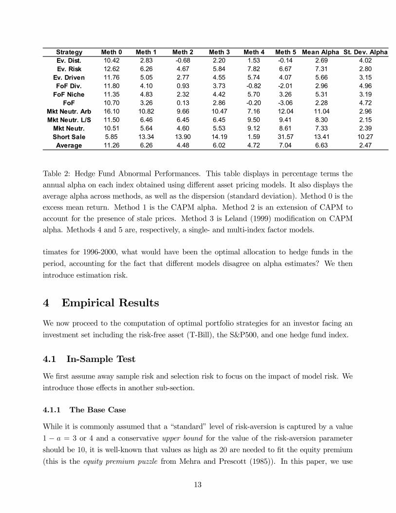
In table 2, we present the alpha on each index obtained using the various afore-mentioned
models, as well as the mean and standard deviation of these alphas. The latter quantity can be
regarded as a real-world empirical estimate of uncertainty about alpha driven by model risk.
As can be seen from these numbers, model risk induces a significant amount of uncertainty
15The CSFB/Tremont indices cover nine strategies (convertible arbitrage, dedicated short bias, emergingmarkets, equity market neutral, event driven, fixed-income arbitrage, global macro, long-short equity, managedfutures), and is based on 340 funds representing $100 billion in invested capital, selected from a database, theTASS database, which tracks over 2,600 funds. Amenc and Martellini (2002b) have introduced a set of “purestyle indices” and tested their superior power in the context of style analysis. We do not, however, use thesepure style indices because data is not available before 1998.16The reader should be cautioned that this average fund can not be regarded as an equally-weighted index
of all funds in the data base. For example the 6.63% volatility of the so-called average fund is the average ofall funds volatility, and not the volatility of a fund posting performance the equally-weighted average of theperformance on each fund.
Table 2: Hedge Fund Abnormal Performances. This table displays in percentage terms the
annual alpha on each index obtained using different asset pricing models. It also displays the
average alpha across methods, as well as the dispersion (standard deviation). Method 0 is the
excess mean return. Method 1 is the CAPM alpha. Method 2 is an extension of CAPM to
account for the presence of stale prices. Method 3 is Leland (1999) modification on CAPM
alpha. Methods 4 and 5 are, respectively, a single- and multi-index factor models.
timates for 1996-2000, what would have been the optimal allocation to hedge funds in the
period, accounting for the fact that different models disagree on alpha estimates? We then
introduce estimation risk.
4 Empirical Results
We now proceed to the computation of optimal portfolio strategies for an investor facing an
investment set including the risk-free asset (T-Bill), the S&P500, and one hedge fund index.
4.1 In-Sample Test
We first assume away sample risk and selection risk to focus on the impact of model risk. We
introduce those effects in another sub-section.
4.1.1 The Base Case
While it is commonly assumed that a “standard” level of risk-aversion is captured by a value
1 − a = 3 or 4 and a conservative upper bound for the value of the risk-aversion parameter
should be 10, it is well-known that values as high as 20 are needed to fit the equity premium
(this is the equity premium puzzle from Mehra and Prescott (1985)). In this paper, we use
13
a = −15 as a base case value; this is consistent with a³1− mp−r
σ2P (1−a), mp−rσ2P (1−a)
´= (68.2%, 31.8%)
Merton (1973) allocation to the risk-free versus risky asset. We also perform some comparative
static analysis on the risk aversion a parameter. We use the mean T-Bill rate on the period
(5.06%) as an estimate of the risk-free rate r. The average return on the S&P500 on the
period is 18.23%, and will be regarded as the value for mp, which we assume identical to
the true population value for the moment (δP = 0). The annual volatility on the S&P500
volatility is estimated at σP = 16.08% from monthly data over the period 1996-2000. Finally,
we arbitrarily fix the time-horizon at a T = 5 value.17
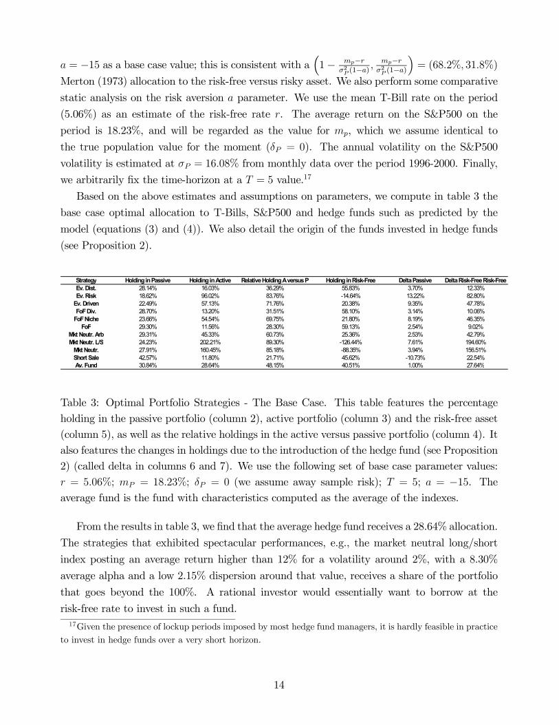
Based on the above estimates and assumptions on parameters, we compute in table 3 the
base case optimal allocation to T-Bills, S&P500 and hedge funds such as predicted by the
model (equations (3) and (4)). We also detail the origin of the funds invested in hedge funds
(see Proposition 2).
Strategy Holding in Passive Holding in Active Relative Holding A versus P Holding in Risk-Free Delta Passive Delta Risk-Free Risk-FreeEv. Dist. 28.14% 16.03% 36.29% 55.83% 3.70% 12.33%Ev. Risk 18.62% 96.02% 83.76% -14.64% 13.22% 82.80%
Table 3: Optimal Portfolio Strategies - The Base Case. This table features the percentage
holding in the passive portfolio (column 2), active portfolio (column 3) and the risk-free asset
(column 5), as well as the relative holdings in the active versus passive portfolio (column 4). It
also features the changes in holdings due to the introduction of the hedge fund (see Proposition
2) (called delta in columns 6 and 7). We use the following set of base case parameter values:
r = 5.06%; mP = 18.23%; δP = 0 (we assume away sample risk); T = 5; a = −15. Theaverage fund is the fund with characteristics computed as the average of the indexes.
From the results in table 3, we find that the average hedge fund receives a 28.64% allocation.
The strategies that exhibited spectacular performances, e.g., the market neutral long/short
index posting an average return higher than 12% for a volatility around 2%, with a 8.30%
average alpha and a low 2.15% dispersion around that value, receives a share of the portfolio
that goes beyond the 100%. A rational investor would essentially want to borrow at the
risk-free rate to invest in such a fund.17Given the presence of lockup periods imposed by most hedge fund managers, it is hardly feasible in practice
to invest in hedge funds over a very short horizon.
14
More generally, our analysis provides formal backing to the widely spread notion that
investors should use hedge funds as substitutes for some portion of their risk-free asset holdings
(see Proposition 2). The origin of the 28.64% now allocated to the average active portfolio are
27.64% from the risk-free asset versus 1.00% from the passive portfolio (remember that the
beta of the average fund is 0.03).
4.1.2 Impact of Biases
We now penalize the estimated expected return on all hedge funds by 4.5%, a reasonable
estimate of effect of survivorship, selection and instant history biases, and obtain the following
results (under the same base case parameter values).18
Strategy Holding in Passive Holding in Active Relative Holding A versus P Holding in Risk-Free Delta Passive Delta Risk-Free Risk-FreeEv. Dist. 34.32% -10.75% -45.60% 76.43% -2.48% -8.27%Ev. Risk 26.76% 36.94% 57.99% 36.31% 5.09% 31.85%
Table 4: Optimal Portfolio Strategies - The Impact of Biases. This table features the percent-
age holding in the passive portfolio (column 2), active portfolio (column 3) and the risk-free
asset (column 5), as well as the relative holdings in the active versus passive portfolio (column
4). It also features the changes in holdings due to the introduction of the hedge fund (see
Proposition 2) (called delta in columns 6 and 7). We use the following set of base case para-
meter values: r = 5.06%; mP = 18.23%; δP = (7.19%)2 = .52%; T = 5; a = −15. We penalize
the estimated expected return on a hedge fund by 4.5%, a reasonable estimate of effect of
survivorship, selection and instant history biases.
From the results in table 4, we find that the willingness of investors to hold hedge funds
has severely declined as a result of expected returns being deflated by 4.5%. The holdings in
the average hedge fund have decreased from 28.64% down to 9.20%, which is consistent with
what most investors allocate to hedge funds.19 Moreover, the optimal holdings in any hedge
fund exhibiting an average alpha lower than 4.5% are now negative, as can be expected from
equation (3).
18In principle, the presence of biases not only affect expected return on hedge funds, but also beta andvolatility estimate (for more details on this, see Amenc, Martellini and Vaissie (2002)).19From informal conversations with various people in industry, it actually appears that most asset allocators
would heuristically argue for a 10 to 20% allocation to hedge funds as a reasonable number.
15
4.1.3 Impact of Time-Horizon
We have argued that, for non trivial uncertainty around the alpha of the active portfolio,
an increase in time horizon leads to an increase in the holdings in the passive portfolio, and
therefore a decrease in the relative holdings in the active portfolio. The intuition is that time
allows for uncertainty around alpha to unfold and hurt the risk-averse investor. On the other
hand, when there is no uncertainty around alpha (see equation (3)), the solution is time-horizon
independent.
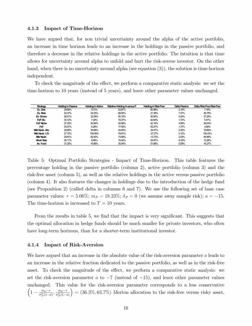
To check the magnitude of the effect, we perform a comparative static analysis: we set the
time-horizon to 10 years (instead of 5 years), and leave other parameter values unchanged.
Strategy Holding in Passive Holding in Active Relative Holding A versus P Holding in Risk-Free Delta Passive Delta Risk-Free Risk-FreeEv. Dist. 29.69% 9.31% 23.87% 60.99% 2.15% 7.16%Ev. Risk 24.37% 54.25% 69.00% 21.38% 7.47% 46.78%
Table 5: Optimal Portfolio Strategies - Impact of Time-Horizon. This table features the
percentage holding in the passive portfolio (column 2), active portfolio (column 3) and the
risk-free asset (column 5), as well as the relative holdings in the active versus passive portfolio
(column 4). It also features the changes in holdings due to the introduction of the hedge fund
(see Proposition 2) (called delta in columns 6 and 7). We use the following set of base case
parameter values: r = 5.06%; mP = 18.23%; δP = 0 (we assume away sample risk); a = −15.The time-horizon is increased to T = 10 years.
From the results in table 5, we find that the impact is very significant. This suggests that
the optimal allocation in hedge funds should be much smaller for private investors, who often
have long-term horizons, than for a shorter-term institutional investor.
4.1.4 Impact of Risk-Aversion
We have argued that an increase in the absolute value of the risk-aversion parameter a leads to
an increase in the relative fraction dedicated to the passive portfolio, as well as in the risk-free
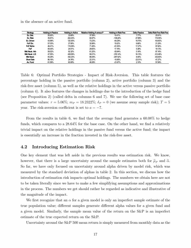
asset. To check the magnitude of the effect, we perform a comparative static analysis: we
set the risk-aversion parameter a to −7 (instead of −15), and leave other parameter valuesunchanged. This value for the risk-aversion parameter corresponds to a less conservative³1− mp−r
σ2P (1−a), mp−rσ2P (1−a)
´= (36.3%, 63.7%) Merton allocation to the risk-free versus risky asset,
16
in the absence of an active fund.
Strategy Holding in Passive Holding in Active Relative Holding A versus P Holding in Risk-Free Delta Passive Delta Risk-Free Risk-FreeEv. Dist. 55.92% 33.68% 37.59% 10.41% 7.77% 25.91%Ev. Risk 35.81% 202.43% 84.97% -138.24% 27.88% 174.55%
Table 6: Optimal Portfolio Strategies - Impact of Risk-Aversion. This table features the
percentage holding in the passive portfolio (column 2), active portfolio (column 3) and the
risk-free asset (column 5), as well as the relative holdings in the active versus passive portfolio
(column 4). It also features the changes in holdings due to the introduction of the hedge fund
(see Proposition 2) (called delta in columns 6 and 7). We use the following set of base case
parameter values: r = 5.06%; mP = 18.2322%; δP = 0 (we assume away sample risk); T = 5
year. The risk-aversion coefficient is set to a = −7.
From the results in table 6, we find that the average fund generates a 60.08% to hedge
funds, which compares to a 28.64% for the base case. On the other hand, we find a relatively
trivial impact on the relative holdings in the passive fund versus the active fund; the impact
is essentially an increase in the fraction invested in the risk-free asset.
4.2 Introducing Estimation Risk
One key element that was left aside in the previous results was estimation risk. We know,
however, that there is a large uncertainty around the sample estimates both for eµP and eα.So far, we have only focused on uncertainty around alpha driven by model risk, which was
measured by the standard deviation of alphas in table 2. In this section, we discuss how the
introduction of estimation risk impacts optimal holdings. The numbers we obtain here are not
to be taken literally since we have to make a few simplifying assumptions and approximations
in the process. The numbers we get should rather be regarded as indicative and illustrative of
the magnitude of the impact.
We first recognize that an α for a given model is only an imperfect sample estimate of the
true population value; different samples generate different alpha values for a given fund and
a given model. Similarly, the sample mean value of the return on the S&P is an imperfect
estimate of the true expected return on the S&P.
Uncertainty around the S&P 500 mean return is simply measured from monthly data as the
17
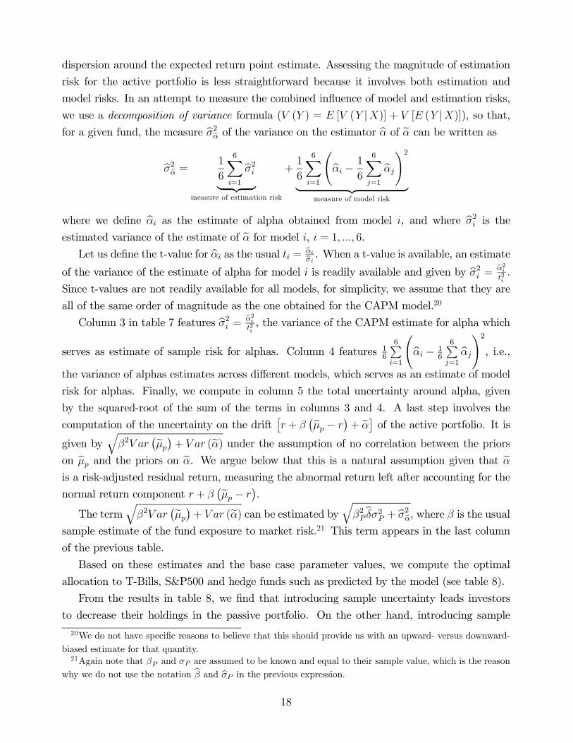
dispersion around the expected return point estimate. Assessing the magnitude of estimation
risk for the active portfolio is less straightforward because it involves both estimation and
model risks. In an attempt to measure the combined influence of model and estimation risks,
we use a decomposition of variance formula (V (Y ) = E [V (Y |X)] + V [E (Y |X)]), so that,for a given fund, the measure bσ2eα of the variance on the estimator bα of eα can be written as
bσ2eα = 1
6
6Xi=1
bσ2i| z measure of estimation risk
+1
6
6Xi=1
Ãbαi − 16
6Xj=1
bαj
!2| z
measure of model risk
where we define bαi as the estimate of alpha obtained from model i, and where bσ2i is theestimated variance of the estimate of eα for model i, i = 1, ..., 6.Let us define the t-value for bαi as the usual ti = bαibσi . When a t-value is available, an estimate
of the variance of the estimate of alpha for model i is readily available and given by bσ2i = bα2it2i.
Since t-values are not readily available for all models, for simplicity, we assume that they are
all of the same order of magnitude as the one obtained for the CAPM model.20
Column 3 in table 7 features bσ2i = bα2it2i, the variance of the CAPM estimate for alpha which
serves as estimate of sample risk for alphas. Column 4 features 16
6Pi=1
Ãbαi − 16
6Pj=1
bαj
!2, i.e.,
the variance of alphas estimates across different models, which serves as an estimate of model
risk for alphas. Finally, we compute in column 5 the total uncertainty around alpha, given
by the squared-root of the sum of the terms in columns 3 and 4. A last step involves the
computation of the uncertainty on the drift£r + β
¡eµp − r¢+ eα¤ of the active portfolio. It is
given byqβ2V ar
¡eµp¢+ V ar (eα) under the assumption of no correlation between the priorson eµp and the priors on eα. We argue below that this is a natural assumption given that eαis a risk-adjusted residual return, measuring the abnormal return left after accounting for the
normal return component r + β¡eµp − r
¢.
The termqβ2V ar
¡eµp¢+ V ar (eα) can be estimated byqβ2Pbδσ2P + bσ2eα, where β is the usual
sample estimate of the fund exposure to market risk.21 This term appears in the last column
of the previous table.
Based on these estimates and the base case parameter values, we compute the optimal
allocation to T-Bills, S&P500 and hedge funds such as predicted by the model (see table 8).
From the results in table 8, we find that introducing sample uncertainty leads investors
to decrease their holdings in the passive portfolio. On the other hand, introducing sample
20We do not have specific reasons to believe that this should provide us with an upward- versus downward-biased estimate for that quantity.21Again note that βP and σP are assumed to be known and equal to their sample value, which is the reason
why we do not use the notation bβ and bσP in the previous expression.18
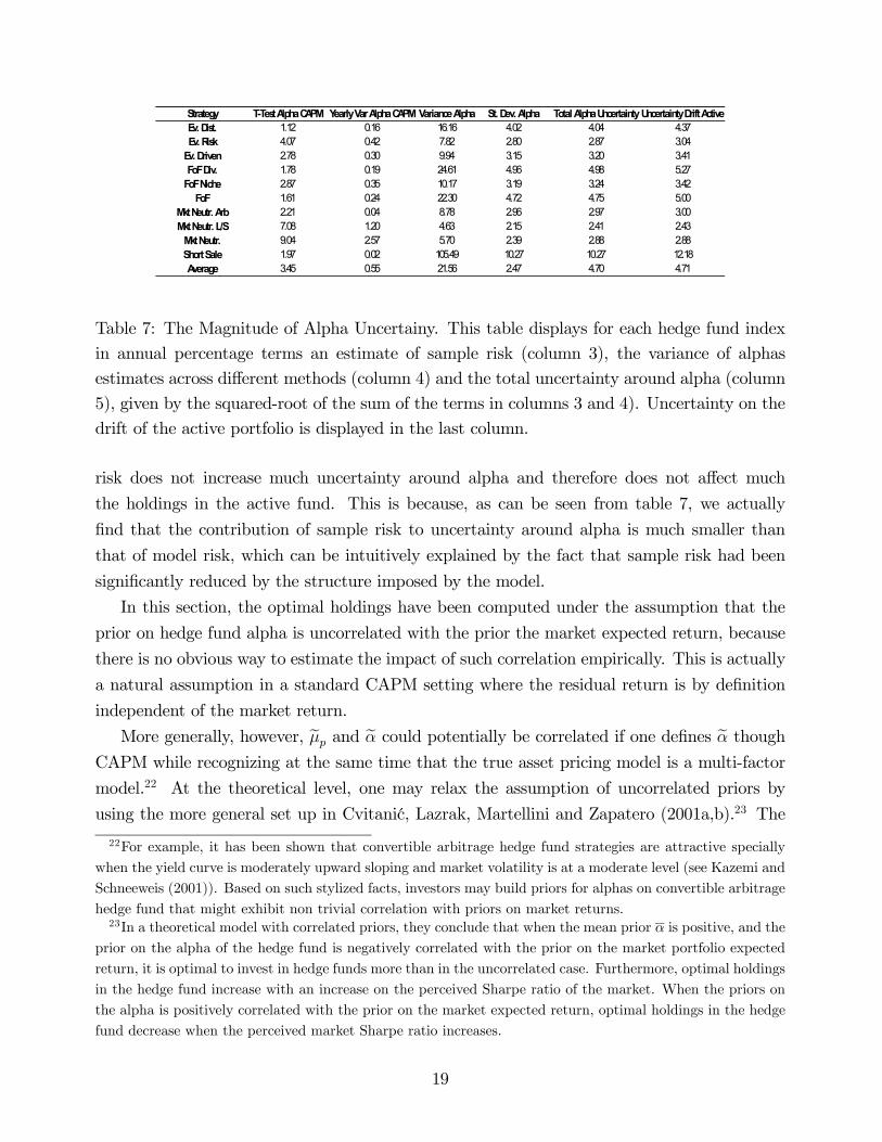
Table 7: The Magnitude of Alpha Uncertainy. This table displays for each hedge fund index
in annual percentage terms an estimate of sample risk (column 3), the variance of alphas
estimates across different methods (column 4) and the total uncertainty around alpha (column
5), given by the squared-root of the sum of the terms in columns 3 and 4). Uncertainty on the
drift of the active portfolio is displayed in the last column.
risk does not increase much uncertainty around alpha and therefore does not affect much
the holdings in the active fund. This is because, as can be seen from table 7, we actually
find that the contribution of sample risk to uncertainty around alpha is much smaller than
that of model risk, which can be intuitively explained by the fact that sample risk had been
significantly reduced by the structure imposed by the model.
In this section, the optimal holdings have been computed under the assumption that the
prior on hedge fund alpha is uncorrelated with the prior the market expected return, because
there is no obvious way to estimate the impact of such correlation empirically. This is actually
a natural assumption in a standard CAPM setting where the residual return is by definition
independent of the market return.
More generally, however, eµp and eα could potentially be correlated if one defines eα thoughCAPM while recognizing at the same time that the true asset pricing model is a multi-factor
model.22 At the theoretical level, one may relax the assumption of uncorrelated priors by
using the more general set up in Cvitanic, Lazrak, Martellini and Zapatero (2001a,b).23 The
22For example, it has been shown that convertible arbitrage hedge fund strategies are attractive speciallywhen the yield curve is moderately upward sloping and market volatility is at a moderate level (see Kazemi andSchneeweis (2001)). Based on such stylized facts, investors may build priors for alphas on convertible arbitragehedge fund that might exhibit non trivial correlation with priors on market returns.23In a theoretical model with correlated priors, they conclude that when the mean prior α is positive, and the
prior on the alpha of the hedge fund is negatively correlated with the prior on the market portfolio expectedreturn, it is optimal to invest in hedge funds more than in the uncorrelated case. Furthermore, optimal holdingsin the hedge fund increase with an increase on the perceived Sharpe ratio of the market. When the priors onthe alpha is positively correlated with the prior on the market expected return, optimal holdings in the hedgefund decrease when the perceived market Sharpe ratio increases.
19
Strategy Holding in Passive Holding in Active Relative Holding A versus P Holding in Risk-Free Delta Passive Delta Risk-Free Risk-FreeEv. Dist. 23.54% 14.19% 37.60% 62.27% 3.27% 10.91%Ev. Risk 15.20% 84.36% 84.74% 0.44% 11.62% 72.74%
Table 8: Optimal Portfolio Strategies with Estimation Risk. This table features the percentage
holding in the passive portfolio (column 2), active portfolio (column 3) and the risk-free asset
(column 5), as well as the relative holdings in the active versus passive portfolio (column
4). It also features the origin of the funds invested in the active portfolio (columns 6 and
7). We use the following set of base case parameter values: r = 5.06%; mP = 18.23%;
δP = (7.19%)2 = .52%; T = 5; a = −15.
challenge remains, however, to generate meaningful empirical estimates of such correlation.
5 Conclusion
Because the returns of alternative investment strategies exhibit in general low correlation
with that of standard asset classes, it is expected that hedge funds will take on a significant
share in active allocation strategies. While in its infancy the world of alternative investment
strategies consisted of a disparate set of managers following very specific strategies, significant
attempts at structuring the industry have occurred over the last decade which now allow
active asset allocation models to apply to hedge funds as well as to traditional investment
vehicles. In particular, investable portfolios replicating broad-based hedge funds indexes are
today available with a sufficient level of liquidity.24
In this paper we apply the model developed in Cvitanic, Lazrak, Martellini and Zapatero
(2002a,b) to a database of hedge funds. Our results have important implications for investors
who consider including alternative investment vehicles in their portfolios. In particular, they
suggest that low beta hedge funds may serve as natural substitutes for a significant portion
24In particular, Zurich Capital Markets launched a series of hedge fund indexes in 2001 that consist of equally
weighted portfolios of funds that satisfy a number of qualitative criteria for institutional investment as well asa statistical classification procedure for style classification, under the supervision of an independent advisoryboard. Investable portfolios, i.e., replicating portfolios with an approximate 2.5% tracking error, are availablefor each of these 5 indexes with monthly liquidity assured by Zurich Capital Markets (see www.zcmgroup.comfor more details).
20
of an investor risk-free asset holdings. Since the model we use can be generalized in several
directions, this paper attempts to provide money managers with a tool to allocate assets among
hedge funds.
6 References
Ackermann, C., R. McEnally, and D. Ravenscraft, 1999, The performance of hedge funds: risk,
return and incentives, Journal of Finance, 54, 3, 833-874.
Agarwal, V., and N. Naik, 2000a, On taking the alternative route: risks, rewards, and
performance persistence of hedge funds, Journal of Alternative Investments, 2, 4, 6-23.
Agarwal, V., and N. Naik, 2000b, Multi-period performance persistence analysis of hedge
funds, Journal of Financial and Quantitative Analysis, 35, 327-342.
Agarwal, V., and N. Naik, 2001, Performance evaluation of hedge funds with option-based
and buy-and-hold strategies, working paper, LBS.
Amenc, N., S. Curtis, and L. Martellini, 2001, The alpha and omega of hedge fund perfor-
mance measurement, working paper, EDHEC-MISYS Risk and Asset Management Research
Center.
Amenc, N., and L. Martellini, 2002a, Portfolio optimization and hedge fund style allocation
decisions, Journal of Alternative Investments, 5, 2, 7-20.
Amenc, N., and L. Martellini, 2002b, The brave new world of hedge fund indices, working
paper, EDHEC-MISYS Risk and Asset Management Research Center.
Amenc, N., L. Martellini, and M. Vaissié, 2002, Benefits and risks of alternative investment
strategies, working paper, EDHEC-MISYS Risk and Asset Management Research Center.
Amin, G., and H. Kat, 2001, Hedge fund performance 1990-2000. Do the “money machines”
really add value?, working paper, University of Reading.
Asness, C., R. Krail, and J. Liew, 2001, Do hedge funds hedge?, working paper, AQR
Capital Management.
Baks, K., A. Metrick and J. Wachter, 2001, Should investors avoid all actively managed
funds? A study in Bayesian performance evaluation, Journal of Finance, LVI, 1, 45-85.
Bares, P.A., R. Gibson, and S. Gyger, 2001, Style consistency and survival probability in
the hedge funds’ industry, working paper, Swiss Federal Institute of Technology and University
of Zurich.
Britten-Jones, Mark, 1999, The sampling error in estimates of mean-variance efficient port-
folio weights, Journal of Finance, 54, 2.
Brown S., and W., Goetzmann, 1997, Mutual fund styles, Journal of Financial Economics,
43, 373-399.
21
Brown S.. and W., Goetzmann, 2001, Hedge funds with style, working paper, Yale Uni-
versity.
Brown, S., W. Goetzmann, and R. Ibbotson, 1999, Offshore hedge funds: survival & per-
formance 1989-95, Journal of Business, 72, 91-117.
Cvitanic, J., A. Lazrak, L. Martellini, and F. Zapatero, 2002a, A note on portfolio selection
with partial information: power utility and Gaussian prior, working paper, USC.
Cvitanic, J., A. Lazrak, L. Martellini, and F. Zapatero, 2002b, Revisiting Treynor and
Black (1973): an intertemporal model of active management, working paper, USC.
Dimson, E., 1979, Risk measurement when shares are subject to infrequent trading, Journal
of Financial Economics, 7.
Edwards, F., and J. Liew, 1999, Hedge funds and managed futures as asset classes, Journal
of Derivatives, 45-64.
Edwards, F., and M. Caglayan, 2001, Hedge fund performance and manager skill, Journal
of Futures Markets, 21, 11, 1003-1028, .
Fung, W., and D. Hsieh, 1997a, Empirical characteristics of dynamic trading strategies,
Review of Financial Studies, 10, 275-302.
Fung, W., and D. A. Hsieh, 1997b, Survivorship bias and investment style in the returns
of CTAs, Journal of Portfolio Management, 24, 1, 30-41.
Fung, W., and D. A. Hsieh, 2000, Performance characteristics of hedge funds and CTA
funds: natural versus spurious biases, Journal of Financial and Quantitative Analysis, 35, 3,
291-307.
Fung, W., and D. A. Hsieh, 2001a, Benchmark of hedge fund performance, information
content and measurement biases, forthcoming, Financial Analysts Journal.
Fung, W., and D. A. Hsieh, 2001b, Asset-based hedge-fund styles and portfolio diversifica-
tion, working paper, Fuqua School of Business, Duke University.
Fung, W., and D. Hsieh, 2001c, The risks in hedge fund strategies: theory and evidence
from trend followers, Review of Financial Studies, 14, 313-341.
Kazemi, H., and T. Schneeweis, 2001, A comparison of hedge fund returns under different
economic conditions, working paper, CISDM, University of Armhest.
Leland, H., 1999, Beyond mean-variance: risk and performance measures for portfolios
with nonsymetric distributions, working paper, Haas School of Business, U.C. Berkeley.
Liang, B., 2000, Hedge funds: the living and the dead, Journal of Financial and Quantita-
Lhabitant, F., 2001, Hedge funds investing: a quantitative look inside the black box, work-
ing paper, Union Bancaire Privée.
22
Mehra, R., and E. Prescott, 1985, Equity premium: a puzzle, Journal of Monetary Eco-
nomics, 15, 145-161.
Merton, R. C., 1973, An intertemporal capital asset pricing model, Econometrica, 41, 867-
888.
Park J., S., Brown, and W. Goetzmann, 1999, Performance benchmarks and survivorship
bias for hedge funds and commodity trading advisors, Hedge Fund News, August 1999.
Schneeweis, T., and R. Spurgin, 1999, Multi-factor models in managed futures, hedge fund
and mutual fund estimation, working paper, CISDM, University of Armhest.
Schneeweis, T., and R. Spurgin, 2000, The benefits of index option-based strategies for
institutional portfolios, working paper, CISDM, University of Armhest.
Schneeweis, T., R. Spurgin, and D. McCarthy, 1996, Survivor bias in commodity trading
advisor performance, Journal of Alternative Investments, 1, 1-24.
Sharpe, W., 1964, Capital asset prices: a theory of market equilibrium under conditions of
risk, Journal of Finance, 19, 425-442.
Sharpe, W., 1988, Determining a fund’s effective asset mix, Investment Management Re-
view, 2, 6, 56-69.
Sharpe, W., 1992, Asset allocation: management style and performance measurement,
Journal of Portfolio Management, 18, 7-19.
Scholes, M., and J. Williams, 1977, Estimating betas from nonsynchronous data, Journal
of Financial Economics, 5.
A Appendix: Information on Hedge Fund Strategies
We present some information on the hedge fund strategies discussed in the paper. We refer
the reader to www.marhedge.com for more information about these strategies as well as about
others not covered in this paper.
• Event-Driven. Investment theme is dominated by events that are seen as special situa-tions or opportunities to capitalize from price fluctuations. Distressed Securities man-
agers focus on securities of companies in reorganization and/or bankruptcy, ranging from
senior secured debt (low-risk) to common stock (high risk). Risk Arbitrage managers
simultaneously buy stock in a company being acquired and sell stock in its acquirers. If
the takeover falls through, traders can be left with large losses.
• Market Neutral. The manager attempts to lock-out or neutralize market risk. In theory,market risk is greatly reduced but it is difficult to make a profit on a large diversified
portfolio, so stock picking is critical. Long/short: net exposure to market risk is believed
to be reduced by having equal allocations on the long and short sides of the market.
23
Convertible arbitrage: manager goes long convertible securities and short underlying eq-
uities, profiting from mispricing in the relationship of the two. Stock arbitrage: manager
buys a basket of stocks and sells short stock index futures contract, or reverse. Fixed
income arbitrage: manager buys bonds - often T-bonds, but also sovereign and corpo-
rate bonds - and goes short instruments that replicate the owned bond; manager aims
to profit from mispricing of relationship between the long and short sides.
• Short-Seller. Manager takes a position that stock prices will go down. A hedge fund
borrows stock and sells it, hoping to buy it back at a lower price. Manager shorts only
overvalued securities.
• Fund of Funds. Capital is allocated among funds, providing investors with access tomanagers with higher minimums than individual might afford. Diversified funds of funds
allocate capital to a variety of fund types. Niche funds of funds allocates capital to a