Page 1
Journal of Operation and Automation in Power Engineering
Vol. 5, No. 2, Dec. 2017, Pages: 117-130
http://joape.uma.ac.ir
Optimal Capacitor Allocation in Radial Distribution Networks for Annual Costs
Minimization Using Hybrid PSO and Sequential Power Loss Index Based
Method
J. Gholinezhad 1, R. Noroozian 2, A. Bagheri 2,*
1West Mazandaran Electric Power Distribution Company, Noshahr, Iran 2Department of Electrical Engineering, Faculty of Engineering, University of Zanjan, Zanjan, Iran
Abstract- In the most recent heuristic methods, the high potential buses for capacitor placement are initially identified
and ranked using loss sensitivity factors (LSFs) or power loss index (PLI). These factors or indices help to reduce the
search space of the optimization procedure, but they may not always indicate the appropriate placement of capacitors.
This paper proposes an efficient approach for the optimal capacitor placement in radial distribution networks with the
aim of annual costs minimization based on sequentially placement of capacitors and calculation of power loss index.
In the proposed approach, initially, the number of capacitors location is estimated using the total reactive power
demand and average range of capacitors available in the market. Then, the high potential buses can be identified using
sequential power loss index based method. This method leads to achieve the optimal or near optimal locations for the
capacitors and decrease the search space of the optimization procedure significantly. The particle Swarm Optimization
(PSO) algorithm takes the final decision for the optimum size and location of capacitors. To evaluate the efficiency of
the conducted approach, it is tested on several well-known distribution networks, and the results are compared with
those of existing methods in the literature. The comparisons verify the effectiveness of the proposed method in
producing fast and optimal solutions.
Keyword: Annual costs minimization, Capacitor allocation, Particle swarm optimizarion, Power loss reduction,
Sequential power loss index.
1. INTRODUCTION
Installation *o o o sunnto aaaaaitosso ato aaasoasiat o
loaationso ino distsibntiono n twoskso imasov so tu o d so
voltag o aso il o viao aow so aatoso aoss ation.o Tu o
aaaaaitosso d as as o tu o d mando anss nt,o syst mo loss s,o
andovoltag odsoa,ol adingotoovoltag oaso il oimasov m nto
[1].o Nnm sonso m tuodso oso solvingo oatimalo aaaaaitoso
alaa m ntoasobl mowituoaovi wo toominimiz o tu oaow so
loss souav ob nosngg st doinotu olit satns obas doonobotuo
tsaditionalo matu matiaalo m tuodso ando mos o s a nto
u nsistiao o aaasoaau so [2]. H nsistiao aaasoaau so aano
d as as o tu o matu matiaalo aomal xity.o Alsoo tu s o
m tuodsouav osaaidos saons s.oS v salou nsistiaom tuodso
uav ob nod v loa do ino tu o lastod aad o oso tu ooatimalo
aaaaaitosoalaa m nt.o
Received: 09 Sep. 2016,
Revised: 20 Nov. 2016
Accepted: 28 Dec. 2016
Corresponding author:
E-mail: [email protected] (A. bagheri)
Digital object identifier: 10.22098/joape.2017.2760.1233
2017 University of Mohaghegh Ardabili. All rights reserved.
Ao aomas u nsiv o analysiso o o tu o s a nto u nsistiao
oatimizationot auniqn sotuatosolv otu ooatimaloaaaaaitoso
alaa m nto asobl mo iso as s nt do ino [3].o Cuoosingo tu o
wuol o bns so o o n twosko aso tu o aot ntialo (aandidat )o
loaationso oso tu o aaaaaitoso alaa m nto willo s snlto ino tu o
oatimalo solntions,o bnto tu o aomantationo tim o inas as so
signi iaantlyoinst ad,oandotu oasobabilityoo oaonv sg na o
d as as so wituo inas asingo tu o siz o o o distsibntiono
n twosk.o Ino mos o s a nto u nsistiao bas do m tuods,o tu o
uiguo aot ntialo bns so oso tu o aaaaaitoso alaa m nto as o
initiallyo id nti i do ando sank do nsingo losso s nsitivityo
aatosso [2,4-8]o oso aow so losso ind xo [6,9,10].o Ino tu s o
m tuods,o som o o o tu o n twosko bns so as o nominat do
initiallyo oso aaaaaitoso alaa m nto a t so sankingo o o bns so
bas do ono LSFo oso PLI.o Altuonguo nsingo LSFo oso PLIo
signi iaantlyol adsotootu os dnationoo os asauosaaa o osotu o
oatimizationoasoa dns ,obntotu youav ob noasov nol sso
tuano satis aatosy,o ando mayo noto alwayso obtaino tu o
aaasoasiat o alaa so o o aaaaaitoso installation,o sa aially,o
wu no tu o distsibntiono n twosko s qnis so mos o tuano on o
aaaaaitoso oso tu o s aativ o aow so aoma nsation.o Foso
xamal ,obotuoLSFoandoPLIom tuodsoas ons do ino[6]o too
Page 2
J. Gholinezhad, R. Nosoozian,oA.oBagu si:ooOatimaloCaaaaitosoAlloaationoinoRadialoDistsibntionoN twoskso os… 118
id nti yo tu o aandidat o loaationso oso tu o s aativ o
aoma nsation;o tu oobtain do s snltso al aslyo indiaat o tuato
tu o PLIo ando LSFo m tuodso bas do aaaaaitoso alaa m nto
giv so b tt so s snlts,o ando n itu so o o LSFo noso PLIo
gnasant sotu omaximnmon tosavings.oTu oantuossouigulyo
s aomm nd doaaalyingobotuoPLIoandoLSFoindiaatossotoo
g to tu o oatimalo oso n aso oatimalo oa satingo aostso ando
maximnmosavings.oInoLSFoandoPLIom tuods,otu oimaaato
o os aativ oaow soinj at dobyoaaaaaitossoisonotoaonsid s do
tooid nti yotu oloaationoo otu m.oCons qn ntly,otu obns so
as onotoasoa slyosank do osomnltial oaaaaaitosoalaa m nto
byoa s osmingotu s om tuods.oInj ationoo os aativ oaow so
byoon oaaaaaitosobankoauang sotu os aativ oaow so lowoino
distsibntiono n twosks,o ando ito mayo auang o tu o sanko o o
bns so oso alaa m nto o o tu o n xto aaaaaitos,o wuiauo uav o
b no initiallyo onndobyoLSFoosoPLIom tuods.oTuns,o tu o
aaasoasiat o loaationso o o tu o aaaaaitosso suonldo b o
id nti i dobyoaddingoaaaaaitossoandosankingoo otu obns so
s qn ntially.o
Ino tuiso aaa s,o initially,o tu o nnmb so o o aaaaaitoss’o
loaationso iso aaasoximat do nsingo totalo s aativ o aow so
d mandoandotu oav sag osang oo oaaaaaitossoavailabl oino
tu omask t.oTu n,otu ouiguoaot ntialobns soas oid nti i do
nsingo tu o s qn ntialo aow so losso ind xo bas do m tuod.o
Finally,otu oPSOoalgositumoisons dotoo indotu ooatimalosiz o
andoloaationoo oaaaaaitoss.oTu ovalidityoando ativ n sso
o otu oasoaos doaaasoaauoisot st doono34-bns,o85-bns,oando
94-bnso sadialo distsibntiono n twosks,o ando tu o s snltso as o
aomaas dowituotuos oo o xistingou nsistiaobas dom tuodso
lik oAsti iaialoB oColonyo(ABC)o[2],oPSOo[4],oG n tiao
Algositumo(GA)o[11],oCnakoooS asauoAlgositumo(CSA)o
[12],o Evolntionasyo Algositumo (EA)o [13],o T aauingo
L asningo Bas do Oatimizationo (TLBO)o [14]o ando Dis ato
S asauo Algositumo (DSA)o [15].o Tu o not wostuyo
aontsibntionso o o tu o anss nto aaa so aano b o ontlin do aso
ollows:
Psoaosingoano iai ntoaaasoaauo osooatimaloaaaaaitoso
alloaationowituotu oaimoo oannnaloaostsominimization;
D t sminingo tu o aot ntialo (aandidat )o loaationso oso
aaaaaitosso nsingo s qn ntialo alaa m nto o o aaaaaitosso
andoaalanlationoo oaow solossoind x;
UsingoaoPSOoalgositumotoooatimallyos l atoamongotu o
aot ntialobns so osotu oaaaaaitosoinstallation;
Fasto aonv sg na o ando oatimalo solntionso o o tu o
aondnat do aaasoaauo aomaas do too tu o xistingo
m tuods.
Tu o s maind soo o tuisoaaa so isoosganiz doaso ollows:o
Tu oloado lowom tuodoisosnmmasiz doinotu on xtos ation.o
S ationo3oas s ntsotu os qn ntialoPLIobas dom tuodo oso
oatimaloaaaaaitosoalloaation.oTu oobj ativ o nnationoando
PSOoalgositumoas o s sa ativ lyod sasib do ino s ationso4o
ando5.oS ationo6oasovid so tu osimnlationos snltso oso tu o
aaaliaationo o o tu o asoaos do aaasoaauo ono tus o
distsibntionon twosks.oFinally,otu olastos ationoaonalnd so
tu oaaa s.
2. LOAD FLOW METHOD
Tu otsaditionaloloado lowom tuodsons doinotsansmissiono
syst ms,osnauoasotu oGanss-S id loandoN wton-Raausono
t auniqn s,o mayo b aom o in iai nto ino tu o analysiso o o
distsibntiono syst mso dn o too tu o uiguo satioo o o R/Xo ino
distsibntionosyst ms.oTu odistsibntionoaow so lowom tuodo
sngg st do ino [16]o iso ns do ino tuiso stndyo too aalanlat o tu o
voltag oo obns soandoaow so lowoo o lin s.oTuisom tuodo
solv so tu o loado lowo asobl mo dis atlyo bas do ono
aalanlationoo otwoomatsia soobtain do somotu otoaologiaalo
auasaat sistiaso o o distsibntiono syst ms.o Foso aomal t o
osmnlationoandod sasiationoo otuisoloado lowom tuod,otu o
s ad ssoas os ss dotoo[16].o
3. SEQUENTIAL PLI BASED METHOD
3.1. Estimating the number of capacitors’ location
The proposed approach is implemented by providing an
estimate oso tu o nnmb so o o aaaaaitoss’o loaation.o Tu s o
locations can be approximated using total reactive power
demand and average range of capacitors available in the
market. This number is used to identify high potential
buses for the capacitor installation. From the practical
point of view, to avoid cases of leading power factor, and
to maintain the power factor within higher lagging
values, the injected reactive power must be limited to
75% of total reactive load demand [6]. Using this
limitation and considering 750 kVAr as the average value
of available capacitors, the approximated number of
capacitors location is calculated as Eq. (1):
1
max min
0.75 ( )
( ) 1( ) / 2
busN
d
iloc
C C
Q i
N ceilQ Q
(1)
where, the ceil() function rounds a number to the next
larger integer, busN and dQ are the number of buses
and reactive power demand, respectively; maxCQ and
minCQ are the maximum and minimum range of injected
reactive power. Equation (1) yields an approximate
number of capacitors location. The optimal number of
capacitors location may be higher or lower, which has to
be set manually by the user.
Page 3
Journal of Operation and Automation in Power Engineering, Vol. 5, No. 2, Dec. 2017 119
3.2. Identification of buses using sequential PLI
based method
To identify high potential buses, the procedure of PLI
calculation must be run locN times by sequentially
adding the capacitors to the network. In each time, after
ranking of buses by PLI, the best location is identified
and then excluded for the next time. The PLI is calculated
by the following expression [6]:
busminmax
min N,...,,i,LRLR
LR)i(LR)i(PLI 32
(2)
where, LR is the power loss reduction compared to initial
power loss due to injection of reactive power to ith bus.
Unlike PLI calculation in [10], the reactive power
injection is not equal to reactive power demand of each
bus. After intensive trials, step changes of reactive power
injection around an average value of capacitors are led to
achieve the optimal or near to optimal locations for
capacitors. The reactive power injection in each time is
calculated as follows:
1 1
0.75 ( ) 0.75 ( )
( ) ( ) *
1, 2, ...,
bus busN N
d d
i i
C
loc loc
loc
Q i Q i
Q j F jN N
j N
(3)
The first term of Eq. (3) shows the average value for
locN capacitors. ( )F j is decreased linearly according to
Eq. (4).
1
121
100
2
loc
loc
N
j/)N(*
X)j(F (4)
where, X is a percentage of tolerance around the average
value. There is a direct relation between the optimal value
of X andotu osatiooo omaximnm/av sag oo oloads’os aativ o
power. The following steps identify the buses for
capacitor placement using the sequential PLI based
method:
(a) Run the load flow and obtain initial real power loss;
(b) Do for all estimated location (for j = 1:Nloc):
(b.1) Do for all buses, except slack bus:
(b.1.1) Inject capacitive reactive power equal to (3);
(b.1.2) Run load flow and obtain the real power loss;
(b.1.3) Calculate the loss reduction (LR = initial real
power loss – real power loss);
(b.2) Calculate PLI using Eq. (2);
(b.3) Sort the values of PLI in descending order;
(b.4) Set PLI(1))jHPB( ;
(b.5) Set )j(Q))jHPB((Q))jHPB((Q Cdnew
d .
In the above steps, HPB (j) stores the high potential buses
for capacitor allocation.
4. OBJECTIVE FUNCTION AND PROBLEM
CONSTRAINTS
4.1. Objective function
The objective of capacitor allocation in distribution
networks is to minimize the annual network costs
including the installation cost, annual cost of real power
loss, and also, the operation cost. Mathematically, the
objective function of problem can be formulated as Eq.
(5), where, lossP is real power loss, cN is the number of
compensated buses where the capacitors are installed.
The constant parameters of the objective function are
listed in Table 1 [10]. Moreover, the objective function
can be matched to maximize annual net saving. Annual
net saving is obtained by subtracting the Cost after
compensation from the Cost before compensation.
Table 1. The constant parameters of the objective function
Parameter description Value
Average energy cost (Ke) $0.06/kWh
Depreciation factor (α) 20%
Purchase cost (Cp) $25/kVAr
Installation cost (Ci) $1600/location
Operating cost (Co) $300/year/location
Hours per year (T) 8760
4.2. Constraints
The objective function is subjected to the following
operational constraints:
Reactive power compensation limits as Eq. (7).
Buses voltage limit as Eq. (8).
The apparent power flow of lines as Eq. (9).
In these expressions, minV and maxV are the minimum
and maximum voltage limits, V(i) is the voltage
amplitude of ith bus, Nbus is the number of network buses,
and Nline is the number of network lines.
5. PSO ALGORITHM
PSO algorithm is used in this work to find the optimal
size and location of capacitors. PSO is a population based
stochastic optimization technique developed by Kennedy
and Eberhart [17]. This algorithm has been widely used
for optimization of various power system problems [18-
Page 4
J. Gholinezhad, R. Nosoozian,oA.oBagu si:ooOatimaloCaaaaitosoAlloaationoinoRadialoDistsibntionoN twoskso os… 120
20]. Some special advantages of the PSO over other
optimization algorithms can be outlines as below:
co
cN
icpcilosse N.C])i(Q.CN.C.[T.P.Kyear/Cost
1
(5)
co
cN
icpcilossalossbeab N.C])i(Q.CN.C.[T).PP.(KCostCostyear/Saving
1
(6)
busmaxCCminC N1,2,...,i Q)i(QQ (7)
busmaxmin N1,2,...,i V)i(VV (8)
max line( ) i 1,2,...,NS i S (9)
).(.).(.. 2211
1 t
i
t
gbest
t
ipbesti
t
i
t
i xxcrxxcrvwv (10)
11 t
i
t
i
t
i vxx (11)
Q of capacitor installed on
candidate bus #1
Q of capacitor installed on
candidate bus 2 …
Q of capacitor installed on
candidate bus #Nbus
Fig. 1. Configuration of the particles in PSO algorithm
650 500 0 850
Fig. 2. A typical particle for 4 candidate buses
The PSO algorithm is easy to implement in
MATLAB programming environment;
It has high convergence speed;
It is from the family of intelligent optimization
algorithms;
The PSO does not have genetic operators like
crossover and mutation; the particles update
themselves with the internal velocity and they also
have memory which is important to the algorithm.
PSO actually has two populations, personal bests,
and current positions; this allows greater diversity and
exploration over a single population (as it is genetic
algorithm);
The momentum effects on particle movement can
allow faster convergence (e.g. when a particle is
moving in the direction of a gradient), and more
variety/diversity in search trajectories.
In the current paper, the sequential PLI based method
reduces the search space of the problem by determining
potential (candidate) locations for the capacitors; in this
way, the problem optimization becomes easier, so that
the PSO obtains accurate results by having high
convergence speed.
The standard PSO algorithm employs a population of
particles. The particles fly through the n-dimensional
domain space. The state of each particle is represented by
its position xi = (xi1, xi2... xin) and velocity vi = (vi1, vi2...
vin). The modified velocity and position of each
individual particle can be calculated using the formulas
Eq. (10) and (11).
In Eq. (10) and (11), pbestix is the personal best
position of the particle i; tgbestx is the position of the best
particle of the swarm; 1t
iv is the velocity of ith particle at
(t+1)th iteration; tix is the current particle position; r1
and r2 are random numbers between 0 and 1; c1 is the self-
confidence (cognitive) factor, and c2 is the swarm
confidence (social) factor; w is the inertia weight which
is set to decrease linearly from about 1 to 0.6 over the
iterations.. After that the high potential (candidate) buses
for the capacitor installation are identified, the particles
of PSO algorithm are configured as the Fig. 1. In this
figure, the ith part of each particle shows the value of
installed capacitor on the corresponding bus. For
example, if the candidate buses determined by the
sequential PLI method are as 10, 18, 21, 25, a typical
particle may be as Fig. 2. According to this figure, three
capacitors with the capacities of 650, 500, and 850 kVAr
have been installed respectively on the buses 10, 18, and
25; and also, no capacitor has been installed on bus 21.
The implementation flowchart of the proposed method is
depicted in Fig. 3.
6. SIMULATION RESULTS
Page 5
Journal of Operation and Automation in Power Engineering, Vol. 5, No. 2, Dec. 2017 121
In accordance with the presented equations in the
previous section, a program is developed in MATLAB
software and the analyses have been carried out on a
computer with Intel(R) Core(TM) 2 Duo CPU @2.2
GHz, 4 GB RAM. To investigate the performance and
applicability of the proposed approach, it has been tested
on several distribution networks (15-bus, 33-bus, 34-bus,
69-bus, 85-bus, and 118-bus), and an actual 94-bus radial
distribution network. Only three distribution networks:
the 34-bus, 85-bus, and the 94-bus have been selected for
reporting in this article. To observe the effectiveness of
the proposed approach, the obtained results are compared
with the other methods. Due to the impact of loss in the
objective function calculation, all of the existing methods
Page 6
J.oGuolin zuad,oR.oNosoozian,oA.oBagu si:ooOatimaloCaaaaitosoAlloaationoinoRadialoDistsibntionoN twoskso os… 122
Start
Max iteration reached?No
Yes
Read the system input data
(bus data & line data)
Set the number of capacitors
location
Run buses identification
procedure as (2), (3), and (4)
Run load flow and evaluate the
objective function of (5)
End
Set constant values (PSO,
objective function and constraints)
Initialize the population randomly,
size of capacitors
Sort the objective function, set initial
values for personal and global bests
Update the position and the velocity
of particles using (10) and (11)
Run load flow, evaluate the objective
function, and update the best values
Print optimal
solution
Identification of
Candidate Buses
using Sequential PLI
Method
Optimizing the
Results of
Sequential PLI
Method Using PSO
Algoruthm
Fig. 3. The implementation flowchart of hybrid PSO and sequential PLI-based method
results are recalculated by the load flow technique of this
paper. The control parameters of PSO algorithm and
constraints are shown in Table 2. For producing non-
similar populations, the initial population, as reported in
Fig. 3, has been generated randomly. Off course, the
algorithm is executed several times to make sure that no
better result can be found. Also, the authors put the best
result in the initial population, and executed the program
for several times to make sure that the obtained result is
optimal. The bus voltage constraint is (1 p.u. ± 5%) for
34-bus and (1 p.u. ± 10%) for 85-bus and 94-bus test
cases, respectively. The proposed method can obtain the
optimum solution by setting the number of
high potential buses ( locN ) to 4, 5, and 3 for 34-bus,
85-bus, and 94-bus test cases, respectively. Different
results are obtained by adjusting the value of X from 0 to
90 in the proposed approach.
6.1. The 34-bus network
Page 7
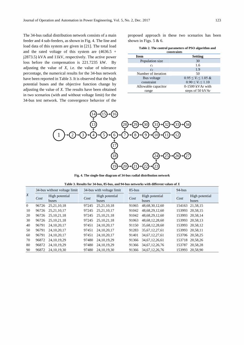
Journal of Operation and Automation in Power Engineering, Vol. 5, No. 2, Dec. 2017 123
The 34-bus radial distribution network consists of a main
feeder and 4 sub-feeders, as shown in Fig. 4. The line and
load data of this system are given in [21]. The total load
and the rated voltage of this system are (4636.5 +
j2873.5) kVA and 11kV, respectively. The active power
loss before the compensation is 221.7235 kW. By
adjusting the value of X, i.e. the value of tolerance
percentage, the numerical results for the 34-bus network
have been reported in Table 3. It is observed that the high
potential buses and the objective function change by
adjusting the value of X. The results have been obtained
in two scenarios (with and without voltage limit) for the
34-bus test network. The convergence behavior of the
proposed approach in these two scenarios has been
shown in Figs. 5 & 6.
Table 2. The control parameters of PSO algorithm and
constraints
Item Setting
Population size 30
c1 1.6
c2 1.9
Number of iteration 50
Bus voltage
constraint
0.95o≤ Vi ≤o1.05o&o
0.90o≤ Vi ≤o1.10
Allowable capacitor
range
0-1500 kVAr with
steps of 50 kVAr
2 3 41 5 6 7 8 9 10 11 12
13
14 15 16
28 29 30
17
18
19 20 21 22 23
24 25 26 27
31 32 33 34
Fig. 4. The single-line diagram of 34-bus radial distribution network
Table 3. Results for 34-bus, 85-bus, and 94-bus networks with different values of X
X
34-bus without voltage limit
34-bus with voltage limit
85-bus
94-bus
Cost High potential
buses Cost
High potential
buses Cost
High potential
buses Cost
High potential
buses
0 96726 25,21,10,18 97245 25,21,10,18 91065 48,68,30,12,60 154163 21,58,15
10 96726 25,21,10,17 97245 25,21,10,17 91042 48,68,29,12,60 153993 20,58,15
20 96726 25,10,21,18 97245 25,10,21,18 91042 48,68,29,12,60 153993 20,58,14
30 96726 25,10,21,18 97245 25,10,21,18 91063 48,68,12,28,60 153993 20,58,13
40 96791 24,10,20,17 97451 24,10,20,17 91150 35,68,12,28,60 153993 20,58,12
50 96791 24,10,20,17 97451 24,10,20,17 91283 35,67,12,27,61 153993 20,58,11
60 96791 24,10,20,17 97451 24,10,20,17 91401 34,67,12,27,61 153706 20,58,25
70 96872 24,10,19,29 97480 24,10,19,29 91366 34,67,12,26,61 153718 20,58,26
80 96872 24,10,19,29 97480 24,10,19,29 91366 34,67,12,26,76 153787 20,58,28
90 96872 24,10,19,30 97480 24,10,19,30 91366 34,67,12,26,76 153993 20,58,90
Page 8
J. Gholinezhad, R. Nosoozian,oA.oBagu si:ooOatimaloCaaaaitosoAlloaationoinoRadialoDistsibntionoN twoskso os… 124
Fig. 5. The convergence behavior of proposed method based on annual cost minimization for 34-bus network (without voltage limit)
Fig. 6. The convergence behavior of the proposed method for 34-bus network (with voltage limit)
Table 4. Optimal locations and sizes of capacitors for 34-bus system
Proposed method (X= {0,10,20,30}) Existing methods
Without
voltage limit
with
voltage limit
Discrete size Continuous size
ABC [2] EA [13] CSA [12] CSA [12] PSO [4]
Bus kVAr Bus kVAr Bus kVAr Bus kVAr Bus kVAr Bus kVAr Bus kVAr
10 600 10 600 19 950 8 1050 9 750 9 767.04 19 781
21 650 21 700 24 900 18 750 20 900 20 834.50 20 479
25 600 25 750 25 750 25 600 25 648.45 22 803
The optimal locations and sizes of capacitors obtained by
the proposed approach along with existing methods are
listed in Table 4 for the 34-bus network. The technical
and economic benefits of the proposed approach are
provided in Table 5 for comparison with the existing
methods. From Table 5, it is observed that the net yearly
savingo nsingo tu o asoaos do aaasoaauo ino “wituo voltag o
limit”osa nasiooiso$97245owuiauoisol ssotuanotuatoobtain do
by the other methods. Furthermore, the annual cost is
reduced 16.55% with 2050 kVAr installed at 3 locations
(10,o 21,o ando 25).o How v s,o ino “wituonto voltag o limit”o
scenario, the annual net saving increases to $19812 by
0.001 p.u. decrease in the minimum voltage level than
instana oo o“wituovoltag olimit”.oOn oo otu os maskabl
aspects of the proposed approach is that the
computational time for finding the optimal solution
0 10 20 30 40 509.7
9.75
9.8
9.85
9.9
9.95
10
10.05
10.1
10.15x 10
4
Iteration Number
An
nu
al
Co
sts
($)
X = 20
X = 50
X = 80
0 10 20 30 40 509.65
9.7
9.75
9.8
9.85
9.9x 10
4
Iteration Number
An
nu
al
Co
sts
($)
X = 20
X = 50
X = 80
Page 9
Journal of Operation and Automation in Power Engineering, Vol. 5, No. 2, Dec. 2017 125
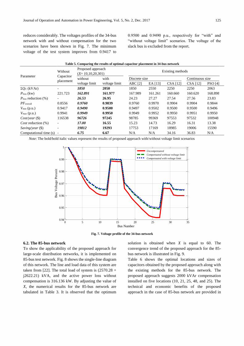
reduces considerably. The voltages profiles of the 34-bus
network with and without compensation for the two
scenarios have been shown in Fig. 7. The minimum
voltage of the test system improves from 0.9417 to
0.9500o ando 0.9490o a.n.,o s sa ativ lyo oso “witu”o ando
“wituonto voltag o limit”o sa nasios.o Tu o voltag o o o tu o
slack bus is excluded from the report.
Table 5. Comparing the results of optimal capacitor placement in 34-bus network
Parameter
Without
Capacitor
placement
Proposed approach
(X= {0,10,20,30}) Existing methods
without
voltage limit
with
voltage limit
Discrete size Continuous size
ABC [2] EA [13] CSA [12] CSA [12] PSO [4]
ΣQC (kVAr) - 1850 2050 1850 2550 2250 2250 2063
Ploss (kw) 221.723 162.891 161.977 167.989 161.261 160.660 160.620 168.898
Ploss reduction (%) - 26.53 26.95 24.23 27.27 27.54 27.56 23.83
PFoverall 0.8556 0.9760 0.9839 0.9760 0.9970 0.9904 0.9904 0.9844
Vmin (p.u.) 0.9417 0.9490 0.9500 0.9497 0.9502 0.9500 0.9500 0.9496
Vmax (p.u.) 0.9941 0.9949 0.9950 0.9949 0.9952 0.9950 0.9951 0.9950
Cost/year ($) 116538 96726 97245 98785 99369 97553 97532 100948
Cost reduction (%) - 17.00 16.55 15.23 14.73 16.29 16.31 13.38
Saving/year ($) - 19812 19293 17753 17169 18985 19006 15590
Computational time (s) - 6.75 6.67 N/A N/A 34.16 36.83 N/A
Note: The bold/bold italic values represent the results of proposed approach with/without voltage limit scenarios
Fig. 7. Voltage profile of the 34-bus network
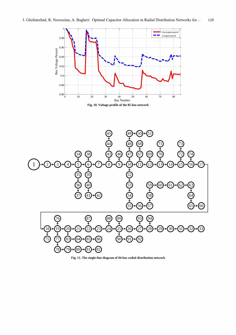
6.2. The 85-bus network
To show the applicability of the proposed approach for
large-scale distribution networks, it is implemented on
85-bus test network. Fig. 8 shows the single-line diagram
of this network. The line and load data of this system are
taken from [22]. The total load of system is (2570.28 +
j2622.21) kVA, and the active power loss without
compensation is 316.136 kW. By adjusting the value of
X, the numerical results for the 85-bus network are
tabulated in Table 3. It is observed that the optimum
solution is obtained when X is equal to 60. The
convergence trend of the proposed approach for the 85-
bus network is illustrated in Fig. 9.
Table 6 shows the optimal locations and sizes of
capacitors obtained by the proposed approach along with
the existing methods for the 85-bus network. The
proposed approach suggests 2000 kVAr compensation
installed on five locations (10, 21, 25, 48, and 25). The
technical and economic benefits of the proposed
approach in the case of 85-bus network are provided in
0 5 10 15 20 25 30 350.94
0.95
0.96
0.97
0.98
0.99
1
Bus Number
Bu
s V
olt
ag
e P
eru
nit
Uncompensated
Compensated without voltage limit
Compensated with voltage limit
Page 10
J. Gholinezhad, R. Nosoozian,oA.oBagu si:ooOatimaloCaaaaitosoAlloaationoinoRadialoDistsibntionoN twoskso os… 126
Table 7 in comparison with the existing methods. From
Table 7, it is observed that the proposed approach
achieves the minimum annual cost ($91042), and
consequently, the maximum net yearly saving ($75119).
The active power loss is reduced to 148.292 kW.
Furthermore, the overall power factor has been enhanced
from 0.7152 to 0. 9671. The voltage profile of the
network with and without compensation has been shown
in Fig. 10. The minimum voltage of this test system
improves from 0.8713 to 0.9187 p.u.
6.3. The 94-bus network
The 94-bus test case is an actual radial distribution
network with the total load of (4797 + j2323.9) kVA.
This system is illustrated in Fig. 11. The line and load
data of this system are obtained from [23]. The active
power loss of this system before the compensation is
362.8587 kW. By adjusting the value of X, the numerical
results for 94-bus networks are presented in Table 3.
Similar to 34-bus and 85-bus networks, the high potential
buses and the objective function for the 94-bus network
change by variation of X. The proposed approach
achieves the minimum cost when X equals to 60. The
convergence curve of this case is presented in Fig. 12.
Table 8 shows the optimal locations and sizes of
capacitors obtained by the proposed approach along with
the ABC based method for the 94-bus network. The
proposed approach suggests 3 locations (20, 25, and 58)
with the total reactive power of 1800 kVAr. The technical
and economic benefits of the proposed approach are
provided in Table 9 along with the results of existing
method in case 94-bus network. From Table 9, it is
observed that the proposed approach leads to 19.41%
reduction in the annual cost. The active power loss is
reduced to 271.777 kW.
2 3 41 5 6 7 8 9 10 11 12 13 14 15
24
27
25
26
29
28
30 31 32 33 34 35 36
37
38
39
4042 41
43
444547 46
48
49
50
51
53 52
54 55 56
57
5861 60
63
64
80
81
82
83 84
8578
66 65
77
67 68 69 70 71
79
59
72
73
74
75 76
16 17
20
18
19
21 22
23
62
Fig. 8. The single-line diagram of 85-bus radial distribution network
Table 6. Optimal locations and sizes of capacitors for 85-bus network
Proposed approach Existing methods
Page 11
Journal of Operation and Automation in Power Engineering, Vol. 5, No. 2, Dec. 2017 127
(X= {10,20}) Discrete size Continuous size
TLBO [14] DSA [15] CSA [12] PSO [4] GA [11] CSA [12]
Bus kVAr Bus kVAr Bus kVAr Bus kVAr Bus kVAr Bus kVAr Bus kVAr
12 400 4 300 6 150 18 150 7 324 26 48.437 8 367
29 450 7 150 8 150 27 150 8 796 28 214.06 68 356
48 400 9 300 14 150 29 300 27 901 37 103.12 32 220
60 400 21 150 17 150 42 150 58 453 38 120.31 63 313
68 350 26 150 20 150 48 300 39 178.12 12 337
30 0 26 150 60 450 51 100 44 175
31 300 30 150 69 300 54 212.5 48 347
45 150 36 450 80 450 55 101.56 21 134
49 150 57 150 59 4.687
55 150 61 150 60 157.81
61 300 66 150 61 112.5
68 300 69 300 62 104.68
83 150 80 150 66 9.375
85 150 69 100
72 67.18
74 112.5
76 71.87
80 356.25
82 31.25
Fig. 9. Convergence trend of the proposed method for 85-bus network
0 10 20 30 40 509.1
9.2
9.3
9.4
9.5
9.6
9.7
9.8x 10
4
Iteration Number
An
nu
al
Co
sts
($)
X = 0
X = 10
X = 30
X = 40
Page 12
J. Gholinezhad, R. Nosoozian,oA.oBagu si:ooOatimaloCaaaaitosoAlloaationoinoRadialoDistsibntionoN twoskso os… 128
Fig. 10. Voltage profile of the 85-bus network
2 3 41 5 6 7 8 9 10 11 12
43
44
45
39
40
41 42
56 57
58
60 61 62
49 50 51
13 14 15 16 17
18 19 20 21 22 23 24 25 26 27 28 29 30 31 32 33
35
36
37
34 38 46 47
48
52
53
54
55
59 63
64
65 66
67
68
69 70
71
72
73
74
76
75
78 79 80 81 82
77 83 84 85 86
87 88 89
90 91 92
93 94
Fig. 11. The single-line diagram of 94-bus radial distribution network
0 10 20 30 40 50 60 70 800.86
0.88
0.9
0.92
0.94
0.96
0.98
1
Bus Number
Bu
s V
olt
ag
e P
eru
nit
Uncompensated
Compensated
Page 13
Journal of Operation and Automation in Power Engineering, Vol. 5, No. 2, Dec. 2017 129
Fig. 12. The convergence trend of the proposed method based on annual costs for 94-bus network
Fig. 13. Voltage profile of the 94-bus network
Table 7. Comparing the results of optimal capacitor placement in 85-bus system
Parameter
Without
Capacitor
placement
Proposed approach
(X= {10,20})
Existing methods
Discrete size Continuous size
TLBO [14] DSA [15] CSA [12] PSO [4] GA [11] CSA [12]
ΣQC (kVAr) - 2000 2700 2550 2250 2473 2206.25 2250
Ploss (kw) 316.136 148.292 143.191 145.863 146.094 163.545 146.247 145.221
Ploss reduction (%) - 53.09 54.71 53.86 53.79 48.27 53.74 54.06
PFoverall 0.7152 0.9671 0.9999 0.9934 0.9858 0.9959 0.9830 0.9857
Vmin (p.u.) 0.8713 0.9187 0.9242 0.9179 0.9201 0.9156 0.9246 0.9216
Vmax (p.u.) 0.9957 0.9971 0.9976 0.9974 0.9973 0.9974 0.9973 0.9973
Cost/year ($) 166161 91042 96821 97475 92997 100804 99679 92538
1 11 21 31 411.536
1.538
1.54
1.542
1.544
1.546
1.548
1.55
1.552x 10
5
Iteration Number
An
nu
al
Co
sts
($)
X = 0
X = 30
X = 60
X = 70
0 10 20 30 40 50 60 70 80 900.84
0.86
0.88
0.9
0.92
0.94
0.96
0.98
1
1.02
Bus Number
Bu
s V
olt
ag
e P
eru
nit
Uncompensated
Compensated
Page 14
J. Gholinezhad, R. Nosoozian,oA.oBagu si:ooOatimaloCaaaaitosoAlloaationoinoRadialoDistsibntionoN twoskso os… 130
Cost reduction (%) - 45.21 41.73 41.34 44.03 39.33 40.01 44.31
Saving/year ($) - 75119 69340 68686 73164 65357 66482 73623
Computational time (s) - 13.25 18.38 N/A 174.86 N/A N/A 199.32
*Note: The bold values indicate the results of proposed approach
Table 8. Optimal locations and sizes of capacitors for 94-bus
system
Proposed approach (X=60) Existing method
ABC [2]
Bus kVAr Bus kVAr
20 750 18 600
25 250 21 450
58 800 54 1050
Table 9. Comparing the results of optimal capacitor placement in
94-bus system
Parameter Without
Capacitor
placement
Proposed
approach
(X=60)
Existing
method
ABC [2]
ΣQC (kVAr) - 1800 2100
Ploss (kw) 362.858 271.777 271.359
Ploss reduction (%) - 25.10 25.22
PFoverall 0.8769 0.9846 0.9931
Vmin (p.u.) 0.8485 0.9036 0.9072
Vmax (p.u.) 0.9951 0.9967 0.9970
Cost/year ($) 190718 153706 154986
Cost reduction (%) - 19.41 18.74
Saving/year ($) - 37012 35732
Computational time
(s)
- 13.54 N/A
*Note: The bold values indicate the results of proposed
approach
Moreover, the overall power factor has been enhanced
from 0.8769 to 0.9846. The voltage profile of the 94-bus
network with and without compensation has been
depicted in Fig. 13. The minimum voltage of this system
improves from 0.8485 to 0.9036 p.u.
7. CONCLUSION
In this paper, a novel and simple approach named hybrid
PSO-sequential PLI has been presented and successfully
applied to the capacitor allocation problem in radial
distribution networks. The objective function is to
minimize the annual network costs. In the proposed
approach, after estimating the number of capacitors
locations, these locations have been identified by adding
capacitors and calculating PLI (Power Loss Index)
sequentially. This approach can determine the buses for
the capacitor installation by tuning the value of tolerance
percentage (X). Finally, the optimal locations and sizes of
the capacitors have been obtained by the PSO algorithm.
The validity and effectiveness of the proposed approach
is tested on 34-bus, 85-bus, and 94-bus radial distribution
networks. The numerical results confirm that the
proposed method is capable of finding optimal solution
better than the other methods reported in the literature.
Furthermore, due to restriction of the optimization search
space to the number of estimated locations, the proposed
approach has a fast convergence toward the optimal
solutions. Implementation of the proposed approach
results in more power loss reduction, more power factor
correction, better voltage profile, and the increase in
annual network saving.
REFERENCES
[1] A.o A.o Sallam,o O.o P.o Malik,o “El atsiao distsibntiono
syst ms”,oJounoWil yoandoSons,oN woJ ss y,o2011.
[2] A. A. El-Fergany, A. Almoataz, Y. Abdelaziz,
“Caaaaitoso alaa m nt for net saving maximization
and system stability enhancement in distribution
networks using artificial bee colony-based
aaasoaau”,oElectr. Power Energy Syst., vol. 54, pp.
235-243, 2014.
[3] R.o Sisjani,o M.o Azau,o H.o Suas ,o “H nsistiao
optimization techniques to determine optimal
capacitor placement and sizing in radial distribution
n twosks:o ao aomas u nsiv o s vi w”,o Electr. Rev.,
vol. 88, no. 7a, pp. 1-7, 2012.
[4] K.o Psakasu,o M.o Sydnln,o “Pastial o swasmo
optimization based capacitor placement on radial
distribution syst ms”,o IEEE Power Eng. Soc. Gen.
Meeting, pp. 1-5, 2007.
[5] RS. Rao, SVL. Narasimham, M. Ramalingaraju,
“Oatimaloaaaaaitosoalaa m ntoinoaosadialodistsibntiono
system using plant growtuo simnlationo algositum”,o
Electr. Power Energy Syst., vol. 33, no. 5, pp. 1133-
1139, 2011.
[6] A. A. El-F sgany,o “Oatimalo aaaaaitoso alloaationso
nsingo volntionasyoalgositum”,oIET Gener. Transm.
Distrib., vol. 7, no. 6, pp. 593-601, 2013.
[7] Y.o Suniab,o M.o Kalavatui,o C.o Rajan,o “Oatimalo
capacitor placement in radial distribution system
usingogsavitationalos asauoalgositum”,oElectr. Power
Energy Syst., vol. 64, pp. 384-397, 2015.
[8] A.Y.oAbd laziz,oE.S.oAli,oS.M.oAbdoElazim,o“Flow so
pollination algorithm and loss sensitivity factors for
optimal sizing and placement of capacitors in radial
distsibntiono syst ms”,o Electr. Power Energy Syst.,
vol. 78, pp. 207-214, 2016.
[9] A. A. El-F sgany,oA.oY.oAbd laziz,o“Cnakooos asau-
based algorithm for optimal shunt capacitors
alloaationsoinodistsibntionon twosks”,oElectr. Power
Compon. Syst., vol. 41, no. 16, pp. 1567-1581, 2013.
[10] A. A. El-F sgany,o A.Y.o Abd laziz,o “Caaaaitoso
allocations in radial distribution networks using
anakooo s asauo algositum”,o IET Gener. Transm.
Distrib., vol. 8, no. 2, pp. 223-232, 2014.
Page 15
Journal of Operation and Automation in Power Engineering, Vol. 5, No. 2, Dec. 2017 131
[11] M.oSydnln,oV.oV.oK.oR ddy,o“Ind xoandoGAobas do
optimal location and sizing of distribution system
aaaaaitoss”,o IEEE power Eng. Soc. Gen. Meeting,
pp. 1-4, 2007.
[12] S. K. Injeti, V. K. Thunuguntla, M. Shareef,
“Oatimalo alloaationo o o aaaaaitoso bankso ino sadialo
distribution systems for minimization of real power
loss and maximization of network savings using bio-
insais do oatimizationo algositums”,o Electr. Power
Energy Syst., vol. 69, pp. 441-455, 2015.
[13] A.oElmaonuab,oM.oBondons,oR.oGn ddonau ,o“N wo
evolutionary technique for optimization shunt
capacitors in distributiono n twosks”,o Electr. Eng.,
vol. 62, no. 3, pp. 163-167, 2011.
[14] S.o Sn ua,o R.o Psovaso Knmas,o “Oatimalo aaaaaitoso
placement in radial distribution systems using
t aauingo l asningo bas do oatimization”,o Electr.
Power Energy Syst., vol. 54, pp. 387-398, 2014.
[15] M. R. Raju, K. V. S. R. Murthy, K. R. Avindra,
“Dis ato s asauo algositumo oso aaaaaitiv o
aoma nsationoinosadialodistsibntionosyst ms”,oElectr.
Power Energy Syst., vol. 42, no. 1, pp. 24-30, 2012.
[16] J.o H.o T ng,o “Ao dis ato aaasoaauo oso distsibntiono
system load flowo solntions”,o IEEE Trans. Power
Delivery, vol. 18, no. 3, pp. 882-887, 2003.
[17] J.o K nn dy,o R.o Eb suast,o “Pastial o swasmo
oatimization”,o Psoa. IEEE Int. Conf. Neural
Networks, pp. 1942-1948, 1995.
[18] M. Darabian, A. Jalilvand, R. Noroozian,
“Combin do ns o o o s nsitivityo analysiso ando uybsido
Wavelet-PSO-ANFIS to improve dynamic
performance of DFIG-bas do windo g n sation”,o J.
Oper. Autom. Power Eng., vol. 2, no. 1, pp. 60-73,
2007.
[19] H.o Suay gui,o A.o Guas mi,o “FACTSo d via so
allocation using a novel dedicated improved PSO for
optimal operation of power system”, J. Oper.
Autom. Power Eng., vol. 1, no. 2, pp. 124-135, 2013.
[20] E.o Baba i,o A.o Guosbani,o “Combin do aonomiao
dispatch and reliability in power system by using
PSO-SIFoalgositum”,oJ. Oper. Autom. Power Eng.,
vol. 3, no. 1, pp. 23-33, 2015.
[21] M.o Cuis,o MMA.o Salama,o S.o Jayasam,o “Caaaaitoso
placement in distribution systemusing heuristic
s asauostsat gi s”,oIET Gener. Transm. Distrib., vol.
144, no. 3, pp. 225-230, 1997.
[22] D.o Das,o D.o P.o Kotuasi,o A.o Kalam,o “Simal o ando
efficient method for load flow solution of radial
distsibntiono n twosk”,o Electr. Power Energy Syst.,
vol. 17, no. 5, pp. 335-346, 1995.
[23] D.oF.oPis s,oCH.oAntnn s,oA.G.oMastins,o“NSGA-II
with local search for a multi-objective reactive
aow so aoma nsationo asobl m”,o Electr. Power
Energy Syst., vol. 43, no. 1, pp. 313-324, 2012.