A. Ismael F. Vaz and Eugénio C. Ferreira XXIX Congreso Nacional de Estadística e Investigación Operativa, Tenerife, 15-19 May, 2006 - p. 1/31 Optimal control of fed-batch processes with particle swarm optimization A. Ismael F. Vaz Departamento de Produção e Sistemas Escola de Engenharia, Universidade do Minho [email protected]Eugénio C. Ferreira Centro de Engenharia Biológica Escola de Engenharia, Universidade do Minho [email protected]
Transcript
A. Ismael F. Vaz and Eugénio C. Ferreira XXIX Congreso Nacional de Estadística e Investigación Operativa, Tenerife, 15-19 May, 2006 - p. 1/31
Optimal control of fed-batch processes withparticle swarm optimization
A. Ismael F. VazDepartamento de Produção e Sistemas
A. Ismael F. Vaz and Eugénio C. Ferreira XXIX Congreso Nacional de Estadística e Investigación Operativa, Tenerife, 15-19 May, 2006 - p. 2/31
Contents
● The fed-batch optimal control problem
● The used approach to solve the optimal control problem
● The particle swarm paradigm
● Numerical results and conclusions
Contents❖ Contents
A. Ismael F. Vaz and Eugénio C. Ferreira XXIX Congreso Nacional de Estadística e Investigación Operativa, Tenerife, 15-19 May, 2006 - p. 2/31
Contents
● The fed-batch optimal control problem
● The used approach to solve the optimal control problem
● The particle swarm paradigm
● Numerical results and conclusions
Optimal control❖ Motivation❖ The control
problem❖ The control
problem❖ Approach❖ Nonlinear
programming(NLP)
❖ Nonlinearoptimization
A. Ismael F. Vaz and Eugénio C. Ferreira XXIX Congreso Nacional de Estadística e Investigación Operativa, Tenerife, 15-19 May, 2006 - p. 3/31
Optimal control
Optimal control❖ Motivation❖ The control
problem❖ The control
problem❖ Approach❖ Nonlinear
programming(NLP)
❖ Nonlinearoptimization
A. Ismael F. Vaz and Eugénio C. Ferreira XXIX Congreso Nacional de Estadística e Investigación Operativa, Tenerife, 15-19 May, 2006 - p. 4/31
Motivation
● A great number of valuable products are produced usingfermentation processes and thus optimizing such processesis of great economic importance.
● Fermentation modeling process involves, in general, highlynonlinear and complex differential equations.
● Often optimizing these processes results in controloptimization problems for which an analytical solution is notpossible.
Optimal control❖ Motivation❖ The control
problem❖ The control
problem❖ Approach❖ Nonlinear
programming(NLP)
❖ Nonlinearoptimization
A. Ismael F. Vaz and Eugénio C. Ferreira XXIX Congreso Nacional de Estadística e Investigación Operativa, Tenerife, 15-19 May, 2006 - p. 5/31
The control problem
● The optimal control problem is described by a set ofdifferential equations x = f(x, u, t), x(t0) = x0, t0 ≤ t ≤ tf .
● The performance index J can be generally stated as
J(tf ) = ϕ(x(tf ), tf ) +
∫ tf
t0
φ(x, u, t)dt,
where ϕ is the performance index of the state variables atfinal time tf and φ is the integrated performance index duringthe operation.
● constraints that often reflet some physical limitation of thesystem are imposed.
Optimal control❖ Motivation❖ The control
problem❖ The control
problem❖ Approach❖ Nonlinear
programming(NLP)
❖ Nonlinearoptimization
A. Ismael F. Vaz and Eugénio C. Ferreira XXIX Congreso Nacional de Estadística e Investigación Operativa, Tenerife, 15-19 May, 2006 - p. 6/31
The control problem
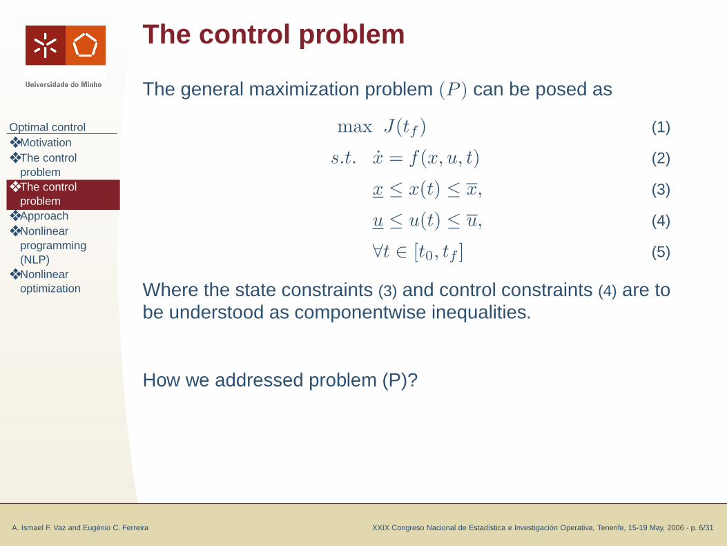
The general maximization problem (P ) can be posed as
max J(tf ) (1)
s.t. x = f(x, u, t) (2)
x ≤ x(t) ≤ x, (3)
u ≤ u(t) ≤ u, (4)
∀t ∈ [t0, tf ] (5)
Where the state constraints (3) and control constraints (4) are tobe understood as componentwise inequalities.
Optimal control❖ Motivation❖ The control
problem❖ The control
problem❖ Approach❖ Nonlinear
programming(NLP)
❖ Nonlinearoptimization
A. Ismael F. Vaz and Eugénio C. Ferreira XXIX Congreso Nacional de Estadística e Investigación Operativa, Tenerife, 15-19 May, 2006 - p. 6/31
The control problem
The general maximization problem (P ) can be posed as
max J(tf ) (1)
s.t. x = f(x, u, t) (2)
x ≤ x(t) ≤ x, (3)
u ≤ u(t) ≤ u, (4)
∀t ∈ [t0, tf ] (5)
Where the state constraints (3) and control constraints (4) are tobe understood as componentwise inequalities.
How we addressed problem (P)?
Optimal control❖ Motivation❖ The control
problem❖ The control
problem❖ Approach❖ Nonlinear
programming(NLP)
❖ Nonlinearoptimization
A. Ismael F. Vaz and Eugénio C. Ferreira XXIX Congreso Nacional de Estadística e Investigación Operativa, Tenerife, 15-19 May, 2006 - p. 7/31
Approach
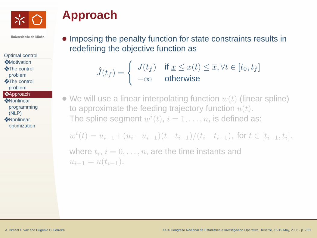
● Imposing the penalty function for state constraints results inredefining the objective function as
J(tf ) =
{
J(tf ) if x ≤ x(t) ≤ x, ∀t ∈ [t0, tf ]
−∞ otherwise
● We will use a linear interpolating function w(t) (linear spline)to approximate the feeding trajectory function u(t).The spline segment wi(t), i = 1, . . . , n, is defined as:
wi(t) = ui−1+(ui−ui−1)(t−ti−1)/(ti−ti−1), for t ∈ [ti−1, ti].
where ti, i = 0, . . . , n, are the time instants andui−1 = u(ti−1).
Optimal control❖ Motivation❖ The control
problem❖ The control
problem❖ Approach❖ Nonlinear
programming(NLP)
❖ Nonlinearoptimization
A. Ismael F. Vaz and Eugénio C. Ferreira XXIX Congreso Nacional de Estadística e Investigación Operativa, Tenerife, 15-19 May, 2006 - p. 7/31
Approach
● Imposing the penalty function for state constraints results inredefining the objective function as
J(tf ) =
{
J(tf ) if x ≤ x(t) ≤ x, ∀t ∈ [t0, tf ]
−∞ otherwise
● We will use a linear interpolating function w(t) (linear spline)to approximate the feeding trajectory function u(t).The spline segment wi(t), i = 1, . . . , n, is defined as:
wi(t) = ui−1+(ui−ui−1)(t−ti−1)/(ti−ti−1), for t ∈ [ti−1, ti].
where ti, i = 0, . . . , n, are the time instants andui−1 = u(ti−1).
Optimal control❖ Motivation❖ The control
problem❖ The control
problem❖ Approach❖ Nonlinear
programming(NLP)
❖ Nonlinearoptimization
A. Ismael F. Vaz and Eugénio C. Ferreira XXIX Congreso Nacional de Estadística e Investigación Operativa, Tenerife, 15-19 May, 2006 - p. 8/31
Nonlinear programming (NLP)
The semi-infinite programming problem is then defined as:
max J(tf )
s.t. x = f(x, w, t)
u ≤ w(t) ≤ u.
and by using the optimality conditions the SIP is redefine asthe following nonlinear programming problem.
maxu∈Rn+1
J(tf )
s.t. x = f(x, w, t)
u ≤ u(ti) ≤ u, i = 1, . . . , n.
Optimal control❖ Motivation❖ The control
problem❖ The control
problem❖ Approach❖ Nonlinear
programming(NLP)
❖ Nonlinearoptimization
A. Ismael F. Vaz and Eugénio C. Ferreira XXIX Congreso Nacional de Estadística e Investigación Operativa, Tenerife, 15-19 May, 2006 - p. 9/31
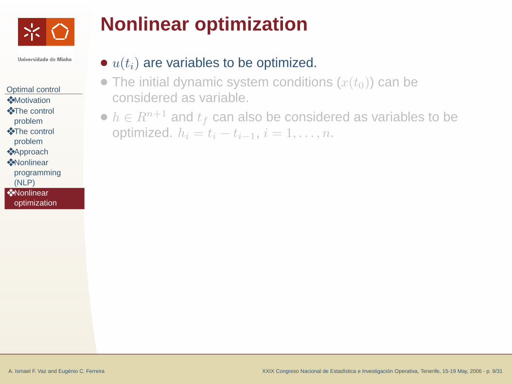
Nonlinear optimization
● u(ti) are variables to be optimized.● The initial dynamic system conditions (x(t0)) can be
considered as variable.● h ∈ Rn+1 and tf can also be considered as variables to be
optimized. hi = ti − ti−1, i = 1, . . . , n.
Optimal control❖ Motivation❖ The control
problem❖ The control
problem❖ Approach❖ Nonlinear
programming(NLP)
❖ Nonlinearoptimization
A. Ismael F. Vaz and Eugénio C. Ferreira XXIX Congreso Nacional de Estadística e Investigación Operativa, Tenerife, 15-19 May, 2006 - p. 9/31
Nonlinear optimization
● u(ti) are variables to be optimized.● The initial dynamic system conditions (x(t0)) can be
considered as variable.● h ∈ Rn+1 and tf can also be considered as variables to be
optimized. hi = ti − ti−1, i = 1, . . . , n.
w(t) is not differentiable and we will apply a derivative freealgorithm.
Global optimum is most desirable and we will apply astochastic algorithm.
The PSP❖ The Particle
Swarm Paradigm(PSP)
❖ The new travelposition andvelocity
❖ The best everparticle
❖ Features
A. Ismael F. Vaz and Eugénio C. Ferreira XXIX Congreso Nacional de Estadística e Investigación Operativa, Tenerife, 15-19 May, 2006 - p. 10/31
The PSP
The PSP❖ The Particle
Swarm Paradigm(PSP)
❖ The new travelposition andvelocity
❖ The best everparticle
❖ Features
A. Ismael F. Vaz and Eugénio C. Ferreira XXIX Congreso Nacional de Estadística e Investigación Operativa, Tenerife, 15-19 May, 2006 - p. 11/31
The Particle Swarm Paradigm (PSP)
The PSP is a population (swarm) based algorithm that mimicsthe social behavior of a set of individuals (particles).
An individual behavior is a combination of its past experience(cognition influence) and the society experience (socialinfluence).
In the optimization context a particle p, at time instant k, isrepresented by its current position (up(k)), its best everposition (yp(k)) and its travelling velocity (vp(k)).
The PSP❖ The Particle
Swarm Paradigm(PSP)
❖ The new travelposition andvelocity
❖ The best everparticle
❖ Features
A. Ismael F. Vaz and Eugénio C. Ferreira XXIX Congreso Nacional de Estadística e Investigación Operativa, Tenerife, 15-19 May, 2006 - p. 12/31
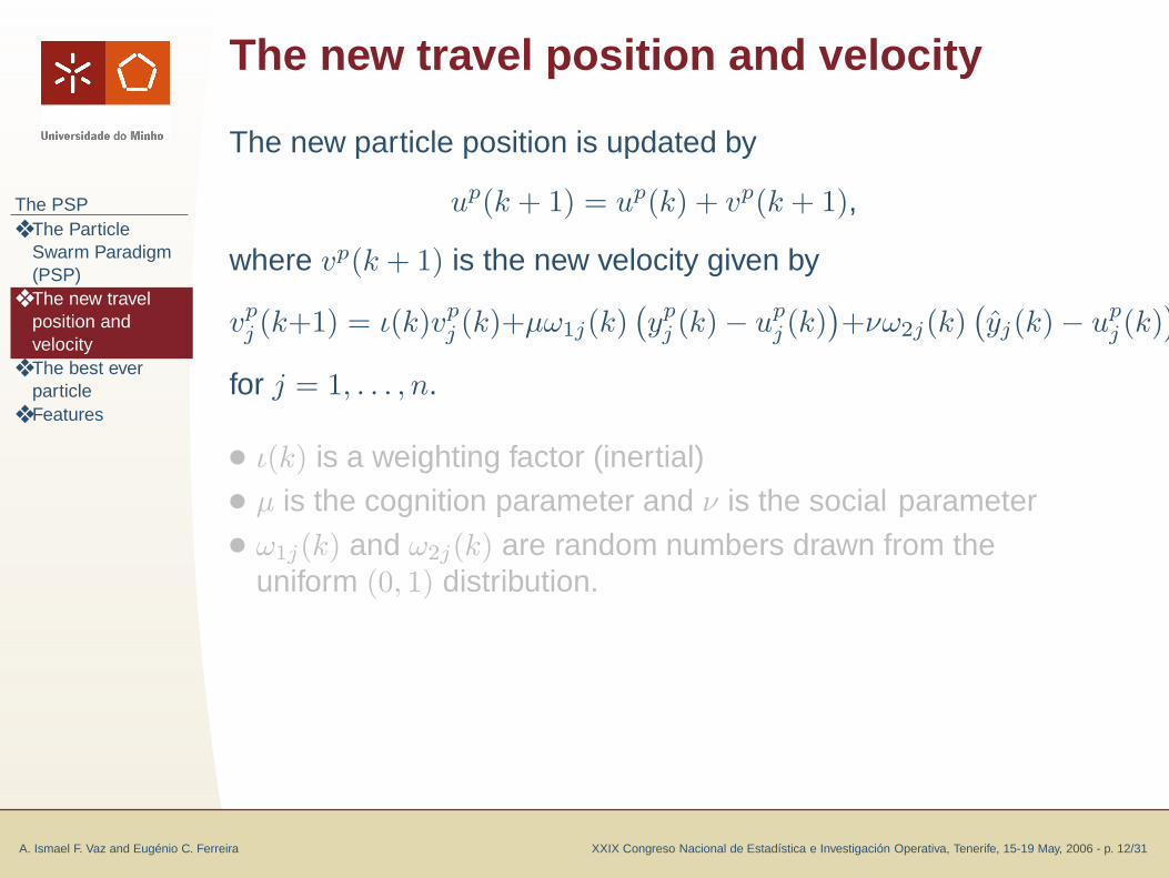
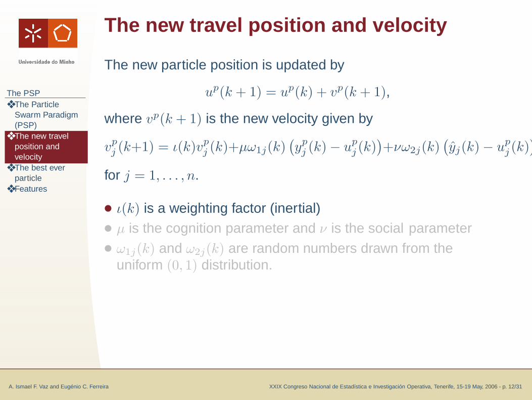
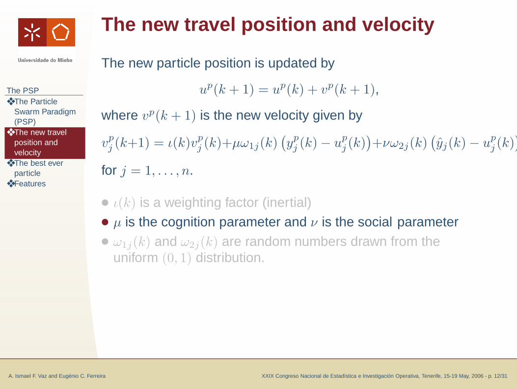
The new travel position and velocity
The new particle position is updated by
up(k + 1) = up(k) + vp(k + 1),
where vp(k + 1) is the new velocity given by
vpj (k+1) = ι(k)vp
j (k)+µω1j(k)(
ypj (k) − up
j (k))
+νω2j(k)(
yj(k) − upj (k)
)
for j = 1, . . . , n.
● ι(k) is a weighting factor (inertial)● µ is the cognition parameter and ν is the social parameter● ω1j(k) and ω2j(k) are random numbers drawn from the
uniform (0, 1) distribution.
The PSP❖ The Particle
Swarm Paradigm(PSP)
❖ The new travelposition andvelocity
❖ The best everparticle
❖ Features
A. Ismael F. Vaz and Eugénio C. Ferreira XXIX Congreso Nacional de Estadística e Investigación Operativa, Tenerife, 15-19 May, 2006 - p. 12/31
The new travel position and velocity
The new particle position is updated by
up(k + 1) = up(k) + vp(k + 1),
where vp(k + 1) is the new velocity given by
vpj (k+1) = ι(k)vp
j (k)+µω1j(k)(
ypj (k) − up
j (k))
+νω2j(k)(
yj(k) − upj (k)
)
for j = 1, . . . , n.
● ι(k) is a weighting factor (inertial)● µ is the cognition parameter and ν is the social parameter● ω1j(k) and ω2j(k) are random numbers drawn from the
uniform (0, 1) distribution.
The PSP❖ The Particle
Swarm Paradigm(PSP)
❖ The new travelposition andvelocity
❖ The best everparticle
❖ Features
A. Ismael F. Vaz and Eugénio C. Ferreira XXIX Congreso Nacional de Estadística e Investigación Operativa, Tenerife, 15-19 May, 2006 - p. 13/31
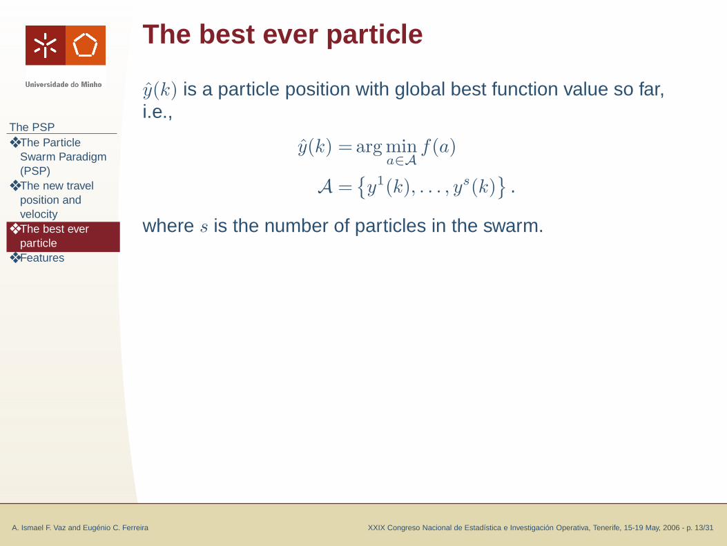
The best ever particle
y(k) is a particle position with global best function value so far,i.e.,
y(k) = arg mina∈A
f(a)
A ={
y1(k), . . . , ys(k)}
.
where s is the number of particles in the swarm.
The PSP❖ The Particle
Swarm Paradigm(PSP)
❖ The new travelposition andvelocity
❖ The best everparticle
❖ Features
A. Ismael F. Vaz and Eugénio C. Ferreira XXIX Congreso Nacional de Estadística e Investigación Operativa, Tenerife, 15-19 May, 2006 - p. 13/31
The best ever particle
y(k) is a particle position with global best function value so far,i.e.,
y(k) = arg mina∈A
f(a)
A ={
y1(k), . . . , ys(k)}
.
where s is the number of particles in the swarm.
In an algorithmic point of view we just have to keep track of theparticle with the best ever function value.
The PSP❖ The Particle
Swarm Paradigm(PSP)
❖ The new travelposition andvelocity
❖ The best everparticle
❖ Features
A. Ismael F. Vaz and Eugénio C. Ferreira XXIX Congreso Nacional de Estadística e Investigación Operativa, Tenerife, 15-19 May, 2006 - p. 14/31
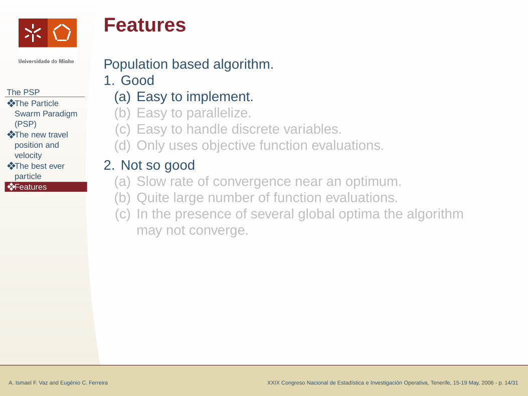
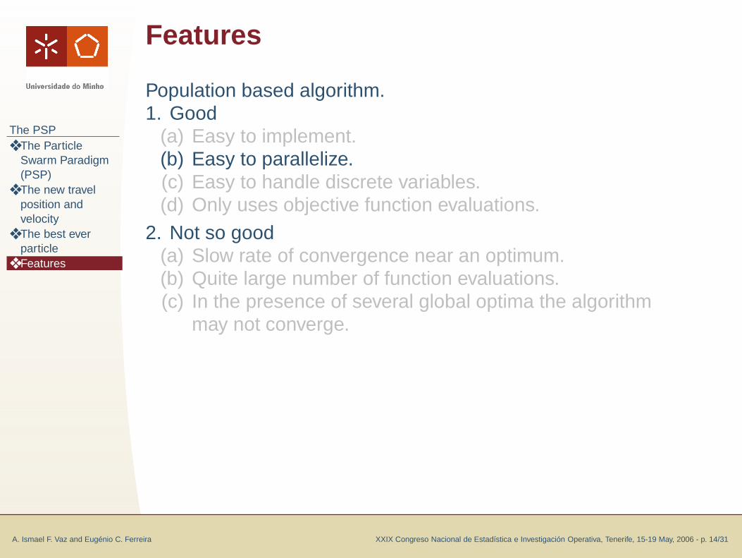
Features
Population based algorithm.1. Good
(a) Easy to implement.(b) Easy to parallelize.(c) Easy to handle discrete variables.(d) Only uses objective function evaluations.
2. Not so good(a) Slow rate of convergence near an optimum.(b) Quite large number of function evaluations.(c) In the presence of several global optima the algorithm
may not converge.
The PSP❖ The Particle
Swarm Paradigm(PSP)
❖ The new travelposition andvelocity
❖ The best everparticle
❖ Features
A. Ismael F. Vaz and Eugénio C. Ferreira XXIX Congreso Nacional de Estadística e Investigación Operativa, Tenerife, 15-19 May, 2006 - p. 14/31
Features
Population based algorithm.1. Good
(a) Easy to implement.(b) Easy to parallelize.(c) Easy to handle discrete variables.(d) Only uses objective function evaluations.
2. Not so good(a) Slow rate of convergence near an optimum.(b) Quite large number of function evaluations.(c) In the presence of several global optima the algorithm
may not converge.
Environment❖ Modeling
language - AMPL❖ Example❖ Additional
constraints❖ Some details
A. Ismael F. Vaz and Eugénio C. Ferreira XXIX Congreso Nacional de Estadística e Investigación Operativa, Tenerife, 15-19 May, 2006 - p. 15/31
Environment
Environment❖ Modeling
language - AMPL❖ Example❖ Additional
constraints❖ Some details
A. Ismael F. Vaz and Eugénio C. Ferreira XXIX Congreso Nacional de Estadística e Investigación Operativa, Tenerife, 15-19 May, 2006 - p. 16/31
Modeling language - AMPL
AMPL is a modeling language for mathematical programming.
www.ampl.com
AMPL is commercial software, but a student edition is freelyavailable.
The possibility to load an external dynamic library is exploitedin this paper in order to solve ordinary differential equations.
A short example is presented next regarding the externalfunction chemotherapy.
A. Ismael F. Vaz and Eugénio C. Ferreira XXIX Congreso Nacional de Estadística e Investigación Operativa, Tenerife, 15-19 May, 2006 - p. 17/31
Example
function chemotherapy; # external function to be called
# global search, population size of 60, maximum of 1000 iterations
solve; # solve problem
Environment❖ Modeling
language - AMPL❖ Example❖ Additional
constraints❖ Some details
A. Ismael F. Vaz and Eugénio C. Ferreira XXIX Congreso Nacional de Estadística e Investigación Operativa, Tenerife, 15-19 May, 2006 - p. 18/31
Additional constraints
Additional constraints can easily be incorporated into themodel. If, for example, a constraint in the total allowed glucoseaddition (tG) is to be imposed, the constraint
n−1∑
i=0
hi+1(ui + ui+1)/2 ≤ tG
can easily be considered in the model file by addingsubject to totalfeed:
sum {i in 0..n-1} (h[i+1]*(u[i]+u[i+1])/2)<=t_G;
and to properly define the t_G parameter.
Environment❖ Modeling
language - AMPL❖ Example❖ Additional
constraints❖ Some details
A. Ismael F. Vaz and Eugénio C. Ferreira XXIX Congreso Nacional de Estadística e Investigación Operativa, Tenerife, 15-19 May, 2006 - p. 19/31
Some details
● The ordinary differential equations are solved by calling theCVODE package where the Newton iteration with theCVDiag module was selected.
● At each call to the chemotherapy function the linear splineis computed with the provided data and the objective functionvalue is returned. The objective function expression istherefore coded in the external library.
● MLOCPSOA stands for Multi-LOCal Particle SwarmOptimization Algorithm.
● MLOCPSOA provides an interface to AMPL, allowingproblems to be easily coded and solved in this modelinglanguage.
● The NLOCPSOA allows a wide variety of algorithmparameters to be set. The used parameters are size for thepopulation size (defaults to min(6n, 1000)), maxiter for themaximum allowed iterations (defaults to 2000) and mlocalfor multi-local search (defaults to 0 – global search instead ofmulti-local search).
Numerical results❖ Parameters❖ Results❖ Results
A. Ismael F. Vaz and Eugénio C. Ferreira XXIX Congreso Nacional de Estadística e Investigación Operativa, Tenerife, 15-19 May, 2006 - p. 20/31
Numerical results
Numerical results❖ Parameters❖ Results❖ Results
A. Ismael F. Vaz and Eugénio C. Ferreira XXIX Congreso Nacional de Estadística e Investigación Operativa, Tenerife, 15-19 May, 2006 - p. 21/31
Parameters
● Numerical results were obtained for the five case studies offed-batch fermentation processes.
● The time displacements were kept fixed and the best controlfeeding trajectory was approximated by computing the knotsfunction value.
● MLOCPSOA solver used a population size of 60 and amaximum of 1000 iterations (reaching a maximum of 60000function evaluations).
● Since MLOCPSOA is a stochastic algorithm we performed10 solver runs for each problem and the best solutionsobtained are report.
A. Ismael F. Vaz and Eugénio C. Ferreira XXIX Congreso Nacional de Estadística e Investigación Operativa, Tenerife, 15-19 May, 2006 - p. 22/31
Results
MLOCPSOA Previous
Problem NT n J(tf ) tf J(tf ) tf
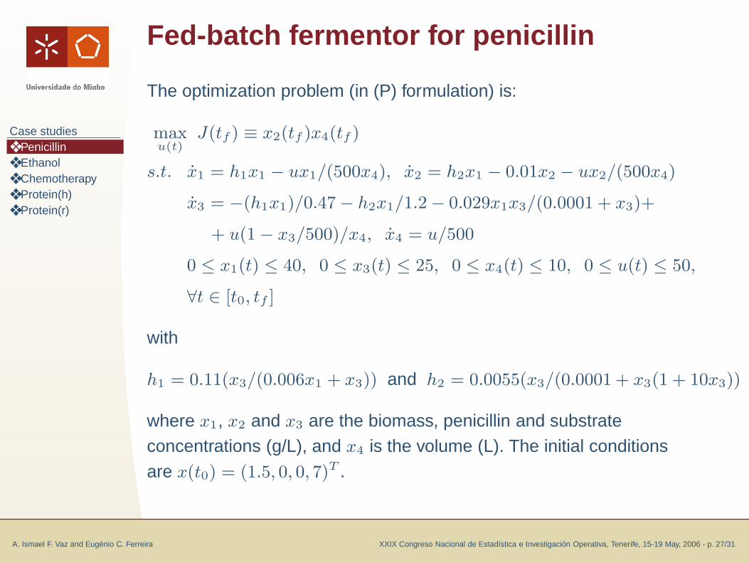
penicillin [1] 1 5 88.29 132.00 87.99 132.00
ethanol [1] 1 5 20379.50 61.20 20839.00 61.17
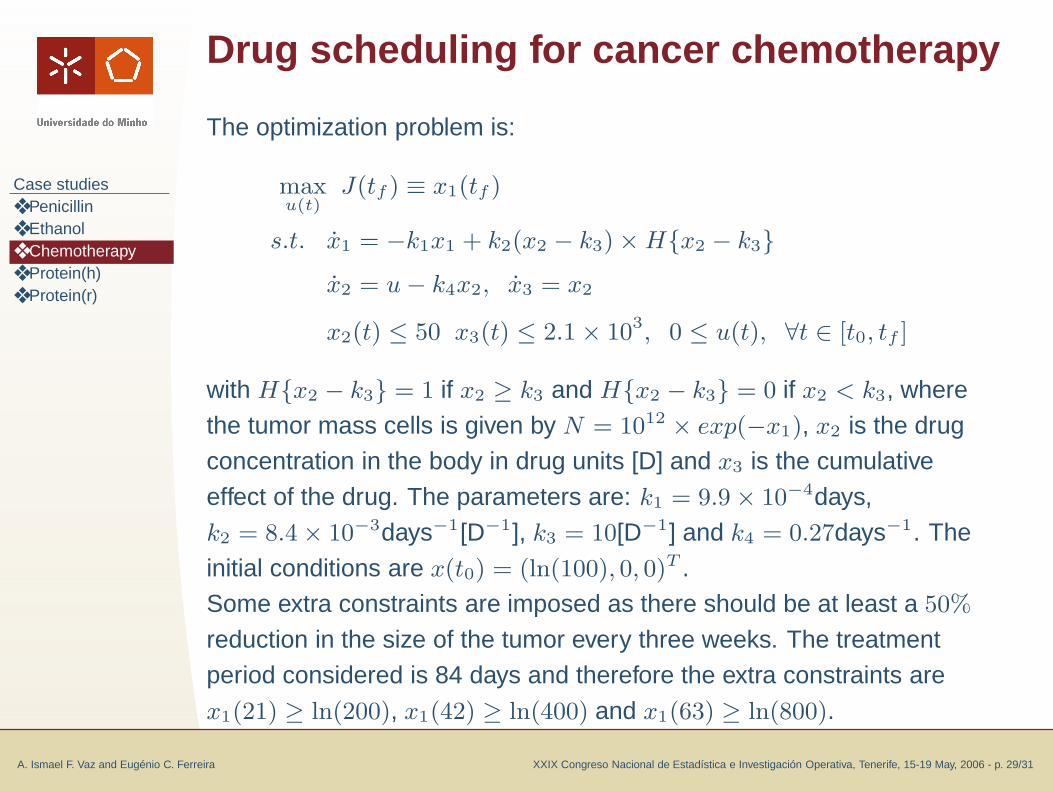
chemotherapy [1] 1 4 16.83 84.00 17.48 84.00
hprotein [2] 1 5 32.73 15.00 32.40 15.00
rprotein [3] 2 5 0.12 10.00 0.16 10.00
[1] J.R. Banga, E.Balsa-Canto, C.G. Moles, and A.A. Alonso. Dynamic optimization ofbioprocesses: Efficient and robust numerical strategies. Journal of Biotechnology,
117:407–419, 2005.[2] S. Park and W.F. Ramirez. Optimal production of secreted protein in fed-batch
reactors. AIChE Journal, 34(9):1550–1558, 1988.[3] J. Lee and W.F. Ramirez. Optimal fed-batch control of induced foreign
protein-production by recombinant bacteria. AIChE Journal, 40(5):899–907, 1994.
A. Ismael F. Vaz and Eugénio C. Ferreira XXIX Congreso Nacional de Estadística e Investigación Operativa, Tenerife, 15-19 May, 2006 - p. 23/31
Results
By allowing the spline displacements to be variable and using the objectivefunction J(tf , h) = (J(tf ))/(
∑n
i=1hi) we can easily compute the profile with the
best ratio per unit time.
Fixed time Variable time
Problem J(tf ) tf J(tf ) J(tf ) tf hmaxi
penicillin 88.29 132.00 0.92 76.16 83.20 60
ethanol 20229.50 61.20 604.20 14417.50 23.86 20
chemotherapy 16.83 84.00 0.70 8.06 11.52 25
hprotein 32.73 15.00 17.57 439.18 25 5
rprotein 0.12 10.00 2.38 59.61 25 5
With the additional constraints 0.01 ≤ hi ≤ hmaxi , i = 1, . . . , n.
Conclusions andfuture work❖ Conclusions and
future work
A. Ismael F. Vaz and Eugénio C. Ferreira XXIX Congreso Nacional de Estadística e Investigación Operativa, Tenerife, 15-19 May, 2006 - p. 24/31
Conclusions and future work
● We have shown an environment for solving optimal controlproblems
● We applied the Particle Swarm paradigm to optimal controlproblems
● The Particle Swarm paradigm proved to be a valuable tool insolving these optimal control problems
As a future research we intend to use cubic splines instead oflinear splines to approximate the trajectories.
The End❖ The End
A. Ismael F. Vaz and Eugénio C. Ferreira XXIX Congreso Nacional de Estadística e Investigación Operativa, Tenerife, 15-19 May, 2006 - p. 25/31
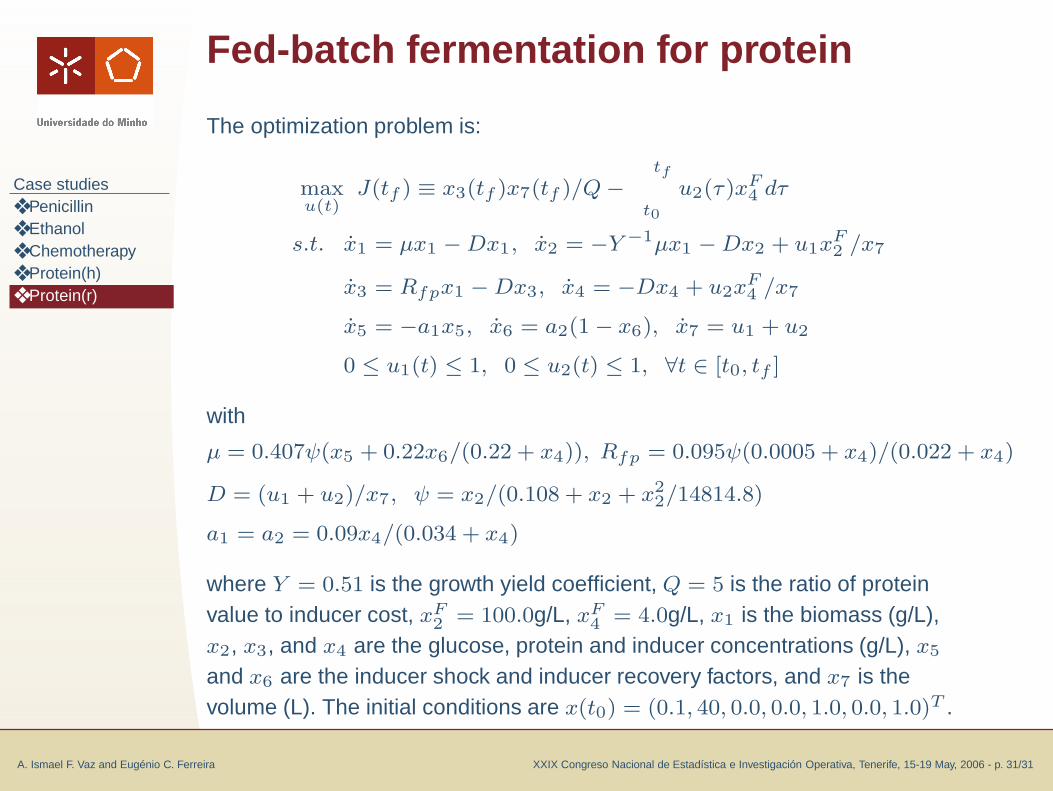
where Y = 0.51 is the growth yield coefficient, Q = 5 is the ratio of proteinvalue to inducer cost, xF
2 = 100.0g/L, xF4 = 4.0g/L, x1 is the biomass (g/L),
x2, x3, and x4 are the glucose, protein and inducer concentrations (g/L), x5
and x6 are the inducer shock and inducer recovery factors, and x7 is thevolume (L). The initial conditions are x(t0) = (0.1, 40, 0.0, 0.0, 1.0, 0.0, 1.0)T .