Optimal Crop Planning and Conjunctive Use ofWater Resources in a Coastal River Basin
LAXMI NARAYAN SETHI1, D. NAGESH KUMAR2∗, SUDHINDRA NATHPANDA1 and BIMAL CHANDRA MAL1
1 Agricultural and Food Engineering Department, Indian Institute of Technology,Kharagpur-721302, India2 Civil Engineering Department, Indian Institute of Science, Bangalore 560012, India(∗ author for correspondence)
(Received: 25 June 2001; accepted: 2 March 2002)
Abstract. Due to increasing trend of intensive rice cultivation in a coastal river basin, crop planningand groundwater management are imperative for the sustainable agriculture. For effective manage-ment, two models have been developed viz. groundwater balance model and optimum cropping andgroundwater management model to determine optimum cropping pattern and groundwater allocationfrom private and government tubewells according to different soil types (saline and non-saline), typeof agriculture (rainfed and irrigated) and seasons (monsoon and winter). A groundwater balancemodel has been developed considering mass balance approach. The components of the groundwaterbalance considered are recharge from rainfall, irrigated rice and non-rice fields, base flow from riversand seepage flow from surface drains. In the second phase, a linear programming optimization modelis developed for optimal cropping and groundwater management for maximizing the economic re-turns. The models developed were applied to a portion of coastal river basin in Orissa State, Indiaand optimal cropping pattern for various scenarios of river flow and groundwater availability wasobtained.
Key words: groundwater balance, linear programming, optimum cropping, salinity and permissiblemining allowance, water resources management
1. Introduction
In view of the ever-increasing human population, intensive rice cultivation andnon-availability of canal water in the coastal humid regions of eastern India, thegroundwater resources are under high pressure of deterioration in quantity andquality. The deterioration of the groundwater quality is the result of intrusion ofseawater into the aquifers due to lowering of fresh groundwater level caused by ex-cessive groundwater abstraction. Due to increasing water scarcity, greater attentionis being given to water management in irrigated as well as in rainfed agriculture.A farmer at the start of each irrigation season needs to have optimum croppingpattern and irrigation programs, which will maximize the economic return. Underthese circumstances there is an urgent need to introduce efficient techniques in land
146 LAXMI NARAYAN SETHI ET AL.
and water resources management for optimal utilization of the available land andwater resources.
A number of simulation and optimization models have been applied in the pastto decide planning and operating strategies for irrigation reservoir systems (Kumarand Pathak 1989; Vedula and Mujumdar, 1992). Rao et al., (1990) developed amodel for optimal weekly irrigation scheduling policy for two crops by consideringboth seasonal as well as intra seasonal competition for water. Vedula and NageshKumar (1996) developed a mathematical programming model to determine thesteady state optimal operating policy and the associated optimal crop-water al-locations to all the crops for a single purpose irrigation reservoir, combining linearprogramming in the intraseasonal period and stochastic dynamic programming ininter seasonal period.
Most farming situations are concerned with several crops grown in the sameseason. Both allocations of land and water resources under a multi-crop situationin a season should be considered (Paul et al., 2000). Paul et al., (2000) developedoptimal resources allocation strategies for a canal command in the semiarid regionof India in a stochastic regime, considering the competition of crops in a season,both for irrigation water and area of cultivation.
The development of optimization models for improved water management ex-panded rapidly in the last decade. Linear programming is used for multiple cropmodels and dynamic programming for a single crop model. In irrigated agricul-ture, where various crops are competing for a limited quantity of land and waterresources, linear programming is one of the best tools for optimal allocation of landand water resources (Smith, 1973; Maji and Heady, 1980; Loucks et al., 1981;Yaron and Dinar, 1982: Pleban, et al., 1983; Tyagi and Dhruva Narayana, 1984;Chavez-Morales, et al., 1987; Loftis and Houghtalen 1987; Sritharan, et al., 1988;Afshar and Marino, 1989; Mayya and Prasad, 1989; Paudyal and Gupta, 1990;Kaushal, et al., 1985; Panda et al., 1996; Sethi, 2001).
In recent years considerable attention has been given to problems associatedwith groundwater management and salinity control. Groundwater management hasbeen studied from different view points, e.g., the economic control of groundwatermanagement under institutional restrictions (Burt, 1970), the conjunctive manage-ment of groundwater and surface water (Cummings and Winkle, 1974, Khepar andChaturvedi, 1982, Panda et al., 1985) and groundwater management and salinitycontrol (Cummings and Winkle, 1974, Hallaji and Yazicigil, 1996).
Water resources management is generally done by water balance for crop plan-ning. In the present study the optimal cropping pattern and area allocation withrespect to availability of water resources (both surface and groundwater) wereobtained for different seasons by developing an optimization model. Water balancemodel has also been developed using the methods of Satish Chandra and Saxena(1975) and Panda et al. (1996) considering mass balance approach. In addition tothe rational water use, there is need for selecting economically viable croppingpattern for a given area with available resources. Such cropping pattern can be
OPTIMAL CROP PLANNING AND CONJUNCTIVE USE OF WATER RESOURCES 147
obtained through the use of optimization models. The optimal cropping pattern wasobtained for different soil types (saline and non-saline), type of agriculture (rainfedand irrigated) and seasons (monsoon and winter) using Linear Programming (LP)model. The objective of the LP model is to find the maximum annual net returnfrom different cropping patterns and areas for all types of agriculture (rainfedand irrigated) under different soil types. This optimization is subject to variousconstraints such as surface and groundwater availability and their mass balance,cropping pattern restrictions. These models were applied to a portion of coastalriver basin in Orissa State, India. The study was undertaken with a view to assist intaking decisions about crop planning and groundwater management.
2. Study Area
The study area, a portion of coastal river basin in India, is situated within the northlatitude of 21◦27′ 0′′ to 21◦45′ 45′′ and east longitude of 86◦56′ 15′′ to 87◦20′30′′ spanning over an area of 1066 square kilometers, out of which 833.15 squarekilometers is cultivable land (Figure 1). The area is situated in three administrativeblocks, namely, Balasore Sadar, Basta and Baliapal of Balasore district in OrissaState, India.
The study area is bounded on the north and the south by two rivers (Subarn-arekha and Budhabalang), on the east by Bay of Bengal and on the west by hillyareas of Mayurbhanj district of Orissa State. The area can be categorized into threedistinct morphological units viz. saline marshy tract along the coast, the gentlyslopping alluvial plain in the central part and the hilly region in the western parts.The saline marshy tract forms a long and narrow strip along the coast. The width ofthis tract varies from 3 to 5 km and is intersected by a good number of tidal streamsand is covered by shrubby vegetation. The gently sloping alluvial plain is situatedto the west of the saline marshy tract and is the most fertile part of the area. Thegeneral slope of this tract is towards east and southeast and varies from 0.57 to 1.33m per km. The hilly region in the western part is an extension of the Eastern Ghatsmountain range. These hill ranges are trending roughly in the northeast-southwestdirection. The maximum elevation in this region is 40 m above mean sea level.The climate of the area is characterized by tropical monsoon climate having threedistinct seasons viz. monsoon, winter and summer. The average annual rainfall ofthe region varies between 1500–2000 mm, two third of which occurs in monsoonseason between mid-June and mid-September. During this period, a large volumeof rainwater from the rice fields discharges into the sea through surface drainsand rivers. In this process, a huge quantity of fertile soil nutrients and appliedfertilizers are drained into the sea. A study of the existing cultivation practicesreveals that the farmers usually grow crops in two seasons (monsoon and winter)in both rainfed and irrigated areas. Farmers normally grow rice as a principalcrop. Apart from rice, pulses, oilseeds and vegetables are the other crops grownduring monsoon and winter seasons. In summer season there is no cultivation in
148 LAXMI NARAYAN SETHI ET AL.
Figure 1. Location map of study area.
the area. In the various seasons the cropping area does not remain the same. Thisis due to the uncertainty of rainfall, scanty water resources, uncontrolled grazingof animals, management problems due to considerable distance from the farmers’houses, theft possibilities of high valued crops and other socio-economic problems.The only sources of water available for irrigation are the groundwater and the riverwater from Subarnarekha and Budhabalang. In the study area, no canal irrigationsystem is available. The structures used for irrigation are the government owneddeep tubewells (more than 60 m) and private shallow (less than 20 m) and mini-deep tubewells (between 20 and 60 m) and river lifts. Cost of groundwater fromgovernment owned deep tubewells (here afterwards referred as government tube-
OPTIMAL CROP PLANNING AND CONJUNCTIVE USE OF WATER RESOURCES 149
wells) is subsidized by the state government. Therefore, groundwater abstraction isintensive in the rice-cultivated areas. If the present increasing trend of groundwaterabstraction continues, it may further lead to decline in groundwater table, seawaterintrusion, and non-functioning of shallow tubewells operated by centrifugal pumps.So, a farmer at the start of each irrigation season needs to have optimum croppingpattern and irrigation program to maximize his economic returns.
3. Model Development
Two models, viz. groundwater balance model and optimum cropping and ground-water management model are developed to determine the optimum cropping pat-tern and groundwater allocation corresponding to different soil type (saline andnon-saline), type of agriculture (rainfed and irrigated) and seasons (monsoon andwinter).
3.1. GROUNDWATER BALANCE MODEL
Groundwater balance is an important aspect of any study on allocation of waterresources, planning and management. The objective of the groundwater balancemodel is to regulate the groundwater flow system so as to prevent the water tablefrom rising too close and/or declining too far from the root zone of the crops. Thisamounts to increasing or reducing the groundwater discharge at different locationsas per requirement. The simplest form of groundwater balance equation is givenby:
�S = TGRr – TGDd (1)
in which �S = change of groundwater storage, m3; TGRr = total groundwaterrecharge, m3; and TGDd = total groundwater draft, m3.
3.1.1. Groundwater Recharge
Groundwater recharge consists of recharge from rainfall, seepage flow from surfacedrains, base flow from rivers, deep percolation from irrigated rice and non-riceareas. However, seepage from field drainage channels and conveyance system hasbeen neglected. The annual groundwater recharge (starting of monsoon season toend of winter season) has been estimated by using the following equation:
TGRr = Rr + GRp + GRnp + BF + SF (2)
in which Rr = recharge to the groundwater from rainfall, m3; GRp = recharge tothe groundwater from irrigated rice area, m3; GRnp = recharge to the groundwaterfrom irrigated non-rice area, m3; SF = seepage flow to the study area from drains,m3; and BF = base flow to the area from the rivers, m3.
150 LAXMI NARAYAN SETHI ET AL.
Recharge from Rainfall
To compute the recharge from rainfall, ten years monthly rainfall data of the studyarea was collected from the Central Water Commission office, Balasore, Orissa.Annual groundwater recharge (cm) from rainfall in cm was calculated using thefollowing equation given by Satish Chandra and Saxena (1975).
Rr = 3.984(Rav – 40.64)0.5 (3)
in which Rav = average annual rainfall of the area, cm.
Recharge from Irrigated Fields
Recharge from irrigated fields including losses in field channels was estimated us-ing the norms recommended by the Groundwater Estimation Committee (1984) asfollows. The different percentages of seepage and percolation in crop fields adoptedare based on the studies conducted in similar areasa) Recharge from irrigated rice area (GRp): 35 to 64% of tubewell dischargeb) Recharge from irrigated non-rice area (GRnp): 30 to 36% of tubewell dis-
chargeIn the present study recharge from tubewells and from river lift irrigated fields
(including losses in field channels) for rice and non-rice fields are taken as 55 and30%, respectively.
Base Flow from Rivers
In the present study, the major groundwater recharge contribution is the base flowfrom Subarnarekha and Budhabalang rivers. Until recently, the common methodsused for estimation of base flow are direct-measurement method, the curve tangentmethod, the basin area method and the chemical and isotope method (Delleur,1998). In the present study, direct-measurement methodology has been used forestimation of the base flow from rivers, where an accurate estimate of hydraulicconductivity of the soils of the riverbeds was obtained using Falling Head Per-meameter method in the laboratory. The Darcy’s law was used to estimate the baseflow from rivers considering the annual average groundwater flow gradient on bothsides of the rivers and the cross-sectional area through which flow takes place.
Seepage Flow from Drains
Seepage from drains depends on factors like seepage rate, wetted perimeter, lengthof drains contributing to seepage and the number of days water remains in thedrains. Due to unavailability of data related to estimation of the seepage fromdrains, it was computed considering run off available in drains as 40% of thetotal rainfall (Sarma et al., 1983). Seepage flow from drains to groundwater wasassumed as 8% of the total run off available in drains (Satish Chandra and Saxena,1975).
OPTIMAL CROP PLANNING AND CONJUNCTIVE USE OF WATER RESOURCES 151
Table I. Existing seasonal water resources systems and the extraction from the water resources
Name of Structures Number Average Operating Total draft (Mm3)
Source: Lift Irrigation Corporation, Balasore, Orissa, India.Note: Figures in the parenthesis indicate number of structures in saline area.
3.1.2. Groundwater Discharge
Groundwater discharge consists of draft from tubewells and evaporation from ground-water, which is given by:
TGDd = GDt + GDe (4)
in which GDt = groundwater draft from tubewells, m3; GDe = evaporation fromgroundwater, m3.
Groundwater Draft
Private shallow and mini-deep tubewells and government deep tubewells in thestudy area are being used for pumping the groundwater. The number of tubewellsvaries in different years. The year-wise groundwater draft is based on discharge,number of wells and duration of operation of wells in each season (Table I).
Evapotranspiration from Groundwater
Evapotranspiration from groundwater is difficult to be evaluated. In the study areathe average groundwater level varies from 3 to 9 m below surface. The evapotran-spiration from groundwater is assumed negligible due to high depth of water tablefrom the surface and absence of deep-rooted forest plants.
152 LAXMI NARAYAN SETHI ET AL.
3.2. OPTIMAL CROPPING AND GROUNDWATER MANAGEMENT MODEL
The objective of the model is to maximize the net annual return from the studyarea considering the returns from crop but excluding the irrigation cost. The de-cision variables of the models are seasonal area allocation to crops and surfacewater and groundwater application for crop production. The rainfall and irrigationrequirement of crops, which are inputs to the model, are considered as stochasticvariables.
3.2.1. Objective Function
The objective function consists of maximizing the net annual return (Z) from thecoastal river basin subject to constraints on the availability of water and otherinputs.
MaxZ =2∑i=1
2∑j=1
2∑k=1
n∑c=1
aijkcAijkc −2∑i=1
2∑j=1
2∑k=1
[CRWijk RWijk + (1 + Lr)
(CGW
P
ijk GWPijk + CGW
G
ijk GWGijk
)](5)
in which i = soil type, i = 1 for coastal saline soil and i = 2 for inland non-salinesoil; f = type of agriculture, j = 1 for rainfed agriculture and j = 2 for irrigatedagriculture; k = crop growing season, k = 1 for monsoon season, and = k = 2 forthe winter season; c = 1,2. . ., n; n = number of crops; aijkc = net return (excludingthe cost of irrigation water) for crop c grown in season k of jth type of agriculturein soil type i (Rs ha−1) (US $1 ≈ Indian Rupees, Rs. 48); Aijkc = area allocated tocrop c grown in season of k of jth type of agriculture in soil type i (ha); CRW
ijk = costof lifting river water (RW) in season k for jth type of agriculture in soil type i (Rsha-m−1); RWijk = river water allocated in season k for jth type of agriculture in soiltype i (ha-m); CGWP
ijk = cost of groundwater from private tube well (P) in seasonk for jth type of agriculture and in soil type i (Rs ha-m−1); GWP
ijk = groundwaterpumped from private tube wells in season k for jth type of agriculture in soil typei (ha-m); CGWG
ijk = cost of groundwater from government tube well (G) in seasonk for jth type of agriculture and in soil type i (Rs ha-m−1); GWG
ijk = groundwaterpumped from government tube well in season k for jth type of agriculture in soiltype i (ha-m); and Lr = leaching requirement (fraction).
3.2.2. Constraints
Maximization of the objective function is subject to the following constraints.1. Water Allocation ConstraintThe expected irrigation requirements of all the crops must be fully satisfied duringall the seasons from the available surface and groundwater resources and rainfall
OPTIMAL CROP PLANNING AND CONJUNCTIVE USE OF WATER RESOURCES 153
for both rainfed and irrigated agriculture of the coastal saline and non saline soilareas.
2∑i=1
2∑j=1
n∑c=1
NIRijkcAijkc −2∑i=1
2∑j=1
α1(β1RWijk +
+ GWPijk + GWG
ijk) ≤ 0 for all k; (6)
in which NIRijkc = net irrigation requirement of crop c, grown in season k forjth type of agriculture in soil type i (m); α1 = (1-θ2) = field water applicationefficiency (fraction); θ2 = field water application loss (fraction); β1 = (1-θ1) =conveyance efficiency of river lift system (fraction); and θ1 = conveyance loss ofriver lift system (fraction);
2. Land Area ConstraintLand allocated to various crops during the monsoon and winter seasons must notexceed the available cultivable area for all types of agriculture and the soil types.
2∑i=1
2∑j=1
n∑c=1
Aijkc ≤ TAk for all k (7)
in which TAk = total land area available in season k (ha);
3. Water Availability ConstraintsThe availability of water for irrigation from the surface water source is limited. Soallocation of surface water must not exceed the available surface water during aseason. Similarly for groundwater resources, tube well water allocation must notexceed the availability of groundwater during the season for the corresponding typeof agriculture and also the type of soil.(a) River Water
2∑i=1
2∑j=1
RW ijk ≤ ARWk for all k (8)
(b) Groundwater
2∑i=1
2∑j=1
(1 + Lr)(GWPijk +GWG
ijk) ≤ AGWk for all k (9)
in which ARWk = total available river water in season k after allowing for losses(ha-m); and AGWk = total available groundwater in season k after allowing forlosses (ha-m).
154 LAXMI NARAYAN SETHI ET AL.
Figure 2. Flow chart of groundwater balance for the study area.
4. Hydrologic Balance of aquiferThe proper hydrologic balance of groundwater aquifer will help in keeping thewater table at balanced position. Thus a hydrologic balance constraint should besatisfied (Figure 2).
Neglecting run-off, seepage from field drainage channels and evaporation lossesand rainfall contribution to the water delivery systems during conveyance, thefollowing expression is obtained.
2∑i=1
2∑j=1
2∑k=1
[(GWP
ijk +GWGijk)− {
θ1RWijk + θ3E(R)Aijk+
θ2(β1RWijk +GWPijk +GWG
ijk
)} − BF − SF] ≤ PMA (10)
By rearranging
2∑i=1
2∑j=1
2∑k=1
[(1 − θ2)(GW
Pijk +GWG
ijk)− (θ1 + θ2β1)RWijk
] ≤
[PMA + BF + SF + θ3E(R)Aijk
](11)
OPTIMAL CROP PLANNING AND CONJUNCTIVE USE OF WATER RESOURCES 155
in which θ3 = rainfall recharge (fraction); E(R) = expected annual rainfall (m); SF= seepage loss to the study area from the drain (ha-m); BF = seepage loss to thestudy area from the river (ha-m); PMA = permissible annual mining allowance ofthe aquifer (ha-m); and A = cultivable area under considerations (ha).Permissible annual mining allowance is determined as follows:
PMA = �h× A× Y (12)
in which �h = permissible annual average groundwater table fluctuations (m); andY = specific yield of aquifer (fraction).
5. Minimum/Maximum Allowable AreaManagement considerations restrict some minimum and/or maximum value forirrigated areas under certain crops to meet the local food requirement.a) For Maximum area
Aijkc ≤ µmaxijkcT Aijkc (13-a)
b) For Minimum area
Aijkc ≥ µminijkcT Aijkc (13-b)
in which µmaxijkc = factor by which existing area of crop c can be increased in season
k for jth type of agriculture and soil type i; µminijkc = factor by which existing area of
crop c can be decreased in season k for jth type of agriculture and soil type i andTAijkc = area of crop c as per existing pattern in season k for jth type of agricultureand soil type i (ha).
6. Non-negativity
Aijkc ≥ 0; RW ijk ≥ 0; GWPijk ≥ 0; andGWG
ijk ≥ 0 for all i, j, k, and c (14a-d)
4. Estimation of Model Inputs
The model inputs include determination of the water resources data, leaching frac-tion, net irrigation requirement of crops at different probability of exceedances, netreturn of crops and permissible mining allowance.
4.1. WATER RESOURCES
In the study area, the sources of water available for irrigation purpose are riverwater and groundwater. Although the river water is of good quality, it falls short ofthe irrigation requirement of the area adjoining the river due to very few river lift-pumping units installed by government. The average electrical conductivity of the
156 LAXMI NARAYAN SETHI ET AL.
groundwater is 3.75 dS m−1 (deci Siemen/meter) in the saline area. The structuresused for irrigation are the river lifts and government owned tubewells and private(shallow and mini deep) tubewells. The river water is supplied through 37 river liftirrigation schemes in the study area, which are programmed for different seasons(monsoon and winter) and soil type (saline and non-saline) according to demand.Details of river lift and groundwater pumping sources are given in Table I.
4.2. LEACHING REQUIREMENT
The upper aquifer of coastal saline area is of poor quality not suitable for irrigationwhereas deeper aquifer is suitable for all purposes due to which all the mini-deepand deep tubewells are installed in the said layer. The leaching requirement (Lr)can be calculated based upon the electrical conductivity of irrigation water in saltaffected areas (ECiw) and threshold value of the electrical conductivity of irrigationwater (ECth) for crop tolerance as follows:
Lr = ECiw
ECth(15)
in which ECiw = electrical conductivity of irrigation water (dS m−1); and ECth =threshold electrical conductivity of water draining from the root zone (dS m−1).
4.3. IRRIGATION REQUIREMENT OF CROPS
Crops grown in study area during monsoon season are rice (Oryza sativa), maize(Zea mays), sweet potato (Ipomoea batatas) and pigeon pea (Cajanus cajan) whereaswinter season crops are rice, wheat (Triticum aestivum), groundnut (Arachis hy-pogaea), mustard (Brassica juncea), black gram (Phaseolus mungo), green gram(Phaseolus aureus), onion (Allium cepa), and garlic (Allium sativum).
Various methods are available to estimate the reference crop evapotranspiration(ETo) (Doorenbos and Pruitt, 1977; Allen et al., 1998). Based on the availability ofmeteorological data of the study area, the Hargreaves and Samani (1985) methodof estimating ETo was selected as given below:
ETo = 0.0135Rsl (Tmean + 17.8) (16)
in which ETo = reference evapotranspiration in a given period (month) (mm/month);Rsl = incoming short-wave solar radiation in the considered period (mm/month);Tmean = mean temperature (Tmax + Tmin)/2; Tmax = monthly maximum air temper-ature (◦C); Tmin = monthly minimum air temperature (◦C).
Rsl = 0.16Ra(Tmax − Tmin)0.5 (17)
in which Ra = extra terrestrial solar radiation (mm/month).
OPTIMAL CROP PLANNING AND CONJUNCTIVE USE OF WATER RESOURCES 157
Now, the crop evapotranspiration (ETc) is calculated using the following equa-tion,
ETc = kcETo (18)
where, kc = crop coefficient.The crop coefficient (kc) values for each crop were obtained from literature
(Doorenbos and Pruitt, 1977 and Allen et al., 1998). The U.S. Department ofAgriculture (USDA) Soil Conservation Service (SCS) method (Dastane, 1977) wasused to determine the effective rainfall. The total depth of net irrigation requirementof crop that needs to be applied to meet the crop demand can be estimated from thefollowing equation:
NIR = ETc − ER (19)
in which NIR = net irrigation requirement in a given month, mm/month; and ER =effective rainfall in the given month, mm/month;
The seasonal net irrigation requirement (NIR) of crops has been computed byadding the monthly NIR of crops corresponding to the months in the growingseason.
4.4. PROBABILITY OF EXCEEDANCE (PE)
The daily rainfall and temperature of the study area for 10 yr (1991–2000) wascollected and converted to monthly values. These values were used to predict theexpected monthly rainfall and evapotranspiration at different probability levels.The values were entered in the database of SMADA package (Statistical Modelfor Analysis of Distribution function) considering Weibull’s distribution as ref-erence and fitted to different probability functions. From the best-fit distribution(in this case, normal distribution), the value of the monthly-expected referenceevapotranspiration at 10, 20, 30, 40, 50, 60, 70, 80, and 90% probability levelscould be obtained. Based on these values, the net irrigation requirements (NIR) ofcrops at various probability levels of exceedance (PE) were computed for both thegrowing seasons, and are shown in Figures 3 and 4 for monsoon season and winterseason respectively. The optimal annual returns at different probability levels ofNIR and the optimal groundwater allocation are computed by assuming that all thecomponents of the groundwater balance taken in the calculations are correct.
4.5. NET RETURNS OF CROPS
The net return from the cultivation of selected crops per unit area of farming wascalculated by considering the potential yield from the crops. The variation of netreturn excluding irrigation water cost depends upon the type of soil, agriculture andthe crops with their corresponding yield, market price and the cost of cultivation.
158 LAXMI NARAYAN SETHI ET AL.
Figure 3. Variation of net irrigation requirement of crops with different probability ofexceedance level during monsoon season.
The potential yield values of the study area were collected from the Agriculture De-partment, Government of Orissa. The cost of production of various crops excludingthe cost of irrigation water was obtained from the budget for monsoon and wintercrops suggested by the Department of Statistics and Economics, Orissa, India. Thenet returns excluding the irrigation water cost for crop c, season k, agriculture typej and soil type i were determined based on these inputs (Table II).
4.6. PERMISSIBLE MINING ALLOWANCE
Permissible mining allowance (safe yield) is the upper limit of groundwater pump-ing without creating adverse effect on groundwater management. Adverse effectmay be either declining or rising of groundwater table or intrusion of poor qualitywater either from sea (salt water intrusion) or from adjoining aquifer due to creationof adverse flow gradients. The groundwater should be managed so that the aver-age depletion does not exceed the permissible mining allowance. The permissiblemining allowance (PMA) is calculated using Equation 12.
OPTIMAL CROP PLANNING AND CONJUNCTIVE USE OF WATER RESOURCES 159
Figure 4. Variation of net irrigation requirement at different probability of exceedance levelduring winter season.
5. Model Application
The coastal river basin is divided into the saline and non-saline areas based on thegeography and the salinity of the soil. The total cultivable area (TAijkc) for salinewhen i = 1 and non-saline when i = 2 are 60 and 773.15 sq. Km, respectively.The cultivable area is categorized into rainfed and irrigated according to the typeof agriculture. Finally the cropping pattern was decided based on the cultivationseason, soil and agriculture type. The existing cropping pattern and correspondingnet returns excluding the irrigation water cost for crop c, season k, agriculture typej and soil type i of the study area are shown in Table II. The unit cost of irriga-tion water supply through the government owned riverlifts (CRW
ijk ) and tubewells
pumping units (CGWG
ijk ) is Rs. 1,715.55/ha-m−1 and for privately owned shallow
and mini-deep tubewells (CGWP
ijk ) is Rs. 3,333.30 ha-m−1. The supplies of riverwater during monsoon and winter seasons (ARWk) are 43.55 and 653.18 Mm3,respectively. Water samples from all the tubewells were analyzed. The electricalconductivity of groundwater varied from 0.60 to 1.42 dS m−1, with an average of1.00 dS m−1 in non-saline area and 3 to 4.5 dS m−1 with an average of 3.75 dS m−1
in saline area. For most of crop in the study area salinity tolerance is 6 dS m−1. The
160 LAXMI NARAYAN SETHI ET AL.
Table II. Existing cropping pattern and net return excluding irrigation cost
Soil Agriculture Seasons Crops Area Yield Cost of Net return
Type (i) (j) k) (c) (ha) (1000 kg cultivation (excluding
Source: District Agriculture Office, Balasore, Orissa, India.a US $1 ≈ Rs. 48.
leaching requirement (Lr ) of the saline area was found to be 0.625, whereas for thenon-saline area it is zero.
Water balance components were computed using the methods described earlierand norms, which are based on field experiments. The results show the rechargefrom different components of water balance, drafts from the groundwater struc-
OPTIMAL CROP PLANNING AND CONJUNCTIVE USE OF WATER RESOURCES 161
Table III. Annual groundwater balance obtained from the groundwater balance model
Items Million m3
Inflow to the groundwater basin
Recharge from rainfall 258.49
Recharge from river lifts and tube-wells irrigated rice area 85.15
Recharge from river lifts and tube-wells irrigated non-rice area 41.29
Base flow from Subarnarekha and Budhabalang rivers 508.78
Seepage from drains 43.25
Total inflow to the ground water basin 936.96
Evaporation from ground water Negligible
Seepage to rivers and drains from groundwater as sub-surface out flow Negligible
Ground water available 936.96
Usable groundwater (70% of available) 655.87
Groundwater draft from tube wells 255.03
Net groundwater resources to be developed 400.84
tures, the usable water resources and the net groundwater resources to be tappedfor further development.
The total annual average groundwater recharge of the study area have been com-puted as 936.96 Mm3 (million cubic meters) which includes annual recharge fromrainfall [θ3E(R)Aijk] as 258.49 Mm3, base flow from rivers (BF) as 508.78 Mm3,seepage flow from surface drains (SF) as 43.25 Mm3, and discharge as 255.03Mm3 (Table III). The annual groundwater available (AGWk) is 655.87 Mm3. Thepermissible mining allowance (PMA) was found as 231.795 Mm3. The conveyanceloss of river lift system (θ1) and field water application loss (θ2) assumed is 0.2 and0.3 (fraction), respectively (Panda et al., 1996 and Sethi, 2001).
6. Optimum Resources Allocation
Optimization model (Linear programming) developed for optimum cropping pat-tern and groundwater management consisted of 35 decision variables out of which25 variables correspond to crop variables and 10 correspond to water resources.The optimization model was run for nine different probability levels of exceedance(10, 20, 30, 40, 50, 60, 70, 80 and 90) of net irrigation requirements using QSBpackage (Chang, 1993). The model was also run for three different cropping situ-ations viz., Case 1: Without Area Constraints i.e. there are no lower and upperbounds on the area cultivated for each crop (in this case µmin
ijkc = 0 and µmaxijkc = 1 for
all i, j, k and c) Case 2: With rice area constraints i.e. rice cultivation is restrictedto existing rice area while there are no bounds on all other crops. This alternative
162 LAXMI NARAYAN SETHI ET AL.
Figure 5. Optimal annual return with different probability of exceedance of NIR.
was examined since rice cultivation is essential for the farmers of the area for theirfood requirement even if it is not economical. Case 3: Existing cropping pattern.The optimal annual return obtained for different net irrigation requirements (NIR)corresponding to different probability levels of excedance is shown in Figure 5.Groundwater allocations from government tubewell for all the three cases at differ-ent levels of exceedance of NIR are shown in Table IV. As can be seen from Figure5 and Table IV, there is very little variation in optimal annual return and ground-water allocation obtained for different NIR corresponding to different probabilitylevels of exceedance. Therefore for further analysis, net irrigation requirementscorresponding to 90% probability of exceedance is only considered.
The cropping pattern obtained from the optimum cropping and groundwatermanagement model for the above three different cropping situations (case 1, 2 and3) is presented in Table V considering NIR at 90% exceedance probability. For case1, the crops with most economic benefit are preferred for cultivation in the entirearea. They are sweet potato in monsoon season and groundnut in winter season.Although these may yield maximum annual return it may not be feasible due tothe local food requirements. The results obtained for case 2, when a constraint isimposed for a minimum rice area as per the existing cropping pattern, are alsoshown in Table V. Annual return for the existing cropping pattern (case 3) is alsoshown in the same table.
No data is available from the study area regarding the minimum requirementsof crops for the farmers as well as the food targets of the region. So, the model wasrun at three different ranges of the cultivable area considering the existing croppingpattern.
OPTIMAL CROP PLANNING AND CONJUNCTIVE USE OF WATER RESOURCES 163
Table IV. Optimum groundwater allocation at different probability levels of exceedance ofNIR corresponding to different cases of cropping situation
Probability Groundwater allocation through government tubewell (Thousand ha-m)
level of Case 1 Case 2 Case 3
exceedance
Monsoon Winter Monsoon Winter Monsoon Winter
90 14.28 22.260 19.750 25.690 19.710 25.760
80 4.998 21.889 10.700 25.369 10.659 25.376
70 0 20.947 4.069 24.514 4.074 24.486
60 0 19.757 2.092 23.389 2.092 23.334
50 0 18.567 0.233 22.296 0.232 22.255
40 0 17.258 0 21.084 0 21.069
30 0 15.829 0 19.753 0 19.759
20 0 14.045 0 18.032 0 18.065
10 0 11.426 0 15.577 0 15.667
These ranges are (1) Allowing 20% deviation from the existing area for eachcrop i.e. µmin
ijkc = 0.8 and µmaxijkc = 1.2 for all i, j k and c. (2) Allowing 40% deviation
from the existing area for each crop i.e. µminijkc = 0.4 and µmax
ijkc = 1.6 for all i, j k andc. (3) Allowing 50% deviation from the existing area for each crop i.e. µmin
ijkc = 0.5and µmax
ijkc = 1.5 for all i, j, k and c. It may be noted that the total cropped area isrestricted to the total cultivable area (Equation 7) in the model. Fifty percent of theexisting cropped area is considered as the minimum required area to be cultivatedfor each crop. Therefore, deviations below 50% are not considered. Optimal crop-ping pattern obtained for the above three different ranges of the cultivable area withreference to existing cropping pattern are shown in Table V. It can be observed fromthe table that with the increase in allowable deviation from the existing croppingpattern more economic benefit is obtained. These alternative cropping patterns maybe adopted as per the desire of the farmers to change their cropping pattern.
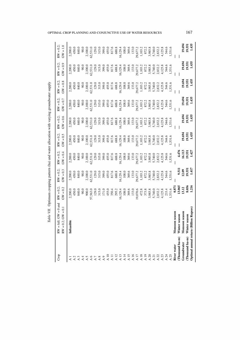
The optimum cropping and ground water management model was also runvarying the surface and ground water availability at different levels (10% inter-vals) considering the existing potential fully utilized. The cropping pattern, waterresources allocation with maximum annual net return obtained with varying sur-face and groundwater availability are presented in Tables VI and VII, respectively.Optimum annual return obtained for different levels of surface and groundwateravailability are also shown in the tables.
164 LAXMI NARAYAN SETHI ET AL.
Tabl
eV.
Opt
imum
area
and
grou
ndw
ater
allo
cati
onco
rres
pond
ing
toth
ree
crop
ping
situ
atio
nsan
dde
viat
ion
rang
esfr
omth
eex
isti
ngcr
oppi
ngpa
tter
n
Soil
type
Agr
icul
ture
Seas
onC
rop
Opt
imal
area
allo
catio
n(h
a)
Sym
bol
Cas
e1
Cas
e2
Cas
e3
Ran
geof
the
culti
vabl
ear
eaco
rres
pond
ing
toex
istin
gar
ea
(Aijkc)
Ran
ge1
Ran
ge2
Ran
ge3
Salin
eR
ainf
edM
onso
onR
ice
A1
0.0
3700
.037
00.0
2960
.022
20.0
1850
.0
Mai
zeA
20.
00.
075
0.0
600.
045
0.0
375.
0
Irri
gate
dM
onso
onR
ice
A3
0.0
1400
.014
00.0
1120
.084
0.0
700.
0
Mai
zeA
40.
00.
015
0.0
120.
090
.075
.0
Win
ter
Ric
eA
50.
015
00.0
1500
.018
00.0
2100
.022
50.0
Non
-Sal
ine
Rai
nfed
Mon
soon
Ric
eA
60.
064
765.
064
765.
063
673.
062
531.
061
960.
0
Mai
zeA
70.
00.
021
5.0
172.
012
9.0
107.
5
Pige
onpe
aA
80.
00.
022
5.0
270.
031
5.0
337.
5
Win
ter
Mus
tard
A9
0.0
0.0
285.
034
2.0
399.
042
7.5
Gro
undn
utA
100.
00.
032
5.0
390.
045
5.0
487.
5
Bla
ckgr
amA
110.
00.
058
4.0
700.
881
7.6
876.
0
Gre
engr
amA
120.
00.
049
2.0
590.
468
8.8
738.
0
Irri
gate
dM
onso
onR
ice
A13
0.0
1152
1.0
1152
1.0
1382
5.2
1612
9.4
1728
1.5
Mai
zeA
140.
00.
018
0.0
144.
010
8.0
90.0
Swee
tPot
ato
A15
8331
5.0
1929
.031
5.0
316.
836
9.6
396.
0
Pige
onpe
aA
160.
00.
095
.011
4.0
133.
014
2.5
Win
ter
Ric
eA
170.
021
198.
021
198.
025
437.
629
677.
231
797.
0
Whe
atA
180.
00.
078
8.0
945.
611
03.2
1182
.0
Mai
zeA
190.
00.
062
3.0
747.
687
2.2
934.
5
Mus
tard
A20
0.0
0.0
2847
.034
16.4
3985
.842
70.5
Gro
undn
utA
2183
315.
060
617.
048
220.
049
20.0
5740
.061
50.0
Bla
ckgr
amA
220.
00.
020
23.0
2427
.628
32.2
3034
.5
Gre
engr
amA
230.
00.
029
47.0
3536
.441
25.8
4420
.5
Gar
licA
240.
00.
038
9.0
466.
854
4.6
583.
5
Oni
onA
250.
00.
010
9413
12.8
1531
.616
41.0
Opt
imal
annu
alre
turn
(Bill
ion
Rup
ees)
3.64
2.25
2.11
1.32
1.44
1.49
Gro
undw
ater
allo
cati
onM
onso
onse
ason
14.2
8019
.750
19.7
1019
.687
19.6
9419
.698
(Tho
usan
dha
-m)
Win
ter
seas
on22
.260
25.6
9025
.760
16.7
7019
.550
20.9
50
OPTIMAL CROP PLANNING AND CONJUNCTIVE USE OF WATER RESOURCES 165
7. Summary and Conclusions
Groundwater balance model has been developed using mass balance approach toestimate usable quantity of groundwater in the study area. Different componentsconsidered in this model are recharge from rainfall, irrigated rice fields, irrigatednon-rice fields, base flow from rivers and seepage flow from drains.
The linear programming model for optimization of annual return was formu-lated for optimum water allocation and cropping pattern considering the saline andnon-saline soil type, rainfed and irrigated agriculture and the monsoon and winterseason and different crops. Following specific conclusions can be drawn for thestudy area based on the results obtained from the models.
• The water balance model shows that the additional water resources available(400.84 Mm3) (after withdrawing 255.03 Mm3) for further use is more thanthe present demand due to more recharge from rainfall (258.49 Mm3) and baseflow from rivers (508.78 Mm3).
• The optimum cropping and groundwater management linear programming modelyielded the cropping pattern for three situations. The optimal annual returnsat 90% probability levels of NIR corresponding to three different croppingsituation (Case 1, Case 2 and Case 3) are 3.64, 2.25 and 2.11 billion Rupees,respectively and the optimal value increases with decreasing probability levelsof NIR.
• The optimal groundwater allocation for three different cropping situations at-tains the maximum level at 90% probability level of NIR and decreases withdecreasing probability levels of exceedance of NIR.
• The model when imposed with a constraint of 20% of existing surface andgroundwater supply level, yielded the allocation towards all resources (riverand groundwater) for both the growing seasons.
• The cropping pattern obtained for three different ranges of deviation fromthe existing area for each crop also gives significant output in the form ofalternative cropping pattern.
8. Conclusions
The groundwater balance of a basin was studied considering recharge from rainfall,irrigated rice fields, irrigated non-rice fields, base flow from rivers and seepage flowfrom drains and drafts through different groundwater structures like governmentdeep tube wells, private shallow and mini deep tube wells. The linear programmingmodel formulated for maximization of annual net return with optimal water andcropping pattern allocation considering the saline and non-saline soil type, rainfedand irrigated agriculture and the monsoon and winter seasons and the crops isfound to be an effective tool for land and water resources allocation. State agenciesand farmers involved in the actual agricultural production processes are advised topractise conjunctive use of river water and groundwater so as to restrict further de-pletion of groundwater level. However, the result of this study was mainly affected
166 LAXMI NARAYAN SETHI ET AL.
Tabl
eV
I.O
ptim
umcr
oppi
ng(h
a)an
dw
ater
allo
cati
onw
ith
vary
ing
rive
rw
ater
supp
ly
Cro
pG
W=
0.1,
RW
=0.
1;G
W=
0.1,
RW
=0.
2;G
W=
0.1,
GW
=0.
1;G
W=
0.1;
GW
=0.
1;G
W=
0.1;
GW
=0.
1;
RW
=0.
3;G
W=
0.1;
RW
=0.
4;G
W=
0.1,
RW
=0.
5R
W=
0.6
RW
=0.
7R
W=
0.8
RW
=0.
9R
W=
full
A1
Infe
asib
le2,
200.
02,
200.
02,
200.
02,
200.
02,
200.
0A
245
0.0
450.
045
0.0
450.
045
0.0
A3
840.
084
0.0
840.
084
0.0
840.
0A
490
.090
.090
.090
.090
.0A
590
0.0
2,10
0.0
2,10
0.0
2,10
0.0
900.
0A
662
,531
.062
,531
.062
,531
.062
,531
.062
,531
.0A
712
9.0
129.
012
9.0
129.
012
9.0
A8
315.
031
5.0
315.
031
5.0
315.
0A
917
1.0
399.
039
9.0
399.
017
1.0
A10
195.
045
5.0
455.
045
5.0
195.
0A
1135
0.4
817.
681
7.6
817.
635
0.4
A12
295.
268
8.8
688.
868
8.8
295.
2A
1316
,129
.416
,129
.416
,129
.416
,129
.416
,129
.4A
1410
8.0
108.
010
8.0
108.
010
8.0
A15
369.
636
9.6
369.
636
9.6
369.
6A
1613
3.0
133.
013
3.0
133.
013
3.0
A17
12,7
18.8
29,6
77.2
29,6
77.2
29,6
77.2
12,7
18.8
A18
472.
81,
103.
21,
103.
21,
103.
247
2.8
A19
373.
887
2.2
872.
287
2.2
373.
8A
202,
781.
33,
985.
83,
985.
83,
985.
82,
781.
3A
212,
460.
02,
630.
43,
934.
55,
238.
55,
740.
0A
221,
213.
81,
213.
81,
213.
81,
213.
82,
052.
2A
231,
768.
21,
768.
21,
768.
21,
768.
21,
768.
2A
2423
3.4
233.
423
3.4
233.
423
3.4
A25
656.
465
6.4
656.
465
6.4
656.
4R
iver
wat
eral
loca
tion
(Tho
usan
dha
-m)
Mon
soon
seas
on—
——
——
Win
ter
seas
on2.
613.
053.
483.
94.
354
Gro
undw
ater
allo
cati
on(T
hous
and
ha-m
)M
onso
onse
ason
6.55
86.
558
6.55
86.
558
6.55
8W
inte
rse
ason
19.6
9419
.694
19.6
9419
.694
19.6
94O
ptim
alan
nual
retu
rn(B
illio
nR
upee
s)1.
047
1.07
41.
110
1.12
61.
146
OPTIMAL CROP PLANNING AND CONJUNCTIVE USE OF WATER RESOURCES 167
Tabl
eV
II.
Opt
imum
crop
ping
patt
ern
(ha)
and
wat
eral
loca
tion
wit
hva
ryin
ggr
ound
wat
ersu
pply
Cro
pR
W=
full;
GW
=0
and
RW
=0.
2;R
W=
0.2;
RW
=0.
2;R
W=
0.2;
RW
=0.
2;R
W=
0.2;
RW
=0.
2;R
W=
0.2;
RW
=0.
2;
RW
=0.
2;G
W=
0.1
GW
=0.
2G
W=
0.3
GW
=0.
4G
W=
0.5
GW
=0.
6G
W=
0.7
GW
=0.
8G
W=
0.9
GW
=1.
0
A1
Infe
asib
le2,
200.
02,
200.
02,
200.
02,
200.
02,
200.
02,
200.
02,
200.
02,
200.
02,
200.
0A
245
0.0
450.
045
0.0
450.
045
0.0
450.
045
0.0
450.
045
0.0
A3
840.
084
0.0
840.
084
0.0
840.
084
0.0
840.
084
0.0
840.
0A
490
.090
.090
.090
.090
.090
.090
.090
.090
.0A
590
0.0
2,10
0.0
2,10
0.0
2,10
0.0
2,10
0.0
2,10
0.0
2,10
0.0
2,10
0.0
2,10
0.0
A6
57,5
63.0
62,5
31.0
62,5
31.0
62,5
31.0
62,5
31.0
62,5
31.0
62,5
31.0
62,5
31.0
62,5
31.0
A7
129.
012
9.0
129.
012
9.0
129.
012
9.0
129.
012
9.0
129.
0A
831
5.0
315.
031
5.0
315.
031
5.0
315.
031
5.0
315.
031
5.0
A9
171.
039
9.0
399.
039
9.0
399.
039
9.0
399.
039
9.0
399.
0A
1045
5.0
455.
045
5.0
455.
045
5.0
455.
045
5.0
455.
045
5.0
A11
350.
481
7.6
817.
681
7.6
817.
681
7.6
817.
681
7.6
817.
6A
1229
5.2
688.
868
8.8
688.
868
8.8
688.
868
8.8
688.
868
8.8
A13
16,1
29.4
16,1
29.4
16,1
29.4
16,1
29.4
16,1
29.4
16,1
29.4
16,1
29.4
16,1
29.4
16,1
29.4
A14
108.
010
8.0
108.
010
8.0
108.
010
8.0
108.
010
8.0
108.
0A
1536
9.6
369.
636
9.6
369.
636
9.6
369.
636
9.6
369.
636
9.6
A16
133.
013
3.0
133.
013
3.0
133.
013
3.0
133.
013
3.0
133.
0A
1719
,070
.629
,677
.229
,677
.229
,677
.229
,677
.229
,677
.229
,677
.229
,677
.229
,677
.2A
1847
2.8
1,10
3.2
1,10
3.2
1,10
3.2
1,10
3.2
1,10
3.2
1,10
3.2
1,10
3.2
1,10
3.2
A19
373.
887
2.2
872.
287
2.2
872.
287
2.2
872.
287
2.2
872.
2A
203,
985.
83,
985.
83,
985.
83,
985.
83,
985.
83,
985.
83,
985.
83,
985.
83,
985.
8A
215,
740.
05,
740.
05,
740.
05,
740.
05,
740.
05,
740.
05,
740.
05,
740.
05,
740.
0A
222,
832.
22,
832.
22,
832.
22,
832.
22,
832.
22,
832.
22,
832.
22,
832.
22,
832.
2A
234,
125.
84,
125.
84,
125.
84,
125.
84,
125.
84,
125.
84,
125.
84,
125.
84,
125.
8A
2423
3.4
544.
654
4.6
544.
654
4.6
544.
654
4.6
544.
654
4.6
A25
1,53
1.6
1,53
1.6
1,53
1.6
1,53
1.6
1,53
1.6
1,53
1.6
1,53
1.6
1,53
1.6
1,53
1.6
Riv
erw
ater
Mon
soon
seas
on0.
871
——
——
——
——
(Tho
usan
dha
-m)
Win
ter
seas
on13
.065
9.51
14.
476
——
——
——
Gro
undw
ater
Mon
soon
seas
on13
.12
12.0
916
.113
19.6
9419
.694
19.6
9419
.694
19.6
9419
.694
(Tho
usan
dha
-m)
Win
ter
seas
on8.
056
19.5
5119
.551
19.5
5119
.551
19.5
5119
.551
19.5
5119
.551
Opt
imal
annu
alre
turn
(Bill
ion
Rup
ees)
1.21
61.
417
1.42
71.
435
1.43
51.
435
1.43
51.
435
1.43
5
168 LAXMI NARAYAN SETHI ET AL.
by the variation in groundwater pumping, size of the pumping plant, unit cost ofwater, market price of the crops and cost of production.
Acknowledgements
The authors with to sincerely thanks to the Orissa Lift Irrigation Corporation Officeat Jaleshwar and Balasore, District Agriculture Office at Balasore, Central WaterCommission Office at Balasore for providing all necessary data. The financialsupport received from the Volkswagen Foundation, Germany for carrying out theinvestigation is also gratefully acknowledged.
References
Afshar, A. and Marino, M. A.: 1989, ‘Optimization models for wastewater reuse in irrigation’,Journal of Irrigation and Drainage Engineering, ASCE, 115(2), 185–203.
Allen, R. G., Pereira, L. S., Raes, D. and Smith, M.: 1998, Guidelines for Computing Crop WaterRequirements, FAO Irrigation and Drainage Paper 56, Food and Agriculture Organization of theUnited Nations, Rome, Italy, 135 pp.
Burt, C. R.: 1970, ‘Ground water storage control under institutional restrictions’, Water ResourcesResearch 66, 1540–1548.
Chang, Y-L.: 1993, Quantitative Systems for Business Plus, Version 3.0, Prentice Hall, New Jersey,U.S.A.
Chavez-Morales, J., Marino, M. A. and Holzapfel, E. A.: 1987, ‘Planning model of irrigation district’,Journal of Irrigation and Drainage Engineering, ASCE, 113(4), 549–564.
Cummings, R. G. and Winkle, D.: 1974, ‘Water Resources Management in Arid Environments’,Water Resources Research 10(5), 909–915.
Dastane, N. G.: 1977, Effective Rainfall in Irrigated Agriculture, FAO, Irrigation, and Drainage Paperno. 25, Rome.
Delleur, J. W.: 1998, The Hand Book of Groundwater Engineering, CRC Press and Springer-verlag,pp. I 34–35.
Doorenbos, J. and Pruitt, W. O.: 1977, Guidelines for Predicting Crop Water Requirements, FAO,Irrigation, and Drainage Paper no.24, Rome.
Groundwater Estimation Committee: 1984, Norms for Groundwater Assessment, National Bank ofAgriculture and Rural Development, Bombay, India.
Hargraves, G. and Samani, Z. A.: 1985, ‘Reference crop evapotranspiration from temperature’,Transactions, ASAE, 1(2), 96–99.
Hallaji, K. and Yazicigil, H.: 1996, ‘Optimal management of a coastal aquifer in southern Turkey’,Journal of Water Resources Planning and Management ASCE, 122(4), 233–244.
Kaushal, M. P., Khepar, S. D. and Panda, S. N.: 1985, ‘Saline groundwater management and optimalcropping pattern’, Water International 10(2), 86–91.
Khepar, S. D. and Chaturvedi, M. C.: 1982, ‘Optimum cropping and groundwater management’,Water Resources Bulletin 18(4), 655–660.
Kumar, R. and Pathak, S. K.: 1989, ‘Optimal crop planning for a region, International Journal ofWater Resources Develpoment 5(2), 99–105.
Loftis, J. C. and Houghtalen, R. J.: 1987, ‘Optimizing temporal water allocation by irrigation ditchcompanies’, Transaction, ASAE, 30(4), 1075–1082.
Loucks, D. P., Stedinger, J. R. and Haith, D. A.: 1981, Water Resources Systems Planning andAnalysis, Prentice-Hall, Englewood Cliffs, N. J.
OPTIMAL CROP PLANNING AND CONJUNCTIVE USE OF WATER RESOURCES 169
Maji, C. C. and Heady, E. O.: 1980, ‘Optimal reservoir management and crop planning underdeterministic and stochastic inflows’, Water Resources Bulletin 16(3), 438–443.
Mayya, S. G. and Prasad, R.: 1989, ‘System analysis of tank irrigation. I: Crop staggering’, Journalof Irrigation and Drainage Engineering, ASCE, 115(3), 384–405.
Panda, S. N., Khepar, S. D. and Kaushal, M. P.: 1985, ‘Stochastic irrigation planning: An applicationof chance constrained linear programming’, Journal of Agric. Engineering, ASCE, 22(2), 93–105.
Panda, S. N., Khepar, S. D. and Kaushal, M. P.: 1996, ‘Interseasonal irrigation system planningfor waterlogged sodic soils’, Journal of Irrigation and Drainage Engineering, ASCE, 123(3),135–144.
Paudyal, G. N. and Gupta, A. D.: 1990, ‘Irrigation planning by multilevel optimization’, Journal ofIrrigation and Drainage Engineering, ASCE, 116(2), 273–291.
Paul, S., Panda, S. N. and Nagesh Kumar, D.: 2000, ‘Optimal irrigation allocation: a multilevelapproach’, Journal of Irrigation and Drainage Engineering, ASCE, 126(3), 149–156.
Pleban, S., Labadie, J. W. and Hurmann, D. F.: 1983, ‘Optimal short term Irrigation Schedules’,Transaction, ASAE, 26(1), 141–147.
Rao, N. H., Sarma, P. B. S. and Chander, S.: 1990, ‘Optimal multiple crop allocation of seasonal andintra seasonal irrigation water’, Water Resources Research 26(4), 551–559.
Sarma, P. S., Sodhi, S. K. and Rao, N. H.: 1983, Groundwater Management and Development inMRBC Area. Resources Analysis and Plan for Efficient Water Management, A case study ofMahi Right Bank Command Area, Gujurat, W.T.C., IARI, New Delhi.
Satish Chandra, and Saxena, R. S.: 1975, ‘Water Balance Study for Estmation of GroundwaterResources’, Irrigation and Power Journal, CBIP, New Delhi: 32(4), 443–449.
Sethi, L. N.: 2001, Decision Support System for Optimum Cropping and Groundwater Management,Unpublished Master of Technology Thesis, Agricultural and Food Engineering Department,Indian Institute of Technology, Kharagpur, India.
Smith, D. V.: 1973, ‘Systems analysis and irrigation planning’, Journal of Irrigation and DrainageEngineering, ASCE, 98(1), 107–115.
Sritharan, S., Clima, W. and Richardson, E. V.: 1988, ‘On-farm application of system design and pro-ject scale water management’, Journal of Irrigation and Drainage Engineering, ASCE, 114(4),622–643.
Tyagi, N. K. and Dhruva Narayana, V. V.: 1984, ‘Water use planning for alkali soils underreclamation’, Journal of Irrigation and Drainage Engineering, ASCE, 110(2), 192–207.
Vedula, S. and Mujumdar, P. P.: 1992, ‘Optimal reservoir operation for irrigation of multiple crops’,Water Resources Research 28(1), 1–9.
Vedula, S. and Nagesh Kumar, D.: 1996, ‘An integrated model for optimal reservoir operation forirrigation of multiple crops’, Water Resources Research 32(4), 1101–1108.
Yaron, D. and Dinar, A.: 1982, ‘Optimal allocation of farm irrigation water during peak seasons’,American Journal of Agriculture and Economy 64(4), 681–689.