OPTIMAL DAMPING OF
VIBRATIONAL SYSTEMS
DISSERTATION
zur
Erlangung des Grades eines Dr. rer. nat.
des Fachbereichs Mathematik
der FernUniversitat in Hagen
vorgelegt von
Ivica Nakic
aus Zagreb (Kroatien)
Hagen 2003
Eingereicht im September 2002
1. Berichterstatter und Mentor: Prof. Dr. K. Veselic, Hagen
2. Berichterstatter: Prof. Em. Dr. A. Suhadolc, Ljubljana
Tag der mundlichen Prufung: 25. Marz 2003
Table of Contents
List of Figures iii
1 Introduction 1
1.1 Motivation . . . . . . . . . . . . . . . . . . . . . . . . . . . . . . 1
1.2 Organization of the thesis . . . . . . . . . . . . . . . . . . . . . 5
2 The matrix case 9
2.1 Introduction and a review of known results . . . . . . . . . . . . 9
2.2 Global minimum . . . . . . . . . . . . . . . . . . . . . . . . . . 20
2.3 Numerical aspects . . . . . . . . . . . . . . . . . . . . . . . . . . 25
3 Abstract vibrational system 27
3.1 Setting the problem . . . . . . . . . . . . . . . . . . . . . . . . . 27
3.2 The pseudoresolvent . . . . . . . . . . . . . . . . . . . . . . . . 33
3.3 Uniform exponential stability . . . . . . . . . . . . . . . . . . . 41
3.3.1 The operator A−1 . . . . . . . . . . . . . . . . . . . . . . 41
3.3.2 The spectrum of the operator A . . . . . . . . . . . . . . 46
3.3.3 Characterization of the uniform exponential stability . . 49
3.3.4 Characterization of the uniform exponential stability via
eigenvectors of M . . . . . . . . . . . . . . . . . . . . . . 59
3.4 The solution of the abstract vibrational system . . . . . . . . . 66
4 Optimal damping 73
4.1 Minimization of the average total energy . . . . . . . . . . . . . 73
4.2 Optimization procedure . . . . . . . . . . . . . . . . . . . . . . 81
4.3 Calculation of the matrix ZN . . . . . . . . . . . . . . . . . . . 90
4.4 The commutative case . . . . . . . . . . . . . . . . . . . . . . . 101
4.5 Cutting–off in the frequency domain . . . . . . . . . . . . . . . 114
i
5 Applications 121
5.1 General remarks . . . . . . . . . . . . . . . . . . . . . . . . . . . 121
5.2 One–dimensional problems . . . . . . . . . . . . . . . . . . . . . 123
5.2.1 Cable with a tip mass . . . . . . . . . . . . . . . . . . . 123
5.2.2 Vibrating string with viscous and boundary damping . . 125
5.2.3 Clamped Rayleigh beam with viscous damping . . . . . . 128
5.2.4 Euler–Bernoulli beam with boundary damping . . . . . . 130
5.2.5 Euler–Bernoulli beam with Kelvin–Voigt damping . . . . 131
5.3 Multidimensional problems . . . . . . . . . . . . . . . . . . . . . 133
5.3.1 Higher dimensional hyperbolic systems . . . . . . . . . . 133
5.3.2 A problem in dissipative acoustics . . . . . . . . . . . . . 135
A Semigroup theory 139
Bibliography 144
ii
List of Figures
2.1 The n–mass oscillator with one damper . . . . . . . . . . . . . . 10
2.2 Simple system . . . . . . . . . . . . . . . . . . . . . . . . . . . . 16
2.3 Contours of the function (d, f) 7→ tr(X(D)) . . . . . . . . . . . 17
4.1 The function ε 7→ tr(XN(ε)ZN) . . . . . . . . . . . . . . . . . . 101
4.2 The function ε 7→ tr(XN(ε)ZN) . . . . . . . . . . . . . . . . . . 102
4.3 The graph of the function g1 . . . . . . . . . . . . . . . . . . . . 118
4.4 The function ε 7→ Xg1(ε) . . . . . . . . . . . . . . . . . . . . . . 119
4.5 The graph of the function g2 . . . . . . . . . . . . . . . . . . . . 120
4.6 The function ε 7→ Xg2(ε) . . . . . . . . . . . . . . . . . . . . . . 120
5.1 The function (α, β) 7→ tr(XN(α, β)ZN) . . . . . . . . . . . . . . 128
iii
v
Acknowledgement
I would like to thank prof. Veselic for his patience and guidance throughout the
research and preparation of this thesis.
Chapter 1
Introduction
1.1 Motivation
Scientific treatment of vibration and damping goes back at least to the cel-
ebrated German physicist H. Helmholtz who wrote a book entitled ”On the
Sensations of Tone”, first published in 1885, constituting one of the first scien-
tific treatises of the subject of vibration. The study of vibration and damping is
concerned with oscillatory motions of bodies and particles and the attenuation
of those vibrations. Both engineered machines and natural physical systems
have the property of being subject to a vibration all or part of the time.
Dangerous vibrations are frequent practical problem. In the design of a
bridge, for example, one must pay attention to the resonances of the bridge
with the wind–induced oscillatory forces. For the majority of the structural
vibrations, engineering applications dictate that resonance and sustained oscil-
lations are not desirable because they may result in structural damage.
One way to reduce resonance is through damping. Actually, the damping
is present in nearly all vibrational systems. Its presence may be attributed to
medium impurities, small friction and viscous effects, or artificially imposed
1
2
damping materials or devices.
Recent scientific and technological advances have generated strong interest
in the field of vibrational systems governed by the partial differential equations.
There is a vast literature in this field of research. Particulary the engineer-
ing literature is very rich. For a brief insight we give some older references:
[Bes76], [Mul79], [BB80],[IA80], [Mul88] and [NOR89], and some more recent:
[FL98], [DFP99], [PF00b] and [PF00a]. Among mathematical references we
emphasize two books by G. Chen and J. Zhen [CZ93a] and [CZ93b], where a
thorough presentation of techniques and results in this area is given. Among
references concerning abstract second order differential equations which will be
our abstract setting, we mention classical books by H. O. Fattorini [Fat83] and
[Fat85]. The book [Shk97] possesses more then 350 references on the abstract
second order differential equations. Other authors which significantly improved
the knowledge in this field are S. J. Cox, J. Lagnese, D. L. Russell, R. Trig-
giani and K. Veselic, among others. Some more recent references, besides those
cited in the thesis, are [CZ94], [CZ95], [LG97], [Fre99], [FL99], [Gor97], and
[BDMS98].
For conservative systems without damping, the mathematical analysis has
been developed to a substantial degree of completeness. Such systems usu-
ally correspond to evolution equations with an skew–adjoint generator with an
associated complete set of orthonormal eigenfunctions, yielding a Fourier rep-
resentation for the solution. In applications such eigenfunctions are refereed to
as the normal modes of vibration.
When the vibrational system described by a partial differential equation
3
contains damping terms, whether appearing in the equation per se (called dis-
tributed damping) or in the boundary conditions (called boundary damping),
the generating operator in the evolution system will no longer be skew–adjoint.
Thus the powerful Fourier series expansion method is not available any more.
In the extreme case, the operator can have empty spectrum, hence the spectral
methods are inadequate.
The initial motivation for the research described in this thesis was to develop
a functional–analytic theory for a particular type of the vibrational systems,
those which can be described by an abstract second order differential equation
with symmetric non–negative sesquilinear forms as coefficients. Examples of
such vibrational systems are mechanical systems.1
The simplest system of this type is the mass–spring–damper system de-
scribed by
mx(t) + dx(t) + kx(t) = 0, (1.1.1)
x(0) = x0, x(0) = x0,
where m, d, k > 0 are the mass, damping and stiffness coefficient, respectively,
and x(t) is the displacement from the equilibrium position.
We will concentrate on the following subjects:
• stability of the system,
• optimal damping of the system.
Among many types of stability, we will use the most desirable one: uniform
1The important class, the class of electromagnetic damping systems unfortunately doesnot satisfy our abstract setting since in these systems the damping form usually contains animaginary part.
4
exponential stability. This means that there is a uniform exponential decay of
the solutions of the system.
As an optimization criterion we will use the criterion governed by the min-
imization of the average total energy of the system, but also some other opti-
mization criteria will be mentioned.
The two subjects mentioned above are closely connected. This will become
evident by our choice of the Hilbert space setting. We will use the most natural
Hilbert space – the one having the energy of the system as the scalar product.
More precisely, in our setting the system will be stable if and only if the energy
of the system has an uniform exponential decay. Hence, in the treatment of
both subjects, the energy of the system plays a prominent role.
To emphasize the importance of choosing the appropriate scalar product,
we give a simple example.
Example 1.1.1. It is well–known (see, for example page 141 of this thesis) that
the finite–dimensional system has an energy decay, if and only if the correspond-
ing generating operator A satisfies
Re(Ax, x) ≤ 0. (1.1.2)
If we set y(t) = x(t) and z(t) =(
x(t)y(t)
), the equation (1.1.1) can be written as
z(t) = Az(t),
where
A =
0 1
−k −d
.
If we choose the usual scalar product on R2, (1.1.2) is not satisfied. However,
we could introduce the new scalar product given by 〈( x1y1 ) , ( x2
y2 )〉 = kx1x2+y1y2.
5
In this case 12
∥∥∥(
x(t)y(t)
)∥∥∥2
= 12kx(t)2 + 1
2x(t)2, i.e. the norm of the solution equals
one half of the energy of the system. With this scalar product (1.1.2) holds.
For the equation (1.1.1) the most popular optimization criteria lead to the
same optimal damping parameter given by d = 2√
mk.
Although our primary aim is the investigation of infinite–dimensional sys-
tems, we also present some new results in the finite–dimensional case.
The central results of this thesis are:
• Theorem 2.2.1, which treats the problem of finding the optimal damping
in the matrix case,
• its infinite–dimensional analogue, Theorem 4.2.2, and
• the characterization of the uniform exponential stability of the abstract
vibrational systems given in Subsections 3.3.3 and 3.3.4.
The obtained results will be applied to a number of concrete problems.
Most results in this thesis can be interpreted as a generalization of the
results from [Ves88], [Ves90] and [VBD01] to the infinite–dimensional case. An
approach similar to ours is also taken in [FI97].
Throughout this thesis results will be applied to a vibrating string which
serves as our basic model.
1.2 Organization of the thesis
In this section we give an overview of the organization of this thesis, so that the
interested reader can set his or her favorite route through the results.
6
Chapter 2: The matrix case
This chapter deals with the vibrational systems described by a second order ma-
trix differential equation. These are so–called lumped parameter systems. This
chapter consists of two parts. The first part (Sections 2.1 and 2.3) is primarily
used as a motivation for our study of the infinite–dimensional systems, and our
motivation indeed was to try to generalize known result in finite–dimensional
case to the infinite–dimensional case. The main importance of the matrix case
lies in the approximation of the infinite–dimensional problems.
The second part (Section 2.2) is devoted to the finding of a global mini-
mum of a penalty function corresponding to the optimization of the damping.
Especially, this result gives an affirmative answer to a conjecture of Veselic–
Brabender–Delinic from [VBD01]. This result also has importance in the study
of infinite–dimensional systems.
The results of this chapter, with exception of Section 2.2 are mostly well–
known and are collected for the sake of the completeness.
Chapter 3: Abstract vibrational system
This is a central chapter of this thesis. Here a general framework for the stability
of an abstract second order differential equation involving sesquilinear forms is
given. We show how to translate this equation into a linear Cauchy problem,
and we solve this problem in terms of a semigroup. The scalar product is
chosen in such a way that the norm of the semigroup equals one half of the
energy of the solution of the original differential equation, and that the original
differential equation has a solution if and only if there exists a solution for the
Cauchy problem. We also give necessary and sufficient conditions for an uniform
exponential stability of this semigroup. It is shown that in the generic situation
7
we can investigate the stability of the system in terms of the eigenvalues and
eigenvectors of the corresponding undamped system and the damping operator.
The main ideas and nearly all proofs of the first two sections of this chapter
are due to A. Suhadolc and K. Veselic [SV02]. We express our gratitude for
their permission to include their results into this thesis.
Chapter 4: Optimal damping
In this chapter the ideas from Chapter 2 are generalized to the infinite–dimensional
case. For the system which is uniformly exponentially stable it is shown that,
analogously to the matrix case, an optimal damping problem can be alge-
braically described. It is also shown how our previous knowledge about danger-
ous vibrations can be implemented into the mathematical model.
In the case of systems which possess an internal damping, we find the optimal
damping operators.
Also, an optimal damping in the case of the so–called modal damping is
found, hence generalizing the result from the matrix case.
The author thanks prof. Veselic for the help in the process of writing Section
4.4.
Chapter 5: Applications
In this chapter we illustrate the theory developed in the previous chapters by
applying it to various concrete problems. Those include the problems described
by one–dimensional as well as multidimensional models.
Appendix: Semigroup theory
In the appendix we introduce the basic concepts and results of the semigroup
theory which we use in this thesis.
8
Notation
Here we give a list of notation which is used but not defined in the thesis.
∂Ω the boundary of the set Ω
D(A) the domain of the operator A
R(A) the range of the operator A
N (A) the null–space of the operator A
σ(A) the spectrum of the operator A
ρ(A) the resolvent set of the operator A
σp(A) the point spectrum of the operator A
σr(A) the residual spectrum of the operator A
σc(A) the continuous spectrum of the operator A
σap(A) the approximate spectrum of the operator A
σess(A) the essential spectrum of the operator A
∗ the adjoint (on C) or the transpose (on R)
L2(H) the Lebesgue space of H–valued functions
∇ the gradient
div the divergence operator
tr the trace
the right limit
R+ the set x ∈ R : x ≥ 0
Chapter 2
The matrix case
In this chapter we give an introduction to the optimal damping problem in the
finite–dimensional case, as well as present a brief survey of the main ideas and
results. We also find a solution to the optimal damping problem, i.e. we find
the set of matrices for which the system produces minimal damping.
In the Section 2.3 we give a brief survey of numerical methods.
2.1 Introduction and a review of known results
We consider a damped linear vibrational system described by the differential
equation
Mx + Dx + Kx = 0, (2.1.1a)
x(0) = x0, x(0) = x0, (2.1.1b)
where M , D and K (called mass, damping and stiffness matrix, respectively)
are real, symmetric matrices of order n with M , K positive definite, and D
positive semi–definite matrices. In some important applications (e.g. with so–
called lumped masses in vibrating structures) M , too, is only semi–definite.
9
10
This can be easily reduced to the case with a non–singular M at least if the
null-space of M is contained in the one of D.
To (2.1.1) there corresponds the eigenvalue equation
(λ2M + λD + K)x = 0. (2.1.2)
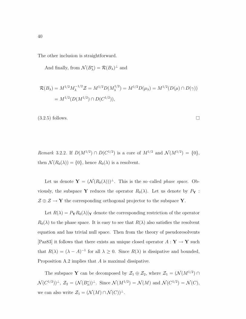
An example is the so–called n–mass oscillator or oscillator ladder given on the
Figure 2.1, where
M = diag(m1, . . . , mn), (2.1.3a)
K =
k0 + k1 −k1
−k1 k1 + k2 −k2
. . . . . . . . .
. . . . . .
−kn−1 kn−1 + kn
, (2.1.3b)
D = de1e∗1, (2.1.3c)
where e1 is the first canonical basis vector.
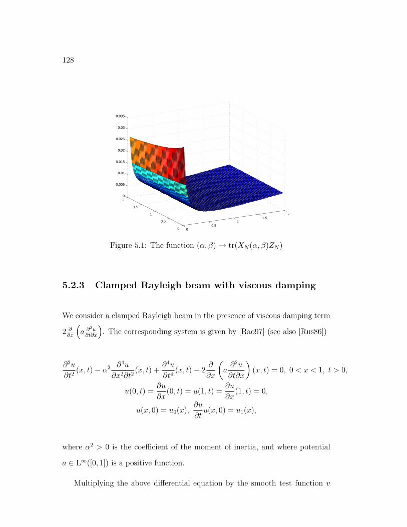
Figure 2.1: The n–mass oscillator with one damper
Here mi > 0 are the masses, ki > 0 the spring constants or stiffnesses and
d > 0 is the damping constant of the damper applied to the mass m1 (Fig. 2.1).
Note that the rank of D is one. Such damping is called one–dimensional.
Obviously, all eigenvalues of (2.1.2) lie in the left complex half–plane. Equa-
tion (2.1.2) can be written as a 2n–dimensional linear eigenvalue problem. This
11
can be done by introducing
y1 = L∗1x, y2 = L∗2x,
where
K = L1L∗1, M = L2L
∗2.
It can be easily seen that (2.1.1) is equivalent to
y = Ay, (2.1.4a)
y(0) = y0, (2.1.4b)
where y = ( y1y2 ), y0 =
(L∗1x0
L∗2x0
), and
A =
(0 L∗1L
−∗2
−L−12 L1 −L−1
2 DL−∗2
), (2.1.5)
with the solution y(t) = eAty0. The eigenvalue problem Ay = λy is obviously
equivalent to (2.1.2).
The basic concept in the vibration theory is its stability. We say that the
matrix A is stable if Reλ < 0 for all λ ∈ σ(A).
In the literature the term ”asymptotically stable” is also used. The famous
result of Lyapunov states that the solution y(t) of the Cauchy problem (2.1.4)
satisfies y(t) → 0 for t → ∞ if and only if A is stable. The following result is
easily proved ([MS85], [Bra98]).
Proposition 2.1.1. The matrix ( 2.1.5) is stable if and only if the form x∗Dx
is non–degenerate on every eigenspace of the matrix M−1K.
This result will be generalized to the infinite–dimensional case in Subsections
3.3.3 and 3.3.4.
12
Our aim is to optimize the vibrational system described by (2.1.1) in the
sense of finding an optimal damping matrix D so as to insure an optimal evanes-
cence.
There exist a number of optimality criteria. The most popular is the spectral
abscissa criterion, which requires that the (penalty) function
D 7→ s(A) := maxk
Reλk
is minimized, where λk are eigenvalues of A (so they are the phase space complex
eigenfrequencies of the system). This criterion concerns the asymptotic behavior
of the system and it is not a priori clear that it will favorably influence the
behavior of the system in finite times, too. More precisely, the asymptotic
formula ‖y(t)‖ ≤ Me−s(A)t holds for all t ≥ 0, where M ≥ 1. There are examples
in which for the minimizing sequence Dn the corresponding coefficients Mn tend
to infinity.
The shortcoming of this criterion is that in the infinite–dimensional case
the quantity s(A) does not describe the asymptotic behavior of the system
accurately (see Remark A.1).
A similar criterion is introduced in [MM91], and is given by the requirement
that the function
D 7→ maxk
Reλk
|λk|is minimized, where λk are as above. This criterion is designed to minimize the
number of oscillations before the system comes to rest.
Both of these criteria are independent of the initial conditions of the system.
Another criterion is given by the requirement for the minimization of the
total energy of the system. The energy of the system (as a sum of kinetic and
13
potential energy) is given by the formula
E(t; x0, x0) (= E(t; y0)) =1
2x(t)∗Mx(t) +
1
2x(t)∗Kx(t).
Note that
y(t)∗y(t) = ‖y(t)‖2 = 2E(t; y0).
In other words, the Euclidian norm of this phase-space representation equals
twice the total energy of the system. The total energy of the system is given by
∞∫
0
E(t; y0)dt. (2.1.6)
Note that this criterion, in the contrast to the criteria mentioned above, does
depend on the initial conditions. The two most popular ways to correct this
defect are:
(i) maximization (2.1.6) over all initial states of unit energy, i.e.
max‖y0‖=1
∞∫
0
E(t; y0)dt, (2.1.7)
(ii) taking the average of (2.1.6) over all initial states of unit energy, i.e.
∫
‖y0‖=1
∞∫
0
E(t; y0)dtdσ, (2.1.8)
where σ is some probability measure on the unit sphere in R2n.
In some simple cases all these criteria lead to the same optimal matrix D,
but in general, they lead to different optimal matrices.
The criterion with the penalty function (2.1.8), introduced in [Ves90], will
be used throughout this thesis. The advantage of this criterion is that we can,
14
by the choice of the appropriate measure σ, implement our knowledge about
the most dangerous input frequencies.
To make this criteria more applicable we proceed as follows.
∞∫
0
E(t; y0)dt =1
2
∞∫
0
y(t; y0)∗y(t; y0)dt =
1
2
∞∫
0
y∗0eA∗teAty0dt
=1
2y∗0Xy0,
where
X =
∞∫
0
eA∗teAtdt. (2.1.9)
The matrix X is obviously positive definite. By the well–known result (see, for
example [LT85]) the matrix X is the solution of the Lyapunov equation
A∗X + XA = −I. (2.1.10)
There exists another integral representation of X [MS85] given by
X =1
2π
∞∫
−∞
(−iη − A∗)−1(iη − A)−1dη. (2.1.11)
This formula will be generalized to the infinite–dimensional case in Section 4.5.
The equation (2.1.10) has the unique solution if and only if A is stable. The
expression (2.1.7) now reads
1
2max‖y0‖=1
y∗0Xy0,
which is simply 12‖X‖, so in this case we minimize the greatest eigenvalue of X.
The expression (2.1.8) now can be written as
1
2
∫
‖y0‖=1
y∗0Xy0dσ.
15
Since with the map
X 7→∫
‖y0‖=1
y∗0Xy0dσ
is given a linear functional on the space of the symmetric matrices, by Riesz
theorem there exists a symmetric matrix Z such that
∫
‖y0‖=1
y∗0Xy0dσ = tr(XZ), for all symmetric X.
Let y ∈ R2n be arbitrary. Set X = yy∗. Then
0 ≤∫
‖y0‖=1
y∗0Xy0dσ = tr(XZ) = tr(yy∗Z) = tr(y∗Zy),
hence Z is always positive semi–definite.
For the measure σ generated by the Lebesgue measure on R2n, we obtain
Z = 12n
I.
Hence the criterion given by the penalty function (2.1.8) can be written as
tr(XZ) → min, (2.1.12)
where X solves (2.1.10), and the matrix Z depends on the measure σ.
Since A is J–symmetric, where J =(
I 00 −I
), it follows that
tr(XZ) = tr(Y ), (2.1.13)
where Y is the solution of another, so–called ”dual Lyapunov equation”
AY + Y A∗ = −Z. (2.1.14)
In some cases, instead of (2.1.9) one can use the expression
∞∫
0
eA∗tQeAtdt,
16
where Q is symmetric (usually positive semi–definite) matrix. We interpret the
matrix Q as a weight function in the total energy integral. In this case the
corresponding Lyapunov equation reads
A∗X + XA = −Q.
A possible choice of the matrix Q is given in Section 4.5.
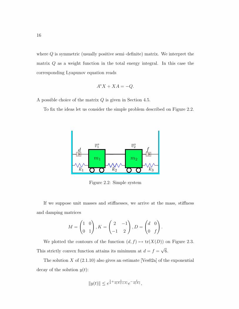
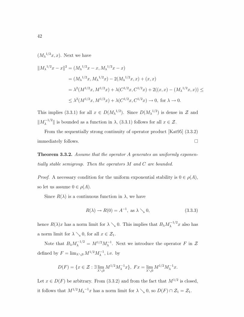
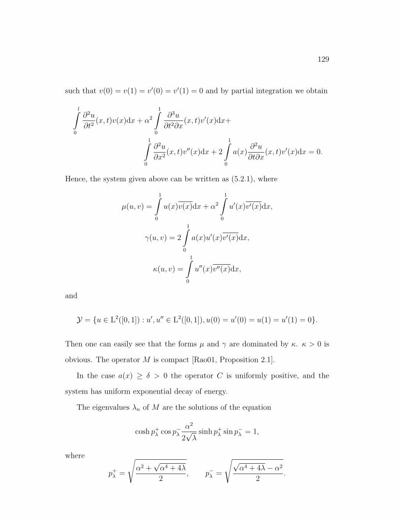
To fix the ideas let us consider the simple problem described on Figure 2.2.
Figure 2.2: Simple system
If we suppose unit masses and stiffnesses, we arrive at the mass, stiffness
and damping matrices
M =
(1 0
0 1
), K =
(2 −1
−1 2
), D =
(d 0
0 f
).
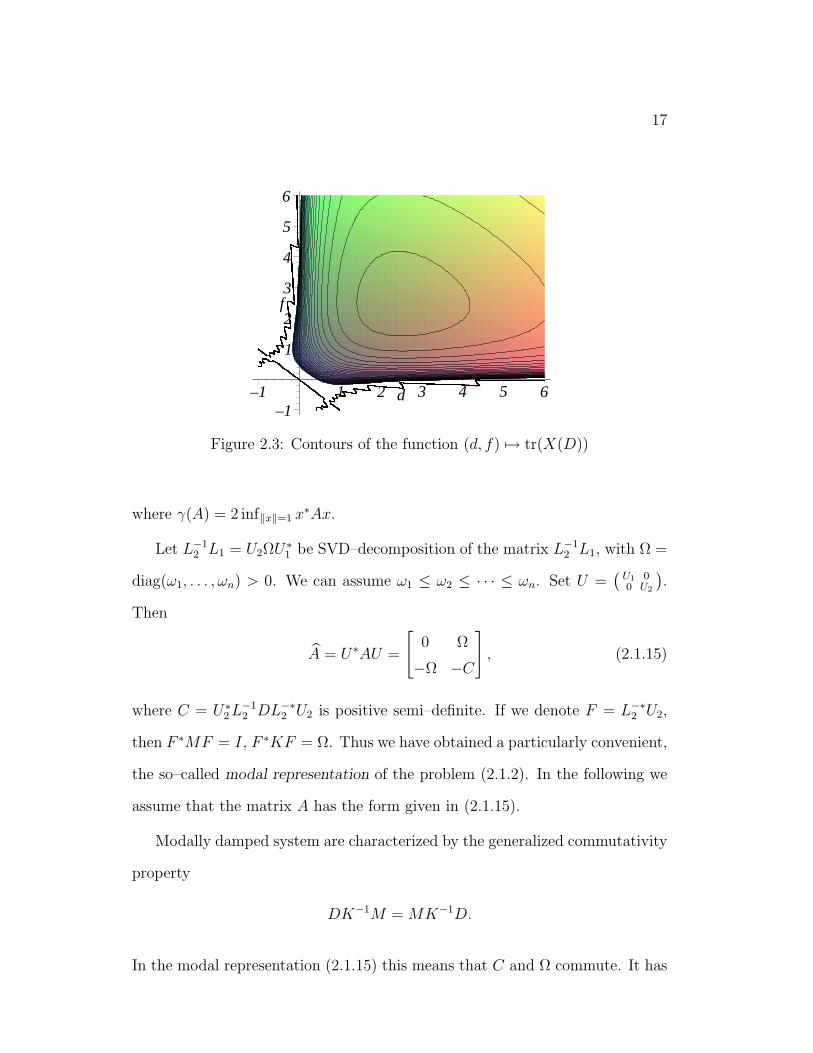
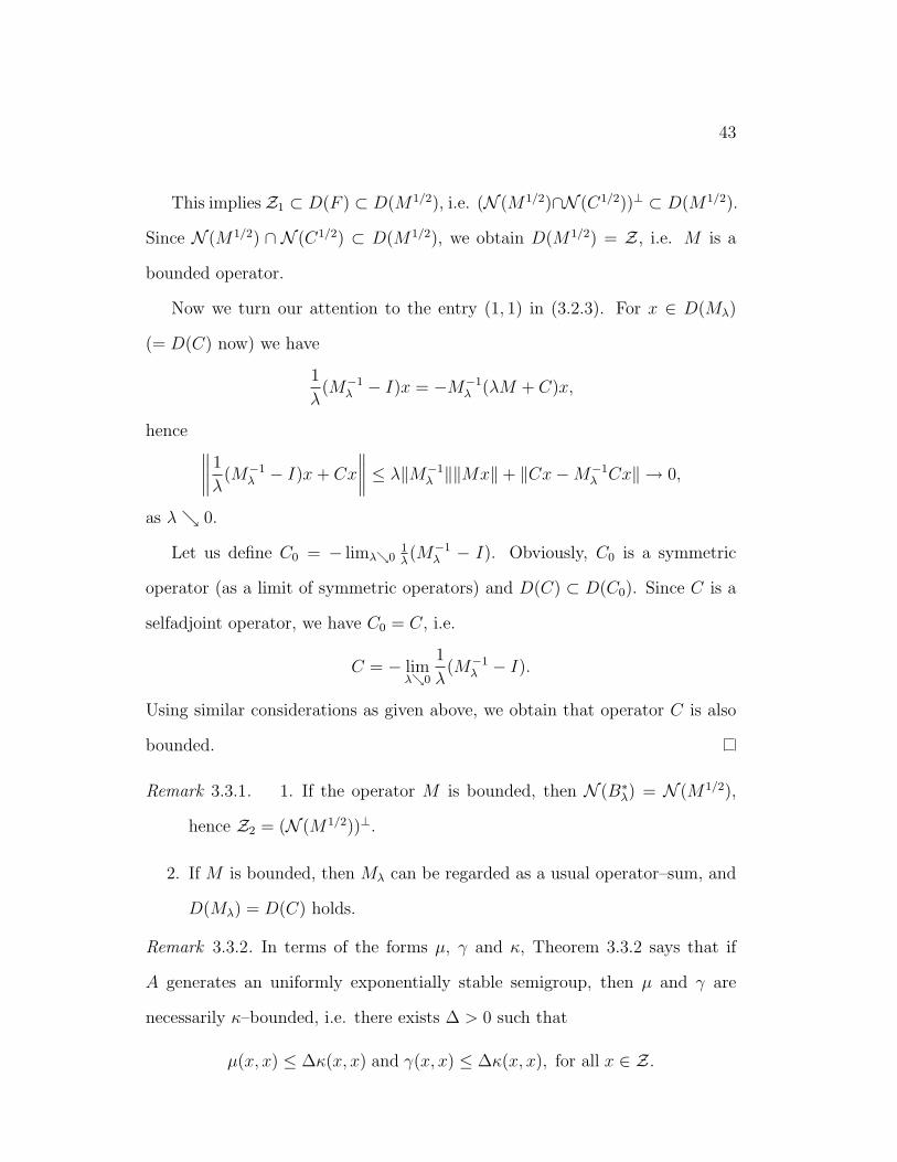
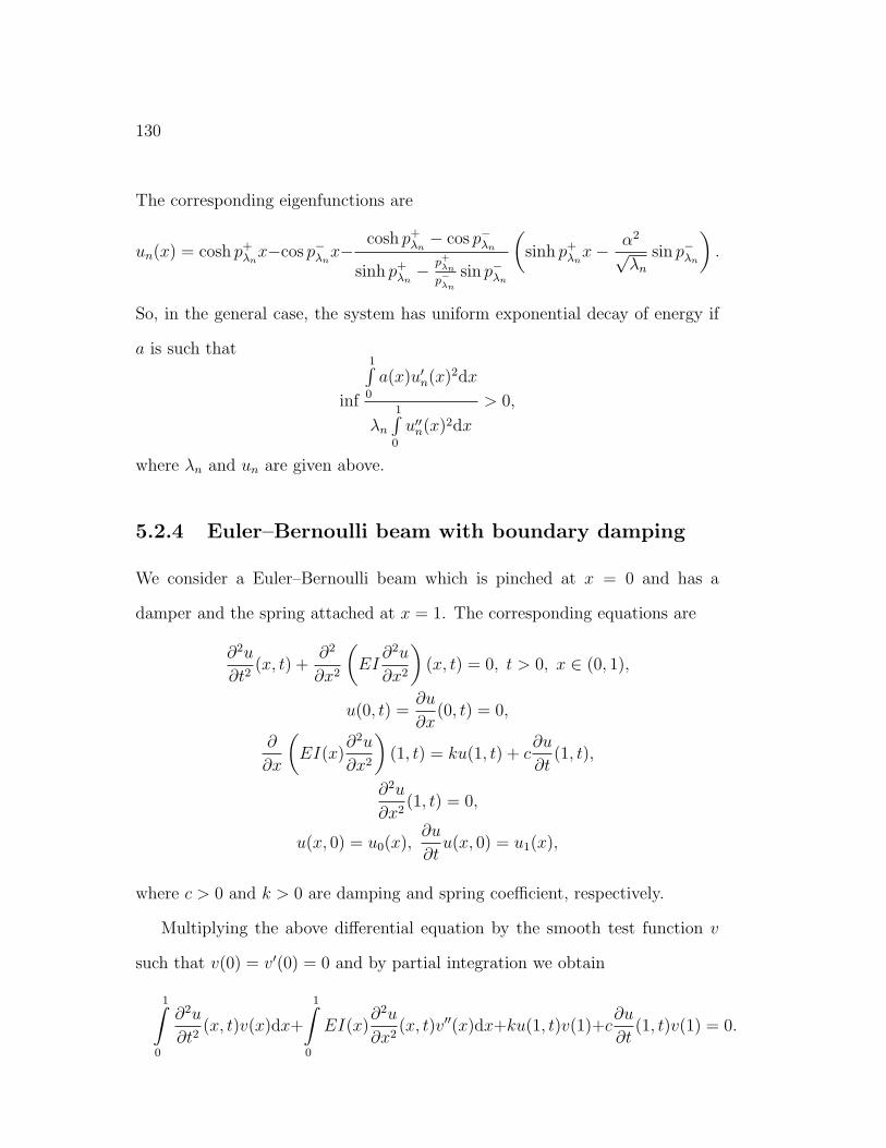
We plotted the contours of the function (d, f) 7→ tr(X(D)) on Figure 2.3.
This strictly convex function attains its minimum at d = f =√
6.
The solution X of (2.1.10) also gives an estimate [Ves02a] of the exponential
decay of the solution y(t):
‖y(t)‖ ≤ e12+ 1
2‖X‖γ(A) e−t
2‖X‖ ,
17
–1
1
2
3
4
5
6
f
–1 1 2 3 4 5 6d
Figure 2.3: Contours of the function (d, f) 7→ tr(X(D))
where γ(A) = 2 inf‖x‖=1 x∗Ax.
Let L−12 L1 = U2ΩU∗
1 be SVD–decomposition of the matrix L−12 L1, with Ω =
diag(ω1, . . . , ωn) > 0. We can assume ω1 ≤ ω2 ≤ · · · ≤ ωn. Set U =(
U1 00 U2
).
Then
A = U∗AU =
[0 Ω
−Ω −C
], (2.1.15)
where C = U∗2 L−1
2 DL−∗2 U2 is positive semi–definite. If we denote F = L−∗2 U2,
then F ∗MF = I, F ∗KF = Ω. Thus we have obtained a particularly convenient,
the so–called modal representation of the problem (2.1.2). In the following we
assume that the matrix A has the form given in (2.1.15).
Modally damped system are characterized by the generalized commutativity
property
DK−1M = MK−1D.
In the modal representation (2.1.15) this means that C and Ω commute. It has
18
been shown in [Cox98b] that
X =
[12CΩ−2 + C−1 1
2Ω−1
12Ω−1 C−1
]. (2.1.16)
Hence, the optimal matrix C, for the criterion with the penalty function (2.1.7)
with Z = I, as well as for the criterion given by (2.1.12), is C = 2Ω. This can
be easily seen in the case when ωi 6= ωj, i 6= j, since then the matrix C must
be diagonal.
This result is generalized to the infinite–dimensional case in Section 4.4. In
the matrix case, this result can be generalized to the case when the matrix
Z has the form Z =( eZ 0
0 eZ ), where Z is diagonal with zeros and ones on the
diagonal.
The case of the friction damping i.e. when D = 2aM , a > 0 was considered
in [Cox98b], where it was shown that the optimal parameter for the criterion
with the penalty function (2.1.7) is a =√
ω1
√√5−12
.
The set of damping matrices over which we optimize the system is deter-
mined by the physical properties of the system. The maximal admissible set
is the set of all symmetric matrices C for which the corresponding matrix A is
stable. Usually, the admissible matrices must be positive semi–definite. The
important case is when the admissible set consists of all positive semi–definite
matrices C for which the corresponding matrix A is stable. For this case Braben-
der [Bra98] (see also [VBD01]) had shown that the following theorem holds.
Theorem 2.1.2. Let the matrix Z be of the form Z =( eZ 0
0 eZ ), where Z = ( Is 0
0 0 ),
1 ≤ s ≤ n. Denote by M the set of all matrices of the form
2
Ωs 0
0 H
, Ωs = diag(ω1, . . . , ωs),
19
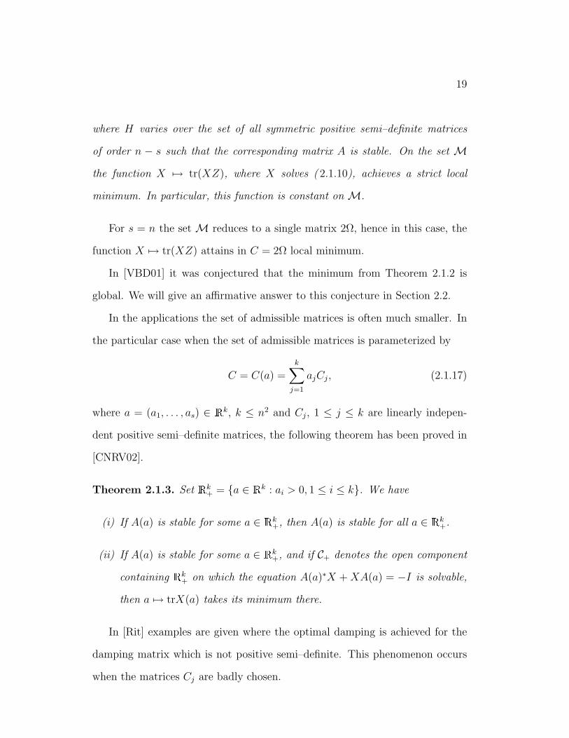
where H varies over the set of all symmetric positive semi–definite matrices
of order n − s such that the corresponding matrix A is stable. On the set Mthe function X 7→ tr(XZ), where X solves ( 2.1.10), achieves a strict local
minimum. In particular, this function is constant on M.
For s = n the set M reduces to a single matrix 2Ω, hence in this case, the
function X 7→ tr(XZ) attains in C = 2Ω local minimum.
In [VBD01] it was conjectured that the minimum from Theorem 2.1.2 is
global. We will give an affirmative answer to this conjecture in Section 2.2.
In the applications the set of admissible matrices is often much smaller. In
the particular case when the set of admissible matrices is parameterized by
C = C(a) =k∑
j=1
ajCj, (2.1.17)
where a = (a1, . . . , as) ∈ Rk, k ≤ n2 and Cj, 1 ≤ j ≤ k are linearly indepen-
dent positive semi–definite matrices, the following theorem has been proved in
[CNRV02].
Theorem 2.1.3. Set Rk+ = a ∈ Rk : ai > 0, 1 ≤ i ≤ k. We have
(i) If A(a) is stable for some a ∈ Rk+, then A(a) is stable for all a ∈ Rk
+.
(ii) If A(a) is stable for some a ∈ Rk+, and if C+ denotes the open component
containing Rk+ on which the equation A(a)∗X + XA(a) = −I is solvable,
then a 7→ trX(a) takes its minimum there.
In [Rit] examples are given where the optimal damping is achieved for the
damping matrix which is not positive semi–definite. This phenomenon occurs
when the matrices Cj are badly chosen.
20
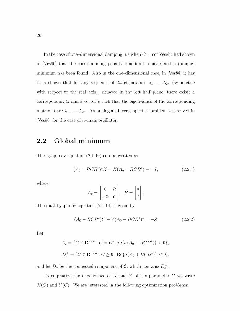
In the case of one–dimensional damping, i.e when C = cc∗ Veselic had shown
in [Ves90] that the corresponding penalty function is convex and a (unique)
minimum has been found. Also in the one–dimensional case, in [Ves88] it has
been shown that for any sequence of 2n eigenvalues λ1, . . . , λ2n (symmetric
with respect to the real axis), situated in the left half–plane, there exists a
corresponding Ω and a vector c such that the eigenvalues of the corresponding
matrix A are λ1, . . . , λ2n. An analogous inverse spectral problem was solved in
[Ves90] for the case of n–mass oscillator.
2.2 Global minimum
The Lyapunov equation (2.1.10) can be written as
(A0 −BCB∗)∗X + X(A0 −BCB∗) = −I, (2.2.1)
where
A0 =
[0 Ω
−Ω 0
], B =
[0
I
].
The dual Lyapunov equation (2.1.14) is given by
(A0 −BCB∗)Y + Y (A0 −BCB∗)∗ = −Z (2.2.2)
Let
Cs = C ∈ Rn×n : C = C∗, Reσ(A0 + BCB∗) < 0,
D+s = C ∈ Rn×n : C ≥ 0, Reσ(A0 + BCB∗) < 0,
and let Ds be the connected component of Cs which contains D+s .
To emphasize the dependence of X and Y of the parameter C we write
X(C) and Y (C). We are interested in the following optimization problems:
21
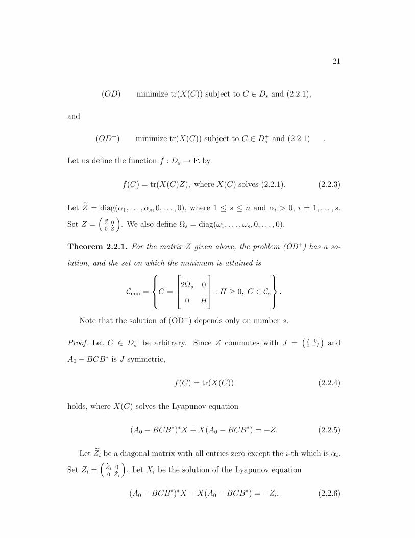
(OD) minimize tr(X(C)) subject to C ∈ Ds and (2.2.1),
and
(OD+) minimize tr(X(C)) subject to C ∈ D+s and (2.2.1) .
Let us define the function f : Ds → R by
f(C) = tr(X(C)Z), where X(C) solves (2.2.1). (2.2.3)
Let Z = diag(α1, . . . , αs, 0, . . . , 0), where 1 ≤ s ≤ n and αi > 0, i = 1, . . . , s.
Set Z =( eZ 0
0 eZ ). We also define Ωs = diag(ω1, . . . , ωs, 0, . . . , 0).
Theorem 2.2.1. For the matrix Z given above, the problem (OD+) has a so-
lution, and the set on which the minimum is attained is
Cmin =
C =
2Ωs 0
0 H
: H ≥ 0, C ∈ Cs
.
Note that the solution of (OD+) depends only on number s.
Proof. Let C ∈ D+s be arbitrary. Since Z commutes with J =
(I 00 −I
)and
A0 −BCB∗ is J-symmetric,
f(C) = tr(X(C)) (2.2.4)
holds, where X(C) solves the Lyapunov equation
(A0 −BCB∗)∗X + X(A0 −BCB∗) = −Z. (2.2.5)
Let Zi be a diagonal matrix with all entries zero except the i-th which is αi.
Set Zi =( eZi 0
0 eZi
). Let Xi be the solution of the Lyapunov equation
(A0 −BCB∗)∗X + X(A0 −BCB∗) = −Zi. (2.2.6)
22
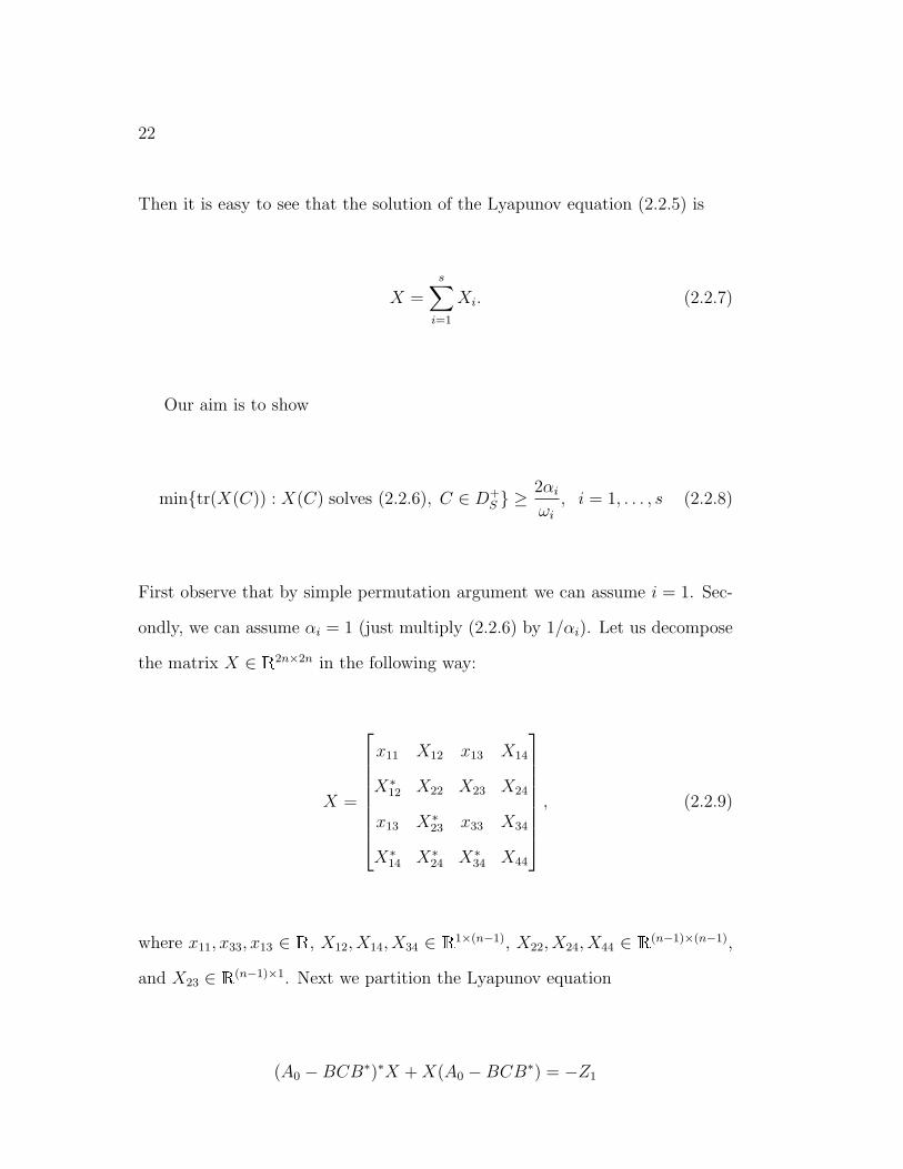
Then it is easy to see that the solution of the Lyapunov equation (2.2.5) is
X =s∑
i=1
Xi. (2.2.7)
Our aim is to show
mintr(X(C)) : X(C) solves (2.2.6), C ∈ D+S ≥
2αi
ωi
, i = 1, . . . , s (2.2.8)
First observe that by simple permutation argument we can assume i = 1. Sec-
ondly, we can assume αi = 1 (just multiply (2.2.6) by 1/αi). Let us decompose
the matrix X ∈ R2n×2n in the following way:
X =
x11 X12 x13 X14
X∗12 X22 X23 X24
x13 X∗23 x33 X34
X∗14 X∗
24 X∗34 X44
, (2.2.9)
where x11, x33, x13 ∈ R, X12, X14, X34 ∈ R1×(n−1), X22, X24, X44 ∈ R(n−1)×(n−1),
and X23 ∈ R(n−1)×1. Next we partition the Lyapunov equation
(A0 −BCB∗)∗X + X(A0 −BCB∗) = −Z1
23
in the same way as we did with X. We obtain
−x13ω1 − ω1x∗13 + 1 = 0 (1,1)
−ω1X∗23 −X14Ωn−1 = 0 (1,2)
−ω1x33 + x11ω1 − x13c11 −X14C∗12 = 0 (1,3)
−ω1X34 + X12Ωn−1 − x13C12 −X14C22 = 0 (1,4)
−Ωn−1X∗24 −X24Ωn−1 = 0 (2,2)
−Ωn−1X∗34 + X∗
12Ω1 −X23c11 −X24C∗12 = 0 (2,3)
−Ωn−1X44 + X22Ωn−1 −X23C12 −X24C22 = 0 (2,4)
ω1x13 − c11x33 − C12XC∗34 + x∗13ω1 − x33c11 −X34C
∗12 + 1 = 0 (3,3)
ω1X14 − c11X34 − C12X44 + X∗23Ωn−1 − x33C12 −X34C22 = 0 (3,4)
Ωn−1X24 − C∗12X34 − C22X44 + X∗
24Ωn−1 −X∗34C12 −X44C22 = 0, (4,4)
where ω1, c11 ∈ R, C12 ∈ R1×(n−1), and C22, Ωn−1 ∈ R(n−1)×(n−1).
From (1,1) we obtain x13 = 12ω1
. One can easily see that c11 = 0 implies
C12 = 0, hence (3,3) reads 2 = 0, a contradiction. Hence, c11 > 0. From (3,3)
we now get
x33 =1−X34C
∗12
c11
. (2.2.10)
The relation (4,4), together with the facts X44 ≥ 0, C22 ≥ 0, implies
tr(C∗12X34 + X∗
34C12) ≤ tr(Ωn−1X24 + X∗24Ωn−1),
and the relation (2,2) implies tr(X24Ωn−1) = 0, hence we obtain
tr(X∗34C12) = tr(X34C
∗12) ≤ 0. (2.2.11)
From the relation (1,3) we obtain
x11 = x33 + x13c11ω−11 + ω−1
1 X14C∗12.
24
From relation (2,4) we obtain
X22 = Ωn−1X44Ω−1n−1 + X23C12Ω
−1n−1 + X24C22Ω
−1n−1,
hence
trX22 = trX44 + tr(X23C12Ω−1n−1) + tr(X24C22Ω
−1n−1).
From the relation (2,2) we obtain
X24 =1
2SΩ−1
n−1,
where S ∈ R(n−1)×(n−1) is a skew–symmetric matrix.
Hence
trX = x11 + trX22 + x33 + trX44
= 2x33 + 2trX44 +c11
2ω21
+1
ω1
X14C∗12 + tr(X23C12Ω
−1n−1) +
1
2tr(SΩ−1
n−1C22Ω−1n−1)
= 2x33 + 2trX44 +c11
2ω21
+1
ω1
X14C∗12 + tr(X23C12Ω
−1n−1).
From the relation (1,2) follows X23 = − 1ω1
Ωn−1X∗14, hence
trX = 2x33 + 2trX44 +c11
2ω21
.
Now (2.2.10) and (2.2.11) imply
trX = 21−X34C
∗12
c11
+c11
2ω21
+ 2trX44 ≥
≥ 2
c11
+c11
2ω21
≥ 2
ω1
.
(2.2.12)
The last inequality follows from the following observation. Let us define the
function g(x) = 2x
+ x2ω2
1. Then the function g attains its unique minimum 2
ω1in
x = 2ω1.
Hence, we have shown (2.2.8). Now (2.2.7) and (2.2.4) imply
tr(X(C)Z) ≥ 2s∑
i=1
αi
ωi
.
25
Since tr(X(2Ω)Z) = 2∑s
i=1αi
ωi, this is indeed the global minimum.
Assume that C ∈ D+s is such that tr(X(C)Z) = 2
∑si=1
αi
ωi. Then (2.2.12)
and (2.2.7) imply trXi = 2ωi
. Observe the matrix X1 which we decompose as in
(2.2.9). Then (2.2.12) implies X44 = 0. Since X1 ≥ 0, it follows X14 = X24 =
X34 = 0. From the relation (1,2) follows immediately X23 = 0. The relation
(1,3) implies x11 = 32
1ω1
, which implies trX22 = 0. Hence X22 = 0. This implies
X12 = 0. Finally, from (1,4) now follows C12 = 0.
By repeating this procedure for i = 2, . . . , s we obtain C ∈ Cmin.
On the other hand, it is easy to see that tr(X(C)Z) = 2∑s
i=1αi
ωi, for all
C ∈ Cmin.
2.3 Numerical aspects
A general algorithm for the optimization of damping does not exist. Available
algorithms optimize only the viscosities of dampers, not their positions, i.e.
they deal with the cases when D is parameterized by some function Rk 3 a 7→C(a) ∈ Rn×n, where k is usually much smaller then n.
Two types of numerical optimization algorithms are currently in use. One
type are the algorithms which rely on the use of Newton–type algorithms for
higher–dimensional (constrained or unconstrained) problems on the function
f defined by (2.2.3) with the use of some Lyapunov solver. The second type
algorithms are ones which bypass the solving of the Lyapunov equation by
explicitly calculating the function f .
The algorithms of the second type, when available, are faster, but harder to
construct. One algorithm of this type is constructed for the case when rank of
26
D is one. In [Ves90] Veselic has given an efficient algorithm which calculates
an optimal ε, where D = εdd∗. Moreover, the optimal viscosity ε is given by a
closed formula.
Recently, a sort of generalization of this algorithm is given in [TV02]. This
algorithm can be used to calculate the optimal viscosity ε if D = εD0.
Note that both of these algorithms only deal with the case when the set of
admissible matrices is parameterized by a real–valued function.
If we want to treat more complex cases, only the algorithms of the first type
are available so far. A major computational effort is spent on the calculation
of the solution of the Lyapunov equation. The standard algorithm is given in
[BS72]. A variant of this general algorithm designed for the Lyapunov equation
is given in [Ham82]. Another algorithm is given in [GNVL79]. There also exist
algorithms based on the iterative methods, see, for example [Saa90], [Wac88]
and [HTP96].
A Newton–type algorithm is developed in [Bra98]. The gradient and the
Hessian of the penalty function can be explicitly calculated.
Chapter 3
Abstract vibrational system
In this chapter we will introduce the notion of an abstract vibrational system
in terms of an abstract second–order differential equation involving quadratic
forms. We will show how we can translate this equation into a linear Cauchy
problem, and we will solve this problem in terms of a semigroup. It turns out
that the norm of the semigroup equals one half of the energy of the solution
of the original differential equation, and that the original differential equation
has a solution if and only if there exists a solution for the Cauchy problem. We
will give necessary and sufficient conditions for uniform exponential stability
of this semigroup in terms of the original coefficients. In generic situation,
uniform exponential stability can be easily checked, if we know the eigenvalues
and eigenvectors of the corresponding undamped system.
3.1 Setting the problem
We start with three symmetric, non–negative sesquilinear forms µ, γ and κ in
a vector space X0 over the complex field. The forms µ, γ and κ correspond to
the mass, damping and stiffness, respectively. We assume that the sesquilinear
27
28
form κ is positive, i.e. κ(x, x) > 0 for all x 6= 0. We also assume that X1 =
D(µ)∩D(γ)∩D(κ) is a non–trivial subspace of X0. We equip the vector space
X1 with the scalar product
(x, y) = κ(x, y), x, y ∈ X1.
This is a natural choice, since it enables us to work in a Hilbert space setting
with the scalar product which corresponds to the energy of the system (see
Example 1.1.1).
Let Z denote the completion of the space (X1, (·, ·)). The norm generated
by this scalar product will be denoted by ‖ · ‖. Obviously, X1 is dense in Z.
For our purposes it will suffice to suppose that the Hilbert space Z is sepa-
rable.
We also assume that µ and γ are closable in Z, and we denote these closures
also by µ and γ. Set X = D(µ) ∩D(γ). The subspace X is obviously dense in
Z. The following definition slightly generalizes the notion of the closability of
forms, introduced in [Kat95] for positive forms.
Definition 3.1.1. Let χ and ξ be symmetric non–negative sesquilinear forms
in a vector space X . We say that χ is ξ–closable if for an arbitrary sequence
(xn), xn ∈ D(ξ) ∩D(χ) with
ξ(xn, xn) → 0, χ(xn − xm, xn − xm) → 0, as n,m →∞,
there exist x ∈ X such that
ξ(x, x) = 0, χ(x− xn, x− xn) → 0.
The following proposition is obvious.
29
Proposition 3.1.1. The sesquilinear forms µ and γ are closable in Z if and
only if µ and γ are κ–closable.
The following formal Cauchy problem
µ(x(t), z) + γ(x(t), z) + (x(t), z) = 0, for all z ∈ Z, t ≥ 0,
x(0) = x0, x(0) = x0,(3.1.1)
where x : [0,∞) → Z, x0, x0 ∈ Z, and µ, γ and κ satisfy the assumptions given
above, is called an abstract vibrational system.
Note that the stiffness form κ is indirectly present in (3.1.1); it defines the
geometry of the underlying space.
We introduce the energy function of the system described by (3.1.1) by
E(t; x0, x0) =1
2µ(x(t), x(t)) +
1
2κ(x(t), x(t)), (3.1.2)
where x(t) is the solution of (3.1.1).
The Cauchy problem (3.1.1) and the energy function (3.1.2) will be central
objects of the investigation in this thesis.
The corresponding undamped system is described by
µ(x(t), z) + (x(t), z) = 0, for all z ∈ Z, t ≥ 0,
x(0) = x0, x(0) = x0.
Example 3.1.1 (Vibrating string). As an illustrative example, throughout this
chapter we will study the following differential equation
∂2
∂t2u(x, t)− ∂2
∂x2u(x, t) = 0, x ∈ [0, π], t ≥ 0, (3.1.3a)
u(0, t) = 0, (3.1.3b)
∂
∂xu(π, t) + ε
∂
∂tu(π, t) = 0, (3.1.3c)
u(x, 0) = u0(x),∂
∂tu(x, 0) = u1(x), (3.1.3d)
30
where ε > 0, and u0, u1 initial data. The equation (3.1.3) describes a homo-
geneous vibrating string with linear boundary damping on its right end. We
multiply equation (3.1.3a) by any continuously differentiable function v with
v(0) = 0, and then partially integrate. Using (3.1.3c) we obtain
π∫
0
∂2
∂t2u(x, t)v(x)dx + ε
∂
∂tu(π, t) +
π∫
0
∂
∂xu(x, t)v′(x)dx = 0.
Thus, we set
µ(u, v) =
π∫
0
u(x)v(x)dx,
γ(u, v) = εu(π)v(π),
κ(u, v) =
π∫
0
u′(x)v′(x)dx,
with X0 := D(µ) = D(γ) = D(κ) = u ∈ C2([0, π]) : u(0) = 0. Hence X1 =
X0. Poincar inequality implies Z = u ∈ L2([0, π]) : u′ ∈ L2([0, π]), u(0) = 0,i.e. Z is the space of all functions from the Sobolev spaceH1([0, π]) which vanish
in π. Also, the scalar product generated by κ and standard scalar product in
H1([0, π]) are equivalent.
Next we will show that µ and γ are κ–closable. Indeed, κ(un, un) → 0
implies u′n → 0 in L2–norm, and µ(un − um, un − um) → 0 for n,m → ∞implies the existence of u ∈ L2([0, π]) such that un → u in L2–norm. From
Poincar inequality now follows u = 0, hence µ is κ–closable. From γ(un −um, un − um) → 0 and Poincar inequality follows |un(π)|2 ≤ ‖u′n‖2
L2 → 0, so γ
is also κ–closable. Obviously, the closures of µ and γ (which we again denote
31
by µ and γ) are defined on all Z. Hence, the system (3.1.3) can be written as
µ(u, v) + γ(u, v) + (u, v) = 0, for all v ∈ Z,
u(0) = u0, u(0) = u1, u0, u1 ∈ Z.
(3.1.4)
For (3.1.1), the formal substitution x(t) = eλty leads to
λ2µ(y, z) + λγ(y, z) + (y, z) = 0.
The form µλ = λ2µ + λγ + I is densely defined (with the domain X ) closed
(as a sum of closed symmetric forms) positive form for all λ > 0.
For λ ≥ 0, the second representation theorem [Kat95, pp. 331] implies the
existence of selfadjoint non–negative operators M and C such that
D(M1/2) = D(µ), µ(x, y) = (M1/2x, M1/2y), x, y ∈ D(µ),
D(C1/2) = D(γ), γ(x, y) = (C1/2x, C1/2y), x, y ∈ D(γ),
and a selfadjoint positive operator Mλ such that
D(Mλ1/2) = D(µλ), µλ(x, y) = (Mλ
1/2x,Mλ1/2y), x, y ∈ D(µλ).
Obviously,
D(Mλ1/2) ⊂ D(M1/2) and D(Mλ
1/2) ⊂ D(C1/2) for all λ > 0,
and
µλ(x, x) ≥ ‖x‖2 for all λ ≥ 0. (3.1.5)
We write
Mλ = λ2M + λC + I,
32
in the form–sum sense. From (3.1.5) follows that M−1/2λ exists and is everywhere
defined bounded operator, and ‖M−1/2λ ‖ ≤ 1 holds for all λ ≥ 0. This obviously
implies ‖M−1λ ‖ ≤ 1 for all λ ≥ 0. Note also that M0 = I.
Now (3.1.1) can be written as
(M1/2x(t),M1/2z) + (M1/2x(t),M1/2z) + (x(t), z) = 0, for all z ∈ Z, t ≥ 0,
x(0) = x0, x(0) = x0,
(3.1.6)
and the energy function (3.1.2) can be written as
E(t; x0, x0) =1
2‖M1/2x(t)‖2 +
1
2‖x(t)‖2 (3.1.7)
Example 3.1.2 (Continuation of Example 3.1.1). A straightforward computation
gives
(Mu)(x) =
π∫
0
G(x, ξ)u(ξ)dξ,
(Cu)(x) = εu(π)x,
where G is the Green function of the corresponding undamped system given by
G(x, ξ) =
x, x ≤ ξ,
ξ, x ≥ ξ
.
Both operators are everywhere defined, and M is compact. Obviously,
N (M) = 0. The operator C has one–dimensional range spanned by the
identity function. Observe that M1/2 and C1/2 cannot be written in a closed
form.
The energy function of the system (3.1.3) is given by
E(t; u0, u1) =1
2
π∫
0
(|x(t)|2 + |x(t)|2) dx. (3.1.8)
33
3.2 The pseudoresolvent
From D(Mλ1/2) ⊂ D(M1/2) follows that M1/2M−1
λ is a closed operator defined
on all Z, hence by
Bλ = M1/2M−1/2λ
is given a bounded operator in Z, for all λ > 0.
The adjoint B∗λ of Bλ is then also bounded, and it is the closure of the
densely defined operator M−1/2λ M1/2, i.e.
B∗λ = M
−1/2λ M1/2.
To prove this, first note that D(M−1/2λ M1/2) = D(M1/2). From [Wei76, Satz
4.19] we have
(M−1/2λ M1/2)∗ = M1/2M
−1/2λ = Bλ.
Hence from [Wei76, Satz 4.13] follows
M−1/2λ M1/2 = (M
−1/2λ M1/2)∗∗ = B∗
λ.
For λ > 0 we have
µ ≤ µ +1
λγ +
1
λ2I =
µλ
λ2,
hence
‖Bλx‖2 = (M1/2M−1/2λ x,M1/2M
−1/2λ x) = µ(M
−1/2λ x) ≤
≤ µλ(M−1/2λ x)
λ2=‖x‖2
λ2.
This implies
‖Bλ‖ ≤ 1
λ, ‖B∗
λ‖ ≤1
λ, for all λ > 0.
34
In the finite–dimensional case the corresponding equation (3.1.1) reads
Mx + Cx + x = 0. (3.2.1)
Substituting y1 = x, y2 = M1/2x, it is easy to see that (3.2.1) is equivalent with
the matrix differential equation
y = Afy,
where y = ( y1y2 ), and
Af =
[0 M−1/2
−M−1/2 −M−1/2CM−1/2
].
By a straightforward computation one can obtain
(Af − λ)−1 =
[1λ(M−1
λ − I) −M−1λ M1/2
M1/2M−1λ −λM1/2M−1
λ M1/2,
], (3.2.2)
which is a well-known formula.
In the general case the operator given by (3.2.2) may not exist. Hence, to
bypass this, we define a family of bounded operators in Z ⊕Z, which, in some
sense, generalizes (3.2.2), by
R0(λ) =
[1λMλ
−1 − 1λ−Mλ
−1/2B∗λ
BλMλ−1/2 −λBλB
∗λ
], λ > 0. (3.2.3)
In the matrix case, it is easy to see that (3.2.3) is equivalent with (3.2.2).
Next we will show that R0(λ) is a pseudoresolvent.
Lemma 3.2.1. For all λ, ν > 0, and all x, y ∈ Z we have
(λMλ−1x−νM−1
ν x, y) = (λ−ν)[−λν(BνM
−1/2ν x,BλMλ
−1/2y) + (M−1ν x,Mλ
−1y)]
35
Proof. We have
µλ(M−1ν x,M−1
λ y) = (Mλ1/2M−1
ν x,Mλ−1/2y) = (M−1
ν x, y),
µν(M−1ν x,M−1
λ y) = (M−1λ x, y).
Hence,
(λM−1λ x− νM−1
ν x, y) = λ(M−1λ x, y)− ν(M−1
ν x, y)
= λµν(M−1ν x,M−1
λ y)− νµλ(M−1ν x, M−1
λ y)
= (λ− µ)[−λνµ(M−1
ν x,M−1λ y) + (M−1
ν x,M−1λ y)
].
Now, from
µ(M−1ν x,M−1
λ y) = (M1/2M−1ν x,M1/2M−1
λ y) = (BνM−1/2ν x,BλMλ
−1/2y),
our claim follows.
Proposition 3.2.2. The operator family R0(λ) : λ > 0 satisfies the resolvent
equation
R0(λ)−R0(ν) = (λ− ν)R0(λ)R0(ν), (3.2.4)
i.e. R0(λ) is a pseudoresolvent.
Proof. Let us denote the operator matrix on the left hand side and the right
hand side of (3.2.4) by
b11 b12
b21 b22
and
a11 a12
a21 a22,
,
36
respectively. From the straightforward computation we get
a11 =λ− ν
λν(M−1
λ M−1ν −M−1
λ −M−1ν + I)− (λ− ν)(Mλ
−1/2B∗λBνM
−1/2ν ),
a12 =λ− ν
ν(BλMλ
−1/2M−1ν −BλMλ
−1/2)− λ(λ− ν)BλB∗λBνM
−1/2ν ,
a21 = −λ− ν
λM−1
λ M−1/2ν B∗
ν +λ− ν
λM−1/2
ν B∗ν + ν(λ− ν)Mλ
−1/2B∗λBνB
∗ν ,
a22 = (λ− ν)(−BλMλ−1/2M−1/2
ν B∗ν + λνBλB
∗λBνB
∗ν).
Let x, y ∈ D(M1/2) be arbitrary, and let us denote u = M1/2x, v = M1/2y.
Then B∗νx = M
−1/2ν u and B∗
λy = Mλ−1/2v.
First we show that a22 = b22. Let us now calculate (a22x, y). Using Lemma
3.2.1 we obtain
(a22x, y) = (λ− ν)[−(BλMλ
−1/2M−1/2ν B∗
νx, y) + λν(BλB∗λBνB
∗νx, y)
]
= (λ− ν)[−(Mλ
−1/2M−1ν u,Mλ
−1/2v) + λν(B∗λBνM
−1/2ν u,Mλ
−1/2v)]
= (λ− ν)[λν(BνM
−1/2ν u, BλMλ
−1/2v)− (M−1ν u,M−1
λ v)]
= −λ(M−1λ u, v) + ν(M−1
ν u, v)
= −λ(M1/2M−1λ M1/2x, y) + ν(M1/2M−1
ν M1/2x, y)
= −λ(BλB∗λx, y) + ν(BνB
∗νx, y) = (b22x, y).
Since D(M1/2) is dense in Z, and operators a22 and b22 are bounded we have
(a22x, y) = (b22x, y) for all x, y ∈ Z, hence a22 = b22.
37
Next we show a12 = b12. Again, using Lemma 3.2.1 we obtain
(a12x, y) = −λ− ν
λ
[(M−1
λ M−1ν u, y)− (M−1
ν u, y)− λν(Mλ−1/2B∗
λBνM−1/2ν u, y)
]
= −λ− ν
λ
[(M−1
ν u,M−1λ y)− (M−1
ν u, y)− λν(BνM−1/2ν u,BλMλ
−1/2y)]
= −1
λ(λM−1
λ u− νM−1ν u, y) +
λ− ν
λ(M−1
ν u, y)
= −1
λ
[λ(M−1
λ u, y)− ν(M−1ν u, y)− λ(M − ν−1u, y) + ν(M − ν−1u, y)
]
= (M−1ν u, y)− (M−1
λ u, y) = (M−1ν uB∗
νx, y)− (M−1λ uB∗
λx, y) = (b12x, y),
hence again a12 = b12.
Similarly, one can also prove that a21 = b21.
The term (a11x, y) can be written as
(a11x, y) = −1
λ+
1
ν+
+λ− ν
λν
[(M−1
ν x,M−1λ y)− (M−1
λ x, y)− (M−1ν x, y)− λν(BνM
−1/2ν x,BλM
−1/2λ y)
],
and since
(b11x, y) = −1
λ+
1
ν+
1
λ(M−1
λ x, y)− 1
ν(M−1
ν x, y),
to see that (a11x, y) equals (b11x, y), we have to show that
λ− ν
λν
[(M−1
ν x,M−1λ y)− (M−1
λ x, y)− (M−1ν x, y)− λν(BνM
−1/2ν x,BλM
−1/2λ y)
]
=1
λ(M−1
λ x, y)− 1
ν(M−1
ν x, y).
But this easily follows from Lemma 3.2.1.
Let us define
J =
[I 0
0 −I
], in Z ⊕ Z.
Proposition 3.2.3. The operators R0(λ) and R0(λ)∗ are dissipative and J–
selfadjoint, for all λ > 0.
38
Proof. Let u = ( xy ) ∈ Z ⊕ Z. Then
(R0(λ) ( xy ) , ( x
y )) = −1
λ‖x‖2 +
1
λ(M−1
λ x, x) + 2iIm(BλM−1/2λ x, y)− ‖B∗
λy‖2.
Now,
Re (R0(λ) ( xy ) , ( x
y )) = −1
λ‖x‖2 +
1
λ(M−1
λ x, x)− ‖B∗λy‖2 ≤
≤ −1
λ‖x‖2 +
1
λ‖x‖2 − ‖B∗
λy‖2 ≤ 0,
hence R0(λ) is dissipative.
On the other hand
Re(R0(λ)∗x, x) = Re(x,R0(λ)x) = Re(R0(λ)x, x) = Re(R0(λ)x, x) ≤ 0.
The fact that R0(λ) is J–selfadjoint is obvious.
Proposition 3.2.4. The null–space of the operator R0(λ) is given by
N (R0(λ)) =u ∈ Z ⊕ Z : u = ( x
y ) , x ∈ N (M1/2) ∩N (C1/2), y ∈ N (B∗λ)
,
where
N (B∗λ) =
(M1/2(D(M1/2) ∩D(C1/2))
)⊥. (3.2.5)
Remark 3.2.1. 1. The set N (R0(λ)) is independent of λ, which is a property
shared by all pseudoresolvents, see for example [Paz83].
2. If D(M1/2) ∩ D(C1/2) is a core of the operator M1/2 then N (B∗λ) =
N (M1/2), but in general we have only N (B∗λ) ⊃ N (M1/2). This is a
mild regularity condition which will be fulfilled in most applications.
Proof of Proposition 3.2.4. From the equation R0(λ)u = 0, where u = ( xy ), it
follows
1
λM−1
λ x− 1
λx−M
−1/2λ B∗
λy = 0,
BλM−1/2λ x− λBλB
∗λy = 0.
39
Multiplying the first equation by λx, and second by λy and then conjugate, we
get
(M−1λ x, x)− (x, x)− λ(M
−1/2λ B∗
λy, x) = 0, (3.2.6)
λ(M−1/2λ B∗
λy, x)− λ2(BλB∗λy, y) = 0. (3.2.7)
Adding (3.2.6) and (3.2.7) we obtain
(M−1λ x, x)− (x, x)− λ2(BλB
∗λy, y) = 0,
which implies
(M−1λ x, x)− (x, x) = λ2(BλB
∗λy, y) ≥ 0. (3.2.8)
Since ‖M−1λ ‖ ≤ 1, it follows (x, x) ≥ (M−1
λ x, x) ≥ (x, x), hence
(M−1λ x, x) = (x, x), (3.2.9)
and since N (R0(λ)) is independent of the choice of λ, this equation holds for
all λ > 0. Also, from (3.2.8) follows B∗λy = 0.
Let us denote z = M−1/2λ x. Then (3.2.9) reads (z, z) = (Mλ
1/2z,Mλ1/2z).
Hence,
(z, z) = λ2(M1/2z,M1/2z) + λ(C1/2z, C1/2z) + (z, z).
This implies
λ2(M1/2z, M1/2z) + λ(C1/2z, C1/2z) = 0, for all λ > 0,
so we obtain M1/2z = C1/2z = 0. Hence, (λ2M1/2 + λC1/2)z = 0, for all λ > 0,
which implies Mλ1/2z = z. This implies M
−1/2λ x = x, hence λ2M1/2x+λC1/2x =
0 for all λ > 0, so we finally obtain M1/2x = C1/2x = 0. Hence we have shown
N (R0(λ)) ⊂ u ∈ Z ⊕ Z : u = ( x
y ) , x ∈ N (M1/2) ∩N (C1/2), y ∈ N (B∗λ)
.
40
The other inclusion is straightforward.
And finally, from N (B∗λ) = R(Bλ)
⊥ and
R(Bλ) = M1/2M−1/2λ Z = M1/2D(M
1/2λ ) = M1/2D(µλ) = M1/2(D(µ) ∩D(γ))
= M1/2(D(M1/2) ∩D(C1/2)),
(3.2.5) follows.
Remark 3.2.2. If D(M1/2) ∩ D(C1/2) is a core of M1/2 and N (M1/2) = 0,then N (R0(λ)) = 0, hence R0(λ) is a resolvent.
Let us denote Y = (N (R0(λ)))⊥. This is the so–called phase space. Ob-
viously, the subspace Y reduces the operator R0(λ). Let us denote by PY :
Z ⊕ Z → Y the corresponding orthogonal projector to the subspace Y.
Let R(λ) = PYR0(λ)|Y denote the corresponding restriction of the operator
R0(λ) to the phase space. It is easy to see that R(λ) also satisfies the resolvent
equation and has trivial null space. Then from the theory of pseudoresolvents
[Paz83] it follows that there exists an unique closed operator A : Y → Y such
that R(λ) = (λ − A)−1 for all λ ≥ 0. Since R(λ) is dissipative and bounded,
Proposition A.2 implies that A is maximal dissipative.
The subspace Y can be decomposed by Z1 ⊕ Z2, where Z1 = (N (M1/2) ∩N (C1/2))⊥, Z2 = (N (B∗
λ))⊥. Since N (M1/2) = N (M) and N (C1/2) = N (C),
we can also write Z1 = (N (M) ∩N (C))⊥.
41
3.3 Uniform exponential stability
3.3.1 The operator A−1
Since A is maximal dissipative, the Lumer–Phillips theorem A.3 implies that A
generates a contractive strongly continuous semigroup.
Our next aim is to explore properties of the semigroup generated by the
operator A and to explain the connection of this semigroup with our quadratic
problem. We also find necessary and sufficient conditions which ensure that our
semigroup is uniformly exponentially stable.
To achieve this goal, we have to find some suitable representation of A in
the space Z1 ⊕ Z2. Unfortunately, in general, the operator A does not have
block–matrix representation in the product space Z1 ⊕Z2, but its inverse has.
First we will show that a necessary condition for the uniform exponential
stability of the semigroup generated by A is that M and C are bounded.
We will need the following lemma.
Lemma 3.3.1. For an arbitrary x ∈ Z and λ > 0 we have
limλ→0
M−1/2λ x− x → 0, (3.3.1)
limλ→0
M−1λ x− x → 0. (3.3.2)
Proof. Let x ∈ D(Mλ1/2) be arbitrary. We have
‖M−1/2λ x− x‖ = ‖M−1
λ Mλ1/2x−Mλ
1/2x + Mλ1/2x− x‖ ≤
≤ (‖M−1λ ‖+ 1)‖Mλ
1/2x− x‖ ≤ 2‖Mλ1/2x− x‖.
Now first observe that ‖x‖ ≤ ‖Mλx‖ implies (using Heinz inequality) (x, x) ≤
42
(Mλ1/2x, x). Next we have
‖Mλ1/2x− x‖2 = (Mλ
1/2x− x,Mλ1/2x− x)
= (Mλ1/2x,Mλ
1/2x)− 2(Mλ1/2x, x) + (x, x)
= λ2(M1/2x,M1/2x) + λ(C1/2x,C1/2x) + 2((x, x)− (Mλ1/2x, x)) ≤
≤ λ2(M1/2x,M1/2x) + λ(C1/2x,C1/2x) → 0, for λ → 0.
This implies (3.3.1) for all x ∈ D(Mλ1/2). Since D(Mλ
1/2) is dense in Z and
‖M−1/2λ ‖ is bounded as a function in λ, (3.3.1) follows for all x ∈ Z.
From the sequentially strong continuity of operator product [Kat95] (3.3.2)
immediately follows.
Theorem 3.3.2. Assume that the operator A generates an uniformly exponen-
tially stable semigroup. Then the operators M and C are bounded.
Proof. A necessary condition for the uniform exponential stability is 0 ∈ ρ(A),
so let us assume 0 ∈ ρ(A).
Since R(λ) is a continuous function in λ, we have
R(λ) → R(0) = A−1, as λ 0, (3.3.3)
hence R(λ)x has a norm limit for λ 0. This implies that BλM−1/2λ x also has
a norm limit for λ 0, for all x ∈ Z1.
Note that BλM−1/2λ = M1/2M−1
λ . Next we introduce the operator F in Zdefined by F = limλ0 M1/2M−1
λ , i.e. by
D(F ) = x ∈ Z : ∃ limλ0
M1/2M−1λ x, Fx = lim
λ0M1/2M−1
λ x.
Let x ∈ D(F ) be arbitrary. From (3.3.2) and from the fact that M1/2 is closed,
it follows that M1/2Mλ−1x has a norm limit for λ 0, so D(F ) ∩ Z1 = Z1.
43
This implies Z1 ⊂ D(F ) ⊂ D(M1/2), i.e. (N (M1/2)∩N (C1/2))⊥ ⊂ D(M1/2).
Since N (M1/2) ∩ N (C1/2) ⊂ D(M1/2), we obtain D(M1/2) = Z, i.e. M is a
bounded operator.
Now we turn our attention to the entry (1, 1) in (3.2.3). For x ∈ D(Mλ)
(= D(C) now) we have
1
λ(M−1
λ − I)x = −M−1λ (λM + C)x,
hence∥∥∥∥
1
λ(M−1
λ − I)x + Cx
∥∥∥∥ ≤ λ‖M−1λ ‖‖Mx‖+ ‖Cx−M−1
λ Cx‖ → 0,
as λ 0.
Let us define C0 = − limλ01λ(M−1
λ − I). Obviously, C0 is a symmetric
operator (as a limit of symmetric operators) and D(C) ⊂ D(C0). Since C is a
selfadjoint operator, we have C0 = C, i.e.
C = − limλ0
1
λ(M−1
λ − I).
Using similar considerations as given above, we obtain that operator C is also
bounded.
Remark 3.3.1. 1. If the operator M is bounded, then N (B∗λ) = N (M1/2),
hence Z2 = (N (M1/2))⊥.
2. If M is bounded, then Mλ can be regarded as a usual operator–sum, and
D(Mλ) = D(C) holds.
Remark 3.3.2. In terms of the forms µ, γ and κ, Theorem 3.3.2 says that if
A generates an uniformly exponentially stable semigroup, then µ and γ are
necessarily κ–bounded, i.e. there exists ∆ > 0 such that
µ(x, x) ≤ ∆κ(x, x) and γ(x, x) ≤ ∆κ(x, x), for all x ∈ Z.
44
From now on, in the rest of thesis, we assume the following:
The operators M and C are bounded.
Note that now M−1/2λ B∗
λ = M−1λ M1/2.
Using previous considerations and the fact that R(C) ⊂ Z1 and R(M1/2) ⊂Z1, we obtain
A−1 =
[−C|Z1 −M1/2|Z2
M1/2|Z1 0
].
Note that the phase space now becomes Y = Z1⊕Z2 = (N (M1/2)∩N (C1/2))⊥⊕(N (M1/2))⊥. The operators C|Z1 and M1/2|Z1 are obviously bounded symmetric
operators in the space Z1, hence they are selfadjoint.
To avoid technicalities and simplify the proofs, we assume N (M1/2) ⊂N (C1/2), i.e. there is no damping on the positions where mass vanishes. All the
results of this thesis remain valid also in the case when N (M1/2) * N (C1/2).
This assumption implies Y := Z1 = Z2, so now Y = Y ⊕ Y . Also, from
now on let C denote the operator C : Y → Y , and let M denote the operator
M : Y → Y . Letters M and C will denote operators in the spaces Z or Ydepending on the context.
Hence we can write
A−1 =
[−C −M1/2
M1/2 0
].
From
A−1
[x
M1/2y
]=
[−Cx−M1/2y
M1/2x
]
follows that D(A) = R(A−1) = (R(C) +R(M1/2))⊕R(M1/2), hence the oper-
ator A is not bounded in general.
45
Remark 3.3.3. The operator A cannot, in general, be written in the block-matrix
form in Y ⊕ Y . Indeed, let us suppose that the operator A can be written in
the block–matrix form. Then we obtain R(C) ⊂ R(M1/2), and this does not
hold in general, as we can see from the following example.
Example 3.3.1 (Continuation of Example 3.1.2). As we have seen, M and C are
bounded, hence satisfy our assumption. Since N (M) = 0 we have Y = Z.
Next we show that A cannot be written in block–matrix form. To see this, it
is sufficient to show that the identity function is not in R(M1/2). First observe
that
(M−1/2u,M−1/2v) =
π∫
0
u′′(x)v′′(x)dx.
Let us assume that u(x) = x is in R(M1/2). Then there exists v ∈ Y such that
u = M1/2v. Hence
(v, v) = (M−1/2u,M−1/2u) =
π∫
0
|u′′(x)|2dx = 0,
a contradiction.
Observe also that R(C) +R(M1/2) 6= Y , hence A is not bounded.
Next we want to compute the resolvent of the operator A. Since A is maxi-
mal dissipative, the spectrum of A is contained in the left complex half–plane.
Our candidate for the resolvent of A is R(λ). Obviously, R(λ) is resolvent of A
for all λ ≥ 0. Next we show that R(λ) can be written as a block–matrix in Y Yby
(A−λ)−1 ( xy ) = R(λ) ( x
y ) =
[1λ(M−1
λ − I) −M−1λ M1/2
M1/2M−1λ −λM1/2M−1
λ M1/2
] [x
y
], for all x, y ∈ Y ,
(3.3.4)
46
i.e.
(M−1λ − I)x ∈ Y , M−1
λ M1/2x ∈ Y ,
M1/2M−1λ x ∈ Y , M1/2M−1
λ M1/2x ∈ Y ,
holds for all x ∈ Y and all λ ≥ 0. The last two assertions are trivial. To prove
the first one, decompose (M−1λ −I)x as (M−1
λ −I)x = y1+y2, where y1 ∈ N (M),
y2 ∈ Y . Then −λ2Mx−λCx = y1 +Mλy2, hence y1 ∈ Y , so y1 = 0. The second
assertion can be proved similarly. It is evident that R(λ) is well defined and
bounded operator for all λ such that 0 ∈ ρ(Mλ).
Let λ ∈ ρ(A) be such that 0 ∈ ρ(Mλ). Then it follows (I−λA−1)R(λ) = A−1,
hence R(λ)x ∈ D(A), for all x ∈ Y , which implies (A − λ)R(λ)x = x for all
x ∈ Y .
Similarly one can also prove R(λ)A−1 = A−1R(λ), hence R(λ)(I − λA−1) =
A−1. This implies R(λ)(A− λ)x = x, for all x ∈ D(A).
3.3.2 The spectrum of the operator A
Our aim in this section is to establish the correspondence between various types
of spectra of the operator A and the operator function λ 7→ Mλ.
Let us denote by ρ, σ, σp, σap and σr the resolvent set, spectrum, point spec-
trum, approximate point spectrum and residual spectrum of the operator func-
tion λ 7→ Mλ = λ2M + λC + I in the space Z, respectively. The point λ is in
the point spectrum of the operator function L if zero is in the point spectrum
of the operator L(λ), and analogous definitions hold for the other parts of the
spectrum. Note that now Mλ can be viewed as an operator sum.
47
Theorem 3.3.3. The following holds:
ρ = ρ(A), σ = σ(A), σp = σp(A), σap = σap(A) and σr = σr(A).
Proof. Since 0 ∈ ρ(A) and M0 = I, we can assume λ 6= 0.
First we consider the point spectrum. Let λ ∈ σp, λ 6= 0 be arbitrary. Then
there exists x 6= 0 such that λ2Mx+λCx+x = 0, hence x = −λ2Mx−λCx ∈ Y .
Let us denote y = λM1/2x ∈ Y . Then ( xy ) ∈ Y. From
A−1
x
y
=
−Cx− λMx
M1/2x
=
1
λ
x
y
follows 1λ∈ σp(A
−1), hence λ ∈ σp(A).
On the other hand, let λ ∈ σp(A), λ 6= 0 be arbitrary. Then there exists
( xy ) 6= 0 such that
−C −M1/2
M1/2 0
x
y
=
1
λ
x
y
,
hence
−Cx−M1/2y =1
λx,
M1/2x =1
λy.
From this one can easily obtain λ2Mx + λCx + x = 0. We can assume x 6= 0,
since x = 0 implies y = 0, so λ ∈ σp holds.
Let now λ ∈ σap, λ 6= 0 be arbitrary. Then there exists a sequence (xn),
‖xn‖ = 1 such that Mλxn → 0 as n →∞. We decompose xn as xn = x1n + x2
n,
with x1n ∈ Y , x2
n ∈ N (M) = N (M) ∩N (C). Then
Mλxn = λ2Mx1n + λCx1
n + x1n + x2
n → 0,
48
which implies λ2Mx1n + λCx1
n + x1n → 0 and x2
n → 0, hence we can assume
xn ∈ Y . Let us define yn = λM1/2xn. We have
(A−1−1
λ)
xn
yn
=
−Cxn − 1
λxn −M1/2yn
M1/2xn − 1λyn
=
1
λ
−λ2Mxn − λCxn − xn
0
→ 0,
as n →∞. Since ‖( xnyn )‖ ≥ 1, we have λ ∈ σap(A).
On the other hand, let be λ ∈ σap(A), λ 6= 0 be arbitrary. Then there exists
a sequence ( xnyn ) ∈ Y, ‖xn‖2 + ‖yn‖2 = 1 such that (A−1 − 1
λ) ( xn
yn ) → 0 as
n →∞. This implies
Cxn − 1
λxn −M1/2yn → 0, (3.3.5)
M1/2xn − 1
λyn → 0. (3.3.6)
Multiplying (3.3.6) by λM1/2 we obtain
λMxn −M1/2yn → 0. (3.3.7)
Subtracting (3.3.7) from (3.3.6), we obtain
λ2Mxn + λCxn + xn → 0,
so to prove λ ∈ σapp, we have to exclude the possibility of xn tending to zero.
But xn → 0 and (3.3.6) imply yn → 0, which leads to a contradiction.
Let us denote by B[∗] the adjoint of the operator B in the scalar product
generated by the operator J =(
I 00 −I
): Y → Y. Obviously, A−1 (and hence
also A) is a J–selfadjoint operator. Hence the following sequence of equivalences
hold: if λ 6= 0 then
λ ∈ σr ⇐⇒ 0 ∈ σr(Mλ) ⇐⇒ 0 ∈ σp(Mλ∗) ⇐⇒ 0 ∈ σp(Mλ),
49
and
0 ∈ σp(Mλ) ⇐⇒1
λ∈ σp(A
−1) ⇐⇒ 1
λ∈ σr(A
−[∗]) ⇐⇒ 1
λ∈ σ(A−1) ⇐⇒ λ ∈ σr(A).
Theorem 3.3.3 implies that (3.3.4) for all λ ∈ ρ(A).
Note that the spectrum of the corresponding undamped system (i.e. when
we set C = 0) is given by±i
1√λ
: λ ∈ σ(M) \ 0
.
3.3.3 Characterization of the uniform exponential sta-
bility
The main result of this subsection will be the following theorem.
Theorem 3.3.4. The operator A generates an uniformly exponentially stable
semigroup if and only if
(i) for each β ∈ σ(M), and for each singular (the other term in use is ”ap-
proximate eigenvector”) sequence (xn) (i.e. a sequence such that ‖xn‖ = 1,
(M − β)xn → 0, as n →∞) we have inf ‖Cxn‖ > 0, and
(ii) supλ∈iR ‖M1/2M−1λ ‖ < ∞ holds.
Remark 3.3.4. 1. The condition (i) is equivalent to the assumption that iR ⊂ρ(A), or, equivalently, iR ⊂ ρ.
2. If the operator M has discrete spectrum, the condition (i) is equivalent
to the assumption that
Cx 6= 0 for all eigenvectors x of M, (3.3.8)
50
hence the operator C does not vanish on the eigenvectors of the corre-
sponding undamped system.
3. In the finite–dimensional case the assumption (3.3.8) is necessary and suf-
ficient condition for the uniform exponential stability of the corresponding
semigroup (see Proposition 2.1.1).
4. The condition (ii) is the consequence of the well–known fact that in the
infinite–dimensional case the location of the spectrum of the generator
does not characterize the behavior of the semigroup.
5. Since (M1/2M−1λ )∗ = M−1
−λM1/2, the condition (ii) is equivalent to
(ii)’ supλ∈iR ‖M−1λ M1/2‖ < ∞.
6. The conditions (i) and (ii) are equivalent with the condition
supReλ>0
‖M1/2Mλ−1‖ < ∞.
Proof of the Theorem 3.3.4. For A to generate an uniformly exponentially sta-
ble semigroup it is necessary that iR ⊂ ρ(A).
First we will show that the condition (i) is necessary and sufficient for the
absence of the spectrum of the operator A on the imaginary axis.
Since M0 = I and 0 ∈ ρ(A), we exclude zero from our observations.
If there exists β ∈ σ(M) and a sequence (xn), ‖xn‖ = 1 such that (M −β)xn → 0 and Cxn → 0, then obviously Mλxn → 0 for λ = i√
β, hence λ ∈ σ(A).
On the other hand, let us assume that iλ ∈ σap(A) for some λ 6= 0. Then
iγ := 1iλ∈ σap, hence there exists a sequence (xn), ‖xn‖ = 1, such that
−γ2Mxn − iγCxn + xn → 0
51
as n →∞. Multiplying by xn we obtain
−γ2(Mxn, xn)− iγ(Cxn, xn) + (xn, xn) → 0,
which implies (Cxn, xn) → 0, hence Cxn → 0. This implies that (I−γ2M)xn →0, hence (M − 1
γ2 )xn → 0.
If iλ ∈ σr(A), then i 1λ∈ σp, so this case reduces to the already proved case.
From Corollary A.5 we know that a sufficient and necessary condition for
the uniform exponential stability is that supλ∈iR ‖R(λ)‖ < ∞ holds.
From the representation of the resolvent (3.3.4) it is obvious that condition
(ii) is necessary. To see that condition (ii) is also sufficient, first note that it
is sufficient to show that (1, 1) and (2, 2) entries in (3.3.4) are bounded on the
imaginary axis.
Let us assume that the condition (ii) is satisfied.
Let λ ∈ iR, x ∈ Y be arbitrary. Set
y = M−1λ M1/2x. (3.3.9)
Then
(M1/2x, y) = (Mλy, y) = λ2‖M1/2y‖2 + λ(Cy, y) + ‖y‖2
= −‖λM1/2y‖2 + λ(Cy, y) + ‖y‖2.
Hence
‖λM1/2y‖2 = ‖y‖2 − Re(M1/2x, y). (3.3.10)
From (3.3.10) follows
‖λM1/2y‖2 ≤ ‖M1/2x‖‖y‖+ ‖y‖2. (3.3.11)
From (3.3.11) and (3.3.9) we get
‖λM1/2M−1λ M1/2x‖2 ≤ ‖M−1
λ M1/2x‖2 + ‖M1/2x‖‖M−1λ M1/2x‖. (3.3.12)
52
Hence, the condition (ii) implies that entry (2, 2) is bounded.
To show that the entry (1, 1) is bounded, we proceed similarly. Let λ ∈ iR,
λ 6= 0, x ∈ Y be arbitrary. Set
y = M−1λ x. (3.3.13)
Then
(x, y) = λ2‖M1/2y‖2 + λ(Cy, y) + (y, y). (3.3.14)
From (3.3.14) follows
(y−x, y−x) = (y, y)+(x, x)−2Re(x, y) = −Re(x, y)−λ2‖M1/2y‖2−λ(Cy, y),
hence ∥∥∥∥1
λ(y − x)
∥∥∥∥ = ‖M1/2y‖2 − 1
|λ|2 Re(x, y). (3.3.15)
If Re(x, y) ≥ 0 holds then obviously
∥∥∥∥1
λ(y − x)
∥∥∥∥ ≤ ‖M1/2y‖2,
and hence (3.3.13) implies
∥∥∥∥1
λ(Mλ
−1 − I)x
∥∥∥∥ ≤ ‖M1/2M−1/2λ x‖.
The case Re(x, y) < 0 we treat in the following way. From (3.3.14) and
Re(x, y) < 0 it follows
‖y‖ < |λ|‖M1/2y‖ (3.3.16)
Suppose |λ| ≥ 1. Then from (3.3.15) and (3.3.16) follows that
∥∥∥∥1
λ(y − x)
∥∥∥∥2
≤ ‖M1/2y‖2 + ‖M1/2y‖2,
hence ∥∥∥∥1
λ(Mλ
−1 − I)x
∥∥∥∥2
≤ ‖M1/2M−1/2λ x‖2 + ‖M1/2M
−1/2λ x‖.
53
Suppose now |λ| < 1. Then from (3.3.16) follows ‖y‖ ≤ ‖M1/2y‖, and hence
‖M−1/2λ x‖ ≤ ‖M1/2M
−1/2λ x‖.
This implies
∥∥∥∥1
λ(Mλ
−1 − I)x
∥∥∥∥ ≤ ‖M1/2M−1/2λ x‖(‖M‖+ ‖C‖).
When we put together the estimates given above, we get
∥∥∥∥1
λ(Mλ
−1 − I)x
∥∥∥∥ ≤
max
√‖M1/2M
−1/2λ x‖2 + ‖M1/2M
−1/2λ x‖, ‖M1/2M
−1/2λ x‖(‖M‖+ ‖C‖)
.
(3.3.17)
Hence we have proved that the entry (1, 1) is also bounded.
Corollary 3.3.5. Assume that 0 ∈ ρ(M) and that the condition (i) from The-
orem 3.3.4 is satisfied. Then the condition (ii) from Theorem 3.3.4 is also
satisfied.
Proof. Obviously, it is sufficient to show that
supλ∈iR
‖M−1λ ‖ < ∞.
Let us assume that the last relation is not satisfied. From the uniform bounded-
ness theorem it follows that there exists x, ‖x‖ = 1 such that supλ∈iR ‖M−1λ x‖ =
∞, hence there exists a sequence (βn), βn ∈ R, such that
‖M−1iβn
x‖ → ∞. (3.3.18)
Obviously, |βn| → ∞. By choosing a subsequence, if necessary (and denot-
ing this subsequence again by βn) relation (3.3.18) implies ‖M−1iβn
x‖ ≥ n =
54
n‖x‖, for all n ∈ N. Let us define xn =M−1
iβnx
‖M−1iβn
x‖ . Then Miβnxn → 0, ‖xn‖ = 1
follows, and we have
−β2nMxn + xn + iβnCxn → 0.
Multiplying the previous relation by xn, and using the fact that C is bounded,
we obtain
βnCxn → 0,
hence
−β2nMxn + xn → 0. (3.3.19)
Let us define yn = Mxn. Then (3.3.19) reads
(M−1 − β2n)yn → 0. (3.3.20)
Since 0 ∈ ρ(M), the sequence yn does not tend to zero, hence we can assume
that (3.3.20) holds with ‖yn‖ = 1. But then
‖M−1yn − β2nyn‖ ≥ β2
n − ‖M−1yn‖ ≥ β2n − ‖M−1‖ → ∞,
a contradiction with (3.3.20).
Assume that the assumptions of Theorem 3.3.4 are satisfied, and set
∆ = supλ∈iR
‖M−1λ M1/2‖. (3.3.21)
Then the following proposition holds.
Proposition 3.3.6. We have
ω(A) ≤ − 1
max√∆2 + ∆, ∆(‖M‖+ ‖C‖)+ 2∆ +√
∆2 + ‖M1/2‖∆ .
55
Proof. From Lemma A.7 follows that it is enough to show
‖R(λ)‖ ≤ max√
∆2 + ∆, ∆(‖M‖+ ‖C‖)+ 2∆ +√
∆2 + ‖M1/2‖∆. (3.3.22)
Since
‖R(λ)‖ = sup‖x‖2+‖y‖2=1
∥∥∥∥∥∥∥
1λ(M−1
λ − I)x−M−1λ M1/2y
M1/2M−1λ x− λM1/2M−1
λ M1/2y
∥∥∥∥∥∥∥≤
≤√∥∥∥∥
1
λ(M−1
λ − I)
∥∥∥∥2
+ 2‖M−1λ M1/2‖2 + ‖λM1/2M−1
λ M1/2‖2 ≤
≤∥∥∥∥
1
λ(M−1
λ − I)
∥∥∥∥ + 2‖M−1λ M1/2‖+ ‖λM1/2M−1
λ M1/2‖,
estimates (3.3.12) and (3.3.17) imply (3.3.22).
Proposition 3.3.6 roughly says:
smaller ∆ ⇐⇒ faster exponential decay of the semigroup.
Our next goal is to show how the condition (ii) from Theorem 3.3.4 can be
written out in terms of the operators M and C.
Proposition 3.3.7. If the condition (i) from Theorem 3.3.4 holds, the condition
(ii) from Theorem 3.3.4 is equivalent to the following:
(ii)” Let (xn) be a sequence such that ‖M1/2xn‖ = 1, ‖xn‖2− 1‖Mxn‖2 → 0
and ‖xn‖‖Cxn‖ → 0. Then ‖xn‖ is a bounded sequence.
Proof. First observe that the condition (ii) from Theorem 3.3.4 is not satisfied
if and only if there exists a sequence (βn) such that βn ∈ iR, |βn| → ∞ and
there exists x ∈ Y such that ‖M1/2M−1βn
x‖ → ∞. Here we used the uniform
boundedness theorem, and the fact ‖M1/2M−1λ ‖ is bounded for λ from any
bounded subset of iR. By a simple substitution, this condition (as in Corollary
56
3.3.5) can be rewritten as:
there exists a sequence (βn) such that βn ∈ iR, |βn| → ∞ and a sequence (xn)
such that ‖M1/2xn‖ = 1 and Mβnxn → 0.
Let us assume that (ii)” is not satisfied. Then there exists a sequence (xn)
such that
‖M1/2xn‖ = 1, (3.3.23)
‖xn‖2 − 1
‖Mxn‖2→ 0, (3.3.24)
‖xn‖‖Cxn‖ → 0 (3.3.25)
and
‖xn‖ → ∞. (3.3.26)
Let us define βn = 1‖Mxn‖ . From (3.3.24) and (3.3.26) it follows βn →∞. Now
‖Miβnxn‖ ≤ ‖ − β2nMxn + xn‖+ βn‖Cxn‖.
Relations (3.3.23) and (3.3.24) imply
‖ − β2nMxn + xn‖2 = (−β2
nMxn + xn,−β2nMxn + xn)
= β4n‖Mxn‖2 − 2β2
n‖M1/2xn‖2 + ‖xn‖2
= ‖xn‖2 − 1
‖Mxn‖2→ 0.
Also from (3.3.24) follows
‖Mxn‖‖xn‖ → 1,
which implies
βn
‖xn‖ → 1. (3.3.27)
Now (3.3.25) and (3.3.27) imply
βn‖Cxn‖ =βn
‖xn‖‖xn‖‖Cxn‖ → 0,
57
hence Miβnxn → 0.
On the other hand, let us assume that there exist sequences (βn) and (xn)
such that |βn| → ∞, ‖M1/2xn‖ = 1 and
Miβnxn → 0. (3.3.28)
Multiplying relation (3.3.28) by xn
‖xn‖ we get
−β2n
1
‖xn‖‖M1/2xn‖2 + i
βn
‖xn‖(Cxn, xn) + ‖xn‖ → 0,
which implies
− β2n
‖xn‖ + ‖xn‖ → 0. (3.3.29)
Hence, for an arbitrary ε > 0 there exists n0 ∈ N such that for all n ≥ n0 we
have
−ε < − β2n
‖xn‖ + ‖xn‖ < ε.
Multiplying the last equation by 1‖xn‖ we obtain
1− ε
‖xn‖ <
(βn
‖xn‖)2
< 1 +ε
‖xn‖ .
Since ‖xn‖ → ∞ (from (3.3.29)), it follows
|βn|‖xn‖ → 1.
Multiplying (3.3.28) by βn
‖xn‖ we get
−β3nM
xn
‖xn‖ + iβ2nC
xn
‖xn‖ + βnxn
‖xn‖ → 0. (3.3.30)
Set xn = xn
‖xn‖ , and multiply relation (3.3.30) by xn. We get
−β3n(Mxn, xn) + iβ2
n(Cxn, xn) + βn(xn, xn) → 0,
58
which implies
β2nCxn → 0, (3.3.31)
−β3nMxn + βnxn → 0. (3.3.32)
Multiplying the relations (3.3.31) and (3.3.32) by ‖xn‖βn
we obtain
βnCxn → 0, (3.3.33)
−β2nMxn + xn → 0. (3.3.34)
Now, multiplying (3.3.33) by ‖xn‖βn
we get
‖xn‖Cxn → 0.
From (3.3.34) follows
‖xn‖2 − 2β2n + β4
n‖Mxn‖2 → 0,
which, due to the fact that 1 = ‖M1/2xn‖2 = (Mxn, xn) ≤ ‖Mxn‖‖xn‖, can be
written as(
β2n −
1
‖Mxn‖2+ i
√‖Mxn‖2‖xn‖2 − 1
‖Mxn‖2
)·
·(
β2n −
1
‖Mxn‖2− i
√‖Mxn‖2‖xn‖2 − 1
‖Mxn‖2
)→ 0,
hence
β2n −
1
‖Mxn‖2→ 0, (3.3.35)
‖xn‖2
‖Mxn‖2− 1
‖Mxn‖4→ 0. (3.3.36)
From (3.3.35) follows Mxn → 0. And finally, we multiply (3.3.36) by ‖Mxn‖to obtain
‖xn‖2 − 1
‖Mxn‖2→ 0.
59
Corollary 3.3.8. Assume that 0 ∈ ρ(C). Then both conditions from Theorem
3.3.4 are satisfied.
Proof. It is clear that the condition (i) is satisfied. The fact that the con-
dition (ii) is satisfied immediately follows from the inequality ‖xn‖‖Cxn‖ ≥‖C−1‖‖xn‖2.
Remark 3.3.5. From the proof of Proposition 3.3.7 one can obtain that the
condition (ii) from Theorem 3.3.4 is equivalent to the following condition:
(ii)a Let sequences (βn), βn ∈ R and (xn), xn ∈ Y , be such that |βn| → ∞,
‖M1/2xn‖ = 1, |βn|‖xn‖ → 1, −β2
nMxn + xn → 0 and ‖xn‖Cxn → 0. Then xn is a
bounded sequence.
3.3.4 Characterization of the uniform exponential sta-
bility via eigenvectors of M
Corollary 3.3.5 implies that the condition (ii) from Theorem 3.3.4 is trivial when
0 ∈ ρ(M), where M acts in Z or Y .
Hence we assume that 0 ∈ σc(M), for M acting in the space Y . This implies
that zero is an accumulation point of the spectrum of M .
The following theorem can be seen as a quadratic problem analogue of The-
orem 5.4.1. from [CZ93a].
Theorem 3.3.9. Let us assume that there exists an open interval around zero
such that there are no essential spectrum of M in this interval, i.e. there exists
δ > 0 such that (0, δ)∩σ(M) consists only of eigenvalues with finite multiplicities
with no accumulation points on (0, δ).
60
Denote the eigenvalues of M on (0, δ) by λ1 ≥ λ2 ≥ . . ., where we have
taken multiple eigenvalues into account. Denote the corresponding normalized
eigenvectors by φn, i.e. Mφn = λnφn, ‖φn‖ = 1.
Set
Σ = ψ =∑n∈Im
anφn :∑n∈Im
|an|2 = 1,m ∈ N, an ∈ C, (3.3.37)
where
Im = n ∈ N : λm = λn, m ∈ N. (3.3.38)
Then the operator A generates an uniformly exponentially stable semigroup if
and only if
infψ∈Σ
‖Cψ‖‖Mψ‖ > 0. (3.3.39)
Remark 3.3.6. Theorem 3.3.9 implies that if the operator C is such that the cor-
responding operator A generates an uniformly exponentially stable semigroup,
then the operator αC has the same property, for all α > 0.
Remark 3.3.7. Using Theorem 3.3.9 and a spectral shift technique which was
introduced in [Ves02b] one can prove ω(A) ≤ −∆, where ∆ = infβ ∈ R :
2βM + C ≥ 0. This result is proved in [Ves02b] in the case of an abstract
second order system
Mx + Cx + Kx = 0,
where M,C and K are selfadjoint positive operators, and M and C are bounded.
Note that this result is void in the case that operator C has a non–trivial
null-space.
Theorem 3.3.9 is a considerable improvement of the similar results from
[CZ93a], since Theorem 3.3.9 can be applied to the systems with boundary
61
damping, and the results from [CZ93a] cannot. For example, the results from
[CZ93a] cannot be used to characterize uniform exponential stability of the
system from Example 3.1.1.
Also, in our case the corresponding undamped system can posses continuous
spectrum.
Although the results from [CZ93a] formally can be applied also to the sys-
tems with non–selfadjoint damping operator, it appears that the assumption
(H5) [CZ93a, pp. 277]:
limn→∞
Re(Cyn, yn) = 0 =⇒ limn→∞
Cyn = 0
is very restrictive. In fact, we do not know any concrete application with non–
selfadjoint damping operator which satisfies (H5).
An improvement of the results from [CZ93a] is obtained recently in [LLR01],
where it was shown that the assumption (H5) can be dropped, if the damping
operator has a sufficiently small norm.
When M is compact, Theorem 3.3.9 obviously reduces to the following.
Corollary 3.3.10. Let M be compact. Denote by λn the eigenvalues of M and
by φn the corresponding normalized eigenvectors. Then the operator A generates
an uniformly exponentially stable semigroup if and only if
inf1
λn
‖Cφn‖ > 0. (3.3.40)
Proof of Theorem 3.3.9. First note that (3.3.39) obviously implies the condition
(i) from Theorem 3.3.4.
Let us assume that the condition (ii)a from Remark 3.3.5 is not satisfied.
Then there exist sequences (βn), βn ∈ R and (xn), xn ∈ Y , with |βn| → ∞,
‖xn‖ → ∞, ‖M1/2xn‖ = 1, |βn|‖xn‖ → 1, −β2
nMxn + xn → 0 and ‖xn‖Cxn → 0.
62
Set xn = βnxn. Then
−βnMxn +1
βxn → 0, (3.3.41)
Cxn → 0. (3.3.42)
The relation (3.3.41) can be written as
∞∑p=1
(1
βn
− βnλp
)2
|(xn, φp)|2 +
‖M‖∫
δ
(1
βn
− βnt
)2
d‖E(t)xn‖2 → 0, (3.3.43)
where E(t) is the spectral function of M , and δ is from the statement of the
theorem.
For n big enough we have
(1
βn
− βnt
)2
=1
β2n
− 2t + β2nt2 ≥ β2
nδ2 − 2‖M‖ ≥ 1,
hence‖M‖∫
δ
d‖E(t)xn‖2 → 0. (3.3.44)
Choose p(n) ∈ N such that
∣∣∣∣1
βn
− βnλp(n)
∣∣∣∣ = min
∣∣∣∣1
βn
− βnλp
∣∣∣∣ : p ∈ N
.
Then there exists γ > 0 such that
∣∣∣∣1
βn
− βnλp
∣∣∣∣ ≥ γ, for all p /∈ Ip(n). (3.3.45)
Indeed, let us assume that (3.3.45) is not satisfied. Then there exists a subse-
quence (pk) such that
1
βn
− βnλpk→ 0 as k →∞.
63
This implies λpk→ 1
β2n, which is in the contradiction with the assumption that
the eigenvalues of M do not have accumulation points in (0, δ).
Now (3.3.45) and (3.3.43) imply
∑
p/∈Ip(n)
|(xn, φp)|2 → 0. (3.3.46)
Set zn =∑
q∈Ip(n)(xn, φq)φq. Then
xn − zn =∑
p/∈Ip(n)
(xn, φp)φp +
‖M‖∫
δ
dE(t)xn +∑
p∈Ip(n)
(xn − zn, φp)φp
=∑
p/∈Ip(n)
(xn, φp)φp +
‖M‖∫
δ
dE(t)xn.
Using (3.3.46) and (3.3.44) we obtain
‖xn − zn‖2 =∑
p/∈Ip(n)
|(xn, φp)|2 +
‖M‖∫
δ
d‖E(t)xn‖2 → 0. (3.3.47)
Now (3.3.42) and (3.3.47) imply
Czn → 0,
which is equivalent to
βn
∑q∈Ip(n)
(xn, φq)Cφq → 0. (3.3.48)
Let us assume that
β2nλ2
p(n)
∑q∈Ip(n)
|(xn, φq)|2 → 0. (3.3.49)
Then (3.3.49) implies∑
q∈Ip(n)
β2n|(Mxn, φq)|2 → 0. (3.3.50)
64
On the other hand, we have
‖βnMxn‖2 =∑
p/∈Ip(n)
β2n|(Mxn, φp)|2 +
‖M‖∫
δ
β2nt2d‖E(t)xn‖2 +
∑q∈Ip(n)
β2n|(Mxn, φq)|2 ≤
≤ λ1
∑
p/∈Ip(n)
|(xn, φp)|2 + ‖M‖2
‖M‖∫
δ
d‖E(t)xn‖2 +∑
q∈Ip(n)
β2n|(Mxn, φq)|2.
From the previous relation and relations (3.3.50), (3.3.46) and (3.3.44) follows
βnMxn → 0. (3.3.51)
Since |βn|‖xn‖ → 1, (3.3.51) implies
‖xn‖Mxn → 0.
This implies
1 = ‖M1/2xn‖2 = (Mxn, xn) ≤ ‖Mxn‖‖xn‖ → 0,
a contradiction.
Hence, the sequence
1
βnλp(n)
√∑q∈Ip(n)
|(xn, φq)|2
is bounded, which together with (3.3.48) implies
1
λp(n)
∑q∈Ip(n)
(xn, φq)√∑q∈Ip(n)
|(xn, φq)|2Cφq → 0.
Then obviously (3.3.39) is not satisfied.
On the other hand, let us assume that (3.3.39) is not satisfied. Then there
exists a sequence (ψn), ψn ∈ Σ such that
‖Cψn‖‖Mψn‖ → 0.
65
We can assume that ‖ψ‖ = 1. By βn we denote a number for which Mψn =
1β2
nψn. Then βn → ∞ (otherwise there would be an accumulation point of the
spectrum of M in (0, δ)). Set xn = βnψn.
We will show that the sequences (βn) and (xn) violate the condition (ii)a
from Remark 3.3.5.
We have ‖M1/2xn‖ = βn‖M1/2ψn‖ = 1, ‖xn‖ = βn, hence ‖xn‖ → ∞ and
βn
‖xn‖ = 1. Also, −β2nMxn + xn = 0, and
‖xn‖‖Cxn‖ = β2n‖Cψn‖ =
‖Cψn‖‖Mψn‖ → 0,
which all together implies that the condition (ii)a from Remark 3.3.5 is violated.
Remark 3.3.8. From Corollary 3.3.10 we immediately have the following.
The operator A generates a uniformly exponentially stable semigroup if there
exists a sequence δn > 0 such that
δn ≤ ‖Cφn‖ and infδn
λn
> 0,
where λn and φn are eigenvalues and normalized eigenvectors of M , respectively.
As a special case, note that
infγ(φn, φn)
λn
> 0
is a sufficient condition for the uniform exponential stability.
Example 3.3.2 (Continuation of Example 3.3.1). First we want to find eigenval-
ues and eigenfunctions of M . This can be achieved by solving the eigenproblem
for the operator M−1. One can easily obtain that the operator M−1 is given by
M−1u(x) = −u′′(x), D(M−1) = u ∈ Y : u′′ ∈ L2([0, π]), u′(π) = 0.
66
Now, from a straightforward calculation follows that the eigenvalues of M−1 are
(n + 12)2, n ∈ N, with the corresponding eigenfunctions ψn(x) = sin(n + 1
2)x.
Hence, the eigenvalues of M are λn = 1(n+ 1
2)2
, n ∈ N, with the corresponding
eigenfunctions ψn.
Now we calculate ‖ψn‖ =√
22
√π(n + 1
2), and (Cψn)(x) = (−1)nεx. Hence
1
λn
‖Cψn‖‖ψn‖ = (n +
1
2)2 ε
√π
√2
2
√π(n + 1
2)
=√
2ε(n +1
2),
so the assumption of Corollary 3.3.10 is satisfied and A generates an uniformly
exponentially stable semigroup for all ε > 0.
3.4 The solution of the abstract vibrational sys-
tem
In this section we will solve the equation (3.1.1) using the semigroup generated
by the operator A.
Note that (3.1.6) (and hence (3.1.1)) can be written as
Mx + Cx + x = 0,
x(0) = x0, x(0) = x0,(3.4.1)
and the energy function (3.1.2) can be written as
E(t; x0, x0) =1
2(Mx(t), x(t)) +
1
2(x(t), x(t)). (3.4.2)
Since the Cauchy problem (3.1.6) is equivalent with the problem (3.4.1), we will
solve (3.4.1). First we define what do we exactly mean by a solution of (3.4.1).
We introduce two kinds of solutions.
67
Definition 3.4.1. A classical solution of the Cauchy problem (3.4.1) is a func-
tion x : [0,∞) → Z such that x(t) is twice continuously differentiable on [0,∞),
with respect to Z, and satisfies (3.4.1).
A mild solution of the Cauchy problem (3.4.1) is a function x : [0,∞) → Zsuch that x(t) is continuous, Mx(t) is continuously differentiable, and satisfies
d
dt(Mx(t)) + Cx(t) +
t∫
0
x(s)ds− Cx0 −Mx0 = 0, for all t ≥ 0. (3.4.3)
Obviously, a classical solution is also a mild solution.
The main result of this section is the following theorem.
Theorem 3.4.1. The Cauchy problem ( 3.4.1) has a mild solution if and only
if x0 ∈ Y, and a classical solution if and only if x0 ∈ R(M1/2) + R(C). If
solution (mild or classical) exists, it is unique.
Proof. First we treat the case of the classical solutions. Since the operator A
generates a strongly continuous semigroup, the Cauchy problem
u(t) = Au(t),
u(0) = u0,
(3.4.4)
has a unique classical solution if and only if u0 ∈ D(A), and a unique mild
solution for all u0 ∈ Y (Theorem A.8). We will connect Cauchy problems
(3.4.1) and (3.4.4).
For the rest of the proof, let x0 ∈ Z be arbitrary.
Let x0 ∈ R(M1/2) + R(C) be arbitrary. Set u0 =( x0
M1/2x0
). Obviously
u0 ∈ D(A), hence there exists a unique classical solution u(t) =(
u1(t)u2(t)
)of
(3.4.4) for the initial condition u(0) = u0. Hence A−1u(t) = u(t) holds. This
68
implies
−Cu1(t)−M1/2u2 = u1(t),
M1/2u1(t) = u2(t).
Hence u1(t) is twice continuously differentiable, and Mu1(t)+Cu1(t)+u1(t) = 0.
Since M1/2u1(0) = u2(0) = M1/2x0 and u1(0) = x0, the function u1(t) is a
classical solution of (3.4.1).
Conversely, let x(t) be a classical solution of (3.4.1), and x0 ∈ R(M1/2) +
R(C). Set u(t) =(
x(t)
M1/2x
)and u0 =
( x0
M1/2x0
). The function u(t) is obvi-
ously continuously differentiable, and from x(t) = −Mx − Cx it follows that
u(t) ∈ D(A). One can easily prove that u(t) and u0 satisfy (3.4.4). Hence we
established a bijective correspondence between the classical solutions of (3.4.1)
and (3.4.4).
In case x0 ∈ Y , for u0 =( x0
M1/2x0
)the Cauchy problem (3.4.4) in general
has only a mild solution. Let us denote this solution by u(t) =(
u1(t)u2(t)
). From
u(t) = At∫
0
u(s)ds + u0 follows
A−1
u1(t)
u2(t)
=
t∫
0
u1(t)
u2(t)
+ A−1
x0
M1/2x0
.
This implies
−Cu1(t)−M1/2u2(t) =
t∫
0
u1(s)ds− Cx0 −Mx0, (3.4.5)
M1/2u1(t) =
t∫
0
u2(s)ds + M1/2x0. (3.4.6)
69
The relation (3.4.6) implies that M1/2u1(t) (and hence Mu1(t)) is continuously
differentiable and that u2(t) = ddt
(M1/2u1(t)). Then (3.4.5) reads
d
dt(M1/2u1(t)) + Cu1(t) +
t∫
0
u1(s)−Mx0 − Cx0 = 0,
hence u1(t) is a mild solution of (3.4.1).
On the other hand, let x(t) be a mild solution of (3.4.1) for x0 ∈ Y . Set
u(t) =(
x(t)
M1/2x(t)
)and u0 = ( x0
x0). Obviously u(t) ∈ Y and u(t) is continuous.
One can easily prove that A−1u(t) =t∫
0
u(s)ds + A−1u0 holds, hence u(t) is a
mild solution of (3.4.4).
Finally, let us assume that there exists a mild solution of (3.4.1) for x0 ∈ Z.
We decompose x0 as x0 = y0 + w0, where y0 ∈ Y and w0 ∈ N (M). For the
initial conditions y(0) = y0, y(0) = x0 there exists a unique mild solution y(t)
of (3.4.1). Hence we have
d
dt(M1/2x(t)) + Cx(t) +
t∫
0
x(s)−Mx0 − Cx0 = 0,
d
dt(M1/2y(t)) + Cy(t) +
t∫
0
y(s)−Mx0 − Cy0 = 0.
By subtracting these two equations, we get
d
dt(M1/2z(t)) + Cz(t) +
t∫
0
z(s) = 0,
where z(t) = x(t)− y(t). This implies that z(t) is a mild solution of (3.4.1) for
initial conditions z(0) = 0, z(0) = 0. From the uniqueness of the solutions, it
follows z(t) ≡ 0, hence w0 = 0, i.e. x0 ∈ Y .
Remark 3.4.1. Let us denote by P : Y → Y the orthogonal projector on the
first component of Y. Then from Theorem 3.4.1 it follows that if the Cauchy
70
problem (3.4.1) has a solution x(t) for initial conditions x(0) = x0, x(0) = x0,
it is given by x(t) = PT (t)( x0
M1/2x0
), where T (t) denotes semigroup generated
by operator A.
Remark 3.4.2. Theorem 3.4.1 also implies
E(t; x0, x0) =1
2
∥∥∥∥∥∥∥T (t)
x0
M1/2x0
∥∥∥∥∥∥∥
2
≤ ‖T (t)‖2E(0; x0, x0), (3.4.7)
i,e, the rate of the exponential decay of the energy (3.4.2) of the system (3.4.1)
is given by the growth bound of the semigroup T (t).
Hence, the energy of the system (3.4.1) decay uniformly exponentially if and
only if the semigroup T (t) is uniformly exponentially stable, and the sufficient
and necessary conditions for this are given in Subsections 3.3.3 and 3.3.4.
Note that the equation (3.4.7) also implies that energy of the system (3.4.1)
always decays in time.
Exponential decay of the energy of the system (3.4.1) can also be expressed
as follows. Multiply (3.4.1) by x(t). Since ddt
(Mx(t), x(t)) = 2(Mx(t), x(t)) and
ddt
(x(t), x(t)) = 2(x(t), x(t)), it follows
d
dt((Mx(t), x(t)) + (x(t), x(t))) = −(Cx(t), x(t)) ≤ 0,
hence for all classical solutions x(t) we have
E(t; x0, x0) = −(Cx(t), x(t)).
Also, the energy decays exponentially in time if and only if there exists ε > 0
such that
limt→∞
eεt
t∫
0
‖C1/2x(s)‖2ds = 0.
71
Example 3.4.1 (Continuation of Example 3.3.2). The results of this section
imply that the energy (3.1.8) of the system described by (3.1.3) has uniform
exponential decay for all ε > 0.
Moreover, it was shown in [Ves88] that in the case ε = 1 the system comes
to rest for t = 2π independently of the initial conditions. Also, for ε = 1
the corresponding operator A has empty spectrum. This is not accidental,
since Proposition A.6 implies that the emptiness of the spectrum is a necessary
condition for this behavior.
Chapter 4
Optimal damping
In this chapter we will give a precise mathematical formulation of our optimal
damping criterion. This criterion is designed in such a way that our knowledge
of the most dangerous input frequencies for the system could be naturally im-
plemented. This procedure uses the theory developed in the matrix case in a
natural way.
In the commutative case, i.e. when M and C commute, the optimal damping
will be found, and this result generalizes the well-known result in the matrix
case.
An alternative approach to the problem of cutting–off low–risk frequencies
is also given.
4.1 Minimization of the average total energy
As in the finite–dimensional case, our aim is to minimize the total energy of the
system described by (3.4.1) as the function of the damping form γ (hence of
the operator C), where γ goes over some prescribed set of admissible damping
forms (this set is always contained in the set of all damping forms for which
73
74
the corresponding operator A generates an uniformly exponentially stable semi-
group). In case of the initial conditions x(0) = x0, x(0) = x0, relation (3.4.7)
implies that the total energy (given by∞∫0
E(t; x0, x0)dt) of the system (3.4.1) is
given by∞∫
0
(T (t)∗T (t)u0, u0)dt, (4.1.1)
where u0 =( x0
M1/2x0
).
From the famous Datko theorem ([Paz83]) it follows that the semigroup
T (t) is uniformly exponentially stable if and only if total energy of the system
is finite for all u0 ∈ Y.
As in the finite–dimensional case, the expression (4.1.1) can be algebraically
represented. The following result can be derived from [Pho91].
Theorem 4.1.1. The following operator equation
A∗Xx + XAx = −x, for all x ∈ D(A), (4.1.2)
has a bounded solution, and the solution X can be expressed by
Xx =
∞∫
0
T (t)∗T (t)xdt. (4.1.3)
Theorem 4.1.1 immediately implies that the total energy of the system is
given by (Xu0, u0). To make our minimization process independent of the initial
conditions, we would like to minimize the average total energy over the set of
admissible damping coefficients γ, i.e.
∫
‖u0‖=1
(Xu0, u0)µ(du0) → min, (4.1.4)
where X is regarded as a function of γ, and µ is some measure on the unit
sphere in Y.
75
The general theory of integration in Hilbert spaces can be found in [Sko74].
In the rest of this section we will give the strict mathematical meaning to the
formula (4.1.4).
Remark 4.1.1. Instead of the average, one can take a maximum over all initial
conditions u0, ‖u0‖ = 1 as a measure of the efficiency of the damping, i.e.
instead of (4.1.4) one can take
max‖x‖=1
(Xx, x) → min . (4.1.5)
Since X is selfadjoint positive definite, (4.1.5) is equivalent with ‖X‖ → min.
This approach is taken in, for example, [Cox98b], [Cox98a].
Since there exists no generalization of Lebesgue measure for Hilbert spaces
(see, for example [Kuo75]), the natural choice for the measure is the Gaussian
measure, since it is perhaps the simplest class of measures on Hilbert spaces.
Let us recall definition and basic properties of Gaussian measures.
Gaussian measure µ onR is a Borel measure with density f(x) = 1σ√
2πe−
(x−m)2
2σ2 ,
which is absolutely continuous with respect to Lebesgue measure. In other
words, µ(B) =∫B
f(x)dx, for all Borel sets B in R. It is uniquely determined
by the real number m (mean) and positive number σ2 (variance). The charac-
teristic functional of a Gaussian measure µ in R is easily verified to have the
form
ϕ(z) :=
∞∫
−∞
eizxµ(dx) = e−12σ2z2+imz.
The measure is uniquely determined by its characteristic functional.
A non–negative measure µ in Rn is called Gaussian if all its one–dimensional
projections µy, y ∈ Rn, where
µy(B) = µx ∈ Rn : (x, y) ∈ B
76
are Gaussian. One can easily compute that the characteristic functional of µ is
ϕ(z) = e−12(Kz,z)+i(m,z), (4.1.6)
where m ∈ Rn is the mean and K is a positive semi–definite operator on Rn,
called the covariance operator. It can be easily verified that for det K 6= 0, the
function (4.1.6) is the Fourier transform of the positive function
f(x) =1√
(2π)n det Ke−
12(K−1(x−m),(x−m)),
which is the density of the measure µ, with respect to Lebesgue measure. If
det K = 0, then there is a orthogonal projector P in Rn such that K = PK =
KP . Now µ is concentrated on the subspace PRn, shifted along the vector m,
and is non–degenerate there.
By Gaussian measure in a real Hilbert space Y we understand a measure µ
whose characteristic functional has the form
ϕ(z) :=
∫
Y
ei(z,x)µ(dx) = e−12(Kz,z)+i(m,z), (4.1.7)
where m ∈ Y and K is trace class operator. It follows from (4.1.7) that all finite–
dimensional projections µL of µ are also Gaussian measures in the corresponding
subspace. It turns out that one can define a set of subspaces L, the projections
upon which completely determine the measure µ and on which the structure of
µ is simplest.
The mean m is the unique vector from Y such that∫
Y
(x, z)µ(dx) = (m, z), for all z ∈ Y ,
and the covariance operator K is defined by∫
Y
(x, z1)(x, z2)µ(dx) = (Kz1, z2), for all z1, z2 ∈ Y .
77
The trace of K can be calculated by
trK =
∫
Y
‖x‖2µ(dx).
If m = 0 (i.e. if measure µ is centered)
∫
Y
(Xx, x)µ(dx) = tr(XK), (4.1.8)
for all bounded operators X on Y . The generalization of the formula (4.1.8) to
the case of surface measures will play important role in the sequel.
For the general theory of Gaussian measures in Hilbert spaces see [Kuo75].
To define the Gaussian measure in Y, which is a complex Hilbert space, we
first define Gaussian measure in the underlying real space YR which is defined
as follows (this procedure is essentially given in [VK96], where one can also find
the proofs of our assertions).
Take any orthonormal basis e1, e2, . . . in Y and denote by YR the collection
of all elements of Y that have real Fourier coefficients in this basis. Each element
x ∈ Y can be written as x = x′ + ix′′, where x′, x′′ ∈ YR. For a fixed basis
this decomposition is unique, and YR can be regarded as a real Hilbert space.
Let Y denote the product YR⊕YR with the usual scalar product. The relation
Y 3 x = x′ + ix′′ 7→ (x′x′′
)=: x ∈ Y gives the one–to–one mapping between
Y and Y . Any bounded operator G in Y generates the corresponding bounded
operator G in Y . The correspondence means that y = Gx if y = Gx. Each
bounded operator G can be uniquely represented as G = G′ + iG′′, where both
operators G′ and G′′ leave the set YR ⊂ Y invariant, and we have
G =
[G′ −G′′
G′′ G′
].
78
The operator matrix G commutes with the operator matrix J =(
0 −II 0
). This
property characterizes the class of the operators in Y which correspond to some
operator in Y . In the case that G is selfadjoint, it follows that G′ is selfadjoint,
and G′′ skew–adjoint.
Let KR be a trace class operator in YR. The operator KR induces a Gaussian
measure µR in YR with zero mean and covariance operator KR. Set
K =
[KR 0
0 KR
].
Then K induces a Gaussian measure µ in Y , and, due to [VK96, Theorems 1,6
and 7], the operator K in Y , defined by
Kx = KRx + iKRx′′, where x = x′ + ix′′, (4.1.9)
induces a Gaussian measure µ in Y . In [VK96] it was shown that the measure
µ does not depend on the choice of the basis in Y .
Finally, let ν denote the Gaussian measure in Y induced by the operator
( K 00 K ), and let ν denote the corresponding measure in Y = Y ⊕ Y .
Observe that for G = G′ + iG′′ selfadjoint,
(Gx, x) = (Gx, x) = (G′x′, x′) + (G′x′′, x′′), where x = x′ + ix′′, x =(
x′x′′
).
We treat the left hand side in (4.1.4) as an integral in Y, i.e.
∫
‖u‖=1
(Xu, u)νS(du),
where νS is some measure on the unit sphere in Y. For the measure νS we take
the measure induced by the measure ν via Minkowski formula (see [Fed69]):
∫
S
fdνS = limε→0
1
2ε
∫
d(x,S)≤ε
f(x)ν(dx), (4.1.10)
79
where S denotes the unit sphere in Y. A justification of the formula (4.1.10) is
given in [Her82] (see also [Her80]).
More precisely, it was proven in [Her82] that there exists a surface measure
νS on S, induced by ν, and that the formula (4.1.10) holds for all continuous
bounded functions f defined in Y.
The σ–ring of νS is just the σ–ring of Borel sets in S (i.e. smallest σ–ring
of subsets of S which contains every compact set of S), where the topology on
S is induced by the topology on Y.
Hence, the precise meaning of (4.1.4) will be
∫
S
(Xu, u)νS(du) → min, (4.1.11)
where X corresponds to the operator X, and νS is the surface measure on S
induced by the Gaussian measure ν in Y.
The question arises what is the most natural way to define the operator KR
(and hence the measure νS). In the case of compact M (which is a generic
situation in most applications) as a basis in Y we can take the eigenvectors
ei of M (which correspond to the eigenvectors of the undamped system which
correspond to resonant frequencies of the system), and define KR by
KR
( ∞∑i=1
xiei
)=
∞∑i=1
λixiei, (4.1.12)
where∑∞
i=1 λi < ∞, λi ≥ 0. The weights λi should be chosen in such a
manner as to implement our knowledge of the most dangerous eigenfrequencies
(ei’s) for the system. In this way the choice of the measure depends on the
physical properties of the system. In the case of non–compact M the basis of
Y could be chosen in a similar way, and should contain all eigenfrequencies of
80
the corresponding undamped system. If M possesses continuous spectrum, the
basis of Y could contain also some approximate eigenvectors corresponding to
the continuous part of the spectrum.
If we take that some λi’s are zero, i.e. if we take a degenerate KR, that
means that the frequencies which correspond to the vanishing λi’s need not be
damped. Mathematically, this case reduces to the non–degenerate case on the
orthogonal complement of the null-space of KR, the measure in the null-space
of KR being Dirac measure concentrated at zero.
Let us assume for the moment that M is compact, and that KR has the form
(4.1.12). Then the functional from (4.1.11) can be written as tr(XZ), where
the trace class operator Z is given by the following:
Zx =∞∑i=1
αi
∫
S
(u, ei)2νS(du)
ei, for x =
∞∑i=1
αiei.
From [Her82] we know that
∫
S
(u, ei)2νS(du) ≤ Mλi,
where M does not depend on i ∈ N. Hence the operator Z is well–defined and
trace class. Let us compute tr(XZ): we obtain
tr(XZ) =∞∑i=1
(XZei, ei) =∞∑i=1
(Zei, Xei) =∞∑i=1
∫
S
(u, ei)2νS(du) ei, Xei
=∞∑i=1
∫
S
(u, ei)2(ei, Xei)ν
S(du) =
∫
S
∞∑i=1
(u, ei)2(ei, Xei)ν
S(du)
=
∫
S
(X(
∞∑i=1
(u, ei)ei),∞∑i=1
(u, ei)ei
)νS(du) =
∫
S
(Xu, u)νS(du),
what was claimed. Here we used Levi theorem to interchange the sum and the
integral.
81
One can also easily see that ZN → Z strongly as N →∞.
4.2 Optimization procedure
In this section we will show how (4.1.11) can be calculated by an approximation
procedure, as well as solve the optimal damping problem in case of presence of
internal damping.
First we show how we can approximate the surface measure νS by a sequence
of surface measures of the unit spheres in the finite–dimensional spaces.
Let L be a finite–dimensional subspace of Y, and let PL denote the corre-
sponding orthogonal projection. Set SL = x ∈ L : ‖x‖ = 1, and let us define
fL : S → SL by fL(x) = PLx‖PLx‖ . Let BL denote the collection of the Borel sets
in SL. The family (SL,BL, fL), where L goes over a set of finite–dimensional
subspace of Y, is directed in the sense of [DF91, Section I.2.1], i.e. for each
pair of subspaces L1, L2 there exists a subspace L and the pair of surjective
connecting maps φLjL : SL → SLj, j = 1, 2 for which the following diagram
commutes
Y SL
SL2
SL1
................................................................................................................. ............fL
..................................................................................................................................................................... ............
fL2
...............................................................................................................................................................
fL1
........
........
........
........
........
........
........
........
........
........
........
........
.................
............
φL1L
.............................................................................................................................
φL2L
If we take L = L1 + L2 and define the connecting maps by φLjL(x) =PLj
x
‖PLjx‖ ,
j = 1, 2 one can easily check that this property holds. Every map fL determines
a σ–ring UL in S. We denote the union of all σ–rings UL by U . Then [Sko74] the
82
σ–closure of U coincides with the σ–ring B of the Borel sets in S. If we take a
chain of increasing subspaces Ln ⊂ Ln+1 for which is⋃
n Ln is dense in Y, then
the σ–closure of⋃
n ULn is again B, and the family (SLn ,BLn , fLn) : n ∈ N is
also directed.
On SL we define induced measure νSL by
νSL(B) = ν(C(L,B)),
where C(L,B) = f−1L (B) = x ∈ S : fL(x) ∈ B and B ∈ BL. These measures
are called a system of finite–dimensional distributions of the measure ν. One
can easily check that this system satisfies the compatibility condition
νSL′(B) = νS
L(φ−1L′L(B)), B ∈ BL′ , L′ ⊂ L.
Let us assume that PN → I strongly. Then from [DF91, Example 3.3] and
[Sko74, pp. 8] follows that for every bounded continuous function ϕ we have
limn
∫
SLn
ϕ(x)νSLn
(dx) = limn
∫
S
ϕ(fLn(x))νS(dx) =
∫
S
ϕ(x)νS(dx). (4.2.1)
Proposition 4.2.1. The surface measure νSL is the measure induced by the
Gaussian measure in L with zero mean and covariance operator
KL = PL
K 0
0 K
PL.
Proof. Let us denote the Gaussian measure in L with zero mean and covariance
operator KL by νL, and let νSL be corresponding induced surface measure on SL
defined via Minkowski formula, i.e.
νSL(A) = lim
ε→0
1
2ε
∫
d(x,A)≤ε
dνL,
83
for a Borel set A in SL.
First note that νSL and νS
L are defined on the same σ–ring of the Borel sets
in SL. Let A be an arbitrary Borel set in SL. Then
νSL(A) = νS(C(L, A)) = νS(A),
where A = x ∈ S : fL(x) ∈ A. Hence
νSL(A) =
∫
eAdνS = lim
ε→0
1
2ε
∫
eAε
dν = limε→0
1
2ε
∫
Y
χ eAεdν,
where Aε = x ∈ Y : d(x, A) ≤ ε, and χ eAεis the characteristic function of the
set Aε. From [Sko74, 1§5] follows
∫
Y
χ eAεdν =
∫
L
χ eAεdνL
∫
YªL
χ eAεdνYªL, (4.2.2)
where νL and νYªL are induced measures in subspaces L and YªL, defined by
νL(A) = ν(x ∈ Y : PLx ∈ A) and νYªL(A) = ν(x ∈ Y : (I − PL)x ∈ A),respectively. Both measures are Gaussian with zero mean and with covariance
operators KL and (I − PL)[
K 00 K
](I − PL), respectively.
Let us calculate the right hand side of (4.2.2). First note that
Aε ∩ L = Aε := x ∈ L : d(x,A) ≤ ε.
Indeed, let x ∈ Aε ∩ L be arbitrary. We assume ε < 1. Then for each n ∈ Nthere exists xn ∈ A such that ‖x−xn‖ ≤ ε+ 1
n. Let xn = an +bn, where an ∈ L,
bn ∈ Y ª L. We can take n ∈ N such that ε + 1n
< 1. We have
(ε +1
n)2 ≥ ‖x− xn‖2 = ‖x− an‖2 + ‖bn‖2 = ‖x‖2 − 2(x, an) + ‖an‖2 + ‖bn‖2
= ‖x‖2 − 2(x, an) + 1.
84
Our choice of n and ε implies (x, an) > 0. Hence
∥∥∥∥x− an
‖an‖
∥∥∥∥2
= ‖x‖2 − 21
‖an‖(x, an) + 1 ≤ ‖x‖2 − 2(x, an) + 1 ≤ (ε +1
n)2,
and since an
‖an‖ ∈ A, we have obtained our assertion. The other inclusion is
obvious.
Hence, ∫
L
χ eAεdνL =
∫
Aε
dνL.
This implies that
limε→0
1
2ε
∫
Aε
dνL
exists and is equal to νSL(A).
Now, fix ε > 0 and let x ∈ Y ª L be arbitrary. Take some a ∈ A. Set
a := 12εa + x. Then fL(a) = a ∈ A, so we have a ∈ A. From ‖x − a‖ = 1
2ε
follows that x ∈ Aε, so we have proved (Y ª L) ∩ Aε = Y ª L, for all ε > 0.
This implies that the second integral on the right hand side of (4.2.2) reads
∫
YªL
dνYªL = νYªL(νYªL) = 1.
Thus we have proved νSL(A) = νS
L(A) for all Borel sets in SL, which was needed.
From now on we assume that the measures νS and νSL are normalized (νS(S)
is calculated in [Her82, Theorem 1], and νSL(SL) will be calculated explicitly).
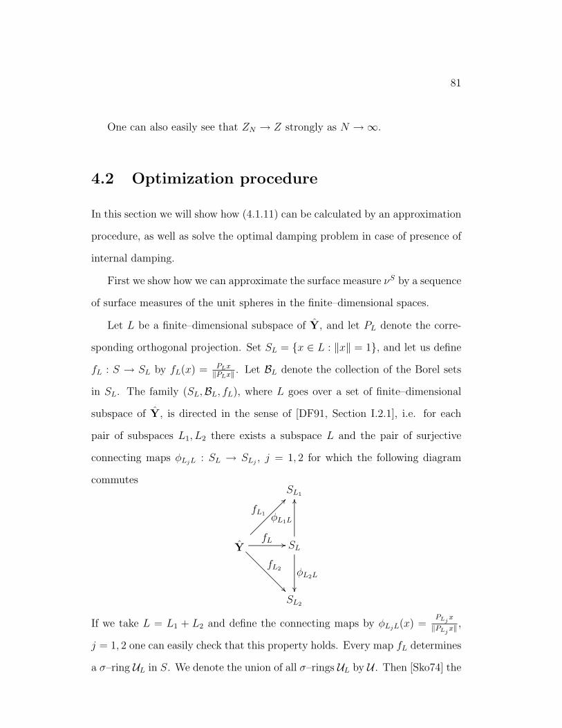
Our next aim is to approximate the operator X. Let YN , Yn ⊂ YN+1
be a chain of finite–dimensional subspaces of Y . Set YN = YN ⊕ YN , which
we treat as a subspace of Y. Let PN be the orthogonal projector from Y to
85
YN . The space YN is equipped with the norm induced from Y. Consider the
sequence of operators AN defined in YN . Assume that AN satisfy the following
assumptions:
(1) there exists λ ∈ ρ(A) ∩n ρ(AN) such that the resolvents converge
(λ− AN)−1PNx → (λ− A)−1x, for all x ∈ Y, (4.2.3)
(2) there exist numbers M ≥ 1 and ω < 0 such that
‖etAN‖ ≤ Meωt for t ≥ 0 and all n ∈ N (4.2.4)
Remark 4.2.1. Generally, we can use any discretization method for the semi-
groups for which some Kato–Trotter–type theorem exists, and (4.2.4) is satisfied
for some ω < 0. In article [GKP01] is given a survey of these methods. Also a
method from [LZ94] can be used. An error estimate for Kato–Trotter theorem
is given in [IK98].
Under these assumptions, one can easily see that the assumptions of Theorem
2.5 from [IM98] are satisfied, which implies that the Lyapunov equation
A∗NX + XAN = −I (4.2.5)
is solvable for all N ∈ N and for the solutions XN we have
XNPNx → Xx for all x ∈ Y.
From the uniform boundedness principle follows supN ‖XN‖ < ∞, hence the
functions ϕN(x) = (XNPNx, x) are bounded and continuous, so they are ν–
measurable functions in Y and ϕN(x) → (Xx, x) holds.
86
This also implies that the functions ϕN(x) = (XN PN x, x) are ν–measurable
and that ϕN(x) → (Xx, x) holds, where XN , PN and x are the corresponding
operators and elements in Y .
We assume that we chose YN in such a way that A′′N = 0, i.e. such that the
”imaginary part” of the operator AN in the sense of the construction given on
the page 77 is zero, so that the operator AN has the following matrix represen-
tation in YN :
AN =
[AN 0
0 AN
]. (4.2.6)
Then
XN =
[XN 0
0 XN
].
Since
G 7→∫
SYN
(Gx, x)νSYN
(dx)
is a linear functional in the space of symmetric matrices G in YN , there exists
a matrix ZN such that
∫
SYN
(Gx, x)νSYN
(dx) = tr(GZN), for all symmetric matrices G. (4.2.7)
As is shown in the Section 2.1 ZN is a symmetric positive semi–definite ma-
trix. Due to the symmetry of the measure νSYN
we have ZN =[
ZN 00 ZN
], hence
tr(XN ZN) = 2tr(XNZN).
In the next section it will be shown how ZN can be calculated.
Now,
tr(XNZN) =1
2
∫
SYN
(XN x, x)νSYN
(dx) =1
2
∫
S
ϕN(x)νS(dx) → 1
2
∫
S
(Xx, x)νS(dx).
(4.2.8)
87
The results of this section can be summarized as follows. Under the usual
assumptions on convergence of the semigroups, we have proved that, instead of
(4.1.11), we can use the following minimization process:
limN→∞
tr(XNZN) → min, (4.2.9)
where XN is the solution of the approximate Lyapunov equation (4.2.5), and
ZN depends only on YN and KR, and can be explicitly computed.
The formula (4.2.9) clearly gives rise to a numerical procedure for the opti-
mization of the damping.
Let us assume that M is compact, and let KR be given by (4.1.12). Let K
be the corresponding operator on Y . By µK we denote the corresponding (in
the sense of Section 4.1) Gaussian measure on Y. We decompose Y = Y1⊕Y2,
where Y1 = N (K)⊥, Y2 = N (K). Then the following generalization of Theorem
2.2.1 holds.
Theorem 4.2.2. Consider the set of operators C such that there exists δ > 0
such that C ≥ δM , i.e. such that
(Cx, x) ≥ δ(Mx, x), for all x ∈ Y . (4.2.10)
Then the optimal damping operators corresponding to the measure µK (in the
sense of ( 4.1.11)) over this set are those operators which have the following
form:
C0 =
2M1/2|Y1 0
0 C1
with C1 being bounded positive definite operator on Y2.
Physical interpretation of the condition (4.2.10) is that the system possesses
internal damping.
88
Proof. First observe that (4.2.10) implies that the corresponding operator A(C)
is uniformly exponentially stable.
Let us denote by µSK the corresponding surface measure. Let us denote by
X(C0) the corresponding solution of the Lyapunov equation (4.1.2). Note that∫S
(X(C0)u, u)µSK(du) does not depend on the choice of C1. Let us assume that
there exists an operator C satisfying the assumption given above, and such that
∫
S
(X(C)u, u)µSK(du) <
∫
S
(X(C0)u, u)µSK(du).
Set YN = spane1, . . . , eN, where ei are normalized eigenvectors of M . We
define YN = YN ⊕ YN ⊂ Y. Let us denote by PN and PN the orthogonal
projectors onto YN and YN , respectively. Set AN = PNA. Then we have
AN := AN(C) =
0 ΩN
−ΩN −ΩNCNΩN
,
where ΩN = M−1/2|YNand CN = PNC.
First we show that the operators AN are stable. Let us assume that AN is
not stable, for some N ∈ N. Then from Proposition 2.1.1 follows that there
exists x ∈ YN such that ΩNx = ωx, for some ω ∈ R, and ΩNCNΩNx = 0. This
implies PNCx = 0, and from 0 = (PNCx, x) = (Cx, PNx) = (Cx, x) we obtain
Cx = 0. Since ω ∈ σ(M), this is in contradiction with Theorem 3.3.9.
One can easily prove
(λ− AN)−1PNx → (λ− A)−1x, for all x ∈ Y, Reλ ≥ 0. (4.2.11)
The relation (4.2.11) implies (4.2.3). Theorem 2.1 from [LZ94] implies that
89
(4.2.4) holds if and only if the following three conditions hold:
supN∈N
Reλ : λ ∈ σ(AN) < 0, (4.2.12)
supReλ≥0,N∈N
‖(λ− AN)−1‖ < ∞, (4.2.13)
there exists Ψ > 0 such that
‖etAN‖ ≤ Ψ, for all t > 0, N ∈ N. (4.2.14)
The relation (4.2.14) is obviously satisfied, since etAN are contractions, and
relation (4.2.13) follows from (4.2.11) and the principle of uniform boundedness.
Assume now that (4.2.12) is not satisfied. Then there exists xN ∈ YN , ‖xN‖ =
1, and λN = αN + iβN , αN < 0, βN ≥ 0 such that
ANxN = λNxN (4.2.15)
and αN → 0.
Let xN = ( uNvN ), uN , vN ∈ YN . Then (4.2.15) can be written as
ΩNvN = λNuN , (4.2.16)
ΩNuN + ΩNCNΩNvN + λNvN = 0. (4.2.17)
The relations (4.2.16) and (4.2.17) imply
λ2NΩ−2
N uN + λNCNuN + uN = 0. (4.2.18)
From (4.2.18) we obtain
αN = −(CNuN , uN)
2‖Ω−1N uN‖2
=(CuN , uN)
2(MuN , uN)→ 0, (4.2.19)
which is in contradiction with (4.2.10).
90
Hence for the subspace sequence YN and approximation operators AN , N ∈N, the formula (4.2.8) holds, which implies that for N large enough there exists
a subspace YN such that the corresponding projections AN(C), AN(C0) and ZN
satisfy
tr(XN(C)ZN) < tr(XN(C0)ZN).
But this is in contradiction with Theorem 2.2.1, since PNC0 ∈ Cmin, Cmin being
the set on which the global minimum is attained.
4.3 Calculation of the matrix ZN
Let us fix some Yn a n–dimensional subspace of Y . Set N = 2n. By YN
we denote the corresponding N–dimensional real subspace of Y constructed
analogously as the space YR in Section 4.1. Let νYNand νS
YNbe Gaussian
measures in YN and SYN, respectively, their construction given in the previous
section. Let KN denote the corresponding covariance operator for the measure
νYN. We decompose YN into YN = Y1
N ⊕Y2N , where Y2
N is the null–space of
the operator KN , and Y1N is the orthogonal complement of Y2
N . Then νYN=
νY1N× νY2
N, where νY1
Nis Gaussian measure with zero mean and covariance
operator PY1NKNPY1
N, PY1
Nbeing the orthogonal projector in Y1
N , and νY2N
is
Dirac measure in Y2N concentrated at zero.
Let us fix a basis in YN such that KN has a matrix representation of the
form
KN =
[K1
N 0
0 0
],
K1N ∈ R2t×2t being positive definite. Then it easily follows that ZN has the
91
matrix representation
ZN =
[Z1
N 0
0 0
].
Therefore, our aim is to compute the matrix Z1N , where Z1
N is such that (4.2.7)
holds for the measure νY1N
in Y1N .
The following formula obviously holds
∫
SY1
N
dνSY1
N=
d
dr
∣∣∣∣∣r=1
∫
x∗x≤r2
νY1N(dx)
. (4.3.1)
The density function of νY1N
with respect to the Lebesgue measure is
p(x) =1
(2π)t√
det K1N
e−1/2x∗K1N−1
x,
hence
∫
x∗x≤r2
νY1N(dx) =
1
(2π)t√
det K1N
∫
x∗x≤r2
e−1/2x∗K1N−1
xdx. (4.3.2)
Let K1N = LL∗ be Cholesky factorization of K1
N , and let L∗L = U∗ΛU be spec-
tral decomposition of L∗L, where Λ = diag(µ1, . . . , µ2t). Note that µ1, . . . , µ2t
are eigenvalues of K1N . By the use of the substitution x = LU∗y, from (4.3.2)
we obtain
∫
x∗x≤r2
νY1N(dx) =
1
(2π)t
∫
y∗Λy≤r2
e−1/2y∗ydy = Pr2t∑
j=1
µjX2j ≤ r2, (4.3.3)
where Xi ∼ N(0, 1) are random vectors with Gaussian distribution N(0, 1)
and Pr denotes the probability function. From the probability theory (see, for
example [Fel66, pp. 48]), follows
Pr2t∑
j=1
µjX2j ≤ r2 = Pr
2t∑j=1
µjχj(1) ≤ r2 = Prm∑
j=1
λjχj(kj) ≤ r2, (4.3.4)
92
where χ(k) denotes the chi–squared distribution with k degrees of freedom, and
λ1, . . . , λm are mutually different eigenvalues of K1N , with their multiplicities (as
eigenvalues) kj. For our construction it is essential to note that kj are always
even.
Let us denote by f and ϕ the probability density function and the charac-
teristic function of∑m
j=1 λjχj(kj), respectively. Then [Fel66, Chapter 15.]
Prm∑
j=1
λjχj(kj) ≤ r2 =
r2∫
0
f(x)dx, (4.3.5)
hence (4.3.1), (4.3.3), (4.3.4) and (4.3.5) imply
∫
SY1
N
dνSY1
N= 2f(1). (4.3.6)
From [Fel66, Chapter 15.] also follows
ϕ(t) =m∏
j=1
ϕχj(kj)(λjt) =m∏
j=1
(1− 2itλj)−kj/2.
Set gj =kj
2. We want to expand ϕ(t) in partial fractions, i.e. to obtain
m∏j=1
(1− 2itλj)−gj =
m∑j=1
gj∑s=1
αjs(1− 2itλj)−s. (4.3.7)
To calculate the coefficients αjs we proceed as follows. Fix j ∈ 1, . . . , m. We
can rewrite (4.3.7) as
(1− 2itλi)−gi
∏
j 6=i
(1− 2itλj)−gj =
gi∑j=1
αis(1− 2itλi)gi +
∑
j 6=i
gj∑w=1
αjw(1− 2itλj)−w.
Multiplying the previous relation by (1 − 2itλi)gi , and by substitution y =
1− 2itλi we get
∏
j 6=i
(λi − λj
λi
+ yλj
λi
)−gj
=
gi∑s=1
αisygi−s + ygi
∑
j 6=i
gj∑w=1
αjw
(λi − λj
λi
+ yλj
λi
)−w
.
(4.3.8)
93
When we take y = 0 in (4.3.8), we obtain
αigi=
∏
j 6=i
(λi − λj
λi
)−gj
,
and when we differentiate both sides of (4.3.8) k times (k = 1, . . . , gi − 1) and
take y = 0, we obtain
αi,gi−k =f
(k)i (0)
k!, where fi(y) =
∏
j 6=i
(λi − λj
λi
+ yλj
λi
)−gj
.
Set
ψi(y) = ln fi(y) = −∑
j 6=i
gj ln
∣∣∣∣λi − λj
λi
+ yλj
λi
∣∣∣∣ .
We calculate the derivatives in zero of the functions ψi and obtain
ψ(k)i (0) = (−1)k(k − 1)!
∑
j 6=i
gj∣∣∣ λi
λj− 1
∣∣∣k
for k ≥ 1.
Now we can calculate the derivatives in zero of the functions fi by use of the
following recursive procedure:
f(1)i (0) = fi(0)ψ
(1)i (0),
f(k+1)i (0) =
k∑
l=0
(k
l
)f
(k−l)i (0)ψ
(l+1)i (0), k = 2, . . . , gi − 1.
After a straightforward calculation we get the following recursive formula for
the coefficients αij, i = 1, . . . , m:
αigi=
∏
j 6=i
(1− λj
λi
)−gj
,
αi,gi−1 = −αigi
∑
j 6=i
gj∣∣∣ λi
λj− 1
∣∣∣, (4.3.9)
αi,gi−k−1 =1
k + 1
k∑
l=0
(−1)l+1αi,gi−k+l
∑
j 6=i
gj∣∣∣ λi
λj− 1
∣∣∣l+1
, k = 1, 2, . . . , gi − 2.
94
Since f(x) = 12π
∞∫−∞
e−itxϕ(t)dt, we have
f(x) =m∑
j=1
gj∑
l=1
αjlfλjχ(2l)(x).
Now the last equation, together with (4.3.6), implies
∫
SYN
dνSYN
= 2m∑
j=1
gj∑
l=1
αjlfλjχ(2l)(1) = 2m∑
j=1
gj∑
l=1
αjl1
λj
fχ(2l)
(1
λj
)
= 2m∑
j=1
gj∑
l=1
αjl1
λlj
1
2l(l − 1)!e− 1
2λj = 2m∑
j=1
e− 1
2λj
gj∑
l=1
αjl1
λlj
1
2l(l − 1)!,
(4.3.10)
since the characteristic function for the chi–squared distribution with k degrees
of freedom is given by
fχ(k)(x) =1
2k/2Γ(k/2)e−
x2 xk/2−1.
Hence we have found a recursive formula for the calculation of the surface
measure of the sphere. It turns out that we can also calculate the entries of the
matrix Z1N by the use of the coefficients αij.
Assume for the moment that the surface measure νSY1
Nis not normalized.
Let X = (Xij) be an arbitrary symmetric matrix in RN . We have
tr(XZ1N) =
∑i,j
Xijtr(Z1NEij) =
∑i,j
Xij
∫
SY1
N
x∗Eijx νSY1
N(dx)
=∑i,j
Xij
∫
SY1
N
xixj νSY1
N(dx),
hence
(Z1N)ij =
∫
SY1
N
xixj νSY1
N(dx), (4.3.11)
95
where Eij denotes the matrix which has all entries zero except for the entry
(i, j) which has value 1. Let K1N−1
= V ΛV ∗ be a spectral decomposition of the
operator K1N−1
, with V orthogonal matrix. By the use of (4.1.10) and by the
substitution x = V y, we obtain∫
SY1
N
xixj νSY1
N(dx) =
1
(2π)t√
det K1N
limε→0
1
2ε
∫
d(x,SY1
N)≤ε
xixje−1/2x∗K1
N−1
xdx
=1
(2π)t√
det K1N
limε→0
1
2ε
∫
d(x,SY1
N)≤ε
(V y)i(V y)je−1/2y∗Λydy.
(4.3.12)
Since (V y)i(V y)j = y∗Eijy, where
Eij = V ∗EijV, (4.3.13)
to compute (Z1N)ij it is enough to calculate
limε→0
1
2ε
∫
d(x,SY1
N)≤ε
yiyje−1/2y∗Λydy. (4.3.14)
From (4.3.2) we obtain
∫
SY1
N
dνSY1
N=
1
(2π)t√
det K1N
∫
SY1
N
e−1/2y∗Λydy. (4.3.15)
By the use of the polar coordinates one can easily check that (4.3.14) equals
∫
SY1
N
yiyje−1/2y∗Λydy.
Note that this integral equals zero in the case i 6= j.
Let ξ : 1, . . . , 2t → 1, . . . , m be the function such that ξ(i) = j implies
µi = λj. Let us fix i ∈ 1, . . . , 2t. Due to the symmetry of the measure νSY1
N,
96
we have ∫
SY1
N
x2i ν
SY1
N(dx) =
∫
SY1
N
x2jν
SY1
N(dx) (4.3.16)
for all j ∈ ξ−1(ξ(i)).
Because of (4.3.15) we can interpret∫
SY1
N
dνSY1
Nas a function in the variables
λ1, . . . , λm, i.e. we denote
F (λ1, . . . , λm) =1
(2π)t√
det K1N
∫
SY1
N
e−1/2Pm
i=1 λiP
j∈ξ−1(ξ(i)) y2j dy.
All partial derivatives of this function exist and
∂
∂λi
F (λ1, . . . , λm) = −1
2
1
(2π)t√
det K1N
∫
SY1
N
∑
j∈ξ−1(ξ(i))
y2j e−1/2y∗Λydy.
The last relation, together with (4.3.16) implies
∫
SY1
N
y2i e−1/2y∗Λydy = −2
(2π)t√
det K1N
kξ(i)
∂
∂λξ(i)
F (λ1, . . . , λm). (4.3.17)
Hence, the relations (4.3.11), (4.3.12), (4.3.15), (4.3.16), and (4.3.17) imply
(Z1N)ij = −2
∑
l
(Eij)ll
kξ(l)
∂
∂λξ(l)
F (λ1, . . . , λm), (4.3.18)
where Eij is given by (4.3.13).
From (4.3.10) follows
F (λ1, . . . , λm) = 2m∑
j=1
e− 1
2λj
gj∑
l=1
αjl1
λlj2
l(l − 1)!,
where αjl is interpreted as a function in variables λ1, . . . , λm. We calculate
∂
∂λi
F (λ1, . . . , λm) = 2m∑
j=1
e− 1
2λj
gj∑
l=1
∂∂λi
αjl
λlj
1
2l(l − 1)!+
1
λ2i
e− 1
2λi
gi∑
l=1
αil
λli
1
2l(l − 1)!−
− 2e− 1
2λi
gi∑
l=1
lαil
λl+1i
1
2l(l − 1)!.
97
Since αjl =f(gj−l)
j (0)
(gj−l)!, we have
∂
∂λi
αjl =1
(gj − l)!
∂
∂ygj−l
∂
∂λi
fj(y, λ1, . . . , λm)
∣∣∣∣y=0
,
where fj is taken as a function in variables y, λ1, . . . , λm. Now
∂
∂λi
fj(y, λ1, . . . , λm) = fj(y, λ1, . . . , λm)∂
∂λi
ln fj(y, λ1, . . . , λm)
= −fj(y, λ1, . . . , λm)∑
l 6=j
gl∂
∂λi
ln
∣∣∣∣λj − λl
λj
+ yλl
λj
∣∣∣∣ .
In the case i 6= j we obtain
∂
∂λi
fj(y, λ1, . . . , λm) = −fj(y, λ1, . . . , λm)gi(y − 1)
λj − λi + yλi
,
and in the case i = j we obtain
∂
∂λi
fi(y, λ1, . . . , λm) = fi(y, λ1, . . . , λm)y − 1
λi
∑
l 6=i
glλl
λi − λl + yλl
.
Let us define functions φji(y) = gi(y−1)λj−λi+yλi
. From the straightforward calculation
we obtain:
φ(k)ji (0) =
(−1)k−1k!giλjλk−1i
(λj − λi)k+1, for k > 0 and φji(0) = − gi
λj − λi
.
Hence in the case i 6= j we have
∂
∂λi
αjl = − 1
(gj − l)!
gj−l∑
k=0
(gj − l
k
)f
(gj−l−k)j (0)φ
(k)ji (0)
= gi
αjl
λj − λi
+ λj
gj−l∑
k=1
(−1)k λk−1i αj,l+k
(λj − λi)k+1
= gi
αjl
λj − λi
+λj
λi(λj − λi)
gj−l∑
k=1
(−1)k
(λi
λj − λi
)k
αj,l+k
.
98
For the case i = j, let us define φi(y) = y−1λi
∑p6=i
gpλp
λi−λp+yλp. Then
φ(k)i (0) = (−1)k−1k!
∑
p 6=i
gpλkp
(λi − λp)k+1, for k > 0 and φi(0) = − 1
λi
∑
p6=i
gpλp
λi − λp
.
Hence
∂
∂λi
αil =1
(gi − l)!
gi−l∑
k=0
(gi − l
k
)f
(gi−l−k)i (0)φ
(k)i (0)
= −αil
λi
∑
p6=i
gpλp
λi − λp
−gi−l∑
k=1
(−1)kαi,l+k
∑
p6=i
gpλkp
(λi − λp)k+1.
After a tedious but straightforward calculation we obtain
∂
∂λi
F (λ1, . . . , λm) =m∑
j=1
gj∑
l=1
βijlαjl, (4.3.19)
where in the case i 6= j we have
βij1 = e− 1
2λjgi
λj(λj − λi), (4.3.20)
and in the case i 6= j, l 6= 1
βijl = 2gie− 1
2λj
λj − λi
(1
2l(l − 1)!
1
λlj
+λj
λi
l−1∑
k=1
(−1)l−k
(λi
λj − λi
)l−k1
λkj
1
2k(k − 1)!
).
(4.3.21)
In the case i = j we have
βii1 =e− 1
2λi
λ2i
(1
2λi
− 1−∑
p6=i
gpλp
λi − λp
), (4.3.22)
and for l 6= 1 we have
βiil = e− 1
2λi1
λl+1i
1
2l(l − 1)!
(1
λi
− 2l − 2∑
p6=i
gpλp
λi − λp
)−
2e− 1
2λi
l−1∑
k=1
1
λki
1
2k(k − 1)!(−1)l−k
∑
p6=i
gpλl−kp
(λi − λp)l−k+1. (4.3.23)
Hence the procedure of the computation of the entries of the matrix Z1N consists
of four steps:
99
(i) compute the coefficients αij using formulae (4.3.9),
(ii) compute the coefficients βijl using (4.3.20), (4.3.21), (4.3.22) and (4.3.23),
(iii) compute ∂∂λi
F (λ1, . . . , λm) using (4.3.19), and
(iv) compute (Z1N)ij using (4.3.18).
This algorithm is numerically unstable in the case in which gi’s are large and
λi is close to λj for some i 6= j. In such cases one can use a Monte Carlo
method of numerical integration to compute the left hand side of (4.3.17). In
our case this method is especially simple and it consists of producing a sequence
of 2t–dimensional random vectors x(i) with normal distribution N(0, Λ) and
calculating∑
i(x(i)j )2/‖x(i)‖2, j = 1, . . . , 2t, where x(i) = (x
(i)1 , . . . , x
(i)2t ).
The serious drawback of Monte Carlo method is its slow convergence which
is of the order O(n−1/2).
There also exist so–called quasi–Monte Carlo methods of integration. They
need significantly less iterations, but the computation of quasi–random vectors
is much more involved.
Note that ZN can be seen as the function of the matrix KN . Also, the
matrices ZN and KN have the same number of zero eigenvalues.
Example 4.3.1. If we take λi = i, i = 1, . . . , 5 and K = diag(λ1, . . . , λ5), then
we obtain Z = diag(0.8105, 0.4258, 0.2887, 0.2183, 0.1756)
Example 4.3.2. Let us take K1 = diag(10, 9, . . . , 2, 1, 1, . . . , 1), where the size
of K is 100. The Monte–Carlo integration with 106 iterations produces Z =
diag(β1, . . . , β100), where β1 = 0.068770, β2 = 0.062182, β3 = 0.055647, β4 =
0.048532, β5 = 0.041262, β6 = 0.034278, β7 = 0.027652, β8 = 0.020550, β9 =
0.013740, β10 = · · · β100 = 0.006900.
100
Example 4.3.3 (Continuation of Example 3.3.2). We will approximate the sys-
tem from Example 3.1.1. The eigenvalues and eigenfunctions of M are cal-
culated in Example 3.3.2. We take N = 50, YN = spanu1, . . . , un, where
ui(x) = sin(n + 12)x are the eigenfunctions of M . We also choose covariance
operator K such that its (infinite–dimensional) matrix in the basis consisting
of the eigenfunctions of M has the form diag(K1, 0, 0, . . .), where K1 is from
Example 4.3.2. It is easy to see that AN(ε) has the form (4.2.6) and is stable.
We calculate
AN(ε) =
0 ΩN
−ΩN −εCN
,
where
ΩN = diag
(1
2, . . . , N +
1
2
)
and
(CN)ij =(−1)i+j
12π(i + 1
2)(j + 1
2).
The matrix AN(ε) is clearly of the form (4.2.6). The function ε 7→ tr(XN(ε)ZN),
where XN(ε) is the solution of the Lyapunov equation
AN(ε)∗X + XAN(ε) = −I,
is plotted on the Figure 4.1.
The optimal damping is attained for ε = 0.38, and for this viscosity we have
tr(XN(ε)ZN) = 1.0275.
If we choose another covariance operator K such that its (infinite–dimensional)
matrix in the basis consisting of the eigenfunctions of M has the form diag(λ1, λ2, . . .),
where λi = λ40+i = 11 − i, i = 1, . . . , 10, λi = 1, 11 ≤ i ≤ 40, and λi = 0,
i > 50, we obtain Figure 4.2.
101
0 0.2 0.4 0.6 0.8 1 1.2 1.4 1.6 1.8 20
2
4
6
8
10
12
14
16
18
20
Figure 4.1: The function ε 7→ tr(XN(ε)ZN)
The optimal damping is attained for ε = 0.53, and for this viscosity we have
tr(XN(ε)ZN) = 1.6618.
4.4 The commutative case
In this section we will treat the case when operators M and C commute. In the
engineering literature this is so–called modal damping case. A very systematic
treatment of the abstract differential equation
y(t) + Ay(t) + By(t) = 0,
in terms of well-posedness of the corresponding Cauchy and boundary value
problem, where A and B are normal commutative operators, is given in [Shk97].
We assume that the operators M and C are such that the corresponding
operator A generates a uniformly exponentially stable semigroup T (t). In this
case the operator X, the solution of the Lyapunov equation (4.1.2) can be
102
0 0.2 0.4 0.6 0.8 1 1.2 1.4 1.6 1.8 20
5
10
15
20
25
30
35
40
45
Figure 4.2: The function ε 7→ tr(XN(ε)ZN)
explicitly calculated. We start with the well-known formula [EN00, Corollary
3.5.15]
T (s)x = limn→∞
1
2πi
ε+in∫
ε−in
eλsR(λ,A)xdλ, x ∈ D(A),
where ε > 0 is arbitrary chosen, n ∈ N and s ≥ 0. Since it is always T (0) = I,
in the sequel we consider only s > 0. Recall that
R(λ,A) =
[1λ(M−1
λ − I) −M−1λ M1/2
M1/2M−1λ −λM1/2M−1
λ M1/2
],
where Mλ = λ2M + λC + I.
Since M and C commute, there exists a bounded selfadjoint operator G
such that the operators M and C are functions of G [AG93, Theorem 76.2],
hence there exists a spectral function E(t) and α, β : R+ → R+ measurable
functions for all Stieltjes measures ([AG93, Section 75] and [KF75, Section
103
36.1]) generated by (E(t)x, x), x ∈ Y , such that
M =
Ξ∫
0
α(t)dE(t), C =
Ξ∫
0
β(t)dE(t),
where Ξ = ‖G‖. Since M and C are bounded, so are also the functions α and β.
We have also α(t) > 0 a.e. It follows that the resolvent R(λ,A) can be written
as
R(λ,A) =
Ξ∫
0
−λα(t)−β(t)λ2α(t)+λβ(t)+1
−√
α(t)
λ2α(t)+λβ(t)+1√α(t)
λ2α(t)+λβ(t)+1−λα(t)
λ2α(t)+λβ(t)+1
dE(t),
hence
T (s) ( xy ) = lim
n→∞1
2πi
ε+in∫
ε−in
eλs
Ξ∫0
−λα(t)−β(t)λ2α(t)+λβ(t)+1
dE(t)x +Ξ∫0
−√
α(t)
λ2α(t)+λβ(t)+1dE(t)y
Ξ∫0
√α(t)
λ2α(t)+λβ(t)+1dE(t)x +
Ξ∫0
−λα(t)λ2α(t)+λβ(t)+1
dE(t)y
dλ.
(4.4.1)
We first treat the case when x, y ∈ R(M1/2).
We want to change the order of integration in (4.4.1) by the use of Fubini
theorem. By the change of variables, we obtain
(T (s) ( x1y1 ) , ( x2
y2 )) = −eεs limn→∞
1
2π
n∫
−n
eiλs
[ Ξ∫
0
p1(λ, t)d(E(t)x1, x2)−
Ξ∫
0
p2(λ, t)d(E(t)y1, x2)+
Ξ∫
0
p2(λ, t)d(E(t)x1, y2)+
Ξ∫
0
p3(λ, t)d (E(t)y1, y2))
]dλ,
where
p1(λ, t) =−(iλ + ε)α(t)− β(t)
(iλ + ε)2α(t) + (iλ + ε)β(t) + 1,
p2(λ, t) =
√α(t)
(iλ + ε)2α(t) + (iλ + ε)β(t) + 1,
p3(λ, t) =−(iλ + ε)α(t)
(iλ + ε)2α(t) + (iλ + ε)β(t) + 1.
104
The integralsn∫
−n
Ξ∫
0
eiλspj(λ, t)d(E(t)x, x)dλ, j = 1, 2, 3, (4.4.2)
can be viewed as a double Lebesgue integrals in R × R+, with the product
measure generated by the standard Lebesgue measure in R and by (real–valued)
Stieltjes measure (E(t)x, x) in R+. Let us now fix n ∈ N. In order to use Fubini
theorem on (4.4.2) we have to prove [KF75, pp. 361,362]:
(i) the functions pj, j = 1, 2, 3 are measurable in the product measure, and
(ii) the integrals
Ξ∫
0
n∫
−n
∣∣eiλspj(λ, t)∣∣ dλ
d(E(t)x, x), j = 1, 2, 3
exist.
To prove (i) it suffices to show that the function g(λ, t) = (iλ + ε)2α(t) + (iλ +
ε)β(t) + 1 is measurable and vanishes only on the set of the measure zero. One
can easily see that the function g does not vanish. Set An = α−1([n, n + 1]),
which is a measurable set in R+. Then R+ = ∪nAn. To prove that g is
measurable, observe that for an arbitrary δ > 0 the following holds
(λ, t) : |g(λ, t)| < δ =⋃n
(An ×
⋃t∈An
λ : |g(λ, t)| < δ)
.
For fixed t ∈ An, one can easily see that λ : |g(λ, t)| < δ is either an empty
set or an open interval or an union of two open intervals, hence always an open
set. It follows that⋃
t∈Anλ : |g(λ, t)| < δ is an open set as a union of open
sets. From this immediately follows that (λ, t) : |g(λ, t)| < δ is measurable
for all δ > 0, hence g is a measurable function.
105
Now we prove (ii). We have
n∫
−n
|pj(λ, t)|dλ =
∫
Υn
|pj(λ, t)|dλ +
∫
Γn
|pj(λ, t)|dλ, (4.4.3)
where Γn is lower semi–circle connecting −n and n, and Υn is the contour
consisting of the segment [−n, n] and the curve Γn. The first integral can be
calculated by the use of residue theorem. The poles of the functions λ 7→ pj(λ, t)
are the zeros of the polynomial g. We calculate the zeros of g. We have
λ1,2 = ±√
4α(t)− β(t)2
2α(t)+ i
2εα(t) + β(t)
2α(t), (4.4.4)
in the case 4α(t) ≥ β(t)2, and
λ1,2 = i2εα(t) + β(t)±
√β(t)2 − 4α(t)
2α(t), (4.4.5)
in the case 4α(t) < β(t)2. Hence the first integral on the right hand side in
(4.4.3) is∫
Υn
|pj(λ, t)|dλ = 0, j = 1, 2, 3. (4.4.6)
To estimate the second integral on the right hand side in (4.4.3) we proceed as
follows.
∫
Γ−n
|pj(λ, t)|dλ = n
2π∫
π
|pj(neiϕ, t)|dϕ ≤ cn2
2π∫
π
dϕ
|g(neiϕ, t)| ,
where c = ε + sup α(t) + sup β(t) + 1, j = 1, 2, 3. We have
g(neiϕ, t) = −n2e2iϕα(t) + ineiϕβ(t) + γ(t) = −n2e2iϕα(t) cos 2ϕ−
− neiϕβ(t) sin ϕ + γ(t) + i(−n2α(t) sin 2ϕ + nβ(t) cos ϕ),
106
where β(t) = 2ε + β(t), γ(t) = ε2α(t) + εβ(t) + 1. Hence
|g(neiϕ, t)|2 =
n4α(t)2+n2β(t)2+γ(t)2−2n3α(t)β(t) sin ϕ−2n2α(t)γ(t) cos 2ϕ−2nβ(t)γ(t) sin ϕ.
Since sin ϕ ≤ 0 for π ≤ ϕ ≤ 2π and β(t) ≥ 0, γ(t) ≥ 1 , we obtain an estimate
|g(neiϕ, t)|2 ≥ n2α(t). (4.4.7)
So, we have obtainedn∫
−n
|pj(λ, t)|dλ ≤ cα(t)−1/2,
where c does not depend on t. Hence the integrals in (ii) exist for all x ∈R(M1/2). We are now in position to use Fubini theorem on (4.4.2), which leads
to
n∫
−n
Ξ∫
0
eiλspj(λ, t)d(E(t)x, x)dλ =
Ξ∫
0
n∫
−n
eiλspj(λ, t)dλ
d(E(t)x, x).
Set f jn(t) =
n∫−n
eiλspj(λ, t)dλ, j = 1, 2, 3. Then
f jn(t) =
∫
Υn
eiλspj(λ, t)dλ +
∫
Γn
eiλspj(λ, t)dλ, (4.4.8)
where Υn and Γn are as in (4.4.3). From (4.4.4) and (4.4.5) we obtain
∫
Υn
eiλspj(λ, t)dλ = 0, j = 1, 2, 3, n ∈ N.
To estimate the second integral in (4.4.8) we use the well–known Jordan lemma
[Gon92, Lemma 9.2] which implies∣∣∣∣∣∣
∫
Γn
eiλspj(λ, t)dλ
∣∣∣∣∣∣≤ c max|pj(λ, t)| : λ ∈ Γn.
107
Now (4.4.7) implies
max|pj(λ, t)| : λ ∈ Γn ≤ (1 + ε)α(t)1/2 +β(t)
α(t)1/2, n ∈ N,
hence |f jn(t)| ≤ f(t), where
f(t) = (1 + ε)α(t)1/2 +β(t)
α(t)1/2.
Since f is integrable for all Stieltjes measures generated by x ∈ R(M1/2), we
can use Lebesgue dominate convergence theorem to obtain
limn→∞
Ξ∫
0
n∫
−n
eiλspj(λ, t)dλ
d(E(t)x, x) =
Ξ∫
0
∞∫
−∞
eiλspj(λ, t)dλ
d(E(t)x, x),
for all x ∈ R(M1/2), in the sense of the principal value integral.
Since (E(t)x, y) can be expressed by the polarization formula
(E(t)x, y) =1
4(E(t)(x+y, x+y)− (E(t)(x−y), x−y)+ i(E(t)(x+ iy), x+ iy)
− i(E(t)(x− iy), x− iy)),
we obtain
(T (s) ( x1y1 ) , ( x2
y2 )) = −eεs 1
2π
[ Ξ∫
0
∞∫
−∞
eiλsp1(λ, t)dλ
d(E(t)x1, x2)−
Ξ∫
0
∞∫
−∞
eiλsp2(λ, t)dλ
d(E(t)y1, x2) +
Ξ∫
0
∞∫
−∞
eiλsp2(λ, t)dλ
d(E(t)x1, y2)+
Ξ∫
0
∞∫
−∞
eiλsp3(λ, t)dλ
d (E(t)y1, y2))
],
for all x1, y1, x2, y2 ∈ R(M1/2).
108
Hence we can write
T (s) ( xy ) = − 1
2πeεs
Ξ∫0
∞∫−∞
eiλsp1(λ, t)dλdE(t)x−Ξ∫0
∞∫−∞
eiλsp2(λ, t)dλdE(t)y
Ξ∫0
∞∫−∞
eiλsp2(λ, t)dλdE(t)x +Ξ∫0
∞∫−∞
eiλsp3(λ, t)dλdE(t)y
(4.4.9)
in the sense of Pettis integral (for the definition and the basic properties see,
for example, [HP57, Chapter 3]). Moreover, the formula (4.4.9) holds for all
x, y ∈ Y , which easily follows from the fact that T (s) is a bounded operator.
Our next aim is to compute the integrals∞∫−∞
eiλspj(λ, t)dλ, j = 1, 2, 3 and
hence to obtain an integral representation of T (s) in terms of the spectral func-
tion E(t). Since pj(·, t) are rational functions such that the degree of the de-
nominator is greater of the degree of the nominator, the standard result from
the calculus (see, for example [Gon92]) implies that
∞∫
−∞
eiλspj(λ, t)dλ = 2πi
∑
λ∈S+
Res(eis·pj(·, t); λ) +1
2
∑
λ∈S0
Res(eis·pj(·, t); λ)
,
where S+ is the set of all poles of the function eis·pj(·, t) in the upper half
plane, and S0 is the set of all real poles of the function eis·pj(·, t). The poles
of the functions eis·pj(·, t) are exactly the zeros of the function g(·, t) which are
calculated in (4.4.4) and (4.4.5).
From the straightforward calculation we obtain:
109
(i) in the case 4α(t) > β(t)2
∞∫
−∞
eiλsp1(λ, t)dλ =− 2πe−sεe−sβ(t)2α(t)
(cos(%(t)s) +
β(t)√4α(t)− β(t)2
sin(%(t)s)
),
∞∫
−∞
eiλsp2(λ, t)dλ =4πe−sεe−sβ(t)2α(t)
√α(t)√
4α(t)− β(t)2sin(%(t)s),
∞∫
−∞
eiλsp3(λ, t)dλ =− 2πe−sεe−sβ(t)2α(t)
(cos(%(t)s)− β(t)√
4α(t)− β(t)2sin(%(t)s)
),
where %(t) =
√4α(t)−β(t)2
2α(t),
(ii) in the case 4α(t) < β(t)2
∞∫
−∞
eiλsp1(λ, t)dλ =− 2πe−sεe−sβ(t)2α(t)
(cosh(%(t)s) +
β(t)√β(t)2 − 4α(t)
sinh(%(t)s)
),
∞∫
−∞
eiλsp2(λ, t)dλ =4πe−sεe−sβ(t)2α(t)
√α(t)√
β(t)2 − 4α(t)sinh(%(t)s),
∞∫
−∞
eiλsp3(λ, t)dλ =− 2πe−sεe−sβ(t)2α(t)
(cosh(%(t)s)− β(t)√
β(t)2 − 4α(t)sinh(%(t)s)
),
where %(t) =
√β(t)2−4α(t)
2α(t),
(iii) and in the (limit) case 4α(t) = β(t)2
∞∫
−∞
eiλsp1(λ, t)dλ =− 2πe−sεe−sβ(t)2α(t)
(1 + s
β(t)
2α(t)
),
∞∫
−∞
eiλsp2(λ, t)dλ =2πe−sεe−sβ(t)2α(t) sα(t)−1/2,
∞∫
−∞
eiλsp3(λ, t)dλ =− 2πe−sεe−sβ(t)2α(t)
(1− s
β(t)
2α(t)
).
110
Let us define functions
sin(t, s) =
sin(%(t)s)√4α(t)−β(t)2
, %(t) ∈ R \ 0,s
2α(t), %(t) = 0,
sinh(e%(t)s)√β(t)2−4α(t)
, %(t) ∈ R \ 0,
and
cos(t, s) =
cos(%(t)s), %(t) ∈ R,
cosh(%(t)s), %(t) ∈ R,.
Then we can write
∞∫
−∞
eiλsp1(λ, t)dλ =− 2πe−sεe−sβ(t)2α(t)
(cos(t, s) + β(t)sin(t, s)
),
∞∫
−∞
eiλsp2(λ, t)dλ =4πe−sεe−sβ(t)2α(t)
√α(t) sin(t, s),
∞∫
−∞
eiλsp3(λ, t)dλ =− 2πe−sεe−sβ(t)2α(t)
(cos(t, s)− β(t)sin(t, s)
),
in all three cases.
Hence we have obtained
T (s) =
Ξ∫
0
e−sβ(t)2α(t)
[cos(t, s) + β(t)sin(t, s) 2
√α(t) sin(t, s)
−2√
α(t) sin(t, s) cos(t, s)− β(t)sin(t, s)
]dE(t).
Now we are in position to use the formula (4.1.3) in order to calculate the
operator X. Set
q1(t, s) = e−sβ(t)2α(t)
(cos(t, s) + β(t)sin(t, s)
),
q2(t, s) = 2e−sβ(t)2α(t)
√α(t) sin(t, s),
q3(t, s) = e−sβ(t)2α(t)
(cos(t, s)− β(t)sin(t, s)
).
111
Then
(X ( x1y1 ) , ( x2
y2 )) =
∞∫
0
( Ξ∫
0
(q1(t, s)2 + q2(t, s)
2)d(E(t)x1, x2)+
+
Ξ∫
0
(q1(t, s)− q3(t, s))q2(t, s)d(E(t)x1, y2)
+
Ξ∫
0
(q1(t, s)− q3(t, s))q2(t, s)d(E(t)y1, x2)+
+
Ξ∫
0
(q3(t, s)2 + q2(t, s)
2)d(E(t)y1, y2)
)ds. (4.4.10)
As before, we would like to change the order of integration in the previous
formula. To do that, it is sufficient to prove that conditions (i) and (ii) from
page 104 are satisfied. The condition (i) is obviously satisfied.
Note that (q1(t, s) − q3(t, s))q2(t, s) ≥ 0 for all t, s > 0, hence all functions
in (4.4.10) are positive. By the use of the standard integration formulae one
obtains
∞∫
0
(q1(t, s)2 + q2(t, s)
2)ds =1
2β(t) +
α(t)
β(t),
∞∫
0
(q1(t, s)− q3(t, s))q2(t, s)ds =1
2
√α(t),
∞∫
0
(q3(t, s)2 + q2(t, s)
2ds =α(t)
β(t).
Hence to be able to change the order of integration we must assume that β(t)−1
is integrable, which implies that the operator C is boundedly invertible. This
implies that a modally damped system decays exponentially if and only if C is
112
boundedly invertible. Therefore, we make this assumption. Then we can write
X =
Ξ∫
0
12β(t) + α(t)
β(t)12
√α(t)
12
√α(t) α(t)
β(t)
dE(t).
Note that this formula is a direct generalization of the formula in the matrix
case given in [Cox98b] (see also [Cox98a], [VBD01]).
Now take any Gaussian measure in Y (in the sense of Section 4.1). Then the
optimal energy decay on the set of boundedly invertible damping operators C
which commute with M is attained for the operator Copt which has a spectral
function βopt such that 12β(t) + 2α(t)
β(t)→ min for all t > 0. One can easily see
that βopt(t) = 2√
α(t), i.e.
Copt = 2M1/2. (4.4.11)
Note that in the finite–dimensional case (4.4.11) reads Copt = 2Ω in the notation
of Chapter 2, where we had shown that in Copt = 2Ω a function C 7→ tr(X(C)Z)
attains its global minimum.
Example 4.4.1. We consider Euler–Bernoulli beam in the presence of viscous
damping term α ∂3
∂x2∂t:
∂2u
∂t2(x, t)− α
∂3u
∂x2∂t(x, t) +
∂4u
∂t4(x, t) = 0, 0 < x < 1, t > 0,
u(0, t) =∂u
∂x(0, t) = u(1, t) =
∂u
∂x(1, t) = 0,
u(x, 0) = u0(x),∂u
∂tu(x, 0) = u1(x),
where α > 0. Multiplying the above differential equation by the smooth test
function v such that v(0) = v(1) = v′(0) = v′(1) = 0, and by partial integration
we obtain
1∫
0
∂2u
∂t2(x, t)v(x)dx−
l∫
0
∂2u
∂x∂t(x, t)v′(x)dx +
l∫
0
∂2u
∂x2(x, t)v′′(x)dx = 0.
113
Hence, the system given above can be written as
µ(u, v) + γ(u, v) + κ(u, v) = 0, for all v ∈ Y ,
where
µ(u, v) =
l∫
0
u(x)v(x)dx,
γ(u, v) = α
1∫
0
u′(x)v′(x)dx,
κ(u, v) =
1∫
0
u′′(x)v′′(x)dx,
and
Y = H20([0, 1]) = u ∈ L2([0, l]) : u′, u′′ ∈ L2([0, l]), u(0) = u′(0) = u(1) = u′(1) = 0.
One can easily see that µ and γ are dominated by κ and that κ > 0, hence we
are in position to use results from Chapter 3. It is clear that M is compact.
The eigenvalues λn of M are the solutions of the equation
cosh λ cos λ = 1,
and the corresponding eigenvectors are
un(x) = cos λnx− cos λnx− βn(sinh λnx− sin λnx),
where
βn =cosh λn − cos λn
sinh λn − sin λn
.
One can check that
infγ(un, un)
λnκ(un, un)> 0,
114
hence, in the light of Remark 3.3.8, the energy of the system has uniform ex-
ponential decay. Since C = αM1/2, the results of this section imply that the
optimal damping is obtained for α = 2.
4.5 Cutting–off in the frequency domain
When we minimize the average total energy, we take into account physical
properties of damping by choosing appropriate Gaussian measure. If we choose
to minimize the maximal total energy, the natural choice is to substitute the
identity operator on the right hand side of the Lyapunov equation (4.1.2) with
some other positive semi–definite operator Q, i.e. instead of X given by (4.1.2)
we can take X which is the solution of the Lyapunov equation
A∗X + XA = −Q, (4.5.1)
where Q is chosen in such a way to take into account the physical properties of
the system. Also, in the case when we minimize the average total energy, we
can instead of (4.1.2) use (4.5.1).
In this section we will give one possible construction of Q in such a way that
it corresponds to smoothing or cutting off in the frequency domain.
We start with the following result which has its own interest. This is a
generalization of the well–known ”frequency domain formula” (2.1.11) to the
infinite–dimensional case.
Proposition 4.5.1. Let A be a generator of an uniformly exponentially stable
semigroup. Then the solution X of the Lyapunov equation ( 4.1.2) satisfies
Xy =1
2π
∞∫
−∞
R(iη, A)∗R(iη, A)ydη, y ∈ D(A), (4.5.2)
115
where the Lebesgue integral above converges strongly in the sense of the principal
value, i.e.
Xy =1
2πlim
Ξ→∞
Ξ∫
−Ξ
R(iη, A)∗R(iη, A)ydη.
Remark 4.5.1. The term ”frequency domain” is used since (4.5.2) could be
understood as integration over amplitudes f of the steady–state solution
xeiwt, x = (iw − A)−1f,
which are the answer to the harmonic load feiwt. The formula (4.1.3) is some-
times refereed as a ”time domain formula”.
Moreover, one can see that the maximal dissipative operator A generates an
uniformly exponentially stable semigroup if and only if the integral on the right
hand side in (4.5.2) converges for all y ∈ D(A).
Proof of Proposition 4.5.1. We start with the Lyapunov equation (4.1.2). We
have
−A∗Xx− iηXx + iηXx−XAx = x, for all x ∈ D(A).
Let us multiply this equation by R(iη, A)∗ on the left and set y = (iη − A)x.
We obtain
XR(iη, A)y + R(iη, A)∗Xy = R(iη, A)∗R(iη, A)y, for all y ∈ Y . (4.5.3)
We have ∞∫
−∞
R(iη, A)xdη = πx, for all x ∈ D(A),
in the sense of the principal value. From the previous relation, (4.5.3) and the
fact that X is bounded, (4.5.2) follows.
116
Now we modify (4.5.2) by putting into the integral in (4.5.2) a smoothing
function g with the following properties:
(i) it is meromorphic in the neighborhood of C− = z ∈ C : Imz ≤ 0 , and
has there finitely many poles,
(ii) it does not have poles in R and g(z) ≥ 0 for all z ∈ R, and
(iii) g|R ∈ L1(R) and zg(z) → 0 as R →∞ for z = Reiϕ, Imz ≤ 0, uniformly
in ϕ.
We start with the relation (4.5.3) which we multiply by 12π
g(η), and we integrate
this relation from −∞ to ∞. We obtain
X1
2π
∞∫
−∞
g(η)R(iη, A)xdη +1
2π
∞∫
−∞
g(η)R(iη, A)∗xdη X =
1
2π
∞∫
−∞
R(iη, A)∗g(η)R(iη, A)xdη.
Since sup‖R(λ,A)‖ : λ ∈ iR < ∞ and g|R ∈ L1(R), the previous formula is
correct. Set
Xg =1
2π
∞∫
−∞
R(iη, A)∗g(η)R(iη, A)dη, (4.5.4)
g(A) =1
2π
∞∫
−∞
g(η)R(iη, A)dη. (4.5.5)
The operator Xg can be seen as a total energy operator smoothed by the function
g. Obviously, one has
Xg = Xg(A) + g(A)∗X.
117
But operator Xg can also be obtained as a solution of a Lyapunov equation.
Indeed, from (4.1.3) follows
A∗Xg + XgA = −(g(A) + g(A)∗). (4.5.6)
This equation has an unique bounded solution since g(A) is a bounded operator.
Since g(A) + g(A)∗ is a selfadjoint operator, so it is Xg. To give any practical
meaning to the formula (4.5.6), the right hand side in (4.5.6) has to be explicitly
solved. Thanks to the property (iii) of the function g, this can be done.
We haven∫
−n
g(η)R(iη, A)dη =
∫
Υn
g(η)R(iη, A)dη +
∫
Γn
g(η)R(iη, A)dη,
where Γn is lower semi–circle connecting −n and n, and Υn is the contour
consisting of the segment [−n, n] and the curve Γn. The first integral on the
right hand side can be calculated by the use of residue theorem.
Let g have poles in points z1, . . . , zk ∈ C− with multiplicities n1, . . . , nk.
Then we can develop function g in the neighborhood of zi, i ∈ 1, . . . , k into
Laurent series
g(η) = βi,−ni(η − zi)
−ni + · · · βi,−1(η − zi)−1 + βi,0 + βi,1(η − zi) + · · ·
On the other hand, we have
R(iη, A) =∞∑
j=0
(−i)j(η − zi)jR(izi, A)j+1,
for all |η − zi| ≤ ‖R(izi, A)‖−1. Hence the coefficient of the term (η − zi)−1 in
the development of the function g(η)R(iη, A) in the neighborhood of zi is given
byni∑
j=1
(−i)j−1βi,−jR(izi, A)j.
118
Hence for n big enough, we have∫
Υn
g(η)R(iη, A)dη = 2πi
k∑i=1
ni∑j=1
(−i)j−1βi,−jR(izi, A)j.
From the Jordan lemma [Gon92, Lemma 9.3] and property (iii) of the function
g it follows
limn→∞
∫
Γn
g(η)R(iη, A)dη = 0,
hence we have obtained
g(A) = 2πi
k∑i=1
ni∑j=1
(−1)j−1βi,−jR(izi, A)j. (4.5.7)
From (4.5.7) it readily follows that g(A) is a rational function of the operator
A. Note also that Xg is always positive definite.
Example 4.5.1. Let g1(η) = 11+0.01η2 . The graph of this function is given in
Figure 4.3. Then g1(A) = 10πR(10, A).
−25 −20 −15 −10 −5 0 5 10 15 20 250.1
0.2
0.3
0.4
0.5
0.6
0.7
0.8
0.9
1
Figure 4.3: The graph of the function g1
We apply weight function g1 in the calculation of the optimal damping from
Example 4.3.3. The function ε 7→ Xg1(ε) is given on the Figure 4.4. Here the
optimal viscosity is ε = 0.3.
119
0 0.2 0.4 0.6 0.8 1 1.2 1.4 1.6 1.8 20
0.05
0.1
0.15
0.2
0.25
0.3
0.35
0.4
0.45
0.5
Figure 4.4: The function ε 7→ Xg1(ε)
Example 4.5.2. Let g2(η) = 0.1η2
(η2+4)(η2+9). The graph of this function is given in
Figure 4.5. Then g2(A) = π45
R(2, A) + 3π40
R(3, A).
We apply weight function g2 in the calculation of the optimal damping from
Example 4.3.3. The function ε 7→ Xg2(ε) is given on the Figure 4.6. Here the
optimal viscosity is ε = 0.31.
120
−25 −20 −15 −10 −5 0 5 10 15 20 250
0.5
1
1.5
2
2.5
3
3.5
4x 10
−3
Figure 4.5: The graph of the function g2
0 0.1 0.2 0.3 0.4 0.5 0.6 0.7 0.80.15
0.2
0.25
0.3
0.35
0.4
0.45
0.5
Figure 4.6: The function ε 7→ Xg2(ε)
Chapter 5
Applications
In this chapter we show how the theory developed in Chapters 3 and 4 can be
applied to the various kinds of damping problems. The applications are grouped
into those which are described by the one–dimensional models, and those which
are described by the multidimensional problems.
In the case of the one–dimensional models, a more complete analysis of the
problems can be given.
In the case of the multidimensional models, the analysis heavily depends on
the geometry of the problems, and we only give more abstract results on how
these problems fit into our theory.
5.1 General remarks
An application of our theory to concrete problems described by the partial
differential equation consists of the following steps.
1. Multiplying by the test function, integrate and then use the boundary con-
ditions to obtain a sesquilinear form representation of the original system of
differential equations, i.e. calculate µ, γ and κ.
121
122
2. Check that κ > 0 (the condition κ(x, x) > 0 can sometimes be bypassed by
taking the orthogonal complement of N (κ), as is done in Section 5.3.2). Show
that quadratic forms µ, γ and κ do generate bounded operators M and C in
some Hilbert space Y . To do this it is enough to check that κ dominates µ and γ,
i.e. that there exists ∆ > 0 such that µ(u, u) ≤ ∆κ(u, u) and γ(u, u) ≤ ∆κ(u, u)
for all u ∈ Y \0. To obtain these inequalities, it usually suffices to apply some
Poincare–type inequality. A brief survey of these inequalities in the connection
with the vibrational systems can be found in [CZ93a].
3. Find necessary (and sufficient, if possible) conditions under which the cor-
responding operator A generates an uniformly exponentially stable semigroup.
If one uses Theorem 3.3.9 one can find the spectrum and the eigenfunctions
of M by solving the system of (partial) differential equations obtained in the
following way:
from the original system of differential equations throw the damping terms
out, and if there are damping terms in the boundary conditions, replace these
boundary conditions with ones for the free end.
In the light of Remark 3.3.8, one can substitute the term ‖Cφn‖ by γ(φn, φn)
in (3.3.40). Sometimes, although C cannot be explicitly calculated, one can
calculate ‖Cx‖, for specific x.
4. Choose some appropriate trace class operator K in YR (in the sense of
Section 4.1). Choose some appropriate subspace sequence Yn ⊂ Y such that
the corresponding operators An satisfy (4.2.3) and (4.2.3), and such that An is of
the form (4.2.6). Calculate Zn either by Monte–Carlo method or by the formula
given in Section 4.3. By the use of some numerical procedure calculate optimal
damping matrices Cn in Y . This gives us a sequence Cn which approximates
123
an optimal damping operator C in Y (and hence an optimal damping form γ).
When it comes to the numerical procedures for approximating the contin-
uous systems, we propose the spectral methods (for the basic introduction to
these methods, see [Tre00]). Experiments had shown ([DT96], [Tre97]) that the
finite difference and finite element methods frequently behave poorly on prob-
lems for vibrational systems, in contrast with the spectral methods. Only in
the cases of the complex geometry of the problem, the finite element methods
should be used.
5.2 One–dimensional problems
5.2.1 Cable with a tip mass
We consider a vertical cable which is pinched at the upper end and with a tip
mass attached at the lower end, where a control force linear feedback depending
on the velocity is applied.
The dynamics is described by the following system [MRC94] (see also [BX00])
∂2u
∂t2(x, t)− ∂2u
∂x2(x, t) = 0, 0 < x < 1, t > 0,
u(0, t) = 0,
∂u
∂x(1, t) + m
∂2u
∂t2(1, t) + α
∂u
∂t(1, t) = 0,
u(x, 0) = u0(x),∂u
∂tu(x, 0) = u1(x),
where we assume m,α > 0.
Multiplying the above differential equation by the smooth test function v
124
such that v(0) = 0 and by partial integration we obtain
1∫
0
∂2u
∂t2(x, t)v(x)dx + m
∂2u
∂t2(1, t)v(1) + α
∂u
∂t(1, t)v(1) +
1∫
0
∂u
∂x(x, t)v′(x)dx = 0.
Hence, the system given above can be written as
µ(u, v) + γ(u, v) + κ(u, v) = 0, for all v ∈ Y , (5.2.1)
where
µ(u, v) =
1∫
0
u(x)v(x)dx + mu(1)v(1),
γ(u, v) = αu(1)v(1),
κ(u, v) =
1∫
0
u′(x)v′(x)dx,
and
Y = u ∈ L2([0, 1]) : u′ ∈ L2([0, 1]), u(0) = 0.
Now from Examples 3.1.1 and 3.1.2 immediately follows that the forms µ, γ
and κ give rise to the bounded operators M and C given by
(Mu)(x) =
1∫
0
G(x, ξ)u(ξ)dξ + mu(1)x,
(Cu)(x) = αu(1)x,
where
G(x, ξ) =
x, x ≤ ξ,
ξ, x ≥ ξ. (5.2.2)
The operator M is compact and one can calculate its eigenvalues and eigen-
functions. We obtain that the eigenvalues λn are the solutions of the equation
mλ−1/2 tan λ−1/2 = 1, (5.2.3)
125
and the corresponding eigenfunctions are
un(x) = sin λ−1/2n x. (5.2.4)
By a straightforward, but tedious computation we obtain
inf‖Cun‖‖Mun‖ = 0,
hence the energy of the system does not have an uniform exponential decay,
which is a well-known fact [LM88].
5.2.2 Vibrating string with viscous and boundary damp-
ing
We consider the vibrating string with viscous and boundary damping given by:
∂2u
∂t2(x, t) + α
∂u
∂t(x, t)− β
∂3u
∂x2∂t(x, t)− ∂2u
∂x2(x, t) = 0, 0 < x < π, t > 0,
u(0, t) = 0,
∂u
∂x(1, t) + ε
∂u
∂t(1, t) = 0, (5.2.5)
u(x, 0) = u0(x),∂u
∂tu(x, 0) = u1(x),
where we assume α, β, ε ≥ 0.
Multiplying the above differential equation by the smooth test function v
such that v(0) = 0, by partial integration, and by differentiating (5.2.5) we
obtain
π∫
0
∂2u
∂t2(x, t)v(x)dx + α
π∫
0
∂u
∂t(x, t)v(x)dx + β
π∫
0
∂2u
∂x∂t(x, t)v′(x)dx+
π∫
0
∂u
∂x(x, t)v′(x)dx + ε
∂u
∂t(π, t)v(π) + ε
∂2u
∂t2(π, t)v(π) = 0.
126
Hence, the system given above can be written as (5.2.1), where
µ(u, v) =
π∫
0
u(x)v(x)dx + εu(π)v(π),
γ(u, v) = α
π∫
0
u(x)v(x)dx + β
π∫
0
u′(x)v′(x)dx + εu(π)v(π),
κ(u, v) =
π∫
0
u′(x)v′(x)dx,
and
Y = u ∈ L2([0, 1]) : u′ ∈ L2([0, 1]), u(0) = 0.
Now from Examples 3.1.1 and 3.1.2 immediately follows that the forms µ, γ
and κ give rise to the bounded operators M and C given by
(Mu)(x) =
1∫
0
G(x, ξ)u(ξ)dξ + εu(1)x,
(Cu)(x) = α
1∫
0
G(x, ξ)u(ξ)dξ + εu(1)x + βu(x),
where the function G is given by (5.2.2).
If α > 0 or β > 0 then the system obviously has uniform decay of energy.
In the case α = 0, β = 0 and ε > 0 we are in position of Example 3.1.1, hence
we also have an uniform exponential decay of energy.
From the previous subsection we know that the eigenvalues λn of M are
the solutions of the equation (5.2.3) where instead of m stands ε, and the
corresponding eigenfunctions are given by (5.2.4).
Now we will find an approximation of the optimal parameters. We take
ε = 12, and optimize over α and β. We take N = 30, YN = spanu1, . . . , uN,
where ui are the eigenfunctions of M . We also choose covariance operator
127
K such that its (infinite–dimensional) matrix in the basis consisting of the
eigenfunctions of M has the form diag(K1, 0, 0, . . .), where K1 is from Example
4.3.2. It is easy to see that the assumptions from Section 4.2 are satisfied. We
calculate
AN(ε) =
[0 ΩN
−ΩN −CN(α, β)
],
where
ΩN = diag (τ1, . . . , τN) ,
with τ1 < . . . < τN positive solutions of the equation
τ tan τ − 2 = 0,
and
CN(α, β) = αΩ−2N + βI +
1
2(1− α)C0,
where
(C0)ij =sin τiπ sin τjπ
τiτj
√(1
2π + 1
4τisin 2τiπ)(1
2π + 1
4τjsin 2τjπ)
.
The matrix AN(α, β) is clearly of the form (4.2.6). The function (α, β) 7→tr(XN(α, β)ZN), where XN(α, β) is the solution of the Lyapunov equation
AN(α, β)∗X + XAN(α, β) = −I,
is plotted on the Figure 5.1.
The optimal damping is attained for α = 0.5, β = 0.7.
128
00.5
11.5
2
0
0.5
1
1.5
20
0.005
0.01
0.015
0.02
0.025
0.03
0.035
Figure 5.1: The function (α, β) 7→ tr(XN(α, β)ZN)
5.2.3 Clamped Rayleigh beam with viscous damping
We consider a clamped Rayleigh beam in the presence of viscous damping term
2 ∂∂x
(a ∂2u
∂t∂x
). The corresponding system is given by [Rao97] (see also [Rus86])
∂2u
∂t2(x, t)− α2 ∂4u
∂x2∂t2(x, t) +
∂4u
∂t4(x, t)− 2
∂
∂x
(a
∂2u
∂t∂x
)(x, t) = 0, 0 < x < 1, t > 0,
u(0, t) =∂u
∂x(0, t) = u(1, t) =
∂u
∂x(1, t) = 0,
u(x, 0) = u0(x),∂u
∂tu(x, 0) = u1(x),
where α2 > 0 is the coefficient of the moment of inertia, and where potential
a ∈ L∞([0, 1]) is a positive function.
Multiplying the above differential equation by the smooth test function v
129
such that v(0) = v(1) = v′(0) = v′(1) = 0 and by partial integration we obtain
l∫
0
∂2u
∂t2(x, t)v(x)dx + α2
1∫
0
∂3u
∂t2∂x(x, t)v′(x)dx+
1∫
0
∂2u
∂x2(x, t)v′′(x)dx + 2
1∫
0
a(x)∂2u
∂t∂x(x, t)v′(x)dx = 0.
Hence, the system given above can be written as (5.2.1), where
µ(u, v) =
1∫
0
u(x)v(x)dx + α2
1∫
0
u′(x)v′(x)dx,
γ(u, v) = 2
1∫
0
a(x)u′(x)v′(x)dx,
κ(u, v) =
1∫
0
u′′(x)v′′(x)dx,
and
Y = u ∈ L2([0, 1]) : u′, u′′ ∈ L2([0, 1]), u(0) = u′(0) = u(1) = u′(1) = 0.
Then one can easily see that the forms µ and γ are dominated by κ. κ > 0 is
obvious. The operator M is compact [Rao01, Proposition 2.1].
In the case a(x) ≥ δ > 0 the operator C is uniformly positive, and the
system has uniform exponential decay of energy.
The eigenvalues λn of M are the solutions of the equation
cosh p+λ cos p−λ
α2
2√
λsinh p+
λ sin p−λ = 1,
where
p+λ =
√α2 +
√α4 + 4λ
2, p−λ =
√√α4 + 4λ− α2
2.
130
The corresponding eigenfunctions are
un(x) = cosh p+λn
x−cos p−λnx− cosh p+
λn− cos p−λn
sinh p+λn− p+
λn
p−λn
sin p−λn
(sinh p+
λnx− α2
√λn
sin p−λn
).
So, in the general case, the system has uniform exponential decay of energy if
a is such that
inf
1∫0
a(x)u′n(x)2dx
λn
1∫0
u′′n(x)2dx
> 0,
where λn and un are given above.
5.2.4 Euler–Bernoulli beam with boundary damping
We consider a Euler–Bernoulli beam which is pinched at x = 0 and has a
damper and the spring attached at x = 1. The corresponding equations are
∂2u
∂t2(x, t) +
∂2
∂x2
(EI
∂2u
∂x2
)(x, t) = 0, t > 0, x ∈ (0, 1),
u(0, t) =∂u
∂x(0, t) = 0,
∂
∂x
(EI(x)
∂2u
∂x2
)(1, t) = ku(1, t) + c
∂u
∂t(1, t),
∂2u
∂x2(1, t) = 0,
u(x, 0) = u0(x),∂u
∂tu(x, 0) = u1(x),
where c > 0 and k > 0 are damping and spring coefficient, respectively.
Multiplying the above differential equation by the smooth test function v
such that v(0) = v′(0) = 0 and by partial integration we obtain
1∫
0
∂2u
∂t2(x, t)v(x)dx+
1∫
0
EI(x)∂2u
∂x2(x, t)v′′(x)dx+ku(1, t)v(1)+c
∂u
∂t(1, t)v(1) = 0.
131
Hence, the system given above can be written as (5.2.1), where
µ(u, v) =
1∫
0
u(x)v(x)dx,
γ(u, v) = cu(1)v(1),
κ(u, v) =
1∫
0
EI(x)u′′(x)v′′(x)dx + ku(1)v(1),
and
Y = u ∈ L2([0, 1]) : u′, u′′ ∈ L2([0, 1]), u(0) = u′(0) = 0.
We assume EI(x) ≥ δ > 0. Then one can easily see that the forms µ and γ are
dominated by κ. κ > 0 is obvious. Since M is compact, the eigenvalues λn tend
to zero for n →∞. Let us denote the corresponding eigenvalues by un. Then
γ(un, un)
λnκ(un, un)=
cun(1)2
λn
(1∫0
EI(x)u′′n(x)2dx + kun(1)2
) ≥ c
kλn
.
This implies that the system has a uniform exponential decay of energy if c > 0.
5.2.5 Euler–Bernoulli beam with Kelvin–Voigt damping
We assume that the Euler–Bernoulli beam is clamped at x = 0, and free at
x = l. The dynamics of transverse vibration is described by the following
132
system [IN97]:
∂2u
∂t2(x, t) +
∂2
∂x2
(EI
∂2u
∂x2+ DI
∂3u
∂x2∂t
)(x, t) = 0, t > 0, x ∈ (0, l),
u(0, t) =∂u
∂x(0, t) = 0,
EI(x)∂2u
∂x2(x, t) + DI(x)
∂3u
∂x2∂t(x, t)
∣∣∣∣x=l
= 0,
∂
∂x
(EI
∂2u
∂x2+ DI
∂3u
∂x2∂t
)(x, t)
∣∣∣∣x=l
= 0,
u(x, 0) = u0(x),∂u
∂tu(x, 0) = u1(x).
In the above system EI is the stiffness coefficient and DI is the damping coef-
ficient of the beam material.
Multiplying the above differential equation by the smooth test function v
such that v(0) = v′(0) = 0 and by partial integration we obtain
l∫
0
∂2u
∂t2(x, t)v(x)dx+
l∫
0
DI(x)∂3u
∂x2∂t(x, t)v′′(x)dx+
l∫
0
EI(x)∂2u
∂x2(x, t)v′′(x)dx = 0.
Hence, the system given above can be written as (5.2.1), where
µ(u, v) =
l∫
0
u(x)v(x)dx,
γ(u, v) =
l∫
0
DI(x)u′′(x)v′′(x)dx,
κ(u, v) =
l∫
0
EI(x)u′′(x)v′′(x)dx,
and
Y = u ∈ L2([0, l]) : u′, u′′ ∈ L2([0, l]), u(0) = u′(0) = 0.
Let us assume that the stiffness and damping coefficients satisfy
EI(x) ≥ δ > 0 and EI ∈ L∞([0, l]) and DI ∈ L∞([0, l]).
133
Then one can easily see that the forms µ and γ are dominated by κ. κ > 0 is
obvious. Hence we are in position to apply results from the Section 3.3. One
can easily see that
‖Cu‖2 =
l∫
0
DI(x)2
EI(x)|u′′(x)|2dx.
Also, M is obviously a compact operator. Let us denote by λn the eigenvalues
of M . In the general case, the system need not have a uniform exponential
decay of the energy.
In the simplest case EI(x) = 1, the eigenvalues λn are the solutions of the
following equation:
(cosh λl + cos λl)2 = 1 + cosh λl cos λl,
and the eigenfunctions un are given by
un(x) = cosh λnx− cos λnx + βn(sinh λnx− sin λnx),
where
βn =sinh λnl − sin λnl
cosh λnl + cos λnl.
Then a sufficient condition for the uniform exponential decay of the energy is
DI ≥ p > 0, which easily follows from the Remark 3.3.8.
5.3 Multidimensional problems
5.3.1 Higher dimensional hyperbolic systems
The hyperbolic system which has received the most attention from the control-
lability viewpoint is the generalized wave equation
ρ(x)∂2u
∂t2(x, t)−∇(A(x)∇u)(x, t)+q(x)u(x, t) = 0 for x ∈ Ω, t ≥ 0, (5.3.1)
134
where real valued coefficients in (5.3.1) satisfy the following: p, q ∈ L∞(Ω) and
ρ(x) ≥ ρ0 > 0, q(x) ≥ 0 in Ω; A(x) = (aij(x))N1 satisfies uniform elipticity
condition, its entries have Lipschitz continuous second derivatives, and Ω is a
bounded open connected subset in Rn with the Lipschitz boundary ∂Ω.
We divide the boundary ∂Ω in two parts, Γ0 and Γ1, with Γ1 6= ∅, Γ2 6= ∅and Γ0 relatively open in ∂Ω.
We impose the following boundary conditions:
u(x, t) = 0, x ∈ Γ0,
β(x)∂u
∂t(x, t) + A(x)∇u(x, t) · ν(x) = 0, x ∈ Γ1,
where β(x) ≥ β0 > 0 and ν is the unit normal of ∂Ω pointing towards the
exterior of Ω. The problem of decay of the solutions and the problem of finding
the optimal β has caught the attention of many researches (see, for example,
[Rus78], [Lag83], [Tri89]). By the use of partial integration and divergence
theorem, this system can be written in the form (5.2.1) where
µ(u, v) =
∫
Ω
u(x)v(x)dx,
γ(u, v) =
∫
Γ1
β(x)u(x)v(x)dx,
κ(u, v) =
∫
Ω
(∇v(x))∗A(x)∇u(x)dx +
∫
Ω
q(x)u(x)v(x)dx,
and
Y = u ∈ H1(Ω) : u(0) = 0 on Γ0.
It can be shown ([Lag83, Proof of the Theorem 1], [CZ93a, Example 3.5.1]
and [Rus78, pp. 682]) that under above assumptions forms µ and γ are domi-
nated by κ. κ > 0 is obvious. Hence, the results from Chapter 3 are applicable.
135
Even in the simplest case A(x) = 1, ρ(x) = 1 and q(x) = 0, the exact
calculation of the eigenvalues of M is not possible except in the cases when
Ω has particulary simple geometry, but even in this cases the computation is
usually lengthy and tedious (see, for example, [CFNS91, Section 3.] and [CZ93b,
Section 2.6]).
5.3.2 A problem in dissipative acoustics
In this section we are studying linear oscillations of an acoustic (i.e. inviscid,
compressible, barotropic) fluid contained in a rigid cavity, with some or all of
its walls covered by a thin layer of viscoelastic material able to absorb part of
the acoustic energy of the fluid.
In recent years large attention has been paid to this kind of problem, mainly
related to the goal of decreasing the level of noise in aircraft or cars (for exam-
ple, a typical problem in aeronautical engineering is the problem of reducing
the noise produced by propellers inside an aircraft by means of thin layers of
viscoelastic material). A typical acoustic insulating material is glasswool.
We denote by Ω ⊂ Rn, n = 2 or n = 3 the domain occupied by the fluid,
which we suppose polyhedral, with boundary ∂Ω = ΓA ∪ ΓR, ΓA =⋃J
j=1 Γj,
with Γj being all the different faces of Ω covered by the damping material, is
called the ”absorbing boundary”. ΓR is the union of the remaining faces and
we call it the ”rigid boundary”. We assume that ΓA is not empty. The unit
outer normal vector along ∂Ω is denoted by ν. The equations for our problem
136
are [BDRS00]
ρ∂2U
∂t2+∇P = 0 in Ω, (5.3.2)
P = −ρc2divU in Ω, (5.3.3)
P = αU · ν + β∂U
∂t· ν on ΓA, (5.3.4)
U · ν = 0 on ΓR, (5.3.5)
where U is the displacement vector, P is the fluid pressure, ρ the fluid density,
and c the acoustic speed.
The equation (5.3.4) models the effect of viscoelastic material: the fluid
pressure on the boundary is in equilibrium with the response of the absorbing
walls. This response consists of two terms: the first one is proportional to the
normal component of the displacements and acoustics for the elastic behavior
of the material, whereas the second one is proportional to the normal velocity
and models the viscous damping.
The damped vibration modes of the fluid are complex solutions of (5.3.2)–
(5.3.5) of the form U(x, t) = eλtu(x) and P (x, t) = eλtp(x). They can be found
by solving the following quadratic problem:
∫
Ω
ρc2divu divφ+
∫
ΓA
αu·ν φ·ν+λ
∫
ΓA
β u·ν φ·ν+λ2
∫
Ω
ρuφ = 0, for all φ ∈ V ,
(5.3.6)
where
V =φ ∈ H(div, Ω) : φ · ν ∈ L2(∂Ω) and φ · ν = 0 on ΓR
,
endowed with its natural norm
‖φ‖V =(‖φ‖2
div,Ω + ‖φ‖2ΓA
)1/2.
137
Here
H(div, Ω) = φ ∈ L2(Ω) : divφ ∈ L2(Ω)
is a Hilbert space (see, for example [GR86]) with the norm
‖φ‖div,Ω =(‖φ‖2
Ω + ‖div φ‖2Ω
)1/2.
Let us define three (symmetric) sesquilinear forms in V
µ(u,v) =
∫
Ω
ρuv,
γ(u,v) =
∫
ΓA
β u · ν v · ν,
κ(u,v) =
∫
Ω
ρc2divu divv +
∫
ΓA
αu · ν v · ν.
Then (5.3.6) becomes
λ2µ(u,v) + λγ(u,v) + κ(u,v) = 0, for all v ∈ V . (5.3.7)
Obviously, λ = 0 is an eigenvalue, with corresponding eigenspace
K = u ∈ V : div u = 0 on Ω and u · ν = 0 on ∂Ω,
so as the space in which we will operate we take [GR86]
Y := V ª K = u ∈ V : u = ∇ϕ for ϕ ∈ H1(Ω).
From [BDRS00, Lemma 2.2] follows that the quadratic form κ generates a norm
in Y which is equivalent to ‖·‖V . Then clearly the forms µ and γ are dominated
by κ, hence the corresponding operators M and C constructed in Section 3.1
are bounded. Moreover, from [BDRS00, Lemma 3.1] follows that M is compact.
Hence we can apply results from Section 3.3 to this problem. In the special
cases when the geometry of Ω is simple, the eigenvalues and eigenvectors of
138
M can be found by the separation of variables technique (for the case when
n = 2 and Ω is rectangular see [BR99], and for the case when n = 3 and Ω is
rectangular box see [BHNR01]).
But even in these simple cases, the computation of the operator C is heavily
involved, since the operator C cannot be written in a closed form. To gain a
little more insight in the structure of C, observe that βα
is an eigenvalue of C
with the corresponding eigenspace F = u ∈ Y : div u = 0. Also, one can
check that F⊥ = u ∈ Y : u · ν is constant on ΓA, and since Cu depends only
on u · ν in F⊥, C|F⊥ has one–dimensional range.
Appendix A
Semigroup theory
In the appendix we introduce the basic concepts and results of the semigroup
theory which we use in this thesis.
The classic reference on semigroup theory is [HP57]. Standard references
are also [Paz83], [EN00], [Gol85] and [BM79].
Let X be a Hilbert space. The family of bounded linear operators T (t),
t ≥ 0 in X is said to be a semigroup of operators in X if
(i) T (0) = I,
(ii) T (t + s) = T (t)T (s) for all t, s ≥ 0.
The semigroup T (t), t ≥ 0 is said to be strongly continuous if it is continuous
in the strong operator topology. Due to the property (ii) this is equivalent to
(iii) limt0 ‖T (t)x− x‖ = 0 for each x ∈ X .
A strongly continuous semigroup is sometimes called as C0 semigroup1.
The infinitesimal generator of T (t), or briefly the generator, is the linear
1The symbol C0 abbreviates ”Cesaro summable of order 0”.
139
140
operator A with domain D(A) defined by
D(A) = x ∈ X : limt0
1
t(T (t)x− x) exists,
Ax = limt0
1
t(T (t)x− x), x ∈ D(A).
The generator is always a closed and densely defined operator. The generator
uniquely determines the semigroup.
Proposition A.1 ([EN00]). For every strongly continuous semigroup T (t),
there exist constants ω ∈ R and M ≥ 1 such that
‖T (t)‖ ≤ Meωt for all t ≥ 0. (A.1)
The infimum of all exponents ω for which an estimate of the form (A.1)
holds for a given strongly continuous semigroup plays an important role in the
semigroup theory. For a strongly continuous semigroup T (t) generated by A we
call
ω(A) = infω : ∃M ≥ 1 such that ‖T (t)‖ ≤ Meωt for all t ≥ 0
its growth bound (or type).
Moreover, a semigroup is called contractive if ω = 0 and M = 1 is possible,
and uniformly exponentially stable if its growth bound is negative.
Remark A.1. Let A be generator of strongly continuous semigroup T (t). The
number
s(A) = supReλ : λ ∈ σ(A)
is called the spectral bound of the semigroup T (t). In the finite–dimensional
case s(A) = ω(A) holds, but in general we have only s(A) ≤ ω(A).
141
In the sequel we will give characterizations of the generators of contractive
and uniformly exponentially stable semigroups.
Let A be a linear operator with the dense domain. The operator A is called
dissipative operator if Re(Ax, x) ≤ 0 for all x ∈ D(A). A dissipative operator
which extends a dissipative operator A is called a dissipative extension of A.
An operator A is said to be maximal dissipative if its only dissipative extension
is A itself.
Proposition A.2. If A is a dissipative operator and R(A − λ) = X for some
λ, Reλ > 0, then A is maximal dissipative.
Theorem A.3 (Lumer–Phillips). Let A be a linear operator with dense do-
main. Then A generates a contractive semigroup if and only if A is maximal
dissipative.
Theorem A.4 ([EN00], pp. 302). A strongly continuous semigroup T (t) in
a Hilbert space is uniformly exponentially stable if and only if the half plane
λ ∈ C : Reλ > 0 is contained in the resolvent set ρ(A) of the generator A
with the resolvent satisfying
supReλ>0
‖R(λ)‖ < ∞.
From the previous theorem one can obtain
Corollary A.5 ([CHA+87], Theorem 9.6). If T (t) is a strongly continuous
semigroup in a Hilbert space with generator A, then its growth bound is given
by
ω(A) = infβ ∈ R : sups∈R
‖R(β + is)‖ < ∞.
142
The following two results are also needed.
Proposition A.6 ([Gol85]). Let A generate strongly continuous semigroup
T (t). Then T (t) = 0 for all t ≥ t0, where t0 > 0, if and only if σ(A) = ∅ and
there exists a constant M such that
‖R(α + iβ, A)‖ ≤ M max1, e−αt0
for all α + iβ ∈ C.
The following Lemma is a well-known result, but we give the proof because
we were not able to find an appropriate reference.
Lemma A.7. Let T (t) ba a uniformly exponentially stable semigroup with gen-
erator A. Assume that
‖R(iβ)‖ ≤ M, for all β ∈ R,
for some M > 0. Then ω(A) ≤ − 1M
.
Proof. From [Wei76, Satz 5.14] follows λ ∈ ρ(A) if |Reλ| < 1M
and
(λ− A)−1 =∞∑
n=0
(−1)n(Reλ)n(iImλ− A)−n−1, for |Reλ| < 1
M.
Hence
‖(λ− A)−1‖ ≤∞∑
n=0
|Reλ|nMn+1 =M
1− |Reλ|M , for |Reλ| < 1
M.
Now Corollary A.5 implies ω(A) ≤ − 1M
.
Let A be a linear operator, and let u0 ∈ X . Consider the differential equation
given by
u(t) = Au(t) for t ≥ 0,
u(0) = u0.(A.2)
143
A function u : [0,∞) → X is called a classical solution of (A.2) if u is contin-
uously differentiable with respect to X , u(t) ∈ D(A) for all t ≥ 0 and (A.2)
holds.
A continuous function u : [0,∞) → X is called a mild solution of (A.2) ift∫
0
u(s)ds ∈ D(A) for all t ≥ 0 and
u(t) = A
t∫
0
u(s)ds + u0.
The following theorem deals with the question of existence and uniqueness of the
solution of the problem (A.2), called the abstract Cauchy problem associated
to A with the initial value u0.
Theorem A.8 ([EN00], Propositions 6.2 and 6.4). Let A be the generator
of the strongly continuous semigroup T (t). Then, for every u0 ∈ X , the function
u : t 7→ u(t) := T (t)u0 (A.3)
is the unique mild solution of (A.2).
Moreover, for every u0 ∈ D(A), the function (A.3) is the unique classical
solution of (A.2).
Bibliography
[AG93] N. I. Akhiezer and I. M. Glazman, Theory of linear operators in
Hilbert space, Dover Publications Inc., New York, 1993.
[BB80] D. E. Beskos and B. A. Boley, Critical damping in linear discrete
dynamic systems, ASME J. Appl. Mech. 47 (1980), 627–630.
[BDMS98] B. P. Belinskiy, J. P. Dauer, C. Martin, and M. A. Shubov, On
controllability of an elastic string with a viscous damping, Numer.
Funct. Anal. Optim. 19 (1998), no. 3-4, 227–255.
[BDRS00] A. Bermudez, R. G. Duran, R. Rodrıguez, and J. Solomin, Finite
element analysis of a quadratic eigenvalue problem arising in dissi-
pative acoustics, SIAM J. Numer. Anal. 38 (2000), no. 1, 267–291.
[Bes76] D. E. Beskos, The efect of damping on the vibration–stability relation
of linear systems, Mech. Res. Comm. 3 (1976), 373–377.
[BHNR01] Alfredo Bermudez, L. Hervella-Nieto, and Rodolfo Rodrıguez, Fi-
nite element computation of the vibrations of a plate-fluid system
with interface damping, Comput. Methods Appl. Mech. Engrg. 190
(2001), no. 24-25, 3021–3038.
[BM79] Aldo Belleni-Morante, Applied semigroups and evolution equations,
The Clarendon Press Oxford University Press, New York, 1979.
145
146
[BR99] Alfredo Bermudez and Rodolfo Rodrıguez, Modelling and numerical
solution of elastoacoustic vibrations with interface damping, Inter. J.
Numer. Methods Engrg. 46 (1999), no. 10, 1763–1779.
[Bra98] Katrin Brabender, Optimale Dampfung von Linearen
Schwingungssystemen, Ph.D. thesis, Fernuniversitat Hagen,
1998.
[BS72] R. H. Bartels and G. W. Stewart, Solution of the matrix equation
AX + XB = C, Comm. ACM 15 (1972), 820–826.
[BX00] Guo Baozhu and Cheng-Zhong Xu, On the spectrum–determined
growth condition of a vibration cable with a tip mass, IEEE Trans.
Automatic Control 45 (2000), no. 1, 89–93.
[CFNS91] G. Chen, S. A. Fulling, F. J. Narcowich, and S. Sun, Exponential de-
cay of energy of evolution equations with locally distributed damping,
SIAM J. Appl. Math. 51 (1991), no. 1, 266–301.
[CHA+87] Ph. Clement, H. J. A. M. Heijmans, S. Angenent, C. J. van Duijn,
and B. de Pagter, One-parameter semigroups, North-Holland Pub-
lishing Co., Amsterdam, 1987.
[CNRV02] Steven J. Cox, Ivica Nakic, Annette Rittmann, and Kresimir Veselic,
Minimization of energy of a damped system, 2002.
[Cox98a] Steven J. Cox, Designing for optimal energy absorption. II. The
damped wave equation, Control and estimation of distributed param-
eter systems (Vorau, 1996), Birkhauser, Basel, 1998, pp. 103–109.
[Cox98b] , Designing for optimal energy absortion, I: Lumped param-
eter systems, ASME J. Vibration and Acoustics 120 (1998), no. 2,
339–345.
147
[CZ93a] Goong Chen and Jianxin Zhou, Vibration and damping in distributed
systems. Vol. I, CRC Press, Boca Raton, FL, 1993.
[CZ93b] , Vibration and damping in distributed systems. Vol. II, CRC
Press, Boca Raton, FL, 1993.
[CZ94] Steven Cox and Enrique Zuazua, The rate at which energy decays in
a damped string, Comm. Partial Differential Equations 19 (1994),
no. 1-2, 213–243.
[CZ95] , The rate at which energy decays in a string damped at one
end, Indiana Univ. Math. J. 44 (1995), no. 2, 545–573.
[DF91] Yu. L. Dalecky and S. V. Fomin, Measures and differential equations
in infinite-dimensional space, Kluwer Academic Publishers Group,
Dordrecht, 1991.
[DFP99] Garvey S. D., Michael I. Friswell, and J. E. T. Penny, Some fur-
ther insight into self–adjoint second–order systems, J. Vibration and
Control 5 (1999), 237–252.
[DT96] Tobin A. Driscoll and Lloyd N. Trefethen, Pseudospectra for the
wave equation with an absorbing boundary, J. Comput. Appl. Math.
69 (1996), no. 1, 125–142.
[EN00] Klaus-Jochen Engel and Rainer Nagel, One-parameter semigroups
for linear evolution equations, Springer-Verlag, New York, 2000.
[Fat83] H. O. Fattorini, The Cauchy problem, Addison-Wesley Publishing
Co., Reading, Mass., 1983.
[Fat85] , Second order linear differential equations in Banach spaces,
North-Holland Publishing Co., Amsterdam, 1985.
148
[Fed69] Herbert Federer, Geometric measure theory, Springer-Verlag New
York Inc., New York, 1969.
[Fel66] William Feller, An introduction to probability theory and its applica-
tions. Vol. II, John Wiley & Sons Inc., New York, 1966.
[FI97] F. Fahroo and K. Ito, Variational formulation of optimal damp-
ing designs, Optimization methods in partial differential equations
(South Hadley, MA, 1996), Amer. Math. Soc., Providence, RI, 1997,
pp. 95–114.
[FL98] Michael I. Friswell and A. W. Lees, Resonance frequencies of vis-
cously damped structures, J. Sound and Vibration 217 (1998), no. 5,
950–959.
[FL99] Pedro Freitas and Peter Lancaster, On the optimal value of the spec-
tral abscissa for a system of linear oscillators, SIAM J. Matrix Anal.
Appl. 21 (1999), no. 1, 195–208.
[Fre99] Pedro Freitas, Optimizing the rate of decay of solutions of the wave
equation using genetic algorithms: a counterexample to the constant
damping conjecture, SIAM J. Control Optim. 37 (1999), no. 2, 376–
387.
[GKP01] Davide Guidetti, Bulent Karasozen, and Serguei Piskarev, Approxi-
mation of abstract differential equations, 2001.
[GNVL79] G. H. Golub, S. Nash, and C. Van Loan, A Hessenberg-Schur method
for the problem AX + XB = C, IEEE Trans. Automat. Control 24
(1979), no. 6, 909–913.
[Gol85] Jerome A. Goldstein, Semigroups of linear operators and applica-
tions, The Clarendon Press Oxford University Press, New York,
1985.
149
[Gon92] Mario O. Gonzalez, Classical complex analysis, Marcel Dekker Inc.,
New York, 1992.
[Gor97] Ganesh C. Gorain, Exponential energy decay estimate for the solu-
tions of internally damped wave equation in a bounded domain, J.
Math. Anal. Appl. 216 (1997), no. 2, 510–520.
[GR86] Vivette Girault and Pierre-Arnaud Raviart, Finite element methods
for Navier-Stokes equations, Springer-Verlag, Berlin, 1986.
[Ham82] S. J. Hammarling, Numerical solution of the stable, nonnegative def-
inite Lyapunov equation, IMA J. Numer. Anal. 2 (1982), no. 3, 303–
323.
[Her80] Alexander Hertle, Gaussian surface measures and the Radon trans-
form on separable Banach spaces, Measure theory, Oberwolfach 1979
(Proc. Conf., Oberwolfach, 1979), Springer, Berlin, 1980, pp. 513–
531.
[Her82] , Gaussian plane and spherical means in separable Hilbert
spaces, Measure theory, Oberwolfach 1981 (Oberwolfach, 1981),
Springer, Berlin, 1982, pp. 314–335.
[HP57] Einar Hille and Ralph S. Phillips, Functional analysis and semi-
groups, American Mathematical Society, Providence, R. I., 1957.
[HTP96] A. Scottedward Hodel, Bruce Tenison, and Kameshwar R. Poolla,
Numerical solution of the Lyapunov equation by approximate power
iteration, Linear Algebra Appl. 236 (1996), 205–230.
[IA80] D. J. Inman and A. N. Jr. Andry, Some results on the nature of
eigenvalues of discrete damped linear systems, ASME J. Appl. Mech.
47 (1980), 927–930.
150
[IK98] Kazufumi Ito and Franz Kappel, The Trotter-Kato theorem and ap-
proximation of PDEs, Math. Comp. 67 (1998), no. 221, 21–44.
[IM98] Kazufumi Ito and K. A. Morris, An approximation theory of solu-
tions to operator Riccati equations for H∞ control, SIAM J. Control
Optim. 36 (1998), no. 1, 82–99.
[IN97] Kazufumi Ito and Shin-ichi Nakagiri, Identifiability of stiffness and
damping coefficients in Euler-Bernoulli beam equations with Kelvin-
Voigt damping, Numer. Funct. Anal. Optim. 18 (1997), no. 1-2,
107–129.
[Kat95] Tosio Kato, Perturbation theory for linear operators, Springer-
Verlag, Berlin, 1995.
[KF75] A. N. Kolmogorov and S. V. Fomın, Introductory real analysis, Dover
Publications Inc., New York, 1975.
[Kuo75] Hui Hsiung Kuo, Gaussian measures in Banach spaces, Springer-
Verlag, Berlin, 1975.
[Lag83] John Lagnese, Decay of solutions of wave equations in a bounded
region with boundary dissipation, J. Differential Equations 50 (1983),
no. 2, 163–182.
[LG97] Julian Lopez-Gomez, On the linear damped wave equation, J. Differ-
ential Equations 134 (1997), no. 1, 26–45.
[LLR01] Kangsheng Liu, Zhuangyi Liu, and Bopeng Rao, Exponential sta-
bility of an abstract nondissipative linear system, SIAM J. Control
Optim. 40 (2001), no. 1, 149–165.
151
[LM88] W. Littman and L. Markus, Stabilization of a hybrid system of elas-
ticity by feedback boundary damping, Ann. Mat. Pura Appl. (4) 152
(1988), 281–330.
[LT85] Peter Lancaster and Miron Tismenetsky, The theory of matrices,
Academic Press Inc., Orlando, FL, 1985.
[LZ94] Zhuangyi Liu and Song Mu Zheng, Uniform exponential stability and
approximation in control of a thermoelastic system, SIAM J. Control
Optim. 32 (1994), no. 5, 1226–1246.
[MM91] P. C. Muller and Gurgoze M., Optimale Dampfungsstarke eines
viskosen Dampfers bei einem mehrlaufigen Schwingungssystem, Z.
Angew. Math. Mech. 71 (1991), 60–63.
[MRC94] Omer Morgul, Bo Peng Rao, and Francis Conrad, On the stabiliza-
tion of a cable with a tip mass, IEEE Trans. Automatic Control 39
(1994), no. 10, 2140–2145.
[MS85] P. C. Muller and W. O. Schiehlen, Linear vibrations, Martinus Ni-
jhoff Publishers, The Hague, 1985.
[Mul79] P. C. Muller, Remark on vibrations of damped linear systems, Mech.
Res. Comm. 6 (1979), no. 1, 7–15.
[Mul88] , Optimale Positionierung von Dampfern in Schwingungssys-
temen, Z. Angew. Math. Mech. 68 (1988), 89–90.
[NOR89] B. Nour-Omid and M. E. Regelgbrugge, Lanczos method for dynamic
analysis of damped structural systems, Earthquake Engrg. and Struc-
tural Dynamics 18 (1989), 1091–1104.
[Paz83] A. Pazy, Semigroups of linear operators and applications to partial
differential equations, Springer-Verlag, New York, 1983.
152
[PF00a] Uwe Prells and Michael I. Friswell, A measure of non–proportional
damping, Mech. Systems Signal Processing 14 (2000), no. 2, 125–
137.
[PF00b] , A relationship between defective systems and unit–rank mod-
ification of classical damping, ASME J. Vibration and Acoustics 122
(2000), 180–183.
[Pho91] Vu Quoc Phong, The operator equation AX − XB = C with un-
bounded operators A and B and related abstract Cauchy problems,
Math. Z. 208 (1991), no. 4, 567–588.
[Rao97] Bopeng Rao, Optimal energy decay rate in a damped Rayleigh
beam, Optimization methods in partial differential equations (South
Hadley, MA, 1996), Amer. Math. Soc., Providence, RI, 1997,
pp. 211–229.
[Rao01] , Exact boundary controllability of a hybrid system of elastic-
ity by the HUM method, ESAIM Control Optim. Calc. Var. 6 (2001),
183–199.
[Rit] Annette Rittmann, Optimierung der Ljapunov–Gleichung, Diplo-
marbeit, Fernuniversitat Hagen.
[Rus78] David L. Russell, Controllability and stabilizability theory for lin-
ear partial differential equations: recent progress and open questions,
SIAM Rev. 20 (1978), no. 4, 639–739.
[Rus86] D. L. Russell, Mathematical models for the elastic beam and their
control-theoretic implications, Semigroups, theory and applications,
Vol. II (Trieste, 1984), Longman Sci. Tech., Harlow, 1986, pp. 177–
216.
153
[Saa90] Youcef Saad, Numerical solution of large Lyapunov equations, Signal
processing, scattering and operator theory, and numerical methods
(Amsterdam, 1989), Birkhauser Boston, Boston, MA, 1990, pp. 503–
511.
[Shk97] Alexander Ya. Shklyar, Complete second order linear differential
equations in Hilbert spaces, Birkhauser Verlag, Basel, 1997.
[Sko74] A. V. Skorohod, Integration in Hilbert space, Springer-Verlag, New
York, 1974.
[SV02] Anton Suhadolc and Kresimir Veselic, Damped systems as quadratic
forms, in preparation, 2002.
[Tre97] Lloyd N. Trefethen, Pseudospectra of linear operators, SIAM Rev.
39 (1997), no. 3, 383–406.
[Tre00] , Spectral methods in MATLAB, Society for Industrial and
Applied Mathematics (SIAM), Philadelphia, PA, 2000.
[Tri89] R. Triggiani, Wave equation on a bounded domain with boundary
dissipation: an operator approach, J. Math. Anal. Appl. 137 (1989),
no. 2, 438–461.
[TV02] Ninoslav Truhar and Kresimir Veselic, Optimizing the solution of the
Lyapunov equation, 2002.
[VBD01] Kresimir Veselic, Katrin Brabender, and Kresimir Delinic, Passive
control of linear systems, Applied Mathematics and Computation
(M. Rogina et al. Eds.), Dept. of Math, University of Zagreb, Zagreb,
2001, pp. 39–68.
[Ves88] Kresimir Veselic, On linear vibrational systems with one-dimensional
damping, Appl. Anal. 29 (1988), no. 1-2, 1–18.
154
[Ves90] , On linear vibrational systems with one-dimensional damp-
ing. II, Integral Equations Operator Theory 13 (1990), no. 6, 883–
897.
[Ves02a] Kresimir Veselic, Bounds for exponentially stable semigroups, to ap-
pear in Lin. Alg. Appl., 2002.
[Ves02b] , Energy decay of damped systems, 2002.
[VK96] N. N. Vakhaniya and N. P. Kandelaki, Random vectors with values
in complex Hilbert spaces, Teor. Veroyatnost. i Primenen. 41 (1996),
no. 1, 31–52.
[Wac88] Eugene L. Wachspress, Iterative solution of the Lyapunov matrix
equation, Appl. Math. Lett. 1 (1988), no. 1, 87–90.
[Wei76] Joachim Weidmann, Lineare Operatoren in Hilbertraumen, B. G.
Teubner, Stuttgart, 1976.
Lebenslauf
Name Ivica Nakic
Geburt 6.11.1972 in Sibenik, Kroatien
Schulbildung 09/79 - 06/87 Grundschule in Sibenik
09/87 - 06/91 Gymnasium in Sibenik
Schulabschluß 06/91 Abitur
Studium 10/91 - 12/95 Studium der Mathematik an der
Universitat Zagreb, Kroatien
Studienabschluß 12/95 Diplom in Mathematik
Nachdiplomstudium 12/96 - 07/98 Nachdiplomstudium an der
Universitat Zagreb
Nachdiplomstudium
abschluß 07/98 Magister Diplom in Mathematik
Tatigkeit 03/96 - 10/00 Wissenschaftlicher Mitarbeiter am
Lehrgebiet Angewandte Mathematik
der Universitat Zagreb
10/00 - 01/02 Wissenschaftlicher Mitarbeiter am
Lehrgebiet Mathematische Physik
der Fernuniversitat Hagen
seit 01/02 Wissenschaftlicher Mitarbeiter am
Lehrgebiet Numerische Mathematik
der Universitat Zagreb
Zagreb, 13.02. 2003