Optimal Design and Planning of Energy Microgrids - CORE · Optimal Design and Planning of Energy...

Optimal Design and Planning of Energy

Microgrids

Di Zhang

Department of Chemical Engineering

University College London

A thesis submitted in fulfilment to University College London for

the degree of Doctor of Philosophy

September 2013

2

Declaration

I, Di Zhang, confirm that the work presented in this thesis is my own. Where information

has been derived from other sources, I confirm that this has been indicated in the thesis.

Signature:_____________________

Date:_________________________

3

Acknowledgements

I would like to express my deepest gratitude to all the people who help and support me for

this thesis.

Firstly, I want to thank my supervisors Prof. Lazaros G. Papageorgiou and Dr. Dan J.L.

Brett, especially for the discussion, guidance, support and motivation from Prof. Lazaros G.

Papageorgiou. I have learned a lot through my PhD studies.

I also wish to thank my colleague Dr. Songsong Liu for his kind help in various ways,

expertise in GAMS, logics and paper proof reading through the last four years.

I am grateful to all my collaborators, who are Prof. Nilay Shah, Prof. Eric Fraga, Dr. Nouri

J. Samsatli and Dr. Adam D. Hawkes. I enjoyed our collaboration and have obtained

benefits from different aspects of research.

I would like to express my thanks to my present and past colleagues, Ozlem for her

company and pressure sharing through our studies, Laura for abstract proof reading and

viva presentation rehearsal, and Eria, Mozhdeh, Shirin, Maria, Melanie, Mithila, Lingjian,

Han and Qi for all the quality time spent together.

I want to acknowledge my financial sponsors, Schlumberger Foundation and Centre for

Process System Engineering, without whom I may struggle a lot during my studies. 感谢我的父母张凤洪先生和张玉环女士多年来精神和物质上的关爱，同时对他们近几年因为我而受到的各方面的压力深表歉意。我能够坚持到现在离不开朋友们的支持，特此感谢一直一线鼓励我并听我牢骚的好友们：潘艺嘉，高红波，徐万丽，田越，刘博特和曹德壮以及始终关注我成长的郭萍女士。我在大家的关心中完成了学业，感谢所有关心我爱护我的家人和朋友！

4

Abstract

Microgrids are local energy providers which reduce energy expense and gas emissions by

utilising distributed energy resources (DERs) and are considered to be promising

alternatives to existing centralised systems. However, currently, problems exist concerning

their design and utilisation. This thesis investigates the optimal design and planning of

microgrids using mathematical programming methods.

First, a fair economic settlement scheme is considered for the participants of a microgrid. A

mathematical programming formulation is proposed involving the fair electricity transfer

price and unit capacity selection based on the Game-theory Nash bargaining approach. The

problem is first formulated as a mixed integer non-linear programming (MINLP) model,

and is then reformulated as a mixed integer linear programming (MILP) model.

Second, an MILP model is formulated for the optimal scheduling of energy consumption of

smart homes. DER operation and electricity consumption tasks are scheduled based on real-

time electricity pricing, electricity task time windows and forecasted renewable energy

output. A peak charge scheme is also adopted to reduce the peak demand from the grid.

Next, an MILP model is proposed to optimise the respective costs among multiple

customers in a smart building. It is based on the minimisation/maximisation optimisation

approach for the lexicographic minimax/maximin method, which guarantees a Pareto-

optimal solution. Consequently each customer will pay a fair energy cost based on their

respective energy consumption.

Finally, optimum electric vehicle (EV) battery operation scheduling and its related

degradation are addressed within smart homes. EV batteries can be used as electricity

storage for domestic appliances and provide vehicle to grid (V2G) services. However, they

increase the battery degradation and decrease the battery performance. Therefore the

objective is to minimise the total electricity cost and degradation cost while maintaining the

demand under the agreed threshold by scheduling the operation of EV batteries.

5

Table of Contents

DECLARATION...............................................................................................................................................2

ACKNOWLEDGEMENTS..............................................................................................................................3

ABSTRACT.......................................................................................................................................................4

CHAPTER 1 INTRODUCTION ..............................................................................................................11

1.1 MICROGRID.....................................................................................................................................11 1.1.1 Microgrid Concept ....................................................................................................................13 1.1.2 Microgrid Key Components ......................................................................................................14 1.1.3 Microgrid and DER...................................................................................................................16 1.1.4 Existing Microgrids...................................................................................................................17

1.2 OPTIMAL DESIGN AND PLANNING FOR MICROGRIDS ......................................................................18 1.3 SMART GRIDS AND MICROGRIDS ....................................................................................................19 1.4 AIM AND SCOPE OF THIS THESIS.....................................................................................................20 1.5 OUTLINE OF THE THESIS .................................................................................................................21

CHAPTER 2 FAIR ELECTRICITY PRICING AND CAPACITY DESIGN IN A MICROGRID...23

2.1 INTRODUCTION AND LITERATURE REVIEW .....................................................................................23 2.1.1 Unit Capacity Selection in Microgrids......................................................................................24 2.1.2 Fair Settlement using Game Theory..........................................................................................25

2.2 PROBLEM DESCRIPTION ..................................................................................................................29 2.3 MATHEMATICAL FORMULATION.....................................................................................................31

2.3.1 Nomenclature ............................................................................................................................32 2.3.2 Objective Function ....................................................................................................................36 2.3.3 Capacity Constraints.................................................................................................................39 2.3.4 Ramp Limit Constraints.............................................................................................................39 2.3.5 Energy Demand Constraints .....................................................................................................40 2.3.6 CHP Constraints .......................................................................................................................40 2.3.7 Thermal Storage Constraints ....................................................................................................41 2.3.8 Transfer Price Levels ................................................................................................................41 2.3.9 Electricity Transfer Amount ......................................................................................................42 2.3.10 A Separable Programming Approach...................................................................................43 2.3.11 CO2 Emissions and Primary Energy Resources ...................................................................45

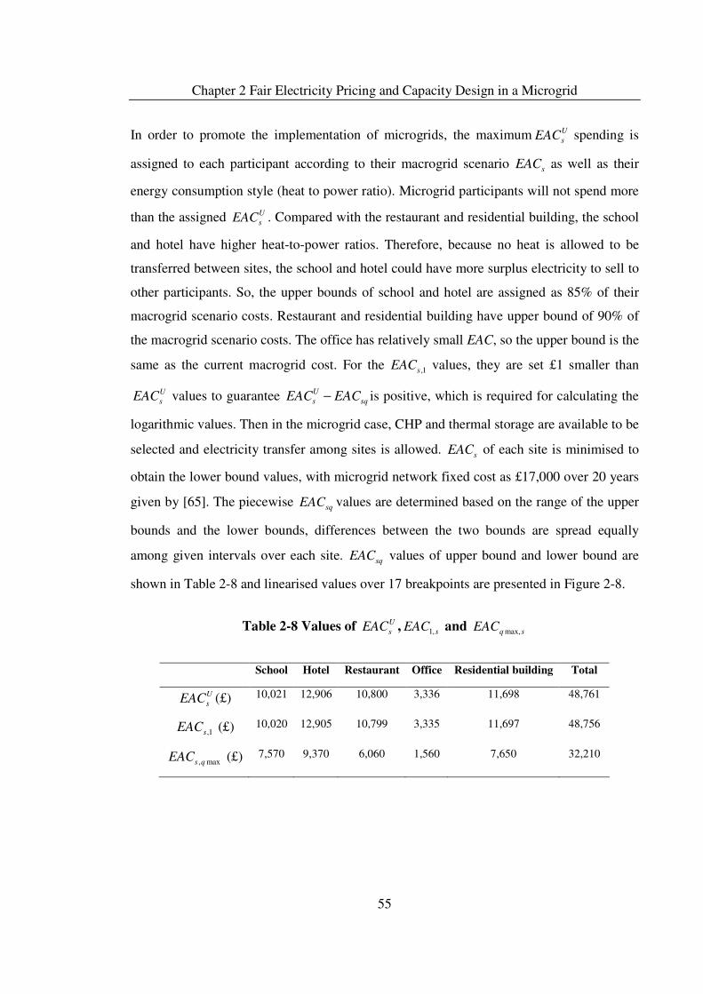
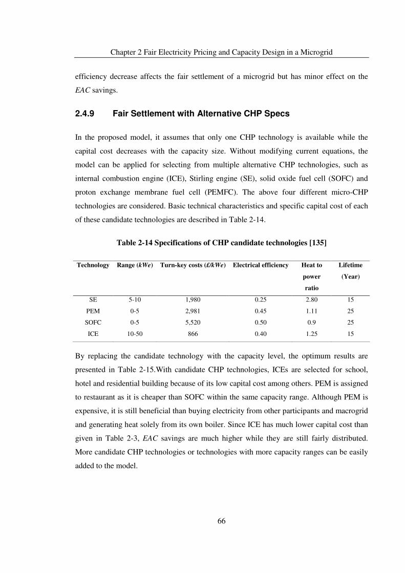
2.4 CASE STUDY ...................................................................................................................................45 2.4.1 Basic Technical Parameters and Costs of Microgrid Candidate Technologies........................46 2.4.2 Energy Demand Profiles ...........................................................................................................47 2.4.3 Global Microgrid EAC Savings with Gas Price, Electricity Buying and Selling Prices...........50 2.4.4 EAC Upper Bounds ...................................................................................................................54 2.4.5 Global Minimum Microgrid EAC..............................................................................................56 2.4.6 Application of Game Theory for Fair Settlement ......................................................................58 2.4.7 Fair Settlement under Peak Demand Charge............................................................................62 2.4.8 Fair Settlement with lower CHP overall efficiency...................................................................65 2.4.9 Fair Settlement with Alternative CHP Specs.............................................................................66

2.5 CONCLUSIONS.................................................................................................................................67

CHAPTER 3 OPTIMAL ENERGY CONSUMPTION SCHEDULING AND OPERATION MANAGEMENT OF SMART HOMES MICROGRID .............................................................................69

3.1 INTRODUCTION AND LITERATURE REVIEW .....................................................................................69 3.1.1 Operation Planning in Microgrid .............................................................................................69 3.1.2 Energy Consumption in Smart Buildings ..................................................................................71

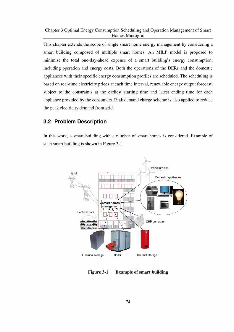
3.2 PROBLEM DESCRIPTION ..................................................................................................................74 3.3 MATHEMATICAL FORMULATION.....................................................................................................77

6

3.3.1 Nomenclature ............................................................................................................................77 3.3.2 Capacity Constraints.................................................................................................................80 3.3.3 Energy Storage Constraints ......................................................................................................81 3.3.4 Wind Generator Output.............................................................................................................82 3.3.5 Energy Balances........................................................................................................................83 3.3.6 Starting Time and Finishing Time.............................................................................................83 3.3.7 Peak Demand Charge ...............................................................................................................84 3.3.8 Objective Function ....................................................................................................................84

3.4 ILLUSTRATIVE EXAMPLES...............................................................................................................86 3.4.1 Example 1: Smart Building of 30 Homes with Same Living Habits ..........................................86 3.4.2 Example 2: Smart Building of 90 Homes with Different Living Habits ....................................89

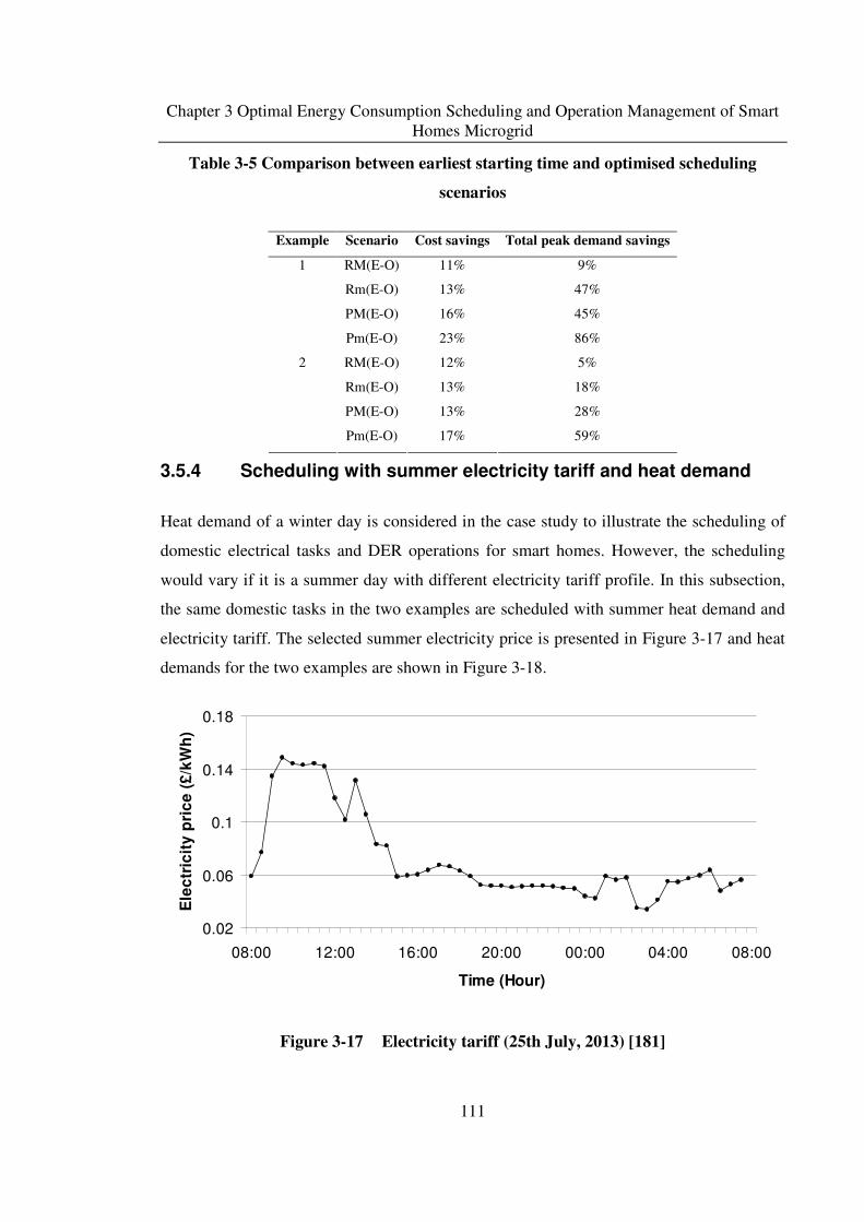
3.5 COMPUTATIONAL RESULTS.............................................................................................................90 3.5.1 Example 1:Real-Time Price and Peak Demand Price Schemes................................................92 3.5.2 Example 2:Real-Time Price and Peak Demand Price Schemes..............................................101 3.5.3 Comparison between Example 1 and Example 2 ....................................................................110 3.5.4 Scheduling with summer electricity tariff and heat demand....................................................111 3.5.5 Scheduling with wider time window ........................................................................................114

3.6 CONCLUDING REMARKS ...............................................................................................................116

CHAPTER 4 COST DISTRIBUTION AMONG MULTIPLE SMART HOMES.............................118

4.1 INTRODUCTION AND LITERATURE REVIEW ...................................................................................118 4.2 PROBLEM DESCRIPTION ................................................................................................................120 4.3 MATHEMATICAL FORMULATION...................................................................................................121

4.3.1 Nomenclature ..........................................................................................................................121 4.3.2 Capacity Constraint ................................................................................................................123 4.3.3 Energy Storage Constraints ....................................................................................................124 4.3.4 Energy Balances......................................................................................................................127 4.3.5 Starting Time and Finishing time ............................................................................................127 4.3.6 Daily Cost................................................................................................................................128

4.4 LEXICOGRAPHIC MINIMAX APPROACH TO FIND A FAIR SOLUTION...............................................128 4.5 ILLUSTRATIVE EXAMPLES.............................................................................................................131

4.5.1 Example 1: 10 Smart Homes ...................................................................................................131 4.5.2 Example 2: 50 Smart Homes with Different Types of Household ...........................................136

4.6 COMPUTATIONAL RESULTS...........................................................................................................137 4.6.1 Computational Environment ...................................................................................................138 4.6.2 Example 1 Results ...................................................................................................................138 4.6.3 Example 2 Results ...................................................................................................................142


CHAPTER 5 OPTIMAL SCHEDULING OF ELECTRIC VEHICLE BATTERY USAGE WITH DEGRADATION ..........................................................................................................................................146

5.1 INTRODUCTION AND LITERATURE REVIEW ...................................................................................146 5.2 PROBLEM DESCRIPTION ................................................................................................................149 5.3 MATHEMATICAL FORMULATION...................................................................................................150

5.3.1 Nomenclature ..........................................................................................................................150 5.3.2 Charge and Discharge Constraints.........................................................................................152 5.3.3 EV Battery Storage Constraints ..............................................................................................153 5.3.4 Electricity Demand Constraints ..............................................................................................153 5.3.5 SOC Constraints......................................................................................................................154 5.3.6 Electricity Demand Threshold Constraints .............................................................................155 5.3.7 Degradation Cost Constraints.................................................................................................155 5.3.8 Objective Function ..................................................................................................................155

5.4 CASE STUDY .................................................................................................................................156 5.5 COMPUTATIONAL RESULTS...........................................................................................................161

5.5.1 Business-as-Usual Results.......................................................................................................161 5.5.2 Optimal Results without Degradation Costs ...........................................................................162

7

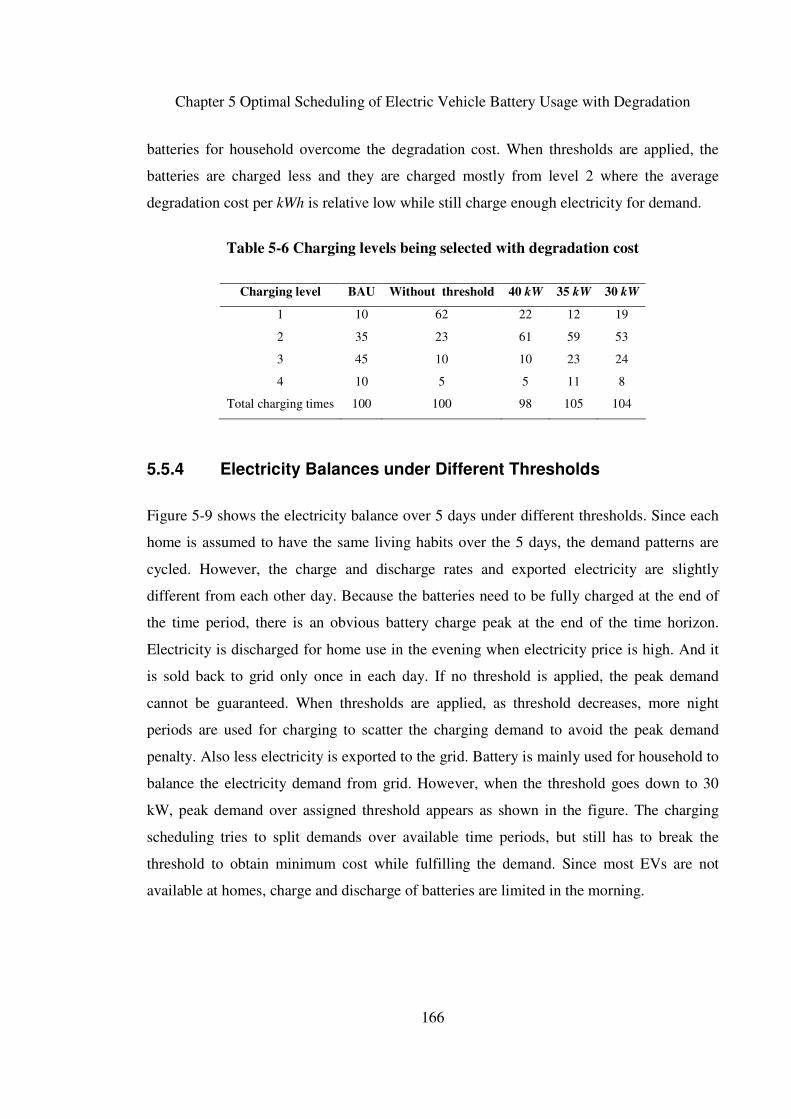
5.5.3 Optimal Results with Degradation Costs ................................................................................163 5.5.4 Electricity Balances under Different Thresholds ....................................................................166


CHAPTER 6 CONCLUSIONS AND FUTURE WORK ......................................................................171

6.1 CONTRIBUTIONS OF THIS THESIS ..................................................................................................171 6.2 FUTURE WORK .............................................................................................................................172

APPENDIX A PARAMETERS OF CHAPTER 2......................................................................................175

APPENDIX B PARAMETERS OF CHAPTER 3......................................................................................180

APPENDIX C PARAMETERS OF CHAPTER 4......................................................................................186

APPENDIX D PARAMETERS OF CHAPTER 5......................................................................................196

APPENDIX E PUBLICATIONS .................................................................................................................200

REFERENCES..............................................................................................................................................201

8

List of Figures

Figure 1-1 Microgrid example [5] ................................................................................. 12 Figure 1-2 Microgrid key components .......................................................................... 16 Figure 2-1 Participants of a microgrid ........................................................................... 29 Figure 2-2 Electricity demand (winter day) [131] ......................................................... 49 Figure 2-3 Heat demand (winter day) [131] .................................................................. 49 Figure 2-4 EAC savings as a function of gas, electricity buying and selling prices...... 51 Figure 2-5 EAC savings as a function of gas and electricity selling prices to grid ....... 52 Figure 2-6 EAC savings as a function of electricity buying and selling prices............. 53 Figure 2-7 EAC savings as a function of gas and electricity buying prices .................. 54 Figure 2-8 sqEAC linearised values............................................................................... 56

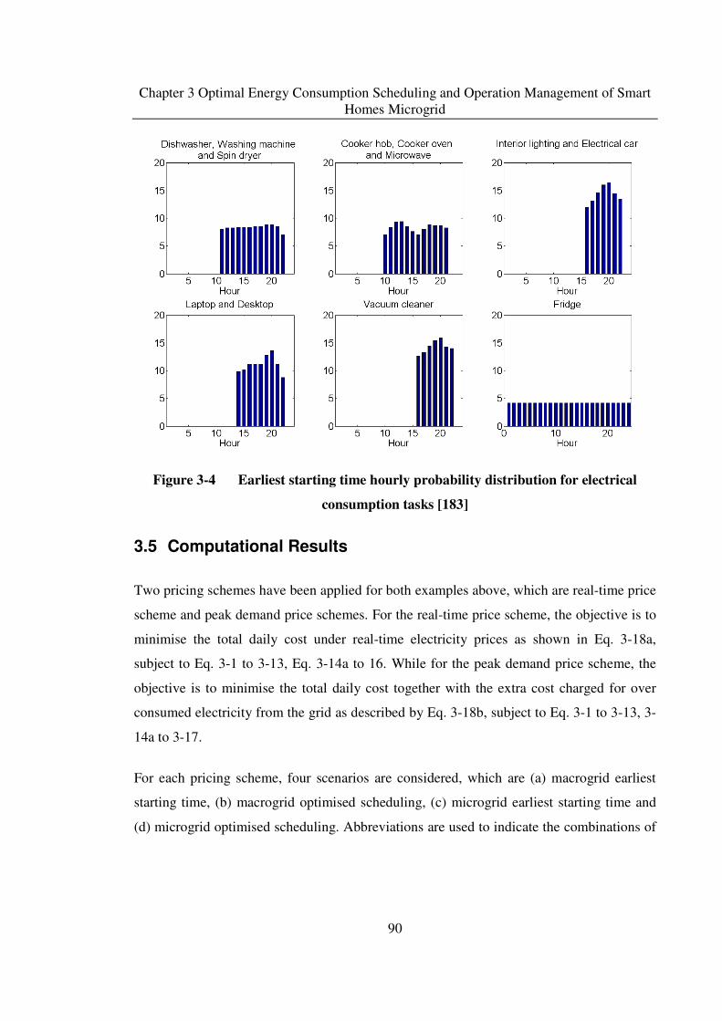
Figure 2-9 EAC savings of each microgrid participant without Game theory .............. 57 Figure 2-10 EAC values of each microgrid participant ................................................... 59 Figure 2-11 Contributions to microgrid electricity demand ............................................ 61 Figure 2-12 Contributions to microgrid electricity demand under heat dumping ........... 62 Figure 2-13 Grid electricity supply under macrogrid and microgrid case under peak demand charge ..................................................................................................................... 64 Figure 3-1 Example of smart building........................................................................... 74 Figure 3-2 Electricity tariff (3rd March, 2011) [181] .................................................... 87 Figure 3-3 Electricity utilisation profiles of dishwasher and washing machine............ 88 Figure 3-4 Earliest starting time hourly probability distribution for electrical consumption tasks [183] ...................................................................................................... 90 Figure 3-5 30 homes: Macrogrid electricity balance and total cost under real-time price scheme ...................................................................................................................... 93 Figure 3-6 30 homes: Microgrid electricity balance and total cost under real-time price scheme ...................................................................................................................... 94 Figure 3-7 30 homes: Macrogrid electricity balance and total cost under peak demand price scheme ...................................................................................................................... 96 Figure 3-8 30 homes: Microgrid electricity balance and total cost under peak demand price scheme ...................................................................................................................... 97 Figure 3-9 30 homes: heat balance for microgrid real-time price scenarios.................. 99 Figure 3-10 30 homes: heat balance for microgrid peak demand price scenarios......... 100 Figure 3-11 90 homes: Macrogrid electricity balance and total cost under real-time price scheme .................................................................................................................... 102 Figure 3-12 90 homes: Microgrid electricity balance and total cost under real-time price scheme .................................................................................................................... 103 Figure 3-13 90 homes: Macrogrid electricity balance and total cost under peak demand price scheme .................................................................................................................... 105 Figure 3-14 90 homes: Microgrid electricity balance and total cost under peak demand price scheme .................................................................................................................... 106 Figure 3-15 90 homes: heat balance for microgrid real-time price scenarios................ 108 Figure 3-16 90 homes: heat balance for microgrid peak demand price scenarios......... 109 Figure 3-17 Electricity tariff (25th July, 2013) [181] .................................................... 111 Figure 3-18 Heat demands of 30 and 90 homes in a summer day [182] ....................... 112

9

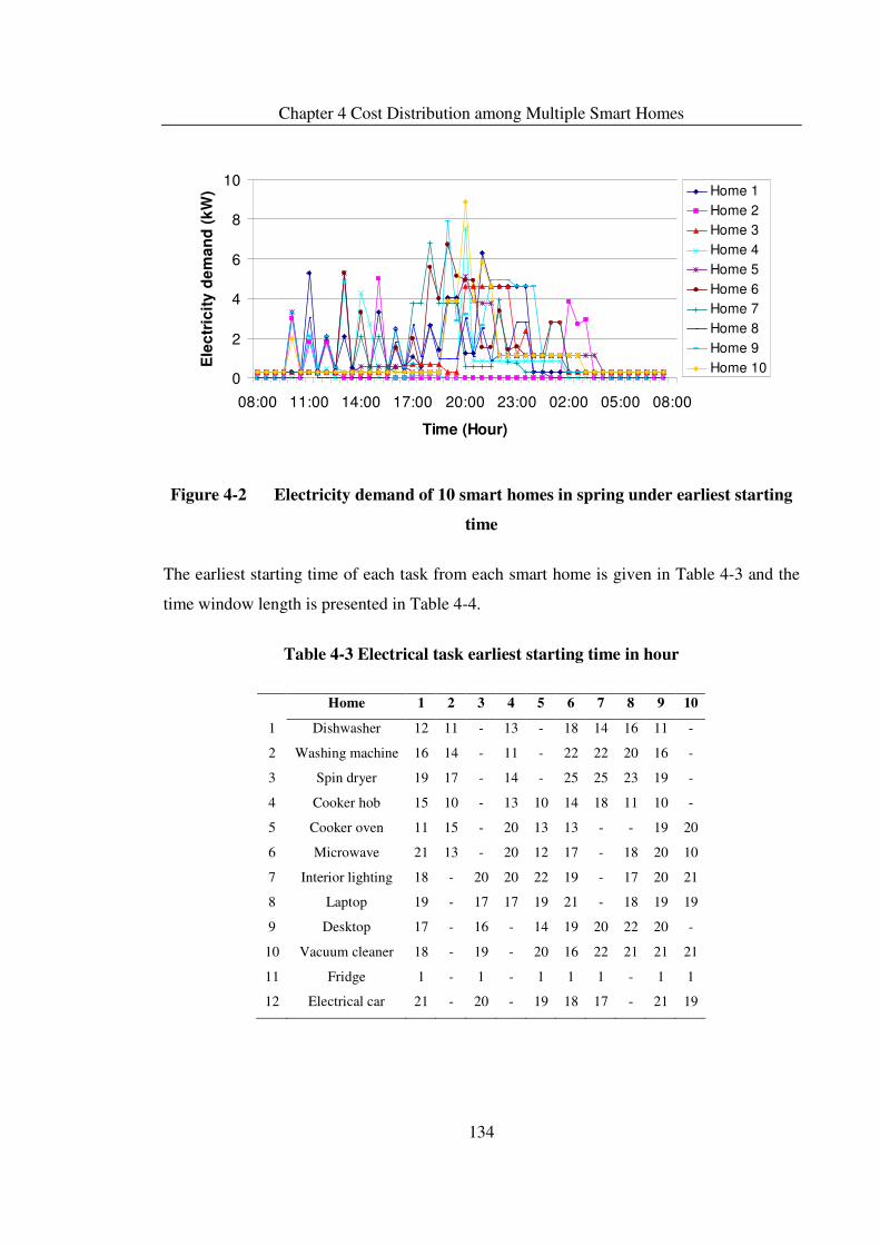
Figure 4-1 Heat demands of 10 smart homes in spring ............................................... 132 Figure 4-2 Electricity demand of 10 smart homes in spring under earliest starting time.. .................................................................................................................... 134 Figure 4-3 Total energy demand of 10 smart homes in spring under earliest starting time .................................................................................................................... 135 Figure 4-4 Heat demands of typical homes in winter .................................................. 136 Figure 4-5 Total energy demand of 50 smart homes in winter under earliest starting time .................................................................................................................... 137 Figure 4-6 Optimal electricity demands of Example 1................................................ 140 Figure 4-7 Electricity balance of Example 1 under fairness concern .......................... 141 Figure 4-8 Heat balance of Example 1 under fairness concern ................................... 142 Figure 4-9 Electricity balance of Example 2 under fairness concern .......................... 144 Figure 4-10 Heat balance of Example 2 under fairness concern ................................... 144 Figure 5-1 EV daily travel demand.............................................................................. 156 Figure 5-2 Number of occurrence of EV arriving ....................................................... 157 Figure 5-3 Number of EVs staying at home ................................................................ 158 Figure 5-4 Unrestricted domestic electricity demand for winter weekday [227] ........ 159 Figure 5-5 Electricity tariff (March 3rd , 2011) [181] ................................................. 159 Figure 5-6 Normalised cost of cycling a battery to a given depth of discharge with a $750 capital cost [193] ....................................................................................................... 160 Figure 5-7 Degradation cost associated with the electricity charged .......................... 161 Figure 5-8 Electricity balance under BAU scenario .................................................... 162 Figure 5-9 Optimum 5-day electricity balances........................................................... 167 Figure 5-10 Optimum Day 1 electricity balances .......................................................... 169

10

List of Tables

Table 2-1 Description of sEAC components ....................................................................... 38

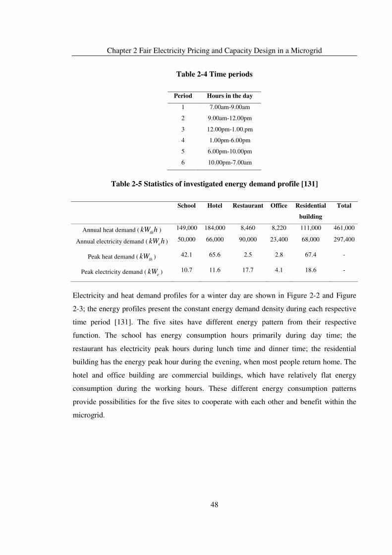
Table 2-2 Technical parameters and costs of microgrid candidate technologies [65]......... 46 Table 2-3 CHP turn-key cost and electrical efficiency [131, 132] ...................................... 47 Table 2-4 Time periods ........................................................................................................ 48 Table 2-5 Statistics of investigated energy demand profile [131] ....................................... 48 Table 2-6 Model summaries................................................................................................. 50 Table 2-7 Optimal results of macrogrid scenario................................................................. 54 Table 2-8 Values of U

sEAC , sEAC ,1 and sqEAC max, ............................................................. 55

Table 2-9 Optimum EAC results without Game theory....................................................... 57 Table 2-10 Optimum results with Game theory................................................................... 59 Table 2-11 Transfer price between sites and annual transferred amount............................. 60 Table 2-12 Peak demand charge scheme with game theory ................................................ 63 Table 2-13 Optimal design with 80% CHP overall efficiency ............................................ 65 Table 2-14 Specifications of CHP candidate technologies [135] ........................................ 66 Table 2-15 Optimal design with candidate CHP technologies ............................................ 67 Table 3-1 Electricity consumption for different electrical tasks [179] ................................ 76 Table 3-2 Model statistics .................................................................................................... 92 Table 3-3 Results of Example 1 under two pricing schemes ............................................... 98 Table 3-4 Results of Example 2 under two pricing scheme............................................... 107 Table 3-5 Comparison between earliest starting time and optimised scheduling scenarios............................................................................................................................................ 111 Table 3-6 Results of Example 1 under summer electricity tariff and heat demand ........... 113 Table 3-7 Results of Example 2 under summer electricity tariff and heat demand ........... 113 Table 3-8 Comparison between earliest starting time and optimised scheduling scenarios with summer electricity tariff and heat demand................................................................. 114 Table 3-9 Results of Example 1 with 2 hours wider time window.................................... 115 Table 3-10 Results of Example 2 with 2 hours wider time window.................................. 115 Table 3-11 Comparison between earliest starting time and optimised scheduling scenarios with 2 hours wider time window........................................................................................ 116 Table 4-1 Household occupancy types [192]..................................................................... 132 Table 4-2 Electrical task of each smart home .................................................................... 133 Table 4-3 Electrical task earliest starting time in hour ...................................................... 134 Table 4-4 Electrical task time window length in hour ....................................................... 135 Table 4-5 Detail types of household .................................................................................. 137 Table 4-6 Model statistics .................................................................................................. 138 Table 4-7 Cost of each home from minimising total cost and fairness concern ................ 139 Table 4-8 Optimal results of Example 2 ............................................................................ 143 Table 5-1 Battery cycle cost from different SOC .............................................................. 154 Table 5-2 Nissan Leaf battery pack specification [226] .................................................... 156 Table 5-3 Optimal results under different thresholds without degradation cost................ 163 Table 5-4 Optimal results under different thresholds with degradation cost ..................... 164 Table 5-5 Charging levels being selected without degradation cost.................................. 165 Table 5-6 Charging levels being selected with degradation cost ....................................... 166

Chapter 1 Introduction


Current energy system is dominated by centralised generation, with electricity distributed to

users through a macrogrid. Due to energy demand increase and the rise of global emissions

of greenhouse gases, the current centralised energy generation system is challenged and

needs to be restructured to meet the world’s growing electricity needs [1]. Microgrids are

emerging as an integral feature of the future power systems and are considered as a

promising alternative to centralised generation. As a localised energy providing system,

problems arise along with the processes of design and utilisation. This thesis aims to

address some key problems in the optimal design and operation planning of microgrid

through mathematical programming techniques.

1.1 Microgrid

Microgrid is a relatively small-scale localised energy network, which includes loads,

network control system and a set of distributed energy resources (DER), such as generators

and energy storage devices. A microgrid equipped with intelligent elements from smart

grids has been adopted to enable the widespread of DERs and demand response programs

in distribution systems [2], which is considered as future smart grid. Microgrids can be

applied for single consumer, such as sport stadium; community microgrid with multiple

consumers, such as campus; and utility microgrid with supply resources on utility side with

consumer interaction and utility objectives [3]. Remote off-grid systems and military

microgrids are also mentioned in [4]. In this thesis, the community microgrid is addressed.

Figure 1-1 shows a microgrid example for application at community level [5]; it has a

group of consumers, including residential buildings, factories and commercial building

which have their own energy loads. The local DERs are a wind generator, photovoltaic

(PV) panels and other generators to provide local electricity and energy storage systems for

energy storage. There is also macrogrid utility connection to buy electricity when there is

not enough electricity generated from local generators or to sell electricity back when there

is excess electricity generated. When there is an emergency, the macrogrid can be


12

disconnected and the microgrid can work independently to provide electricity in the

‘islanded’ mode.

Figure 1-1 Microgrid example [5]

Microgrids have been developed for a number of reasons: they can provide better power

quality and reliability in case of blackout or other problems on the external network and

they also support voltage and reduce voltage dips [6]. They may have economic and

environmental benefits when emissions credits are considered because they can utilise more

low carbon energy sources such as wind and solar energy; and they are localised which

implies some transmission infrastructure and associated costs may be avoided.

Additionally, primary energy consumption could be reduced when combined heat and

power (CHP) technology is applied [7]. Moreover, microgrids could support the macrogrid

handling sensitive loads from DERs locally and integrate them for peak power consumption

time which alleviate or postpone current macrogrid upgrades and also reduce the central

generation reserve requirements [8, 9]. The microgrid can be designed according to


13

customer’s respective interests, such as enhancing local reliability, reducing feeder losses

and uninterruptable power supply [10]. The microgrid is also one solution for energy

generation in remote areas without electricity service. Finally, microgrids also have the

inherent advantages of being interconnected via a local or private network, so the

participants can cooperate with each other thus increasing equipment utilisation and

providing yet more benefits.

1.1.1 Microgrid Concept

The microgrid concept has been popular and researched by many experts, especially in

U.S., E.U., Canada and Japan [8, 11]. It operates and fulfils the local energy demands

according to its own protocols and standards [12, 13]. However, the concepts proposed vary

and there is still no common concept for microgrids [14-18]. The U.S. Consortium for

Electric Reliability Technology Solutions (CERTS) has published a White Book [19] where

a microgrid is defined as follows:

“The Consortium for Electric Reliability Technology Solutions (CERTS)

MicroGrid concept assumes an aggregation of loads and microsources

operating as a single system providing both power and heat. The majority of

the microsources must be power electronic based to provide the required

flexibility to insure operation as a single aggregated system. This control

flexibility allows the CERTS MicroGrid to present itself to the bulk power

system as a single controlled unit that meets local needs for reliability and

security.”

While the U.S. Department of Energy (DOE) [20] defines microgrids as:

“a group of interconnected loads and distributed energy resources (DER) with

clearly defined electrical boundaries that acts as a single controllable entity

with respect to the grid and can connect and disconnect from the grid to enable

it to operate in both grid-connected or island mode.”


14

For the researchers apart from U.S., other aspects of microgrid are considered, Abu-Sharkh

et al. [21] describes microgrid simply as:

“a small-scale power supply network that is designed to provide power for a

small community.”

In the definition provided by Hatziargyriou et al. [8]:

“Microgrids are defined as low voltage or in some cases, e.g. Japan, as medium

voltage networks with distributed generation sources, together with storage

devices and controllable loads (e.g. water heaters, air conditioning) with total

installed capacity in the range of few kWs to couple of MWs.”

Zhang et al. [22] define microgrid as:

“a cluster of loads and relatively small energy sources operating as a single

controllable power network to supply the local energy needs.”

Also Funabashi and Yokoyama [23] describe it as:

“Microgrid is a small grid in which distributed generations and electric loads

are placed together and controlled efficiently in an integrated manner. It

contributes to utility grid’s load levelling by controlling power flow between

utility grid and Microgrid according to predetermined power flow pattern. Also,

it contributes to an efficient operation of distributed generations by operation

planning considering grid economics and energy efficiency.”

1.1.2 Microgrid Key Components

Microgrids usually consist of distributed energy resources, power conversion equipment,

communication system, controllers and energy management system to obtain flexible

energy management [24, 25]. The customer is another key component for microgrid to be

promoted and implemented [21].


15

• DER involves distributed generator (DG) and distributed storage and provides

energy to meet energy demand.

• Controllers are necessary for microgrid to apply demands to DERs and control their

parameters, such as frequency, voltage and power quality [26].

• Power conversion equipment, such as voltage and current transformer, are utilised

to detect the microgrid running state. Also, the DERs produce DC or AC voltage

with different amplitude and frequency than grid, power electric converter interface

is necessary [27].

• Communication system is a medium to convey monitoring and control information

in microgrids. It is applied to interconnect different elements within the system and

ensures management and control [28, 29].

• Energy management system is used for data gathering and device control, state

estimate and reliability evaluation of the power system [30]. It also functions in

power prediction from renewable energy, load forecasting and power planning [31].

Major vendors for energy management system are summarised by [32].

• Customers, who may also be the suppliers, will affect technique selection, load

control and operation of microgrid from cost and efficiency concerns. Microgrid can

be deployed in demand response driven by customers [33]. The participation of

customers is the fundamental driver for smart grid [34] and strongly encourage the

engagement desired from the developers [35]. The customers function in user

interaction needs, behaviour change, community initiatives and resources

management [36].

Figure 1-2 illustrates the key components of microgrid, the solid line represents the

communication system information transfer.


16

Figure 1-2 Microgrid key components

1.1.3 Microgrid and DER

A microgrid consists of a variety of distributed energy resources, such as generators, energy

storage and energy demand itself. The capacity of the DER considered in microgrid is in

relatively small scale, but without universal agreement. It is mentioned as smaller than 100

kW by Huang et al. [37], and in [38] micro-generation is considered with even smaller

scale, less than 3 kW electrical and 30 kW thermal while standard EU definition of micro-

generation being up to 50 kW based on different residential scales. While authors of [39]

consider it smaller than 500 kW. Generally, the generators have a similar capacity size as

the loads within the microgrid, and they are located close to the end users [21].

The distributed generators applicable for a microgrid comprise emerging technologies, such

as CHP, wind generators, photovoltaic arrays, and also some well established generators,

such as synchronous generators driven by internal combustion engines or small hydro [17,

24, 40]. The advantage of high energy efficiency of CHP results from energy cogeneration.

Fossil fuel power sources CHP for microgrid are summarised in [21] and [41], which are

internal combustion engine, micro-turbine, sterling engine and fuel cell.

Due to the small generators usually used, a microgrid is not able to respond to sudden load

changes or disturbances rapidly. So, energy storage devices are essential for microgrid,

especially under the circumstances when intermittent generators and included, limited


17

methods of energy generation are available or the microgrid works under islanded mode.

Electrical storage devices have several forms, including gravitational potential energy with

water reservoirs, batteries and flow batteries, super-capacitors, flywheels, superconducting

magnetic energy storage, compressed air energy storage, fuel cell and thermal energy

storage and use of traditional generation with inertia [42-44]. Among the available energy

storage technologies, batteries, fly-wheels and super-capacitors are particularly suitable for

microgrids [37].

Because of the characteristics of energy produced by renewable energy, the use of

microgrid to integrate DERs can obtain the optimal benefit. Especially when different types

of generators are available, they can compensate with each other while energy storage

provides energy stability and quality [45] which enable higher penetration of many types of

distributed generators [46]. Energy storage systems are also desirable to reshape the peak

demand and store energy at the time of surplus and reused later [47].

1.1.4 Existing Microgrids

Microgrids have been studied worldwide and testing systems have been established for

research. In the U.S., the CERTS testbed has been built near Columbus, Ohio and a battery

storage is also available. University of Wisconsin-Madison has an UW microgrid testbed

with a diesel driven generator [48]. There is a Smart Polygeneration Microgrid test-bed

facility in the Genoa University and it is located at Savona Campus teaching & research

facilities [49]. While in Canada, BC Hydro Boston Bar microgrid supplies power without

energy storage unit and Hydro Quebec Senneterre substation systems serves 3000

customers with islanding attempt in 2005 [50]. In Europe, Bronsbergen Holiday Park with

208 holiday homes in Netherland has a microgrid to provide electricity from 108 roof fitted

solar PVs and energy storage is also available as two battery banks [51]. A residential Am

Steinweg microgrid is built in Stutensee in German, and it is a test system with CHP and

PV as generators and a lead acid battery bank for energy storage. Another microgrid system

in German is DeMoTec test microgrid, which has two diesel gensets, a PV generator and a

wind generator and two battery units are also included [52] Italy has a CESI RICERCA

DER test microgrid equipped with a fly wheel and battery banks. The Kythnos islanded


18

microgrid in Greece provides electricity for 12 houses with PVs, diesel generator set and

battery bank while the laboratory-scale microgrid system at National Technical University

of Athens consisting of two PV generators, one wind turbine and battery for energy storage

[52, 53]. In the UK, University of Manchester has a laboratory microgrid with a

synchronous generator and an induction motor coupled together as micro-source and a

flywheel as energy storage [54]. Microgrid projects are more popular in Japan, under

Energy and Industrial Technology Development Organisation (NEDO), Aichi microgrid,

Kyoto eco-energy project and Hachinohe project are established. Fuel cells, PV and

sodium-sulfur (NaS) battery are equipped in the Aichi microgrid [55]. Kyoto eco-energy

microgrid has gas engines, a molten carbonate fuel-cell (MCFC), two PV systems, a wind

turbine and lead-acid battery [56]. The Hachinohe microgrid includes a gas engine, several

PV systems, a wind farm and a battery storage. A test network is located at Akagi of the

Central Research Institute of Electric Power Industry, and no energy storage is included

[57]. One more microgrid from Japan is the Sendai microgrid with two gas engine

generators, one MCFC, PV and battery storage [58]. For China, there are a testbed

microgrid in Hefei University of Technology [59] and a demonstrative microgrid

implemented in Caoxi implemented by Grid Corporation of Shanghai [25]. A microgrid

pilot plant has been constructed in Korea Electro-technology Research Institute and it

includes PV, PV and wind hybrid, two diesel generators and battery energy storage system

[60].

1.2 Optimal Design and Planning for Microgrids

Studies on microgrids are generally classified into two groups: system design and operation

planning[61]. They are critical for the successful realisation of microgrid in real-time

applications [62]. System design is a long-term planning activity of microgrids, which

involves the selection and sizing of DERs with the objective of minimum cost,

environmental or energy security issues [63]. The design of DERs plays an important role

in order to maintain the reliability of the power grid, level of short-circuit current, power

flow and node voltage [64]. The selection technique is constrained by energy loads,

technology information, operation and maintenance cost, utility tariff from different tariff

schemes and weather conditions. The optimal capacity sizing tradeoffs between peak loads


19

satisfaction and investment costs minimisation. Since energy demand fluctuates due to

uncertainty in human behaviours and ambient conditions, hourly energy demand profile

representing the dynamic nature of the problem is commonly applied to the design of

microgrids [65, 66].

On the other hand, with given DER capacity operation planning deals with optimal

microgrid planning over the short term, such as a day or week; and the time interval can be

one hour or even smaller. Microgrid planning includes the overall management of a

microgrid. It targets at obtaining an economically attractive performance under uncertainty

and disturbances due to the variability of renewable energy sources and the rapid change in

the power/heat demand. The optimal operation of microgrid includes two main functions,

supply side optimisation and demand side optimisation. For the supply side, energy

management decisions include the DER operations (production output, switch on/off status

or types of fuel) and electricity purchases or sales back to grid [67]. Generation scheduling

is defined as the scheduling of power production from generation units over certain time

horizon while satisfying technology and system constraints [68]. DER operation generation

schedule results in the cost savings under operational constraints of each DER over given

time periods [30]. Demand side management involves controlling the condition of the

energy system through demand modification, changing the shape of the load and optimising

the generation, delivery and end use processes[69, 70]. At the same time, demand side

management aggregates all energy-consuming devices and flexible loads can be

rescheduled. Demand side management benefits in peak reduction, load profile reshape and

overall cost and emission reductions.

1.3 Smart Grids and Microgrids

The ageing current electricity power infrastructure needs to be upgraded or transformed for

environmental concerns, energy conservation as well as to accommodate increasing energy

demands. Future electricity distribution system will be integrated, intelligent and better

known as smart grids, which include advanced digital meters, distribution automation,

communication systems and DERs. Central distributed and intermittent sources will all be

included [71]. Desired smart grid functionalities include self-healing, optimising asset


20

utilisation and minimising operations and maintenance expenses [72]. In addition, a smart

grid needs to be dynamic and has constant bi-communication involving consumers’ own

decision on how to use energy [73]. Many national and international projects address the

smart grid concept, although there is still no agreed universal concept about it [74, 75].

Bracco et al. [49] present an overview of the smart grid projects around the world.

In a smart grid, bidirectional communication between the grid and consumers is available

for energy flow where smart meters and sensors are utilised [35, 76]. With the application

of energy management and two-way communication functions, energy consumption load

can be reshaped. There is possibility to shift the energy generation from peak demand base

to real-time demand need base [77]. Residential end-users will also play a more active role

as a co-provider rather than a passive role in balancing supply and demand [36].

Microgrid has various smart grid initiatives and is expected to be prototype for smart grid

because of its experimentation scalability and flexibility [2]. The small scale of microgrid

provides the convenience to adopt new technologies [78]. As a significant ingredient of the

future smart grid, microgrid is considered to enable widespread inclusion of renewable

resources, distributed storage and demand response programs in distribution [2]. Also, with

the help of Information and Communication Technologies (ICT), smart microgrids can be

connected to form a network to work collaboratively for the reliability and sustainability of

electrical services [79]. In [80], smart grid is referred to as a network of integrated

microgrids that can monitor and heal itself. Smart grids composing of several microgrids

are classified in [81].

1.4 Aim and Scope of This Thesis

A microgrid equipped with intelligent elements from smart grids has been adopted and

active control of small scale energy resources is included in such smart microgrid. Such

control has benefited from research attention in technical aspects [14-16], however, limited

studies are available for exploring the economic incentive of participants to become

involved in a microgrid. Therefore, this thesis aims at addressing this gap by considering

the consumer engagement and their interaction. The aim of this work is to develop


21

frameworks based on mathematical programming techniques in order to integrate request

from individual customer into the optimal design and planning of microgrid.

The issues covered in this thesis and contributions of this work are: firstly, a fair economic

settlement scheme for participants in a microgrid is proposed. Electricity transfer price and

unit capacity selection are obtained under given customer energy demands and their

accepted equivalent annual cost upper bounds. Then, efficient energy consumption and

operation management of a smart building with microgrid is addressed, where customers

provide their energy consumption tasks and flexible time windows to minimise their total

energy cost and reduce the peak demand from grid. Thirdly, problem of fair cost

distribution among multiple smart homes sharing common microgrid is considered. Each

customer competes with other neighbours to obtain lowest energy bill under accepted cost

limits. Finally, as a special electricity consumption task in a smart home, electric vehicle

battery operation is considered. It is scheduled based on customer’s living habit, such as

travelling time and respective home energy demand, to optimise the battery usage while

considering the degradation effects.

1.5 Outline of the Thesis

The rest of the thesis is divided in five chapters:

In Chapter 2, the problem of fair electricity transfer price and unit capacity selection for

microgrid is addressed. A mixed integer non-linear programming (MINLP) model is

proposed based on the Game-theory Nash bargaining solution approach. Then a separable

programming approach is applied to reform the resulting mixed integer non-linear

programming model as a mixed integer linear programming (MILP) model.

In Chapter 3, the optimal scheduling of smart homes’ energy consumption is studied using

an MILP approach. In order to minimise a one-day forecasted energy consumption cost,

DER operation and electricity-consumption household tasks are scheduled based on real-

time electricity pricing, electricity task time windows and forecasted renewable energy

output.


22

In Chapter 4, a mathematical model is proposed for the fair cost distribution among smart

homes with microgrid, which is based on the Lexicographic minimax method using an

MILP approach. It schedules DER operation, DER output sharing among smart homes and

electricity consumption household tasks.

In Chapter 5, the intensive use of battery in household and vehicle to grid (V2G)

applications is studied while an MILP model is proposed to provide the charging

scheduling for load shifting and cost minimisation together with minimising degradation

cost. Two boundaries for demand from grid are applied to guarantee the stability of the

grids.

Finally, Chapter 6 summarises the main contributions of the thesis and provides

recommendations for future work.

Chapter 2 Fair Electricity Pricing and Capacity Design in a Microgrid

23


As a localised energy network, microgrids are proposed to alleviate current macrogrid

demand burden and reduce emissions. The successful deployment of microgrids depends

heavily upon the DERs combination selection, capacity sizing and operation plan.

Microgrids can be considered as collaborative networks and cooperation amongst microgrid

participants can provide better economic outcome than being isolated from each other with

pure self interest. The participants in a microgrid can benefit from cooperation for

improved design and operation. Although a number of models have been developed for cost

minimisation of the whole microgrid, the cost to respective participants is usually not

considered.

In this chapter, an MILP model that optimises the respective cost distribution amongst

participants in a microgrid is proposed based on the game theoretical Nash method.

2.1 Introduction and Literature Review

A number of concepts have emerged in recent years in relation to deployment and control

of DERs, such as smart grids and microgrids. These concepts represent a significant

departure from the top-down and asset-intensive nature of current electricity systems, and

capitalise on the availability of new generation equipment and ICT systems to facilitate the

use of many small-scale energy resources to serve growing demands. Such technology can

provide economic benefits through avoidance of investment as demonstrated in upstream

infrastructure, security and reliability benefits through interconnection and coordinated

control, and environmental (and additional economic) benefits by using low carbon/low

pollutant generation and co-production of heat and power. The smart grid concept remains

only loosely defined at present based on specific focuses [74, 75]. However, active control

of small scale energy resources is most likely to be included. This work addresses the

economic incentive of customers by considering a fair economic settlement scheme for

participants in a microgrid.


24

2.1.1 Unit Capacity Selection in Microgrids

Several studies have considered how to design the capacity of a microgrid system to

minimise the annual cost of meeting demand [7, 82, 83]. A computer program that

optimises the equipment arrangement of each building linked to a fuel cell network and the

path of the hot-water piping network under the cost minimisation objective has also been

developed [84]. Another work considering the optimal DER sizing and allocation problem

is given by [85]. Kumar et al. [86] propose an architecture of smart microgrid for

integration of renewable energy sources, and it focuses on the design, modelling and

operational analyses. Optimal plan and design of DER capacity in microgrid is also

provided by [87] based on the Chinese meteorological conditions, the authors also present

the allocation method of output power. Authors of [88] propose a generalised approach to

design generation capacity sizing and power quality evaluation for a microgrid in islanded

and grid connected modes, where PSCAD (Power System Computer Aided Design)

software is used for modelling. And in [89] generation design is addressed in islanded

mode along with the analysis of power reliability and voltage quality of the system. The

optimal configuration of DGs at different locations is obtained by applying

electromagnetism-like mechanism in [64]. Mizani and Yazdani [90] demonstrate the

optimal selection of DER in a grid connected microgrid together with optimal dispatch

strategies and they can reduce microgrid lifetime cost and emission on a campus. Proper

CHP-based DERs are deployed in the work of [91] and optimisation is done using particle

swarm optimisation (PSO) technique. Bando et al. [92] develop a methodology for the

designing of DER in microgrid with steam supply from a municipal waste incinerator, and

both primary energy consumption and CO2 emissions have been reduced. A genetic

algorithm (GA)-based optimal design of microgrid is investigated under pool and hybrid

electricity market model in [93], and the optimal operation of the microgrid with DG unites

under deregulated energy environment is also presented. Sheikhi et al. [94] propose a

model to find the optimal size and operation of DERs with the consideration of electricity

and gas network. In [95] a methodology using PSO is also provided for the DERs location

and size selection to obtain the maximum loss reduction. Authors of [96] present a strategy

to obtain the optimal location of DER and reactive power injection by applying


25

evolutionary optimisation methodology, where voltage stability of the system and the DG

penetration level are both improved. An rrthogonal array-GA hybrid method is applied to

optimise equipment capacity and the operational methods in [97]. Hawkes and Leach [65]

presented a linear programming cost minimisation model for the high level system design

and corresponding unit commitment of generators and storage devices within a microgrid.

Sensitivity analysis of total microgrid costs to variations in energy prices has been

implemented and the results indicate that a microgrid can offer a positive economic

proposition. This model provides both the optimised capacities of candidate technologies as

well as the optimised operating schedule. King and Morgan [98] perform a baseline

analysis estimating the economic benefits of microgrids. They found that it indicates a good

mix of customer types would result in better overall system efficiency and cost savings.

The problem is formulated as a nonlinear mixed integer optimisation problem with

evolutionary strategy. A MILP model for optimal DER design is presented in [99] at the

level of a small neighbourhood, which provides the microgrid configuration together with

the design of a heating pipeline network among nodes. Methodology for optimal DER

selection and capacity sizing is proposed in [100] for integrated microgrids. Strategic

deployment of DERs in a microgrid is presented by Basu [101] using differential

evolutionary algorithm.

However, for all of these models, the objective function is to minimise the total cost of

capital and operation for the whole microgrid; the costs to respective participants are not

considered. This raises a problem that design and operation of the microgrid is based on the

mutual interest of all participants instead of the self-interest of each participant. This cost

minimisation approach could be improved, because there is the possibility that some

participants will not benefit from the microgrid, whilst others do benefit. Therefore, a fair

method for settlement between microgrid participants is essential.

2.1.2 Fair Settlement using Game Theory

Microgrids can be considered as collaborative networks. Microgrid participants may have

their own objectives and constraints which make them compete with other participants, but

they will also recognise they can be better off via cooperation. Cooperation among


26

microgrid participants can provide better economic outcome than being isolated from each

other with pure self interest. Asset utilisation could be increased and the average capital

cost for each participant could also be decreased. A number of collaborative planning

schemes with different assumptions and different areas of application have been reviewed

in [102].

Game theory is a powerful tool for studying strategic decision making under cooperation

and conflict conditions [103]. It attempts to mathematically describe people’s rational

decision making behaviour under a competitive situation, where the players’ benefits

depend on their own choices as well as the choices of the other players. Nash [104] presents

the equilibrium point of finite games, where all players adopt the strategy which gives them

the best outcome given that they know their opponents’ strategy. In essence, Nash

equilibrium is defined as a profile of strategies such that each player’s strategy is an

optimal response to the other players’ strategies. Game theory has been applied in diverse

areas, such as anthropology, auction, biology, business, economics, management-labour

arbitration, politics and sports. Yang and Sirianni [105] set up a framework for sharing

regional carbon concentration under global carbon concentration cooperation. In the area of

energy economics, authors of [106] proposed a decision-making model for competitive

electric power generation between different subsystems in Brazil based on Nash-Cournot

equilibrium with the objective of maximising regional benefits. Using an agent-based

approach incorporated with game theory, Sueyoshi [107] investigates the learning speed of

traders and their strategic collaboration in a dynamic electricity market. In the area of

supply chain management, game theory is utilised to help understand and predict strategic

operational decisions. The work of [108] deals with energy management decision making

process problem with a hybrid methodology using fuzzy and game theory analytical

methods, where industry and environment are the competitors. Li et al. [109] build a single-

stage deterministic model based on game theory in the field of power engineering to

analyze the strategic interaction between the generation enterprises and transmission

enterprises. And in the work of [110], game theory is applied to model the planning of a

grid-connected hybrid power system, where both non-cooperative and cooperative game-

theoretic models are built. The players being considered there are wind generators, PV


27

panels and storage batteries. There are two recent reviews on the application of game

theory in supply chain management, and both non-cooperative and cooperative games are

discussed [111, 112]. Authors of [113] reviewed some applications of cooperative game

theory to supply chain management with the focus on profit allocation and stability. Min et

al. [114] propose a competitive generation maintenance scheduling process to obtain an

optimal maintenance plan via a coordination procedure in electricity markets. Oliveira et al.

[115] derive the supply chain Nash equilibriums for the general structure of the interaction

between spot and futures markets, and the contract for differences and the two-part tariff. In

[116] a decision making tool is built by combining the use of the game theory optimisation

framework and a multi-objective optimisation MILP-based approach to optimise the supply

chain planning problem under cooperative and competitive multi-objective environments.

Authors of [117] propose a cooperative game approach to help the coordination issue

between manufacturers and retailers in supply chain using option contracts. An option

contract model is developed, taking the wholesale price mechanism as a benchmark. Leng

and Parlar [111] apply both the non-cooperative Nash and Stackelberg equilibrium, and

coordination with cost-sharing contracts, to achieve the maximum system-wide expected

profit. Nash equilibrium approach is used to deal with multi-objective integrated process

planning and scheduling in [118].

Game theory has been applied to find a ‘fair’ solution, although there are different

measures of fairness. Mathies and Gudergan [119] suggest the definition of fairness as the

reasonable, acceptable or just judgment of an outcome which the process used to arrive.

The fair solution suggests that all game participants can receive an acceptable or ‘fair’

portion of benefits. While in [120], fairness is considered as the maximisation of the benefit

of the worse-off individual. The fair solution suggests that all game participants can receive

an acceptable or ‘fair’ portion of benefits. As Leng and Zhu [121] discussed, an appropriate

side-payment 1 contract can be developed to coordinate the participants in a network.

Various side-payment schemes to coordinate supply chains are reviewed, and a procedure

for such contract development is provided and applied. It has the assumption that all side-

payment contracts in the discussion are legally possible, while some of them could be

1 Side-payment is defined as an additional monetary transfer to improve the chain-wide performance.


28

illegal and will be prohibited in practice. Rosenhal [122] presents a cooperative game that

provides transfer prices for the intermediate products in the supply chain to allocate the net

profit in a fair manner. It applies when the market prices for the products are known and

when the values differ. In the work of [123], fairness is defined as facilities burden sharing.

A benchmark is set first, then the respective participant cost is compared with this

benchmark and the objective is to minimise the absolute deviation of the difference. In this

way, the sum of the unfairness is minimised, but the result shows the fair solutions sacrifice

one third on average in solution quality. The Nash bargaining framework from cooperative

game theory has been applied for ‘fair’ solution in different areas. It has been applied by

Yaiche et al. [124] for bandwidth allocation of services in high-speed networks. Ganji et al.

[125] develop a discrete stochastic dynamic Nash game model for reservoir operation and

water allocation with the assumption that the decision maker has sufficient information of

the random element of the game. Gjerdrum et al. [126] propose a methodology based on the

game theoretical bargaining concepts developed by Nash, which considers fair profit

sharing between two coordinating enterprises. The minimum profit of each participant is

achieved first, and a non-linear objective function is formed as the product of the

differences from the calculated and minimum benefit values. Ideally, the two enterprises

should have the same amount of benefit differences. Gjerdrum et al. [127] also presented a

model framework based on game theoretical Nash, which is applied to find the fair,

optimised profit distribution among participants of multi-enterprise supply chains. It is

formulated as a mixed integer non-linear programming model including a non-linear Nash-

type objective function. A separable programming approach is applied to convert the model

to mixed-integer linear programming form. The results indicate this method can produce

fairly distributed profits with low errors on solutions.

In this chapter, an MILP model is proposed to optimise the respective profits among

participants in a microgrid. It is based on the framework in [65] by utilising the game

theoretical Nash method regarding the fair distribution of costs [127]. A fair settlement

among microgrid participants is provided in order to guarantee each participant will pay

fair cost from cooperation. The problem is first formulated as an MINLP model; and it is

then tackled with a separable programming approach applying logarithmic differentiation


29

and approximations of the variables in the objective function, thus leading to an MILP

model. The key decision variables include: intra-microgrid electricity transfer price, flow of

electricity transferred, unit allocation and capacities and resources utilised.

2.2 Problem Description

This work considers a general microgrid, which involves N different participant sites as

shown in Figure 2-1. They are different types of buildings, which can be dwellings, schools

and shops. The microgrid considered in this work is assumed to include an energy

management system, local controllers for each energy source and communications system

that can provide an optimal energy production schedule. Macrogrid is available to provide

electricity to the participant in the microgrid and extra electricity can also be sold back to

the macrogrid when it benefits.

Microgrid

Macrogrid

Energy

management

School

Shop

Office

Residential building

Restaurant

Figure 2-1 Participants of a microgrid

The candidate technologies involved in this study only include CHP generators (with

different capacities and heat-to-power ratios), boilers, thermal storage and a macrogrid


30

power connection; while excess electricity produced by each site can possibly be

transferred to other sites at a certain transfer price or sold to the macrogrid. Turn-key costs

of CHP generators are based on the CHP types as well as the capacity range. Non-

dispatchable generators are not considered in this study; because of the uncertainties caused

by weather conditions.

Energy production is modelled on specific sample days, which are classified from seasons

and weekday or weekend, weighting factors of day type are multiplied in the cost function

of each participant site. The microgrid and the macrogrid are interacted and constrained

through exporting or importing electricity. The assumptions made for each participant are

listed below:

• up to one CHP generator;

• up to one boiler;

• up to one thermal storage;

• a grid connection (allowing import and export of electricity during parallel

operating to the grid);

• no heat transfer is allowed between sites.

Administered transfer pricing is applied in the proposed model, where a ‘central manager’

in the microgrid decides the best solution for all participants utilising the Nash bargaining

model. No other negotiations exist after that. No information sharing among participants is

required while each participant must provide information to a central planner. Electricity

can be transferred among sites, and the total electricity transfer cost is determined by

transfer prices multiplied by the amount transferred. The cost is equal to the revenue gained

by the site where the electricity is transferred from.

The system adopts two key assumptions as each participant: i) provides its information to a

central planner and ii) accepts electricity transfer prices as determined by the central

planner over long term. Each participant needs to provide the following information to the

central planner:

• Electricity and heat loads


31

• Status quo point (i.e. cap on equivalent annual cost)

• Available distributed energy resources, such as CHP, boiler and thermal storage

• Range of allowed electricity transfer prices with the other participants.

The overall problem can be stated as follows:

Given (a) a time horizon split into a number of intervals (not necessary equal), (b) energy

demand at each site for each time interval, (c) gas and electricity costs from macrogrid, (d)

turn-key costs of candidate technologies, (e) efficiencies of candidate technologies, (f) heat-

to-power ratio of different CHP technologies, (g) ramp limits for CHP generators, (h)

charge and discharge rates for thermal storage, (i) fixed cost for microgrid components, (j)

weighting factor for day type and (k) range of available electricity transfer prices.

Determine (a) the maximum acceptable equivalent annual cost, (b) the candidate

technologies selected and their capacities, (c) energy resources consumed, (d) energy

production plan, (e) thermal energy storage plan, (f) transfer price level and (g) transferred

electricity plan.

In order to (a) find the multi-participant strategies which result in optimal, fair distribution

of the equivalent annualised cost and (b) fulfil the energy demand.

2.3 Mathematical Formulation

An MINLP model is formulated first for the microgrid planning problem concerning the

fair electricity transfer price and unit capacity selection and then an MILP model is

obtained by transforming the MINLP model with a separable programming approach. The

key decision variables included in the model are intra-microgrid electricity transfer price,

flow of electricity transferred, unit capacities and resources utilised. They are determined

by maximising the equivalent annualised cost (EAC) of all participants based on given

EAC upper bounds, subject to equipment capacity constraints, CHP ramp limit constraints,

energy demand constraints, CHP selection constraints, thermal storage constraints and

transfer price level constraints.


32

2.3.1 Nomenclature

A list of the notation used in this model is provided as:

Indices

j time interval

k electricity transfer price levels available

l CHP generator capacity level

q interval in EAC linearisation

s site

t sample day

Parameters

Ba lifetime of boiler (year)

Ca lifetime of CHP (year)

Ta lifetime of thermal storage (year)

Exc price of exported electricity to the grid (£/kWh)

Ic price of electricity imported from the grid (£/kWh)

Ipc peak price of electricity imported from the grid (£/kWh)

Nc price of natural gas (£/kWh)

Tc cost per unit output for thermal storage unit (£/kWh)


33

CU

lC CHP capacity upper limit at level l (kW)

CL

lC CHP capacity lower limit at level l (kW)

TD maximum discharge rate for thermal energy storage (kW)

ksse ' k available electricity transfer price levels from site s to site 's ( hkWe/£ )

BF capital recovery factor of the boiler

CF capital recovery factor of CHP

TF capital recovery factor of the thermal storage

TG maximum charge rate for thermal energy storage (kW)

tjsH heat demand of day t during time interval j at site s (kW)

tjsL electrical demand of day t during time interval j at site s (kW)

m number of linearisation intervals of objective function

sP fixed cost for microgrid components, shared by site s (£)

lQ heat to power ratio for CHP generator at capacity level l

r interest rate

lR ramp limit for CHP generator from capacity level l (kW)

jT time duration of each time period j( h )

tW weight for day t (reflection of number of days of this type per year)


34

U

ssY ' upper bound of electricity transferred from site s to site 's (kW)

U

sY upper bound of electricity sent to site s (kW)

lα cost per ekW installed for CHP generator of l level (£/ ekW )

β cost per thkW installed for boiler (£/ thkW )

γ cost per hkW th installed for thermal energy storage (£/ hkW th )

η centralised electricity generation efficiency

C

lη electrical efficiency of the CHP generator at level l

Bη efficiency of boiler

Tη turn around efficiency of thermal energy storage

sqµ parameter related to sqEAC (linearised EAC values of site s at interval q (£)

sκ agreed electricity load limit from grid for site s (kW)

Gρ CO2 emission factor of grid electricity

Nρ CO2 emission factor of natural gas

sqEAC linearised EAC values of site s at interval q (£)

U

sEAC EAC upper bound value for site s (£)

Variables

T

sC installed capacity of thermal energy storage unit at site s ( hkW th )


35

B

sC installed thermal capacity of boiler at site s ( thkW )

C

slC installed electrical capacity of CHP from level l at site s ( ekW )

tjsd dumped heat on day t at time j at site s ( thkW )

'sse electricity transfer price from site s to site 's ( hkWe/£ )

tjsE electricity exported to the grid on day t at time j from site s ( ekW )

tjsf heat received from the thermal storage on day t at time j at site s ( thkW )

tjsg heat sent to the thermal storage on day t at time j at site s (thkW )

tjsI electricity imported from the grid on day t at time j for site s ( ekW )

T

tjsS heat stored in the thermal storage on day t at time j at site s ( hkW th)

tjslu output of CHP on day t at time j at site s from level l ( ekW )

tjsx output of boiler on day t at time j at site s ( thkW )

'tjssy electricity transferred on day t at time j from site s to site 's ( ekW )

ktjssY ' linearised electricity transferred amount, during day t, time j from site s to site

's , at k transfer price level (ekW )

φ objective value (£)

sqλ linearisation factor, these are SOS2 (Special Order Sets of Type 2) special

ordered variables [128], where only two adjacent sqλ can be non-zero.


36

tjsξ extra electricity load from grid over the agreed threshold for day t time

interval j at site s

sACC annual capital cost of site s (£)

CE total CO2 emissions (kg)

sEAC equivalent annual cost of site s (£)

sEC electricity cost of site s(£)

sOPC operation cost of site s(£)

PR total primary energy resources (kWh)

sTEC transferred electricity cost of site s (£)

Binary variables

I

tjsX 1 if electricity is imported from the grid or bought from other sites, on day t at

time j, at site s, 0 otherwise

kssX ' 1 if between site s and site 's , transfer price level k is selected, 0 otherwise

C

slX 1 if for site s CHP capacity level l is selected; 0 otherwise

2.3.2 Objective Function

Common approach of optimising the design of a microgrid is simply to minimise the total

cost of all participants as shown in Eq.2-1.

∑=s

sEACφ~

Eq. 2-1


37

where sEAC is the equivalent annual cost of site s, which includes the annualised capital

cost and operation cost of each candidate technology, cost from transferred electricity

within the microgrid, electricity cost from macrogrid and fixed cost for microgrid

components. U

sEAC is the upper bound of EAC for site s, which is obtained based on the

macrogrid scenario when there is no local DER, and all electricity is bought from grid and

all heat is obtained from boilers. No electricity transfer among sites is allowed. The formula

for sEAC is:

sss

THS

s

B

s

CHP

s

THS

s

B

s

CHP

ss

PECTEC

sOPCOPCOPC

ACCACCACCEAC

+++

∀+++

++=

Eq. 2-2

where sP is the fixed cost for microgrid components from each site s. Details of each term

is provided in Table 2-1.


38

Table 2-1 Description of sEAC components

Respective term calculation Description

)(∑=l

C

sl

C

l

CHP

s CFACC α Annual capital cost of CHP

generator

B

s

BB

s CFACC β= Annual capital cost of boiler

T

s

TTHS

s CFACC γ= Annual capital cost of thermal

storage

C

ltjslj

lst

t

NCHP

s uTWcOPC η/,,∑=

Operation cost of CHP generator

∑=jt

B

tjsjt

NB

s xTWcOPC,

/η Operation cost of boiler

∑=jt

tjsjt

TTHS

s gTWcOPC,

Operation cost of thermal storage

''',,',,

'' tjssssjt

sjtsjt

stjsssjts yeTWyeTWTEC ∑∑ −= Transferred electricity cost within

microgrid

∑∑ −=jt

tjsjt

Ex

jt

tjsjt

I

s ETWcITWcEC,,

Electricity cost from macrogrid

However, the total cost minimisation approach may result in an unfair cost distribution

among participants. It would be possible to ultimately undermine the microgrid concept

because it does not attract some participants to join the microgrid. Each single participant

requires their own minimum sEAC and they will bargain for their own benefits. The

performance of the whole microgrid is desired while the respective reward among

participants is still guaranteed. It requires an approach that produces a fair costs distribution

subject to similar overall performance. Game theory provides a tool for fair sharing among

players. The Nash bargaining solution [104] is applied, which maximises the product of the

deviations of the given EAC upper bound of each participant by the status quo cost levels.

The objective function is given as Eq. 2-3. It obtains a Pareto optimal (within a pre-

specified margin) solution for all participating partners [127]. Each sEAC yields minimum

value while trying to achieve the maximum objective value in Eq. 2-3, which guarantees

both individual benefits and overall performance.


39

Max ∏ −=s

s

U

s EACEAC )(φ Eq. 2-3

2.3.3 Capacity Constraints

The output from the CHP generators and boilers over any period on any day at each

participant site cannot exceed their installed unit capacities:

lsjtCu C

sltjsl ,,,0 ∀≤− Eq. 2-4

sjtCxB

stjs ,,0 ∀≤− Eq. 2-5

At any time on any day at each participant site, heat stored in the thermal storage cannot

exceed the installed capacity of the thermal storage unit.

sjtCST

s

T

tjs ,,∀≤ Eq. 2-6

2.3.4 Ramp Limit Constraints

Degradation of CHP performance with time can affect significantly the economics of

ownership [129, 130]. In order to avoid generator damage and unit degradation, CHP

generator outputs between two adjacent time intervals are constraint to change within a

range. These ‘ramp limits’ for each CHP generator capacity level are given as:

lsjtRuuR ltjsllsjtl ,,,,,1, ∀≤−≤− + Eq. 2-7

Thermal storage charge and discharge rates are the rates at which heat is added to or

removed from thermal storage. It depends on the characteristics of specific thermal storage

equipment, the charge and discharge rates are limited by constraints Eq. 2-8 and 2-9:

Thermal storage:

sjtDf Y

tjs ,,∀≤ Eq. 2-8


40

sjtGg T

tjs ,,∀≤ Eq. 2-9

2.3.5 Energy Demand Constraints

For each time interval, electricity demand equals the sum of electricity outputs of the CHP

generator, electricity transferred from other sites and electricity imported from the grid

minus the electricity transferred to other sites and electricity exported to the macrogrid.

sjtLEIyyu tjstjstjs

s

tjssstjs

s

tjsl

l

,,'

'''

∀=−+−+ ∑∑∑ Eq. 2-10

Since heat transfer between sites is not allowed, the heat demand equals the sum of heat

output of the CHP generators, boilers and heat discharged from the thermal storage minus

the heat sent to the thermal storage. The heat generated from CHP generators is calculated

by multiplying the electricity output with the heat-to-power ratio iQ of each type of CHP

generator. The heat balance is:

sjtHxgfuQ tjstjstjstjstjsl

l

l ,,∀=+−+∑ Eq. 2-11

It should be noted that in some models, heat venting is not allowed because of

environmental concerns or specifics of the site and engineering options. However, if heat

dumping is unconstraint, Eq. 2-11 can simply be modified to:

sjtdHxgfuQ tjstjstjstjstjstjsl

l

l ,,∀+=+−+∑ Eq. 2-11a

2.3.6 CHP Constraints

As assumed, for each site at most one CHP generator can be selected from different

capacity levels.

sX C

sl

l

∀≤∑ 1 Eq. 2-12


41

Turn-key cost of CHP generator depends on the capacity size which has different heat-to-

power ratio, so the turn-key cost per kW is considered as the same under certain capacity

range. If a CHP generator is selected for one site, its capacity should be within the capacity

range for the selected capacity interval; otherwise it has a capacity of 0, which means it is

not selected.

lsXCCXC C

sl

CU

lsl

C

sl

CL

l ,∀≤≤ Eq. 2-13

2.3.7 Thermal Storage Constraints

For each site at each time interval, energy stored in the thermal storage is the sum of the

energy stored from the previous time period and the energy charged into the storage minus

the energy discharged from the storage. Heat would be lost with efficiency during the

charging and discharging processes. For example with thermal storage turn-around

efficiency Tη , during any period when amount of heat tjsjvT is sent to the thermal storage,

only tjs

T

j vT η will be charged, and the rest being lost. On the other hand during the

discharging process, in order to send tjsj zT of heat to the site, tjs

T

j zT η/ of heat is sent.

sjtfTgTSS tjs

T

jtjs

T

j

T

sjt

T

tjs ,,/,1, ∀−+= − ηη Eq. 2-14

In order to guarantee no heat is accumulated day to day, the thermal storage has an initial

storage state at the beginning of each sample day, and at the end of day, the thermal storage

must return to its initial value.

stSST

sJt

T

st ,,,1,0, ∀= − Eq. 2-15

2.3.8 Transfer Price Levels

There is a non-linear term in the electricity transfer cost, sTEC , given in Table 2-1. In order

to convert the non-linear model to an exact linear equivalent, the following formulation is

applied. There are k discrete transfer price levels available for electricity transferred


42

between sites, defined via the parameter ksse ' . To determine the price level 'sse , the binary

decision variable kssX ' is multiplied by ksse ' and summed over all transfer price levels:

',''' ssXeek

ksskssss ∀=∑ Eq. 2-16

At most one transfer price level can be chosen:

',1' ssXk

kss ∀≤∑ Eq. 2-17

The same electricity transfer prices of each pair of sites are assumed between the two

transfer directions.

','' ssXX skskss ∀= Eq. 2-18

2.3.9 Electricity Transfer Amount

The amount of electricity transferred 'tjssy is the sum of amounts transferred at each transfer

price level k:

',,,'' ssjtYyk

ktjsstjss ∀=∑ Eq. 2-19

The upper bound for the amount of electricity transferred from site s to site 's is

introduced, which guarantees ktjssY ' cannot be more than U

ssY ' . No electricity can be

transferred at that level if the transfer price level k is not selected, as 0' =ktjssY .

kssjtXYY kss

U

ssktjss ,',,,''' ∀≤ Eq. 2-20

Electricity is forbidden to be sold from one site to another site or the macrogrid before it

fulfils its own demand. Equally, any site cannot buy electricity from other sites and sell it to

the grid simultaneously. The binary variable I

tjsX is introduced in order to ensure that the


43

above two conditions are satisfied by using the two constraints below, where U

sY is the

upper bound of electricity sent to site s .

sjtXYIy tjsIU

stjsstjs

s

,,''

∀≤+∑ Eq. 2-21

sjtXYEy tjsIU

stjstjss

s

,,)1(''

∀−≤+∑ Eq. 2-22

Term '' tjssss ye in transferred electricity cost sTEC is formulated as

ktjss

k

kss Ye ''∑ , which is

linear.

2.3.10 A Separable Programming Approach

The objective function Eq. 2-3 is non-linear and a separable programming approach is

applied to tackle the non-linear problem. The non-linear objective function can be

expressed as a sum of functions involving only one variable via the separable programming

approach.

The separable technique is briefly described as: a continuous strictly convex function in one

variable, f(x), can be approximated over an interval as a piecewise linear function )( qxf

using m grid points, the approximation is given by Eq. 2-23 to 2-25. Variables qλ are

special ordered variables, and only two adjacent qλ can be non-zero. Constraints 2-24, 2-25

and the convexity requirement guarantee that two adjacent nodes take non-zero values.

∑=

=m

q

qq xfxf1

)()( λ Eq. 2-23

11

=∑=

m

q

qλ Eq. 2-24

qq ∀≥ 0λ Eq. 2-25


44

The objective function of this study, Eq. 2-3, is non-linear, being the product of the benefit

over given upper bound of each site. The objective function can be rewritten via

logarithmic differentiation as:

∑ −=s

s

U

s EACEAC )ln(lnφ Eq. 2-26

Using the separable programming approach, the objective function is converted to Eq. 2-27,

where sqEAC is the value of sEAC interval q. The convexity properties hold, since

)ln( sq

U

s EACEAC − is maximised and is strictly concave (equivalent to minimisation of a

convex function) and sqEAC is linear and therefore convex.

The final formulation is therefore:

max ∑∑=

=s

m

q

sqsq

1

ˆ λµφ Eq. 2-27

where φφ lnˆ ≡

tjksskssj

ksjt

tstjkssksj

ksjt

t

ss

THS

s

B

s

CHP

s

THS

s

B

s

m

q

CHP

ssqsq

YeTWYeTW

sPECOPCOPCOPC

ACCACCACCEAC

'',',,

'',',,

1

∑∑

∑

−+

∀+++++

++==

λ

Eq. 2-28

∑=

∀=m

q

sq s1

1λ Eq. 2-29

qssq ,0 ∀≥λ Eq. 2-30

where sqµ are parameters given by )ln( sq

U

ssq EACEAC −=µ , sqEAC are taken according to

the upper bounds U

sEAC and the minimum cost by minimising sEAC of each site. Terms

in Eq. 2-28, ACC , OPC and EC are given as before by Table 2-1. The mathematical


45

program described in Eq.2-27 through 2-30 should be solved subject to the constraints in

Eq. 2-4 to2-22, Eq. 2-27 being the linear approximation to Eq. 2-3.

2.3.11 CO2 Emissions and Primary Energy Resources

CO2 emissions are calculated based on CO2 emission factors of electricity from grid and

natural gas consumption as in Eq. 2-31. Total CO2 emissions are composed of emissions of

electricity from grid and natural gas consumed by CHP generators and boilers.

)//(,,,,,,,

,B

tjsj

sjt

t

sljt

C

ltjsljt

G

sjt

tjsjjt

ExTWuTWITWCE ηηρρ ∑∑∑ ++= Eq. 2-31

Primary energy resource consumption is calculated according to the efficiencies of

centralised electricity generation, CHP and boiler. The total primary energy consumed

sums up primary energy consumption from energy generation from grid and local CHPs

and boilers.

B

tjsj

sjt

t

sljt

C

ltjsljt

sjt

tjsjjt xTWwTWITWPR ηηη ///,,,,,,,

, ∑∑∑ ++= Eq. 2-32

2.4 Case Study

The MILP model is implemented on a case study of a microgrid with five local sites: a

school, a hotel, a restaurant, an office building and a residential building. All the buildings

are built to PassiveHaus standards according to information provided by the developers of

[131]. CPLEX 12.3.0.0 in GAMS 23.7 [128] on a PC with an Intel Core 2 Duo, 2.99 GHz

CPU and 3.25GB of RAM is used. The model involves 7,307 equations with 5,682

continuous and 440 discrete variables. Basic technical parameters and energy demands are

given first. Then microgrid is considered as a whole unit, global EAC savings compared

with current energy providing system, macrogrid scenario, are analysed based on gas price,

electricity buying price and selling prices. Under given fixed gas price and electricity

buying and selling prices, EAC upper bounds of participants are determined based on the

macrogrid scenario cost and energy demand pattern. Later, the minimised global EAC is


46

obtained under fixed transfer prices. EAC savings of respective participants then indicate

the possibility of unfair benefits distribution. Fair microgrid settlement is achieved by

applying the Game theory Nash approach and the solution includes the intra electricity

transfer price and quantity, unit capacity and operation planning. Finally, peak demand

charge scheme is applied in the fair settlement solution.

2.4.1 Basic Technical Parameters and Costs of Microgrid Candidate

Technologies

The parameters for the candidate technologies are presented in Table 2-2, with CHP, boiler

and thermal energy storage.

Table 2-2 Technical parameters and costs of microgrid candidate technologies [65]

Technology Turn-key

cost (£/kW)

Operating cost

(£/kWh)

Electrical

efficiency

Overall

efficiency

Lifetime

(year)

F

CHP - 0.027 - 0.9 [131] 15 0.147

Boiler 40 0.027 - 0.8 15 0.147

Thermal

storage

20 0.001 0.98 - 25 0.128

Turn-key costs consist of the costs from investment, installation, foundations and main

connections. CHP turn-key cost and electrical efficiency vary from different the capacity

sizes, while the overall efficiency (electrical and heat efficiency) is assumed as 90%.

Operating costs for CHP generators and boilers are as only the fuel cost. For the fuel tariff,

the gas price is 2.7 p / kWh and electricity bought from the grid is 13 p / kWh ; while the

microgrid can sell electricity back to the macrogrid at 1 p / kWh . The operating cost of

thermal storage is the equipment maintenance cost. The capital recovery factor (F) is

calculated from Eq. 2-33:

1)1(

)1(

−+

+=

a

a

r

rrF Eq. 2-33


47

where a is the lifetime of given candidate equipment (see Table 2-2) and r is the interest

rate. In the case study, 12% interest rate is applied. The electricity transfer prices can be

selected from values between 3 p/ kWh to 10 p/ kWh .

The CHP capacity levels are determined from the energy demand profile and turn-key costs

are given based on the different capacity levels in Table 2-3; the smallest acceptable CHP

capacity is 3 ekW . The average turn-key costs for each ekW decrease when the CHP

capacities increase. CHP generators smaller than 3 ekW are not considered because of the

relative high turn-key cost. The turn-key costs selected here are listed according to [132],

while the electrical efficiency is obtained from [131].

Table 2-3 CHP turn-key cost and electrical efficiency [131, 132]

Range (kWe) Turn-key costs (£/kWe) Electrical efficiency Heat to power ratio

3-5 1,900 0.25 2.60

6-10 1,230 0.27 2.33

11-15 1,165 0.28 2.21

16-20 1,120 0.29 2.10

21-25 1,080 0.295 2.05

26-50 1,050 0.30 2.00

2.4.2 Energy Demand Profiles

The consumption profiles have been defined with 18 different periods in total: 6 periods per

day for 3 representative days per year (120 winter days, 153 mid-season days and 92

summer days in total). The periods are shown in Table 2-4 and the weighting factor tW

represents the number of days for each day type, e.g. sample day in winter, the weighting

factor is 120. Basic statistics for the energy demand profiles are provided in Table 2-5.


48

Table 2-4 Time periods

Period Hours in the day

1 7.00am-9.00am

2 9.00am-12.00pm

3 12.00pm-1.00.pm

4 1.00pm-6.00pm

5 6.00pm-10.00pm

6 10.00pm-7.00am

Table 2-5 Statistics of investigated energy demand profile [131]

School Hotel Restaurant Office Residential

building

Total

Annual heat demand ( hkWth ) 149,000 184,000 8,460 8,220 111,000 461,000

Annual electricity demand ( hkWe ) 50,000 66,000 90,000 23,400 68,000 297,400

Peak heat demand ( thkW ) 42.1 65.6 2.5 2.8 67.4 -

Peak electricity demand (ekW ) 10.7 11.6 17.7 4.1 18.6 -

Electricity and heat demand profiles for a winter day are shown in Figure 2-2 and Figure

2-3; the energy profiles present the constant energy demand density during each respective

time period [131]. The five sites have different energy pattern from their respective

function. The school has energy consumption hours primarily during day time; the

restaurant has electricity peak hours during lunch time and dinner time; the residential

building has the energy peak hour during the evening, when most people return home. The

hotel and office building are commercial buildings, which have relatively flat energy

consumption during the working hours. These different energy consumption patterns

provide possibilities for the five sites to cooperate with each other and benefit within the

microgrid.


49

0

5

10

15

20

07:00 10:00 13:00 16:00 19:00 22:00 01:00 04:00 07:00

Time period

Ele

ctr

icit

y (

kW

)School

Hotel

Restaurant

Office


Figure 2-2 Electricity demand (winter day) [131]

0

15

30

45

60

75

07:00 10:00 13:00 16:00 19:00 22:00 01:00 04:00 07:00

Time

He

at

(kW

)

School

Hotel

Restaurant

Office


Figure 2-3 Heat demand (winter day) [131]


50

2.4.3 Global Microgrid EAC Savings with Gas Price, Electricity

Buying and Selling Prices

Compared with macrogrid scenario, EAC decreases by utilising a microgrid. Effects on

total EAC savings from gas price, electricity buying and selling prices are analysed. The

objective is to minimise the total EAC of the five participants in the microgrid as Eq. 2-1.

The constraints are listed in Table 2-6, where active equations for other sections in this

work are also listed.

Table 2-6 Model summaries

Sections Objective function Constraints

4.3 Global microgrid EAC savings 2-1 2-2, 4 to 22

4.4 EAC upper bounds 2-1 2-2, 5, 10, 11

4.5 Global minimum microgrid EAC 2-1 2-2, 4 to 22

4.6 Game theory for fair settlement 2-27 2-4 to 22, 28 to 30

4.7 Fair settlement under peak demand charge 2-27 2-4 to 22, 28 to 30, 34 to 35

It is expected that as gas price increases EAC savings will decrease, since the electricity

price difference increases between electricity generated from CHP and the electricity

buying from macrogrid. When electricity buying price increases, EAC savings will increase

because electricity generated from CHP is cheaper. While electricity selling price increases,

EAC savings will increase and CHP will be promoted since it can produce electricity with

lower expense. To analyse the impact of gas price, electricity buying and selling prices on

microgrid equipment capacity selection and EAC savings, different combinations of these

prices are implemented. Gas price varies from 2 to 10 p/ kWh , electricity buying price

varies from 10 to 15 p/ kWh and electricity selling price varies from 1 to 10 p/ kWh . These

value ranges are assumed based on the case study in this chapter and common energy tariff

range. The EAC savings compared with the macrogrid scenario are shown in Figure 2-4

based on the three prices, where X axis is gas price, Y axis is electricity buying price and Z

axis is electricity selling price. No microgrid network cost is considered and the EAC

savings are presented with coloured dots, the hot colour (red) represents high EAC saving

values while cold colour (blue) represents low values. The highest EAC saving is £17,400,


51

when gas price is 2 p/ kWh , electricity buying price is 15 p/ kWh and electricity selling

price is 10 p/ kWh . The lowest EAC savings are zeros when gas price and electricity buying

price are both 10 p/ kWh under all electricity selling prices. As shown in Figure 2-4, the

increase of electricity selling price does not influence much on the EAC savings, which is

indicated by the colour difference and the size of the dots in the figure. EAC savings mainly

depend on gas price and electricity buying price.

Figure 2-4 EAC savings as a function of gas, electricity buying and selling prices

To illustrate how the gas price influences the EAC savings, electricity buying price is

bounded to 13 p/ kWh which is adopted in this case study as given in 2.4.1. EAC savings

from microgrid scenario are only influenced by gas price and electricity selling price, which

is presented in Figure 2-5.


52

Figure 2-5 EAC savings as a function of gas and electricity selling prices to grid

No microgrid network cost is considered in the saving calculations. As shown in the figure,

gas price plays an important role in EAC savings, as gas price increases from 2 to 10

p/ kWh , the EAC savings decrease from £13,000 to £2,300. Although savings are always

positive, when microgrid network or service cost is considered, negative savings would

appear. Also, when the saving is not obvious over current macrogrid scenario energy

providing system, it is difficult to promote the microgrid system to potential customers. For

the electricity selling price, as expected there is an increasing trend for the EAC savings,

but it does not influence EAC savings as much as gas price does. Although the high

electricity selling price will promote the selection of local CHP due to the revenue from

selling electricity to grid, two main factors constrain bigger size CHP selection and EAC

savings. Most importantly, excess heat from each participant cannot be transferred to other

sites or other heat sinks except its own local thermal storage, so CHP cannot generate more

electricity to sell to grid or other participants after it reaches its own heat demand.

Secondly, the capital cost of CHP is relative expensive, the selling revenue cannot cover the

capital cost if bigger capacity is selected.


53

EAC savings as a function of electricity buying and selling prices is shown in Figure 2-6,

and gas price is fixed as 3 p/ kWh .

Figure 2-6 EAC savings as a function of electricity buying and selling prices

As the electricity buying prices increase from 10 p/kWh to 15 p/kWh, EAC savings increase

from £800 to £10,000. The increase of electricity selling price to grid also tends to increase

the EAC savings with relative minor effect. By increasing electricity selling price from 1 to

10 p/kWh, the EAC savings increase by about £500 for all electricity buying price cases.

By fixing electricity selling price at 1 p/kWh, EAC savings are shown in Figure 2-7 as a

function of gas price and electricity buying price. EAC savings increase when gas price

decreases and electricity price increases. Gas price and electricity price have similar

influences on EAC savings. When electricity buying prices increase from 10 to 15 p/ kWh ,

EAC savings increase by an average of £8,380 for all gas prices, which is about £1,400 for

each 1 p/ kWh electricity buying price increase. When gas price decreases from 10 to 2

p/ kWh , EAC savings increase an average of £9,930 for all electricity selling price, which is

about £1,100 for each 1 p/ kWh gas price decrease. Total EAC savings from microgrid is

heavily dependent on the prices of gas and electricity buying from grid.


54

Figure 2-7 EAC savings as a function of gas and electricity buying prices

2.4.4 EAC Upper Bounds

For the case study, the gas price is 2.7 p/ kWh and the price of electricity bought from the

grid is 13 p/ kWh ; the microgrid can sell electricity back to the macrogrid at 1 p/ kWh . The

EAC upper bounds, U

sEAC , are determined according to the macrogrid scenario cost of

each site, electricity demand is satisfied from grid and heat demand is fulfilled only by

boilers. By minimising the sum of sEAC under the macrogrid scenario (i.e. minimise Eq.

2-1 subject to Eq. 2-2, 2-5, and 2-10 to 11)), the optimal results are shown in Table 2-7.

Table 2-7 Optimal results of macrogrid scenario


building

Total

EAC (£) 11,789 15,183 12,000 3,336 12,998 55,296

Boiler(kWth) 42.1 65.6 2.5 2.8 67.4 -


55

In order to promote the implementation of microgrids, the maximum U

sEAC spending is

assigned to each participant according to their macrogrid scenario sEAC as well as their

energy consumption style (heat to power ratio). Microgrid participants will not spend more

than the assigned U

sEAC . Compared with the restaurant and residential building, the school

and hotel have higher heat-to-power ratios. Therefore, because no heat is allowed to be

transferred between sites, the school and hotel could have more surplus electricity to sell to

other participants. So, the upper bounds of school and hotel are assigned as 85% of their

macrogrid scenario costs. Restaurant and residential building have upper bound of 90% of

the macrogrid scenario costs. The office has relatively small EAC, so the upper bound is the

same as the current macrogrid cost. For the 1,sEAC values, they are set £1 smaller than

U

sEAC values to guarantee sq

U

s EACEAC − is positive, which is required for calculating the

logarithmic values. Then in the microgrid case, CHP and thermal storage are available to be

selected and electricity transfer among sites is allowed. sEAC of each site is minimised to

obtain the lower bound values, with microgrid network fixed cost as £17,000 over 20 years

given by [65]. The piecewise sqEAC values are determined based on the range of the upper

bounds and the lower bounds, differences between the two bounds are spread equally

among given intervals over each site. sqEAC values of upper bound and lower bound are

shown in Table 2-8 and linearised values over 17 breakpoints are presented in Figure 2-8.

Table 2-8 Values of U

sEAC , sEAC ,1 and sqEAC max,

School Hotel Restaurant Office Residential building Total

U

sEAC (£) 10,021 12,906 10,800 3,336 11,698 48,761

1,sEAC (£) 10,020 12,905 10,799 3,335 11,697 48,756

max,qsEAC (£) 7,570 9,370 6,060 1,560 7,650 32,210


56

1000

3500

6000

8500

11000

13500

1 5 9 13 17

q

EA

Cs

q (

£)

School Hotel Restaurant Office Residential building

Figure 2-8 sqEAC linearised values

2.4.5 Global Minimum Microgrid EAC

If the objective is only to minimise the total EAC of the five sites in Eq. 2-1, subject to

Eq.2-4 to 2-22 and Eq. 2-28 to 2-30, there is no guarantee that all sites will benefit. Prices

for electricity transfer between sites are fixed first to show how much each site can save

when only the total minimum EAC is considered. Electricity transfer prices are taken as 3-

10 p/ hkWe , and the optimal results are shown in Table 2-9.


57

Table 2-9 Optimum EAC results without Game theory

Transfer price p/kWh School (£) Hotel

(£)

Restaurant

(£)

Office

(£)

Residential

building (£)

Total (£)

3 9,620 12,039 10,148 3,035 10,834 45,675

4 9,471 11,896 11,051 3,035 10,221 45,675

5 9,306 11,600 11,466 2,639 10,664 45,675

6 9,101 11,493 11,499 2,949 10,633 45,675

7 8,975 11,254 11,458 3,206 10,782 45,675

8 8,824 10,998 11,735 3,054 11,065 45,675

9 8,661 10,794 11,878 3,389 10,954 45,675

10 8,480 10,654 11,983 3,439 11,120 45,675

In an integrated microgrid system, the intra electricity transfer price does not affect the total

EAC, because within the microgrid, revenue from selling electricity to one participant

means cost of buying electricity for the other participant. However, electricity transferred

amount and transfer prices influence EAC of respective participant. The savings compared

with given upper bounds are shown in Figure 2-9.

-1600

-800

0

800

1600

2400

3 4 5 6 7 8 9 10

Transfer price (p/kWh)

EA

C s

av

ing

s (

£)

School Hotel Restaurant Office Residential building

Figure 2-9 EAC savings of each microgrid participant without Game theory


58

The total saving through microgrid of the five sites is £3,086 and it is about 6.33% of the

upper bounds. However, for each participant the saving is not distributed fairly. The

benefits of each participant would vary quite differently on the fixed electricity transfer

price cases, although the total saving of the whole microgrid is the same. For the restaurant,

it almost always sacrifices and receives negative savings which happens to the office for

two transfer price cases as well. That is because the objective is to minimise the total EAC ,

respective benefit is not considered, there is possibility that some participants could

sacrifice their benefits to achieve the mutual benefit. The negative values come from the

microgrid network sharing. The restaurant and office have relative low heat demand and

high electricity demand and the capital cost for small CHP is high, they constrain the two

sites from selecting CHP generator and they can only buy electricity from the grid or other

sites and generate heat from their own boilers. Their benefits depend on the electricity

transfer price and transferred amount. When electricity transfer price is high, the restaurant

or office may not benefit from participating the microgrid scheme if only the total EAC is

minimised. A fair settlement system among microgrid participants should be developed to

guarantee that benefits are shared in a fair manner. This is done in the following section.

2.4.6 Application of Game Theory for Fair Settlement

When the Game theory Nash approach is applied, with the upper bounds obtained in 2.4.4,

the objective function Eq. 2-27 is maximised subject to Eq.2-4 to 2-22 and Eq. 2-28 to 2-

30. For the case study, when the number of linearisation pieces is over 17, the objective

values stabilise. Increasing the number of linearisation pieces beyond this does not

significantly affect the objective values. The optimal results from 17 linearisation pieces are

shown in Table 2-10.


59

Table 2-10 Optimum results with Game theory


building

Total

EAC (£) 9,408 12,242 10,207 2,669 11,149 45,675

Savings (£) 613 664 593 667 549 3,086

CHP (kWe) 16.0 16.0 0 0 8.0

Boiler (kWth) 8.5 32.0 2.5 2.8 48.7

Thermal Storage (kWthh) 0 108.6 0 0 50.1

The total EAC is £45,675, the savings are about 17.4% compared to the macrogrid costs of

£55,296. Based on the given upper bounds, the total saving through transferring electricity

among the five sites is £3,086, which is 6.33% of the total cost. Values of macrogrid

sEAC , upper bound U

sEAC and optimal sEAC of each microgrid participant are presented

in Figure 2-10. The solution implies that all microgrid participants will benefit in EAC

savings by a fair amount.

0

4

8

12

16


building

EA

C (

*10

00

£)

Macrogrid EAC EAC upper bound Optimal EAC

Figure 2-10 EAC values of each microgrid participant


60

The saving is fairly distributed by selecting appropriate technologies, their capacity,

amounts of electricity transferred and transfer price. The electricity transfer prices can be

selected from 3 p/ hkWe to 10 p/ hkWe . The optimal transfer prices and amount of electricity

transferred during one year are shown in Table 2-11.

Table 2-11 Transfer price between sites and annual transferred amount

Sites

Transfer price

(Pence/ kWeh) Annual transferred amount (kWeh)

School, Restaurant 7 2,352

School, Office 3 9,308

School, Residential building 6 5,103

Hotel, Office 3 20,337

Hotel, Residential building 3 1,833

Residential building, School 6 394

Residential building, Restaurant 4 1,314

Residential building, Office 5 644

The optimal result from selecting transfer prices with game theory obtains the objective

value of φ̂ as 32.10 and in a CPU time of 10.6s. There is no CHP generator selected for

office and restaurant. The main reason is that their heat-to-power demand ratios and peak

demands are relatively low compared to other sites, so no CHP generators can be selected

which could save money. These units receive electricity from school, hotel, residential

building or the macrogrid when needed. There is no electricity transferred between hotel

and residential building.

To satisfy the annual microgrid electricity demand, 122.6MWh electricity is bought from

macrogrid, which is 41.4% of the microgrid annual power demand. CHP generators provide

177.3MWh electricity to the microgrid, of which 2.6MWh electricity is sold to the

macrogrid. The total amount of electricity transferred between participants is 41.3MWh,

which is 13.9% of the total annual demand. Figure 2-11 presents these electricity flows

(where ‘CHP local site consumption is the electricity generated by a CHP unit while that

electricity is consumed at the site where that CHP is located).


61

Imported

electricity

41%

CHP local site

consumption

45%

Intra transfer

electricity

14%

Figure 2-11 Contributions to microgrid electricity demand

Although CO2 emissions are not considered in the objective function, they are reduced due

to CHP utilisation. CO2 emissions are calculated based on the carbon dioxide emission

factors for UK energy use, which are 0.422 kgCO2/kWh and 0.194 kgCO2/kWh for

electricity and gas respectively [131]. For the macrogrid scenario, the total CO2 emissions

from electricity and gas consumption is 237.4 tonnes, whereas in the microgrid scenario the

total CO2 emissions are 192.2 tonnes. There is 19.0% emission savings by utilising CHP in

microgrid. Primary energy resource consumption is calculated from Eq. 2-32 based on UK

centralised electricity generation efficiency of 35% [133]. Heat generation is based on an

energy efficiency of 82%. Under the macrogrid scenario total primary energy consumption

is 1,425MWh, while with microgrid utilisation the primary energy resources consumption is

reduced to 1,067MWh, a 25.1% decrease.

Next, we study the scenario where heat dumping is allowed (i.e. replacing Eq. 2-11 by Eq.

2-11a). In this case the CHP capacity of the school increases to 21.0 ekW and no boiler is

required. Thermal storage of the residential building decreases slightly to 49.2 hkWth. All

the other sites have the same capacity selections as shown in Table 2-10. Overall, CHP

generators produce 286.7MWh electricity, which is 61.7% more than that from the no heat


62

dumping scenario. Figure 2-12 presents the contributions to microgrid electricity demand,

in total 95% of electricity demand is provided by CHP generators and 44% of electricity

demand is fulfilled through intra electricity transfer. There is 3.7MWh electricity being sold

back to the macrogrid. The total EAC of the microgrid is £41,842, which is reduced by

8.4% when compared with the case of not allowing heat waste. However, it results in high

heat dumping (212.2 hMWth), which is 46.0% of the total heat demand. It should also be

noted that the primary energy consumption is 1,110.2MWh and CO2 emissions are 215.5

tonnes, representing increase of 4.0% and 12.1%, respectively.

Imported

electricity

5%

Intra transfer

electricity

44%CHP local site

consumption

51%

Figure 2-12 Contributions to microgrid electricity demand under heat dumping

2.4.7 Fair Settlement under Peak Demand Charge

Macrogrid electricity consumption peak reduction is also desired to avoid the need for high

capacity in the macrogrid-microgrid connection (thus avoiding charges levied by the

System Operator for consumption at times of macrogrid peak). One way to achieve this is

to increase the grid tariff rate for the high electricity load periods, and therefore motivate

consumers to redistribute or reduce their electricity consumption [134]. In order to reflect

this within our approach, additional mathematical constraints Eq. 2-34 and Eq. 2-35 have


63

been introduced. It is assumed that if electricity load from grid (for each time interval) is

below a given thresholdsκ , then the normal electricity price will be applied. However,

when electricity load from grid is over the threshold value (sκ ), then the surplus amount

will be charged at a higher rate. Electricity cost term, sEC , should be redefined as follows:

sjtI stjstjs ,,∀−≥ κξ (Eq. 2-34)

sETWcTWccITWcECjt

tjsjt

Ex

jt

tjsjt

IIp

jt

tjsjt

I

s ∀−−+= ∑∑∑,,,

)( ξ (Eq. 2-35)

Below the threshold, the electricity price is still 13 p/kWh while the peak demand charge is

nearly 50% more expensive (here, 20 p/kWh). The electricity threshold load from the grid is

set to 5 kW for all sites involved. Under this peak charge scheme, the macrogrid scenario

costs are higher than that from the constant price case. The game theory Nash approach is

applied under the new U

sEAC values 2 . The corresponding sEAC values together with

capacities selected for CHPs, boilers and thermal storages are given in Table 2-12.

Table 2-12 Peak demand charge scheme with game theory

School Hotel Restaurant Office Residential building Total

Macrogrid EAC 13,100 17,354 15,309 3,336 14,975 64,074

U

sEAC (£) 11,135 14,751 13,013 3,336 12,729 54,963

sEAC (£) 9,578 13,069 11,289 2,413 11,143 47,492

sEAC savings (£) 1,557 1,682 1,724 923 1,586 7,471

sκ (kW) 5 5 5 5 5 -

CHP (kWe) 21.0 21.0 0 0 11.0 -

Boiler(kWth) 0 22.6 2.5 2.8 43.1 -

Thermal Storage (kWthh) 70.4 70.0 0 0 46.8 -

2 The upper bounds are still set as 85% macrogrid costs for school and hotel, 90% macrogrid costs for restaurant and residential building, and 100% macrogrid costs for the office.


64

When there is demand charge for the peak load, the EAC values and microgrid operations

are quite different compared with those of the ‘constant’ case (shown in Table 2-10). More

specifically, due to the higher upper bounds being used, higher CHP capacities are finally

selected for school, hotel and residential building. Overall, the savings achieved are 25.9%

when compared with the macrogrid scenario. Figure 2-13 presents the electricity demands

of the five sites under the macrogrid and microgrid scenarios when peak demand charge is

applied. It should be mentioned that the grey bars represent the annual grid electricity

supply within the given threshold 5 kW , while the white bars show the annual grid

electricity provision over the 5 kW threshold value.

0

20

40

60

80

100

Macro Micro Macro Micro Macro Micro Macro Micro Macro Micro


buiding

Ele

ctr

icit

y d

em

an

d (

MW

h)

≤5kW >5kW

Figure 2-13 Grid electricity supply under macrogrid and microgrid case under peak

demand charge

In the macrogrid scenario, all electricity is bought from the grid and the total imported

electricity is 297.4MWh, while in the microgrid scenario it can be noted that 112.3MWh is

imported from the grid. This reduction on grid electricity supply is achieved by increased

CHP electricity generation within the microgrid thus avoiding or reducing significantly

peak demand charge for many sites. More specifically, the annual grid electricity supplies

charged at peak price for macrogrid and microgrids scenarios is 129.7MWh and 15.0MWh,

respectively. This indicates that the electricity peak charge scheme will promote the


65

application of microgrid and increase CHP capacity selection and operation in the

microgrid.

2.4.8 Fair Settlement with lower CHP overall efficiency

In this case study presented, the overall efficiency of CHP is considered as 90% according

the assumption given in [131]. However, the overall efficiency of CHP is presented as 80%

in [65]. In order to analyze the effect of the overall efficiency over the fair settlement of a

microgrid, the presented model applied in 2.4.6 is implemented with 80% overall efficiency

of CHP while the electrical efficiencies keep the same as given in Table 2-3. The optimal

design under this assumption is provided in Table 2-13.

Table 2-13 Optimal design with 80% CHP overall efficiency


building

Total

U

sEAC (£) 10,021 12,906 10,800 3,336 11,698 48,761

max,qsEAC (£) 7,841 10,103 7,790 1,520 8,795 36,049

sEAC (£) 9,439 12,260 10,198 2,730 11,109 45,736

sEAC savings (£) 582 646 602 606 589 3,025

CHP (kWe) 16.9 16.0 0 0 11.0 -

Boiler(kWth) 12.4 37.5 2.5 2.8 46.9 -

Thermal Storage (kWthh) 0 104.8 0 0 49.0 -

Compared with the optimum results presented in Table 2-9 and Table 2-10, the U

sEAC

values keep the same while the lower bounds are higher except office based on this lower

CHP overall efficiency. Since the electrical efficiencies keep the same while the heat

efficiencies drops, CHP capacities are increased for school, hotel and residential building

because of their relative high heat demands. Also boiler capacities of school and hotel are

bigger to cover the heat supply loss caused by the lower CHP heat efficiency. However, the

total EAC savings are almost the same, which is only 2% decrease. Again the EAC costs of

the five participants are fairly distributed based on the given upper bounds. So the overall


66

efficiency decrease affects the fair settlement of a microgrid but has minor effect on the

EAC savings.

2.4.9 Fair Settlement with Alternative CHP Specs

In the proposed model, it assumes that only one CHP technology is available while the

capital cost decreases with the capacity size. Without modifying current equations, the

model can be applied for selecting from multiple alternative CHP technologies, such as

internal combustion engine (ICE), Stirling engine (SE), solid oxide fuel cell (SOFC) and

proton exchange membrane fuel cell (PEMFC). The above four different micro-CHP

technologies are considered. Basic technical characteristics and specific capital cost of each

of these candidate technologies are described in Table 2-14.

Table 2-14 Specifications of CHP candidate technologies [135]

Technology Range (kWe) Turn-key costs (£/kWe) Electrical efficiency Heat to

power

ratio

Lifetime

(Year)

SE 5-10 1,980 0.25 2.80 15

PEM 0-5 2,981 0.45 1.11 25

SOFC 0-5 5,520 0.50 0.9 25

ICE 10-50 866 0.40 1.25 15

By replacing the candidate technology with the capacity level, the optimum results are

presented in Table 2-15.With candidate CHP technologies, ICEs are selected for school,

hotel and residential building because of its low capital cost among others. PEM is assigned

to restaurant as it is cheaper than SOFC within the same capacity range. Although PEM is

expensive, it is still beneficial than buying electricity from other participants and macrogrid

and generating heat solely from its own boiler. Since ICE has much lower capital cost than

given in Table 2-3, EAC savings are much higher while they are still fairly distributed.

More candidate CHP technologies or technologies with more capacity ranges can be easily

added to the model.


67

Table 2-15 Optimal design with candidate CHP technologies


building

Total

U

sEAC (£) 10,021 12,906 10,800 3,336 11,698 48,761

max,qsEAC (£) 4,969 6,668 4,613 1,495 6,408 24,153

sEAC (£) 7,724 10,826 8,738 1,495 9,576 38,359

sEAC savings (£) 2,297 2,080 2,062 1,841 2,122 10,402

CHP (kWe) ICE

14.4

ICE

20.0

PEM 0.6 - ICE 16.1 -

Boiler(kWth) 24.1 40.7 1.6 2.8 47.2 -

Thermal Storage (kWthh) 0 117.8 1.12 0 33.8 -

2.5 Conclusions

An MINLP model has been developed to provide a fair settlement system among microgrid

participants with the Game theory Nash approach. It has been solved in MILP form based

on a separable programming approach. The costs of all participants are minimised by

determining the fair intra-microgrid electricity transfer price, flow of electricity between

sites, unit capacities and unit commitment.

The proposed model has been implemented on a case study with five local sites: a school, a

hotel, a restaurant, an office building and a residential building. Total EAC savings as a

function of gas price, electricity buying and selling price is analysed and total EAC savings

is heavily dependent on gas price and electricity selling price. Electricity selling price

influences on the total EAC savings with minor effect because heat cannot be transferred to

other participants and thermal sinks except its own thermal storage. The result of the case

study has indicated that the method proposed provides a promising approach to microgrid

planning with fairly distributed benefits. The participants’ cooperative action provides

better economic outcome for the microgrid, with 17.4% savings compared with the ‘no

microgrid’ case. Also, the costs of installing a microgrid have been fairly distributed among

participants. CHP has been selected in the case study for three microgrid participants, and


68

these systems provide the majority of the microgrid’s electricity needs. Furthermore, CO2

emissions and primary energy consumption has been decreased by 19% and 25%

respectively through CHP utilisation. While a peak demand charge scheme is included,

CHP capacity in the microgrid has been increased and microgrid is promoted. CHP

technologies play an important role in promoting microgrid and primary energy saving

because of their high efficiency. However, their high capital costs are obstacles to be

adopted by participants with relative low energy demands.

When there are more participants in the microgrid, the total and individual savings could be

increased, but this depends on the energy consumption patterns of the participants in the

microgrid group. There would be more benefits if the energy consumption patterns (heat-

to-power ratio) and peak hours of each participant are very different from each other. And

the participants can obtain higher income by selling electricity to other participants than

selling to the grid. Game theory provides the necessary tool to carry out the fair settlement

among participants, although the total saving in the fairly distributed case could be smaller.

Chapter 3 Optimal Energy Consumption Scheduling and Operation Management of Smart Homes Microgrid

69


In the previous chapter, optimal microgrid design and operation are obtained for the fair

cost distribution amongst participants in a microgrid over long term consideration. In this

chapter, it addressed the scheduling and overall management of smart homes with a

common microgrid over short term under given microgrid design. Most energy-consuming

household tasks are not enforced to be performed at specific times but rather within a

preferred time period. If these flexible tasks can be coordinated among multiple homes so

that they do not all occur at the same time yet still satisfy customers’ requirements, the

energy cost and power peak demand could be reduced.

In this chapter, we aim to develop an MILP model to minimise the total one-day-ahead

expense of a smart building’s energy consumption, including operation and energy costs.

Both electricity load and DERs operation are scheduled. Peak demand charge scheme is

also adopted to reduce the peak demand from grid.


In this section, work related to operation planning of microgrids and energy consumption in

smart buildings is reviewed.

3.1.1 Operation Planning in Microgrid

As mentioned in Chapter 2, the optimal planning of microgrids has attracted much attention

over the last few years. Besides the microgrid design, microgrid operation planning over

the short term is another branch addressed by many researchers. Bagherian and Tafreshi

[136] present energy management systems and optimal scheduling of microgrid. The

optimal decisions, including the use of generators for power and heat production, storage

system scheduling, proper load management and local grid power selling and purchasing

for next day, are determined by maximising the profit. A generalised formulation to

determine the optimal strategy and cost optimisation scheme for a microgrid is shown in


70

[137], accounting for emission cost, start-up costs, operation cost and maintenance costs.

Optimal economic operation scheduling of a microgrid in an isolated load area is obtained

by MILP model in [138], and a Virtual Power Producer (VPP) is used to operate the

generation units optimally and the methodology is applied to a real microgrid case study. A

short-term DER management methodology in smart grids is presented by [139], which

involves as short as five minutes ahead scheduling and the previously obtained schedule is

rescheduled accordingly. GA approach is used for optimisation. Obara et al. [140]

investigate the operational planning of an independent microgrid with tidal power

generators, solid oxide fuel cells (SOFCs) and PV. That microgrid supplies heat and

electricity to the surrounding towns and harbour facilities. A probabilistic energy

management system is proposed by Mohammadi et al. [141] to optimise the operation of

the microgrid based on an efficient Point Estimate Method. The authors in [142] propose an

intelligent energy management system to optimise the operation of DERs in a CHP-based

microgrid over a 24-hour time interval with a modified bacterial foraging optimisation

algorithm. Both operation cost and emissions are minimised. Local energy management is

provided by [143] for a building integrated microgrid, which considers grid time-of-use

tariffs, grid access limits, storage capacity, load and PV power shedding. An optimal

operation of a CHP-based microgrid is presented in the work of [144], where DER resource

scheduling with demand response programs over a day-head period is determined by

minimising the total cost and emissions. Baziar and Kavousi-Fard [145] investigate the

optimal operation management of DER in a renewable microgrid for a 24-hour time

interval, and it considers the uncertainties from load demand forecasting error, grid bid

changes and non-dispatchable generator output power variations. Marzband et al. [146]

propose an operational architecture for real time operation of an islanded microgrid, and

day ahead scheduling and real time scheduling are both considered. Chaotic quantum

genetic algorithm is applied for the environmental economic dispatch problem for DERs in

a smart microgrid [147]. Operation planning of an independent microgrid is obtained from

the genetic algorithm, where solar cell, heat pumps, fuel cells and water electrolysers are

applied. An MILP framework is presented for the energy production planning problem to

minimise the total cost, and heat interchange within subgroups of overall microgrid is also

proposed in [148].


71

3.1.2 Energy Consumption in Smart Buildings

The energy consumption by buildings represents 30-40% of the world’s primary energy

consumption [149], and the proportion of energy use in building is 39% in the UK [150].

Smart planning of energy supply to buildings is important to conserve energy and protect

the environment. Basic actions to improve energy efficiency in commercial buildings in

operation are presented in [151]. Domestic energy consumption depends on the dwelling

physical properties, such as location, design and construction, as well as appliances’

efficiency and occupants’ behaviour. By changing the living behaviour itself, there can be

10-30% energy consumption reduction [152]. More importantly, the liberalisation of

electricity markets results in electricity hourly or half-hourly prices and real-time electricity

prices encourage consumers to get involved in searching for optimal power consumption

patterns to reduce their energy costs [153].

The work of this chapter considers a smart residential building with its own microgrid,

DER and automation system. Smart building is becoming more attractive and viable in the

building industry while meeting both desires of comfort and energy savings. The idea of the

smart home originated from the concept of home automation, which provides some

common benefits to the end users, including lower energy costs, provision of comfort,

security and home-based health care and assistance to elderly or disabled users [154]. Smart

homes with automation operations are becoming capable along with the technology

development, where heating or lighting can be controlled according to the presence of

customers [155]. PSO algorithm is applied to the load balancing problem in smart homes in

[77], where the optimal distribution of energy resources is determined by an adapted

version of the Binary PSO. A method based on LP techniques is proposed for economic

evaluation of microgrids from the consumer’s point of view in [156]. Operation of

distributed generators and energy storage systems are optimised and power interruption

costs together with additional expenses to construct the microgrid itself are involved. Some

work has also been done to achieve the energy conservation and management perspectives.

A multi-agent system for energy resource scheduling of an islanded power system with

microgrid is proposed by [157], with an objective to manage the resources efficiently and

obtain the minimum operation cost while satisfying the internal demand. A dynamic


72

decision model is presented in [158] to optimise energy flows in a green building with a

hybrid energy system, which involves different renewable energy sources. A fuzzy

controller is developed and the Human Machine Interface (HMI) is integrated with building

energy management systems to improve the indoor environmental conditions with

minimum energy needs [159]. While in [160], an MILP model is developed for scheduling

operations in microgrids connected to the national grid to analyse potential policies. A

linear diversity constraint is introduced to maintain diversity in the generation of electricity

from multiple resources on the production schedule. An energy management and warning

system for resident has been proposed for energy saving in [161], which monitors the

power usage and warns the users when the power usage is getting close to the monthly

prescribed energy usage levels. The electric power dispatch optimisation problem is solved

by the genetic algorithm approach by [162], the proposed model determines the optimum

operation of a microgrid for residential application under environmental and economic

concerns. However, these scheduling optimisation models only consider operation

scheduling based on given energy profile rather than scheduling the energy demand.

Scheduling tasks subject to limited resources is a well known problem in many areas of the

process industry and other fields, but there are differences when considering the scheduling

of electrical appliances. Different time representations and mathematical models for

process scheduling problems are summarised in [163]. Four time representations are

presented with strengthened formulations which are compared in different scheduling

problems. While short-term and medium-term scheduling of a large-scale industrial

continuous plant is addressed in [164]. A systematic framework is proposed there and

applied to an industrial continuous plant to utilise the main units efficiently. Maravelias and

Sung [165] review the integration of production planning and scheduling, while key

concepts and advantages/disadvantages of different modelling methods are presented. Sun

and Huang [166] reviewed energy optimisation methods for energy management in smart

homes, such as fuzzy logic, neural networks and evolutionary approaches. Hybrid

intelligent control systems for generating control rules is recommended for further study

and works considering scheduling of appliance operation time are also included. An MILP

based smart residential appliance scheduling framework is proposed in [167], where


73

electricity is solely bought from grid and the tariff is known 24 hours in advance. Another

work for scheduling the operation of smart appliances is presented by [168], where the

savings from energy is maximised by shifting domestic loads with real-time pricing. A

peak-load shaving online scheduling framework is proposed by [169], and the power

consumption scheduling is developed in a systematic manner by introducing a generic

appliance model.

Scheduling of both energy generation and loads has been studied for single smart home in

recent work. The operation of an electrical demand-side management system is presented

by [170], where deferrable and no-deferrable tasks commanded by the user are scheduled

for one day of a house with PV generation. Kriett and Salani [171] propose a generic MILP

model to minimise the operating cost of both electrical and thermal supply and demand in a

residential microgrid. A home energy comfort management system is designed by [172],

which helps end users to control and manage residential energy and enable the users to set

savings goals. The authors of [173] propose an energy management system based on action

dependent heuristic dynamic programming in a smart home. Muratori et al. [174] present a

model to simulate the electricity demand of a single household, and total consumption from

cold appliances, heating, ventilation, air condition and other activities is considered. A real-

time price-based demand response management application is presented by [175] for

residential appliances in a single house to determine the optimal operation in the next 5-

minute time interval by considering future electricity price uncertainties, stochastic

optimisation and robust optimisation approaches have been applied. An optimal and

automatic residential load commitment framework is proposed by [176] to minimise

household payment, which determines on/off status of appliances, charging/discharging of

battery storage and plug-in hybrid electric vehicles. Derin and Ferrante [177] develop a

model that considers both operation scheduling and electricity consumption tasks order

scheduling. But their results indicate relatively high computation time, over 35 minutes, to

schedule only three electricity consumption tasks. And Finn et al. [178] investigate the

demand side management when renewable energy is applied by shifting the timing of a

domestic dishwasher electrical demand in response to pricing and wind availability.


74

This chapter extends the scope of single smart home energy management by considering a

smart building composed of multiple smart homes. An MILP model is proposed to

minimise the total one-day-ahead expense of a smart building’s energy consumption,

including operation and energy costs. Both the operations of the DERs and the domestic

appliances with their specific energy consumption profiles are scheduled. The scheduling is

based on real-time electricity prices at each time interval, renewable energy output forecast,

subject to the constraints at the earliest starting time and latest ending time for each

appliance provided by the consumers. Peak demand charge scheme is also applied to reduce

the peak electricity demand from grid.


In this work, a smart building with a number of smart homes is considered. Example of

such smart building is shown in Figure 3-1.

Figure 3-1 Example of smart building


75

It is assumed to have its own microgrid to provide energy locally, which includes some

DERs, such as CHP generator, boiler, wind generator, thermal storage and electrical

storage. All homes in the building share common microgrid DERs. It also has a grid

connection to obtain electricity during power demand peak hours or sell electricity to the

grid when there is surplus electricity generation. The building is assumed to have an energy

management system, local controllers for each DER and communication system to

distribute the energy consumption scheme. Since the model presented in this work only

provides the optimal scheduling for one day, equipment capacity selection is not considered

here, and all the equipment capacities are given. The real-time electricity price profile from

the grid is known and varies within a day. Peak demand charge for the over consumed

electricity from the grid is given. It is also assumed that weather forecast can provide 24

hour wind speed data. Heat demand of the whole building is given while the electricity

demand depends on the operation of domestic appliances.

Generally, each home has a number of domestic appliances, such as dishwasher, washing

machine and oven. They are flexible under different time window, earliest starting time and

latest finishing time, such as shown in Table 3-1. If their operations can be scheduled based

on their time windows, both energy cost and peak demand from grid can be reduced.


76

Table 3-1 Electricity consumption for different electrical tasks [179]

Task Power

(kW)

Earliest starting

time (hour)

Latest finishing

time (hour)

Time window

length (hour)

Duration

(hour)

Dishwasher - 9 17 8 2

Washing machine - 9 12 3 1.5

Spin dryer 2.5 13 18 5 1

Cooker hob 3 8 9 1 0.5

Cooker oven 5 18 19 1 0.5

Microwave 1.7 8 9 1 0.5

Interior lighting 0.84 18 24 6 6

Laptop 0.1 18 24 6 2

Desktop 0.3 18 24 6 3

Vacuum cleaner 1.2 9 17 8 0.5

Fridge 0.3 0 24 - 24

Electrical car 3.5 18 8 14 3


Given (a) a time horizon split into a number of equal intervals, (b) heat demand of the

whole building, (c) equipment capacities, (d) efficiencies of technologies, (e) maintenance

cost of all equipment, (f) heat-to-power ratio of CHP generator, (g) charge and discharge

limit rates for thermal/electrical storage, (h) gas price, real-time electricity prices from grid

and peak demand charge price for any over-threshold amount, (i) peak demand threshold

from grid, (j) wind speed, (k) earliest starting and latest finishing times, (l) task capacity

profiles, (m) task duration.

Determine (a) energy production plan, (b) task starting time, (c) thermal/electrical storage

plan, (d) electricity bought from grid, (e) electricity sold to grid.

So as to minimise daily operation and energy cost.


77


The smart homes power consumption scheduling problem is formulated as an MILP model.

The daily power consumption tasks are scheduled based on their given operation time

windows, which is defined as the time period between the earliest starting time and latest

finishing time of each task. The objective is to minimise the daily power cost and reduce

the power consumption peak from grid. The time domain is modelled in a discrete form

with intervals of equal length. The key model decision variables include equipment

operation, resources utilised and task starting time. These are determined by minimising the

daily energy and operation cost of all homes subject to equipment capacity constraints,

energy demand constraints, electrical/thermal storage constraints and task operation time

window.

3.3.1 Nomenclature

The notation used in the MILP model is given below, the superscript is used to indicate

equipment and the subscript is used for indices:

Indices

i task

j home in the smart building

t time interval

θ task operation period

Parameters

A wind generator blade area (m2)

Ec cost per unit input (maintenance) for electrical storage unit (£/kWhe)


78

I

tc electricity buying price from grid at time interval t (£/kWhe)

Wc wind generator maintenance cost (£/kWhe)

iC constant power consumption capacity of task i (kWe)

θiC power consumption capacity of task i at operation period θ (kWe)

BC boiler capacity (kWth)

CC CHP generator capacity (kWe)

EC electrical storage capacity (kWhe)

TC thermal storage capacity (kWhth)

WC wind generator capacity (kWe)

ED electrical storage discharge limit (kWe)

EG electrical storage charge limit (kWe)

Ht heat demand at time interval t (kWth)

p difference between peak and base electricity demand price from grid (£/kWhe)

jiP processing time of task i of home j

Q CHP heat-to-power ratio

F

jiT latest finishing time of task i of home j

S

jiT earliest starting time of task i of home j


79

tv wind speed at time interval t (m/s)

nomV nominal wind speed (m/s)

incutV − cut-in wind speed (m/s)

outcutV − cut-out wind speed (m/s)

tw output from wind generator at time interval t (kWe)

δ time interval duration (hour)

ρ air density (kg/m3)

Cη CHP generator electrical efficiency

Eη electrical storage charge/discharge efficiency

Wη wind generator power coefficient

κ agreed electricity peak demand threshold from grid (kWe)

Variables

tE electricity exported to the grid at time interval t (kWe)

tf thermal storage discharge rate at time interval t (kWth)

tg thermal storage charge rate at time interval t (kWth)

tI electricity imported from the grid at time interval t (kWe)

IES initial state of electrical storage (kWhe)


80

ITS initial state of thermal storage (kWhth)

E

tS electricity in storage at time interval t (kWhe)

T

tS heat in storage at time interval t (kWhth)

tu electricity output from CHP generator at time interval t (kWe)

tx heat output from boiler at time interval t (kWth)

ty electrical storage discharge rate at time interval t (kWe)

tz electrical storage charge rate at time interval t (kWe)

φ daily electricity cost of a home (£)

tξ extra electricity load from grid over the agreed threshold κ at time interal t (kWe)

Binary Variables

jitX 1 if task i of home j starts at time interval t, 0 otherwise

3.3.2 Capacity Constraints

The output from each equipment should not exceed its designed capacity,

CHP generator:

tCu C

t ∀≤ Eq. 3-1

Boiler:

tCxB

t ∀≤ Eq. 3-2


81

Electrical storage:

tCS EE

t ∀≤ Eq. 3-3

Thermal storage:

tCS TT

t ∀≤ Eq. 3-4

3.3.3 Energy Storage Constraints

Electricity stored in the electrical storage at time t is equal to the amount stored at t –1 plus

the electricity charged minus the electricity discharged. Electricity would be lost during the

charging and discharging process, for example during any period when amount of

electricity tzδ is sent to the electrical storage, only t

Ezδη will be charged, and the rest

being lost, where Eη is turn-around efficiency of electrical storage. Meanwhile, during the

discharging process, in order to send tyδ of electricity to the user, E

ty ηδ / of electricity is

needed.

tyzSS E

tt

EE

t

E

t ∀−+= − ηδδη /1 Eq. 3-5

The electrical storage has an initial storage state at the beginning of each sample day. At the

end of each day, the electrical storage must return to its initial value, so as to avoid net

accumulation. The initial storage state value is optimised through the model to decide the

best initial state for one day utilisation. Otherwise, the initial state can be obtained from the

previous day and at the end of the day, the electrical storage must return to be over certain

lower limit to protect the equipment.

IEE

T

E SSS ==0 Eq. 3-6

The rates of discharge or charge of electricity cannot exceed the electrical storage discharge

and charge limits defined by the battery manufacturer, in order to prevent excessive

discharge/charge rates that would damage the battery or reduce its capacity:


82

tDyE

t ∀≤ Eq. 3-7

tCzE

t ∀≤ Eq. 3-8

Heat stored in the thermal storage at time t is equal to the amount stored at t – 1 plus the

heat charged minus the heat discharged. The heat loss during the heat storage process is

represented in the same way as shown for the electrical storage.

tfgSS T

tt

TT

t

T

t ∀−+= − ηδδη /1 Eq. 3-9

Stored heat must return to the initial state at the end of the day so that no heat is

accumulated over one day. The initial storage state value is also optimised through the

model.

ITT

T

T SSS ==0 Eq. 3-10

The rates of discharge and charge of heat cannot exceed the thermal storage discharge and

charge limits based on the type of storage medium, mass and latent heat of the material:

tDf T

t ∀≤ Eq. 3-11

tGg T

t ∀≤ Eq. 3-12

3.3.4 Wind Generator Output

The electricity output from the wind generators is calculated from the wind power

generation equation, based on the wind blade area, wind speed and wind generator

efficiency. The power output is constrained by both cut-in speed and cut-out speed in the

model. The cut-in speed is the minimum wind speed at which the wind turbine will

generate its designated rated power. While the cut-out speed is wind speed at which the

wind generator would be shut down for the safety reasons in order to protect the wind

turbine from damage [180].


83

≥≤∀

≤≤∀=

−−

−−

outcut

t

incut

t

outcut

t

incutnom

t

W

tVvandVvt

VvVtVvAw

:0

:),min(5.0 3ηρ Eq. 3-13

3.3.5 Energy Balances

In each time interval, the total electricity consumption is the sum of the power consumption

capacities from all tasks of all homes. The electricity consumed during each time period is

supplied by the wind generator, CHP generator, electricity received from the electrical

storage and grid, minus electricity sent to the electrical storage and grid. If the power

consumption capacity of task i is constant, then the electricity balance can be represented as

Eq. 3-14. But the power consumption capacity of some tasks varies over the operation time

intervals, e.g. washing machine has different capacity profiles over washing and spinning

processes. Eq. 3-14a is more appropriate for such case, in which the electricity consumption

is summed over the task operation periods θ .

tRzIyuwXC tttttt

j

jiti

i

∀−−+++=∑∑ Eq. 3-14

tEzIyuwXC tttttt

j

tjii

i

Pji

∀−−+++=∑∑∑ −

−

=θθ

θ,

1

0

Eq. 3-14a

The heat consumed during each time period is equal to heat supplied by the CHP generator,

boiler, heat received from the thermal storage, minus heat sent to the thermal storage.

tgfxQuH ttttt ∀−++= Eq. 3-15

3.3.6 Starting Time and Finishing Time

The operation time of each task must be within the given time window. The starting time of

each task cannot be earlier than the given earliest starting time, and must finish before the

latest finishing time. For each task from each home, it has to be started once.

ijX

jiFji

Sji PTtT

jit ,1 ∀=∑−≤≤

Eq. 3-16


84

3.3.7 Peak Demand Charge

There is also a desire to reduce the electricity peak demand from the grid to avoid the need

for high capacity in the macrogrid-microgrid connection (and to avoid charges levied by the

System Operator for consumption at times of macrogrid peak). One way to achieve this is

to increase the grid tariff rate for the high electricity load periods, and thus motivating

consumers to redistribute or reduce their electricity consumption [134]. In order to reflect

this, in our approach, an extra constraint, Eq. 3-17, is introduced in the model. For each

time interval, when electricity load from grid is below the agreed thresholdκ , the normal

electricity price is applied. But when electricity load from grid is over the agreed threshold

κ , the additional amount, tγ over threshold value, is charged with an extra rate.

tI tt ∀−≥ κξ Eq. 3-17


The objective function is to minimise the total daily electricity cost, which includes: the

operation and maintenance cost of the CHP generator, wind generator, boiler, electrical

storage and thermal storage; the cost of electricity purchased from the grid; the revenue

from electricity sold to the grid. Since the equipment capacities are fixed, their capital costs

are independent of the schedule and are therefore not considered. If only the real-time

pricing is applied, the total cost is calculated as in Eq. 3-18a.


85

C

t

t

un ηδφ /∑= CHP operation cost

∑+t

t

W wcδ wind turbine maintenance cost

∑+t

B

t

N xc ηδ / boiler operation cost

∑+t

t

E ycδ electrical storage maintenance cost Eq. 3-18a

∑+t

t

T fcδ thermal storage maintenance cost

∑+t

t

I

t Icδ electricity buying cost from grid

∑−t

t

ExRcδ revenue from electricity selling to grid

When peak demand charge scheme is applied, the total daily cost is calculated as in Eq. 3-

18b. Below the threshold, the electricity price follows the real-time electricity price but

when the demand is over the threshold extra cost is assigned to the additional electricity

amount.


86

C

t

t

un ηδφ /∑= CHP operation cost

∑+t

t

W wcδ wind turbine maintenance cost

∑+t

B

t


∑+t

t

E ycδ electrical storage maintenance cost Eq. 3-18b

∑+t

t


∑+t

t

I


∑+t

tpγδ peak demand extra charge from grid

∑−t

t

ExRcδ revenue from electricity selling to grid

3.4 Illustrative Examples

In this work, the proposed MILP model for energy consumption scheduling is applied to

two numerical examples: (i) a smart building of 30 homes with same living habits and (ii) a

smart building of 90 homes with different living habits.

3.4.1 Example 1: Smart Building of 30 Homes with Same Living

Habits

Example 1 considers a smart building system with 30 homes with the following DERs, and

their capacities are obtained according to the total energy demand while the technical

parameters and costs are obtained from [65].


87

• one CHP generator with a capacity of 20 kWe and electrical efficiency of 35%. Heat

to power ratio is assumed to be equal to 1.3, and natural gas cost is 2.7 p/kWh;

• one wind farm with a capacity of 10 kWe and a maintenance cost of 0.5 p/kWhe;

• one boiler with capacity of 120 kWth and natural gas cost is 2.7 p/kWh;

• one electrical storage unit with a capacity of 10 kWeh, charge/discharge efficiency

of 95%, discharge limit and charge limit are both 10 kWe, and the maintenance cost

is 0.5 p/kWhe;

• one thermal storage unit with a capacity of 20 kWthh; charge/discharge efficiency of

98%, discharge limit and charge limit are both 20 kWth, and the maintenance cost is

0.1 p/kWhth;

• a grid connection (allowing import and export of electricity when operating parallel

to grid); the real-time electricity price at different times is collected from Balancing

Mechanism Reporting System [181] as shown in Figure 3-2. When electricity

demand from grid is over 30 kWe, an extra cost of 5 p/kWhe is charged to the

additional electricity. Electricity may also be sold to the grid with 1 p/kWhe;

0.02

0.06

0.1

0.14

0.18

08:00 12:00 16:00 20:00 00:00 04:00 08:00

Time (Hour)

Ele

ctr

icit

y p

ric

e (

£/k

Wh

)

Figure 3-2 Electricity tariff (3rd March, 2011) [181]

Each time interval considered is half an hour. So, there are 48 time intervals in total for a

single day. The total heat demand profile is generated for a building with floor area of


88

2,500m2 on a sample winter day using CHP Sizer Version 2 Software [182]. For the

electricity demand, each home has 12 basic tasks that consume electricity as shown in

Table 3-1. These tasks are available to be scheduled according to the given earliest starting

time, latest finishing time, their respective duration and power requirements [179]. All

tasks, except the dishwasher and washing machine, have constant power consumption rates

given in the table. The electrical profiles for dish washer and washing machine are shown

in Figure 3-3. Also it is assumed that all homes have the same living habits and every task

has to be performed once a day.

0

0.5

1

1.5

2

2.5

0 0.5 1 1.5 2

Time (Hour)

Ele

ctr

ica

l c

ap

ac

ity

(k

W)

Dishwasher Washing machine

Figure 3-3 Electricity utilisation profiles of dishwasher and washing machine

There are 10 identical wind generators in the wind farm, with a power coefficient of 45%

[180]. The blade diameter is 1.6 m and the wind speed is generated from a Weibull

distribution using MATLAB with a mean velocity of 7 m/s. The cut-in and cut-out wind

speeds are assumed to be 5 m/s and 25 m/s, respectively, and the nominal wind speed is

taken as 12 m/s. The wind generators do not produce any power when the wind speed is

under the cut-in speed or above the cut-out speed. When the wind speed is above the

nominal wind speed, the power output is at the maximum output, which is equal to the


89

output produced at the nominal wind speed. Between cut-in and cut-out nominal wind

speed, the wind generator power output varies according to Eq. 3-13.

3.4.2 Example 2: Smart Building of 90 Homes with Different Living

Habits

Example 2 considers a smart building with 90 homes and it has the same distributed energy

resources as those in Example 1, but with tripled equipment capacities, and heat demand

and peak demand threshold from grid are also tripled. There are still 12 electrical tasks for

each home, and task processing duration, time window length and power consumption rate

are the same as those in Example 1. The main difference is that the 90 homes have different

living habits. The earliest starting time for each task of each home is generated randomly

based on the modified hourly operation probability distribution as given in [183]. Only the

operation hours with a probability higher than 5% are selected and then the hourly

operation possibility is redistributed accordingly. The modified earliest starting time hourly

probability distribution for the 12 electrical consumption tasks is presented in Figure 3-4,

where y axis represents the probability percentage. Some tasks have the same hourly

probability distribution, so only one distribution plot is presented for each type of tasks.


90

Figure 3-4 Earliest starting time hourly probability distribution for electrical

consumption tasks [183]

3.5 Computational Results

Two pricing schemes have been applied for both examples above, which are real-time price

scheme and peak demand price schemes. For the real-time price scheme, the objective is to

minimise the total daily cost under real-time electricity prices as shown in Eq. 3-18a,

subject to Eq. 3-1 to 3-13, Eq. 3-14a to 16. While for the peak demand price scheme, the

objective is to minimise the total daily cost together with the extra cost charged for over

consumed electricity from the grid as described by Eq. 3-18b, subject to Eq. 3-1 to 3-13, 3-

14a to 3-17.

For each pricing scheme, four scenarios are considered, which are (a) macrogrid earliest

starting time, (b) macrogrid optimised scheduling, (c) microgrid earliest starting time and

(d) microgrid optimised scheduling. Abbreviations are used to indicate the combinations of


91

pricing scheme and scenario, e.g. RMO3 is short for real-time price scheme macrogrid

optimised scheduling scenario while PmE represents peak demand price scheme microgrid

earliest starting time scenario.

In the macrogrid scenarios (a, b), electricity is solely bought from grid and heat is produced

only by boiler. There is no other DER to provide electricity or heat to the building. For the

microgrid scenarios (c, d), DERs are available to provide local electricity and heat. The

earliest starting scenario (a scheduling heuristic) means all the domestic electricity

appliances are turned on at their given earliest starting time, which is similar to common

living habits. For example, the washing machine would be turned on as soon as people

want to do some washing, most likely when leaving home for work in the morning. When

task operation within time window is allowed in the optimised scheduling scenario, the

domestic tasks operation order as well as the equipment operation time could be scheduled

in order to minimise the total cost (Eq. 3-18a or 18b). Tasks, such as interior lighting and

fridge, have fixed electricity consumption time period and have no other alternatives. Tasks

with flexible operation time can be scattered as much as possible to avoid electricity

consumption peak and utilise electricity generated from local generators as much as

possible. Also, when electricity is cheaper from grid, it will be imported from the grid

instead of being generated from generators which could also be stored in the battery for

later use.

The developed MILP model is implemented using CPLEX 12.4.0.1 in GAMS 23.94[128]

on a PC with an Intel Core 2 Duo, 2.99 GHz CPU and 3.25GB of RAM. The model

statistics of the microgrid optimised scheduling scenarios under the two pricing schemes

are presented in Table 3-2 for both examples, where numbers of continuous equations,

continuous and discrete variables and CPU time taken are presented. With an optimality

gap as 0.1%, even in Example 2, scheduling scenarios RmO and PmO require 0.8 CUP s

3 Format ‘xyz’ is used for abbreviation, where ‘x’ represents real-time price scheme (R) or

peak demand price scheme (P); ‘y’ represents macrogrid (M) or microgrid (m) and ‘z’

represents earliest starting time (E) or optimised scheduling (O).

4 www.gams.com


92

and 1.3 CPU s , respectively, for the scheduling. It is evident that the proposed MILP

model is able to offer significant cost savings and peak demand savings with very modest

computational difficulties for smart buildings with the same living habit or different ones.

Table 3-2 Model statistics

Example Scenario Continuous equations Continuous variables Discrete variables CPU (s)

RmO 1,178 17,814 17,280 0.2 1

PmO 1,226 17,862 17,280 0.3

RmO 1,898 52,374 51,840 0.8 2

PmO 1,946 52,422 51,840 1.3

3.5.1 Example 1:Real-Time Price and Peak Demand Price Schemes

The planning horizon for both examples is from 8 am in a day to 8 am on the next morning.

The optimal electricity balance and total daily cost resulting from Example 1 under the real-

time price scheme is shown in Figure 3-5 and Figure 3-6. Under the RMO scenario, the

tasks are scheduled based on the real-time electricity pricing. Tasks are preferred to be

performed when electricity price is low, e.g. during night time. The total cost is reduced

from £154 in the RME scenario to £137 in the RMO scenario. The electricity demand from

the grid is scattered while the peak demand from the grid is decreased from 301 kW in

RME scenario to 186 kW in the RMO scenario. Under the real-time price scheme for the

RmE and RmO scenarios, the electrical storage is used to store electricity when there is an

excess; it is mainly for utilising the wind generator output more efficiently. There is no

excess electricity sold to the utility grid in Example 1. The total cost is reduced to £123 in

the RmO scenario. With the earliest starting time scenarios, the peak hours are mainly

during the evening when occupants are back from work. In the RmO scenario, the peak

demand from the grid is decreased from 270 kW in the RmE scenario to 153 kW in the

RmO scenario, and the electricity demand is flatter in RmO than RmE. During the day,

about 30% of the total electricity and 18% of total heat are produced from the CHP in the

RmE scenario and 45% of electricity and 27% of heat are produced from the CHP in the

RmO scenario.


93

(a) RME (£154)

-10

30

70

110

150

190

230

270

310

8:00 12:00 16:00 20:00 00:00 04:00 08:00

Time (hour)

Ele

ctr

icit

y (

kW

e)

Imported electricity

Electricity demand

(b) RMO (£137)

-10

30

70

110

150

190

230

270

310

8:00 12:00 16:00 20:00 00:00 04:00 08:00

Time (hour)

Ele

ctr

icit

y (

kW

e)


Electricity demand

Figure 3-5 30 homes: Macrogrid electricity balance and total cost under real-time

price scheme


94

(c) RmE (£142)

-10

30

70

110

150

190

230

270

310

8:00 12:00 16:00 20:00 00:00 04:00 08:00

Time (hour)

Ele

ctr

icit

y (

kW

e)

CHP Imported electricity ES discharge ES charge

Exported electricity Wind Power demand

(d) RmO (£123)

-10

30

70

110

150

190

230

270

310

8:00 12:00 16:00 20:00 00:00 04:00 08:00

Time (hour)

Ele

ctr

icit

y (

kW

e)



Figure 3-6 30 homes: Microgrid electricity balance and total cost under real-time

price scheme


95

The optimal electricity balance and total one day cost resulting from Example 1 under peak

demand price scheme is shown in Figure 3-7 and Figure 3-8. When extra cost is charged for

the over consumed electricity from grid, the peak demand is reduced through optimisation.

Under the PMO scenario, the tasks are scattered according to real-time prices and peak

demand extra charge. The total cost for PME scenario is £186 while it decreases to £157

when optimised scheduling is applied in the PMO scenario. The peak demand from grid is

reduced to 184 kW. There are still peaks in the early morning and evening which cannot be

avoided, mainly because of the inflexible time window requirement for specific tasks. It

happens even in the PmO scenario although the demand pattern is smoother. Under

microgrid scenarios, the total cost is £165 in the PmE scenario, which is further reduced to

£127 in the PmO scenario. The peak demand from the grid is reduced from 270 kW in the

PmE scenario to 121 kW in the PmO scenario. The demand pattern in the PmO scenario is

smoother than that in the PmE scenario.


96

(a) PME (£186)

-10

30

70

110

150

190

230

270

310

8:00 12:00 16:00 20:00 00:00 04:00 08:00

Time (hour)

Ele

ctr

icit

y (

kW

e)


Electricity demand

(b) PMO (£157)

-10

30

70

110

150

190

230

270

310

8:00 12:00 16:00 20:00 00:00 04:00 08:00

Time (hour)

Ele

ctr

icit

y (

kW

e)


Electricity demand

Figure 3-7 30 homes: Macrogrid electricity balance and total cost under peak

demand price scheme


97

(c) PmE (£165)

-10

30

70

110

150

190

230

270

310

8:00 12:00 16:00 20:00 00:00 04:00 08:00

Time (hour)

Ele

ctr

icit

y (

kW

e)



(d) PmO(£127)

-10

30

70

110

150

190

230

270

310

8:00 12:00 16:00 20:00 00:00 04:00 08:00

Time (hour)

Ele

ctr

icit

y (

kW

e)



Figure 3-8 30 homes: Microgrid electricity balance and total cost under peak

demand price scheme

The comparison between the real-time price scheme and peak demand price scheme of

Example 1 is presented in Table 3-3. It is clearly shown that by applying the optimised


98

scheduling scenarios, the total cost is always lower than that of the earliest starting time

scenarios. When peak demand extra cost is considered, although the total cost under each

scenario is higher than that of the real-time price scheme, the total peak demand over the

whole day is quite different. It can be seen from Figure 3-5(b) and Figure 3-7(b), the

electricity demand over the day is flatter in Figure 3-7(b). The total peak demand over the

threshold has been reduced from 586 kWh in RMO scenario to 350 kWh in PMO scenario,

satisfying the aim of the peak demand schemes to reduce the peak demand from the grid. It

indicates that even without microgrid, the task starting time scheduling can help in peak

demand reduction and cost savings. When microgrid is applied, more savings can be

achieved and peak demand from grid can be reduced further by obtaining electricity from

local DERs. By utilising microgrid and the peak demand price scheme, the total cost is the

lowest while highest peak demand from the grid is reduced to 121 kW in PmO scenario

(which is 153 kW in the RmO scenario). The total peak demand over the threshold of 30 kW

in PmO scenario is 67 kWh, which represents about 6% of the total electricity demand

(1,056 kWh).

Table 3-3 Results of Example 1 under two pricing schemes

Total cost (£) Peak demand

from grid (kW)

Total peak

demand (kWh)

CHP production

(kWh)

Peak demand over

total demand

RME 154 301 640 0 61%

RMO 137 186 586 0 55%

RmE 142 270 475 322 45%

RmO 123 153 252 480 24%

PME 186 301 640 0 61%

PMO 157 184 350 0 33%

PmE 165 270 473 322 45%

PmO 127 121 67 480 6%

The heat balances for microgrid scenarios are shown in Figure 3-9 and Figure 3-10. Since

all the heat in the macrogrid scenarios is provided by the boiler and heat demand profile is

the same under all scenarios, the heat balance for those macrogrid scenarios are not

presented. Under the microgrid earliest starting time scenarios, the heat output from CHP


99

varies, while under the microgrid optimal scheduling scenarios, the heat output from CHP

is constant and CHP operates at its full capacity.

(a) RmE

-20

0

20

40

60

80

100

120

8:00 12:00 16:00 20:00 00:00 04:00 08:00

Time (hour)

He

at

(kW

th)

CHP Boiler THS discharge THS charge Heat demand

(b) RmO

-20

0

20

40

60

80

100

120

8:00 12:00 16:00 20:00 00:00 04:00 08:00

Time (hour)

He

at

(kW

th)


Figure 3-9 30 homes: heat balance for microgrid real-time price scenarios


100

(c) PmE

-20

0

20

40

60

80

100

120

8:00 12:00 16:00 20:00 00:00 04:00 08:00

Time (hour)

He

at

(kW

th)


(d) PmO

-20

0

20

40

60

80

100

120

8:00 12:00 16:00 20:00 00:00 04:00 08:00

Time (hour)

He

at

(kW

th)


Figure 3-10 30 homes: heat balance for microgrid peak demand price scenarios


101

3.5.2 Example 2:Real-Time Price and Peak Demand Price Schemes

The optimal electricity balance and total daily day cost resulting from Example 2 under

real-time price scheme are shown in Figure 3-11 and Figure 3-12. Under the RMO

scenario, all tasks are scheduled based on the real-time electricity price to obtain minimum

daily energy cost. The total cost is reduced to £409 in the RMO scenario, which is 12% cost

savings. As shown in Figure 3-11(b), task starting times are shifted to mid-night when

electricity price is low. The electricity demand from the grid is scattered and the peak

demand is decreased from 424 kW in the RME scenario to 363 kW in the RMO scenario.

Under the RmE and RmO scenarios, equipment operation time from each technique is

scheduled accordingly to minimise the total operation cost. When time window is allowed,

tasks with flexible operation time are scattered as much as possible as in Example 1. The

power consumption peak periods are shifted to the early morning when the electricity

buying price is cheaper. The total cost is £354 in the RmO scenario. The electrical storage

is used to store electricity. There is no excess electricity sold to the utility grid in Example

2. This is mainly due to the small CHP capacity and cannot provide extra electricity. Also,

the electricity selling price to the grid is relative low. The boiler capacity can fulfil the peak

heat demand, but when the heat demand is over the boiler capacity and the electricity

demand is low, it is possible to sell electricity to grid from the microgrid. In that case, CHP

generator has to provide more electricity than needed to cover the increased heat demand.

The excess electricity can be stored in battery for later use or sold to the grid. However,

when electrical storage is full, export to the grid is the only option although the selling price

is low. In the RmE and RmO scenarios, the total costs are £409 and £354, respectively. The

electricity peak demand from the grid is decreased from 358 kW in the RmE scenario to 283

kW in the RmO scenario. During the day, about 37% of the total electricity and 22% of total

heat are produced from the CHP in the RmE scenario and 44% of electricity and 26% of

total heat are produced from the CHP in the RmO scenario. The total electricity demand of

the smart building is 3,169 kWh.


102

(a) RME (£464)

-70

-10

50

110

170

230

290

350

410

470

8:00 12:00 16:00 20:00 00:00 04:00 08:00

Time (hour)

Ele

ctr

icit

y (

kW

e)


Electricity demand

(b) RMO (£409)

-70

-10

50

110

170

230

290

350

410

470

8:00 12:00 16:00 20:00 00:00 04:00 08:00

Time (hour)

Ele

ctr

icit

y (

kW

e)


Electricity demand

Figure 3-11 90 homes: Macrogrid electricity balance and total cost under real-time

price scheme


103

(c) RmE (£409)

-70

-10

50

110

170

230

290

350

410

470

8:00 12:00 16:00 20:00 00:00 04:00 08:00

Time (hour)

Ele

ctr

icit

y (

kW

e)



(d) RmO (£354)

-70

-10

50

110

170

230

290

350

410

470

8:00 12:00 16:00 20:00 00:00 04:00 08:00

Time (hour)

Ele

ctr

icit

y (

kW

e)



Figure 3-12 90 homes: Microgrid electricity balance and total cost under real-time

price scheme


104

The optimal electricity balance and total daily cost resulting from Example 2 under the

peak demand price scheme are shown in Figure 3-13 and Figure 3-14. When the extra cost

is charged for the over consumed electricity from the grid, the peak demand is reduced

through task scheduling. The total costs are £546 and £474 for the PME scenario and PMO

scenario. Under the PMO scenario, the peak demand from grid is reduced to 340 kW

compared to the PME scenario. The energy consumption peaks are in the mid-night instead

of the evening in this scenario. Since there is no DER to provide electricity, the tasks are

scattered as much as possible to reduce the peak demand extra charge over the threshold at

90 kW. Under microgrid scenarios, PmE scenario and PmO scenario, the total costs are both

lower than that from the macrogrid scenarios, which are £454 and £378, respectively. Also

the peak demand from grid is reduced from 358 kW in the PmE scenario to 250 kW in the

PmO scenario. The PmO scenario has the flattest electricity demand.


105

(a) PME (£456)

-70

-10

50

110

170

230

290

350

410

470

8:00 12:00 16:00 20:00 00:00 04:00 08:00

Time (hour)

Ele

ctr

icit

y (

kW

e)


Electricity demand

(b) PMO (£474)

-70

-10

50

110

170

230

290

350

410

470

8:00 12:00 16:00 20:00 00:00 04:00 08:00

Time (hour)

Ele

ctr

icit

y (

kW

e)


Electricity demand

Figure 3-13 90 homes: Macrogrid electricity balance and total cost under peak

demand price scheme


106

(a) PmE (£454)

-70

-10

50

110

170

230

290

350

410

470

8:00 12:00 16:00 20:00 00:00 04:00 08:00

Time (hour)

Ele

ctr

icit

y (

kW

e)



(b) PmO (£378)

-70

-10

50

110

170

230

290

350

410

470

8:00 12:00 16:00 20:00 00:00 04:00 08:00

Time (hour)

Ele

ctr

icit

y (

kW

e)



Figure 3-14 90 homes: Microgrid electricity balance and total cost under peak

demand price scheme


107

The comparison between the real-time and peak demand price schemes of Example 2 is

presented in Table 3-4. Similarly to Example 1, the total cost is always lower for the

optimised scheduling scenarios than that of the earliest starting time scenarios. The total

cost under each scenario from peak price scheme is higher than that of the real-time price

scheme. As expected, the peak demand schemes reduce the peak demand from the grid.

The highest peak demand in the PMO scenario is smaller than that from the RMO scenario,

and the total daily peak demand has also been reduced. The electricity demand over the day

in Figure 3-13(b) is flatter than that shown in Figure 3-11(b). The total peak demand over

the threshold has been reduced from 1,566 kWh in the RMO scenario to 1,191 kWh in the

PMO scenario. The task starting time optimal scheduling can reduce peak demand and

achieve higher cost savings. Microgrid provides local electricity by utilising DERs, which

further reduce the peak demand from the grid and obtain more savings. By applying

microgrid and the peak demand price scheme in the PmO scenario, the total cost is the

lowest and the peak demand from the grid is reduced to 250 kW (from 283 kW in the RmO

scenario). Total peak demand from the grid over the threshold 90 kW in the PmO scenario

is reduced to 360 kWh, which is 11% of the total electricity demand.

Table 3-4 Results of Example 2 under two pricing scheme


from grid (kW)

Total peak

demand (kWh)

CHP production

(kWh)

Peak demand over

total demand

RME 464 424 1,646 0 52%

RMO 409 363 1,566 0 49%

RmE 409 358 902 1,183 28%

RmO 354 283 738 1,393 23%

PME 546 424 1,646 0 52%

PMO 474 340 1,191 0 38%

PmE 454 358 880 1,183 28%

PmO 378 250 360 1,401 11%

The heat balances for microgrid scenarios are shown in Figure 3-15 and Figure 3-16. Under

the earliest starting time scenarios, the heat output from CHP varies, while under the


108

optimal scheduling scenarios, the heat output from CHP is constant except from the

beginning of the day and CHP almost operates at its full capacity.

(a) RmE

-70

0

70

140

210

280

350

8:00 12:00 16:00 20:00 00:00 04:00 08:00

Time (hour)

He

at

(kW

th)


(b) RmO

-70

0

70

140

210

280

350

8:00 12:00 16:00 20:00 00:00 04:00 08:00

Time (hour)

He

at

(kW

th)


Figure 3-15 90 homes: heat balance for microgrid real-time price scenarios


109

(c)PmE

-70

0

70

140

210

280

350

8:00 12:00 16:00 20:00 00:00 04:00 08:00

Time (hour)

He

at

(kW

th)


(d) PmO

-70

0

70

140

210

280

350

8:00 12:00 16:00 20:00 00:00 04:00 08:00

Time (hour)

He

at

(kW

th)


Figure 3-16 90 homes: heat balance for microgrid peak demand price scenarios


110

3.5.3 Comparison between Example 1 and Example 2

By comparing with the scenarios where all tasks start at their earliest possible starting time,

there are obvious savings through task starting time scheduling in both examples under the

two pricing schemes. Compared with the earliest starting time scenarios, the cost savings

and total peak demand savings from the grid between earliest starting scenario by

scheduling task starting time are presented in Table 3-5 under different scenarios. With the

real-time price scheme, both examples have similar cost savings, while under the peak

demand scheme, Example 1 demonstrates more cost savings. Example 2 considers 90

homes with different living habits and with different earliest starting time for flexible tasks.

So as expected, its average power peak is lower than that from the same living habits

assumed in Example 1, since the tasks are scattered even without scheduling. As shown in

Table 3-5, under all scenarios Example 1 has higher peak demand savings percentage from

the grid. In both examples, when microgrid is utilised, the lowest cost saving is 13% while

the lowest peak demand saving is 18%. Microgrid application is an important alternative

solution for cost and peak demand reductions. There are peak demand savings even only

real-time price scheme is applied as shown in Table 3-5. However, the peak demands are

accidentally reduced there resulting from task starting time optimised scheduling based on

electricity real-time price. When peak demand price scheme is applied, the total peak

demands from grid are minimised from objective function, which are reduced by 86% and

59% in the peak demand price scheme microgrid scenarios for Examples 1 and 2,

respectively.


111

Table 3-5 Comparison between earliest starting time and optimised scheduling

scenarios

Example Scenario Cost savings Total peak demand savings

RM(E-O) 11% 9%

Rm(E-O) 13% 47%

PM(E-O) 16% 45%

1

Pm(E-O) 23% 86%

RM(E-O) 12% 5%

Rm(E-O) 13% 18%

PM(E-O) 13% 28%

2

Pm(E-O) 17% 59%

3.5.4 Scheduling with summer electricity tariff and heat demand

Heat demand of a winter day is considered in the case study to illustrate the scheduling of

domestic electrical tasks and DER operations for smart homes. However, the scheduling

would vary if it is a summer day with different electricity tariff profile. In this subsection,

the same domestic tasks in the two examples are scheduled with summer heat demand and

electricity tariff. The selected summer electricity price is presented in Figure 3-17 and heat

demands for the two examples are shown in Figure 3-18.

0.02

0.06

0.1

0.14

0.18

08:00 12:00 16:00 20:00 00:00 04:00 08:00

Time (Hour)

Ele

ctr

icit

y p

ric

e (

£/k

Wh

)

Figure 3-17 Electricity tariff (25th July, 2013) [181]


112

0

20

40

60

80

100

120

140

160

180

8:00 12:00 16:00 20:00 00:00 04:00 08:00

Time (hour)

He

at

(kW

th)

30 homes heat demand 90 homes heat demand

Figure 3-18 Heat demands of 30 and 90 homes in a summer day [182]

The results of Example 1 and Example 2 under summer electricity tariff and heat demand

are presented in Table 3-6 and Table 3-7. Compared with Table 3-3 and Table 3-4, the total

costs in the two examples are both lower under each scenario as the heat demand in

summer is lower. But there are still obvious cost savings and peak demand reductions by

optimising the starting times of domestic electric tasks and DER operation over flexible

time window. Less electricity is produced from CHP in summer since its corresponding

heat generation cannot be fully consumed by smart homes with lower heat demand.


113

Table 3-6 Results of Example 1 under summer electricity tariff and heat demand


from grid (kW)

Total peak

demand (kWh)

CHP production

(kWh)

Peak demand over

total demand

RME 99 301 640 0 61%

RMO 87 184 586 0 55%

RmE 82 301 491 300 47%

RmO 69 174 290 415 27%

PME 131 301 640 0 61%

PMO 109 184 381 0 36%

PmE 106 301 473 301 45%

PmO 75 154 77 415 7%

Table 3-7 Results of Example 2 under summer electricity tariff and heat demand


from grid (kW)

Total peak

demand (kWh)

CHP production

(kWh)

Peak demand over

total demand

RME 273 424 1646 0 52%

RMO 255 407 1533 0 48%

RmE 220 424 1044 1004 33%

RmO 199 369 794 1207 25%

PME 355 424 1646 0 52%

PMO 319 340 1227 0 39%

PmE 269 424 953 1005 30%

PmO 219 296 251 1206 8%

Table 3-8 presents the comparison between the earliest starting time and optimised

scheduling scenarios. Compared with Table 3-5, cost savings and peak demand reductions

of Example 1 are still higher than those of Example 2. In Example 1, cost savings are

slightly higher while peak demand savings are slight lower for the sample summer day than

the sample winter day. In Example 2, the cost savings are lower except scenario Pm(E-O),

while the total peak demand savings are higher except scenario PM(E-O) for the sample

summer day than the sample winter day.


114


scenarios with summer electricity tariff and heat demand


RM(E-O) 12% 8%

Rm(E-O) 16% 41%

PM(E-O) 17% 40%

1

Pm(E-O) 29% 84%

RM(E-O) 7% 7%

Rm(E-O) 10% 24%

PM(E-O) 10% 25%

2

Pm(E-O) 19% 74%

3.5.5 Scheduling with wider time window

Domestic electrical tasks in Table 3-1 are scheduled within the earliest starting time and the

latest finishing time. If this time window could be wider, higher cost savings and peak

demand reductions can be obtained. In this subsection, the latest finishing time is extended

by 2 hours where applicable in the two examples to analyse its impact on the optimal

results. The results of the two examples with 2 hours wider time window are shown in

Table 3-9 and Table 3-10. As expected, total costs have been reduced further in the optimal

results in the two examples. However, total peak demand reductions are not reduced further

simultaneously. Since peak demand reduction is not included in the objective function in

real-time pricing scheme scenarios, the peak demands are just accidentally reduced

resulting from task scheduling with real-time electricity price as shown in Table 3-3 and

Table 3-4. Although the time window has been extended by 2 hours, peak demand

reductions are lower in the two examples compared with those without time window

extension. On the other hand, peak demand reductions are involved under the peak demand

price scheme scenarios by charging peak demand penalty. However, peak demand

reduction only happens under the PmO scenario in Example 1. So although time window

has been extended, the cost saving objective overcomes the peak demand reduction aspect

by moving peak demand to the time periods with lower real-time prices (even with the

penalty). CHP productions are the same under all microgrid scenarios in both examples.


115

Table 3-9 Results of Example 1 with 2 hours wider time window


from grid (kW)

Total peak

demand (kWh)

CHP production

(kWh)

Peak demand over

total demand

RME 154 301 640 0 61%

RMO 129 186 589 0 56%

RmE 142 301 475 322 45%

RmO 117 174 271 480 26%

PME 186 301 640 0 61%

PMO 150 165 382 0 36%

PmE 165 301 473 322 45%

PmO 119 64 6 480 1%

Table 3-10 Results of Example 2 with 2 hours wider time window


from grid (kW)

Total peak

demand (kWh)

CHP production

(kWh)

Peak demand over

total demand

RME 464 424 1646 0 52%

RMO 394 467 1779 0 56%

RmE 409 424 902 1183 29%

RmO 348 405 928 1400 29%

PME 546 424 1646 0 52%

PMO 467 386 1291 0 41%

PmE 454 424 880 1183 28%

PmO 375 358 380 1401 12%

The comparison between the two examples is shown in Table 3-11. Both cost savings and

peak demand reductions of Example 1 are still higher than those of Example 2 as shown in

Table 3-5. Compared with the earliest starting time scenarios, more cost savings have been

obtained. Example 1 always has higher peak demand savings than Example 2 while there

are even negative peak demand savings under real-time price scenarios.


116


scenarios with 2 hours wider time window


RM(E-O) 16% 8%

Rm(E-O) 18% 43%

PM(E-O) 19% 40%

1

Pm(E-O) 28% 99%

RM(E-O) 15% -8%

Rm(E-O) 15% -3%

PM(E-O) 14% 22%

2

Pm(E-O) 17% 57%

3.6 Concluding Remarks

An MILP model has been proposed for energy consumption and operation management in

a smart building with multiple smart homes. It has been applied to two examples, 30 homes

with same living habit and 90 homes with different living habits for a winter day. Twelve

domestic electrical tasks and equipment operations have been scheduled based on given

time windows, real-time half-hourly grid electricity prices and peak demand extra charge to

minimise the total energy cost and electricity peak demand from grid. Significant cost

savings and peak demand reduction have been achieved in both examples. The proposed

model has also been applied with summer electricity tariff and heat demand, obvious cost

savings and peak demand reduction can still be obtained. With more flexible time window,

it could reduce total cost further while peak demand saving would not be reduced

simultaneously.

The power output from the wind generator varies according to the weather conditions. The

proposed MILP scheduling model has used the power generated by wind generators when

available, providing further savings for the customers. Under the optimised scheduling

scenario, the CHP generator has been used more efficiently and provided heat more steadily

than under the earliest starting time scenario. When the peak demand price scheme is

applied, the highest peak demand from the grid and total peak demand over the threshold

has been significantly reduced. This power demand reduction has the benefit of releasing


117

the burden on the central grid and reducing the expense of upgrading the current grid

infrastructure to fulfil increasing energy demand.

In Chapter 4, this proposed model is extended to deal with the respective cost minimisation

among multiple homes sharing common DERs.

Chapter 4 Cost Distribution among Multiple Smart Homes

118


The total daily cost of a smart building with several smart homes is minimised by

scheduling electricity demand and DERs operation as described in chapter 3. However,

when local DERs cannot fulfil the whole demand, in order to determine their respective

lowest cost, smart homes will compete with each other to obtain energy from local DERs.

In this chapter, a mathematical programming formulation is presented for the cost

distribution among multiple smart homes with microgrid. The model is based on the

lexicographic minimax method using an MILP approach. The forecasted daily expense for

each smart home is minimised on fairness. Besides the scheduling of electricity demand

and DERs operation, DERs output sharing among smart homes is also planned.


All energy management work mentioned in Chapter 3 considers either single smart home or

a number of smart homes as a whole customer, where only the total energy cost is

considered in the objective functions. Practically, DERs are located in a building and

shared by all the residents within the building [184]. Due to the different living habits of

residents and domestic appliances in homes, the energy tasks and task operation times vary

from home to home. Each smart home pays its own energy bill according to their respective

energy consumption. There is a desire for them to achieve their own benefits by scheduling

their energy task operation time. However, the DERs, which provide cheaper energy,

cannot fully supply the demand for each home all the time. In essence, the smart homes will

compete with other homes for the cheaper energy generated from DERs during peak

demand hours. So the concern of this chapter is how to distribute the costs fairly among

multiple smart homes with common DERs in microgrid under competition situation.

Smart homes sharing the common DERs in a building can be considered as collaborative

networks. Each smart home has its own cost concern and competes with other participants

for energy resources, but they can achieve more benefits via cooperation. Concept of


119

fairness and fair settlement with Game theory have been reviewed in section 2.1.2. In this

chapter, lexicographic minimax method is applied for the fair cost distribution of the smart

homes with microgrid. Every player is treated equally and impartially. The fairness concept

is a refinement of the Pareto optimality in the lexicographic minimax method which has

been investigated and applied in several areas, such as, bandwidth allocation in computer

networks, facility location problems and resource allocation.

Lexicographic minimax originates from the subset selection of optimal strategies from the

optimal minimax strategy through the exploit of the opponent optimality mistakes [185]

and Erkut et al. [186] stated that lexicographic minimax solution is known in the game

theory as the nucleolus of a matrix game. Klein et al. [187] develop a lexicographic

minimax algorithm to deal with multi-period resource allocation problem. The location

problem is addressed in [188] and the distribution of travel distances among the service

recipients is considered as an important issue. He develops a concept of the lexicographic

minimax solution, which is a refinement of the standard minimax approach. The

lexicographic minimax solution concept for fair allocation is applied to locate water rights

for the demand sites in the Aral Sea region in the work of [189] and the problem is solved

by an iterative algorithm. Wang et al. [190] adopt the lexicographic minimax fairness

concept and develop the lexicographic minimax water shortage ratios approach for

modelling water allocation under public water rights regime. Lexicographic minimax

algorithm is applied for a sensor nodes placement technique by the authors of [185]. Erkut

et al. [186] apply the lexicographic minimax approach to find a fair non-dominated solution

to the location allocation problem for municipal solid waste management at the regional

level in North Greece. The lexicographic minimax method is used in [191] to tackle the

multi-objective optimisation problem of global supply chains in the process industry.

In this chapter, an MILP model is proposed to obtain fair cost distribution amongst

participants in a smart building. It is based on the minimisation optimisation approach for

the lexicographic minimax method proposed by Erkut et al. [186] which guarantees a

Pareto-optimal solution. A fair cost distribution amongst smart homes is provided and each

participant will pay a fair energy cost based on their respective energy consumption. The


120

key decision variables include: DER operation plan, equipment output sharing plan, task

starting time, and energy resources utilisation.


In the work of this chapter, multiple homes in a smart building are considered rather than

considering total energy demand presented in Chapter 3. There is a microgrid to provide

local energy to the smart homes. DERs, such as CHP generator, boiler, thermal or electrical

storage, are shared by the smart homes. Grid connection is available all the time to provide

electricity when there is no sufficient energy generated from local DERs. Surplus electricity

generated over the local demand can be sold back to the grid. Each smart home has its own

energy (heat and electricity) demands, which depend on the household types and living

habits. Heat demand for each home is given based on types of household. While the

electricity demand of each home depends on its own daily domestic appliance tasks, which

are assumed to be flexible. Typical flexible tasks include dishwasher, washing machine and

spin dryer. Thus, the electricity demand profile depends on the operation time of domestic

appliances. It is assumed that the smart building has local controllers for each DER and

communication system to distribute the energy consumption scheme. In this work,

equipment capacities are all given and only operation or maintenance costs are considered.

Electricity real-time price is forecasted and given one day in advance. The energy cost for

each smart home is calculated based on their respective energy consumption rate. Since

energy with lower price provided by DER cannot fulfil demands for all smart homes all the

time, the smart homes need to compete with each other for the energy generated from

DERs to minimise their own energy cost. Also since electricity tariff varies over time, the

electrical tasks tend to be operated in low tariff periods within the given task operation time

window.


Given are (a) a time horizon split into a number of equal intervals, (b) heat demand of each

smart home, (c) equipment capacities, (d) efficiencies of technologies, (e) maintenance cost

of all equipment, (f) heat-to-power ratio of CHP generator, (g) charge and discharge limit


121

rates for thermal/electrical storage, (h) gas price, real-time electricity prices from grid, (i)

earliest starting and latest finishing times, (j) task capacity profiles, (k) task duration,

Determine (a) energy production plan, (b) equipment output sharing plan, (c) task starting

time, (d) thermal/electrical storage plan, (e) electricity bought from grid, (f) electricity sold

to grid,

So as to find the multi-participant strategies which result in optimal fair cost distribution

among smart homes.


The smart homes power consumption scheduling problem is formulated as an MILP model.

The daily power consumption tasks are scheduled based on their given operation time

windows, which is defined as the time period between the earliest starting time and latest

finishing time of each task. The objective is to minimise the daily power cost of each home.

The time domain is modelled in a discrete form with intervals of equal length. The key

model decision variables include equipment operation, equipment output sharing, resources

utilised and task starting time. These are determined by minimising the daily energy cost of

each home subject to equipment capacity constraints, energy demand constraints,

electrical/thermal storage constraints and task operation time window.

4.3.1 Nomenclature

Most notations in Chapter 3 are used in this chapter as well, while modified and new

notations are given below, the superscript is used to indicate equipment and the subscript is

used for indices:

Indices

j smart home in the smart building


122

Parameters

jtH heat demand of smart home j at time t (kWth)

jiP processing time of task i of home j

F

jiT latest finishing time of task i of home j

S

jiT earliest starting time of task i of home j

Continuous Variables

jtE electricity exported to the grid of smart home j at time t (kWe)

jtf thermal storage discharge rate of smart home j at time t (kWth)

jtg thermal storage charge rate of smart home j at time t (kWth)

jtI electricity imported from the grid of smart home j at time t (kWe)

ET

tS total electricity in electrical storage at time t (kWhe)

E

jtS electricity in electrical storage of smart home j at time t (kWhe)

TT

tS total heat in thermal storage at time t (kWhth)

T

jtS heat in thermal storage of smart home j at time t (kWhth)

jtu electricity output from CHP generator of smart home j at time t (kWe)

jtx heat output from boiler of smart home j at time t (kWth)


123

jty electrical storage discharge rate of smart home j at time t (kWe)

jtz electrical storage charge rate of smart home j at time t (kWe)

Binary Variables

jitX 1 if task i of home j starts at time t, 0 otherwise

G

jtX 1 if electricity is bought from grid by home j at time t, 0 otherwise

E

jtX 1 if electrical storage is charged by home j at time t, 0 otherwise

T

jtX 1 if thermal storage is charged by home j at time t, 0 otherwise

Next, the constraints involved in the proposed mathematical model are described:

4.3.2 Capacity Constraint

The output from each equipment should not exceed its designed capacity. Since all the

equipments are shared by the customers, the outputs utilised by all customer are

summarised.

CHP generator:

tCu C

jt

j

∀≤∑ Eq. 4-1

Boiler:

tCx B

jt

j

∀≤∑ Eq. 4-2


124

Electrical storage:

tCS EE

jt

j

∀≤∑ Eq. 4-3

Thermal storage:

tCS TT

jt

j

∀≤∑ Eq. 4-4

4.3.3 Energy Storage Constraints

There is a central electrical storage for the whole building. Each home can send or receive

electricity/heat from the battery, but the charging or discharging amount from battery for

each home is recorded. No electricity can be obtained from the battery unless electricity has

been stored before from that home. It can be considered as each home has its own sub-

battery, but the capacity for each home is flexible and the total capacity of the battery for

the whole building is provided. Electricity stored in the electrical storage at time t is equal

to the amount stored at t –1 plus the electricity charged minus the electricity discharged.

Electricity would be lost during the charging and discharging process, for example during

any period when amount of electricity jtzδ is sent to the electrical storage, only jt

E zδη will

be charged, and the rest being lost, where Eη is turn-around efficiency of electrical storage.

Meanwhile, during the discharging process, in order to send jtyδ of electricity to the user,

E

jty ηδ / of electricity is needed.

tjyzSSE

jtjt

EE

tj

E

jt ,/1, ∀−+= − ηδδη Eq. 4-5

The discharged amount cannot exceed the storage amount from the previous time interval.

tjyS E

jt

E

tj ,/1, ∀≥− ηδ Eq. 4-6

Charge and discharge of electricity cannot happen at the same time for each home:


125

tjMXz E

jtjt ,∀≤ Eq. 4-7

tjXMyE

jtjt ,)1( ∀−≤ Eq. 4-8

At each time interval, the electrical storage is the total storage amount over all sub-batteries

in the building.

tSSj

E

jt

ET

t ∀=∑ Eq. 4-9

The electrical storage has an initial storage state at the beginning of each sample day. At the

end of each day, the electrical storage must return to its initial value, so as to avoid net

accumulation. The initial storage state value is optimised through the model to decide the

best initial state for one day utilisation. Otherwise, the initial state can be obtained from the

previous day and at the end of the day, the electrical storage must return to be over certain

lower limit to protect the equipment.

IEET

T

ETSSS ==0 Eq. 4-10

The rates of discharge or charge of electricity cannot exceed the electrical storage discharge

and charge limits defined by the battery manufacturer, in order to prevent excessive

discharge/charge rates that would damage the battery or reduce its capacity:

tDy E

jt

j

∀≤∑ Eq. 4-11

tCz E

jt

j

∀≤∑ Eq. 4-12

Similarly, the smart building has a central thermal storage which can be taken as the sum of

the sub-thermal storages from each home. Heat stored in the thermal storage at time t is

equal to the amount stored at t – 1 plus the heat charged minus the heat discharged. The

heat loss during the heat storage process is represented in the same way as shown for the


126

electrical storage. At each time interval, the thermal storage is the total storage amount over

all sub-thermal storage in the building.

tjfgSST

jtjt

TT

tj

T

jt ,/1, ∀−+= − ηδδη Eq. 4-13

The discharged amount cannot exceed the storage amount from the previous time interval.

tjfST

jt

T

tj ,/1, ∀≥− ηδ Eq. 4-14

At each time interval, the thermal storage is the total storage amount over all sub-thermal

storage in the building.

tSSj

T

jt

TT

t ∀=∑ Eq. 4-15

Stored heat must return to the initial state at the end of the day so that no heat is

accumulated over one day. The initial storage state value is also optimised through the

model.

ITTT

T

TT SSS ==0 Eq. 4-16

The rates of discharge and charge of heat cannot exceed the thermal storage discharge and

charge limits based on the type of storage medium, mass and latent heat of the material:

tDf T

j

jt ∀≤∑ Eq. 4-17

tGg T

j

jt ∀≤∑ Eq. 4-18

Charge and discharge of heat cannot happen at the same time for each home:

tjMXg T

jtjt ,∀≤ Eq. 4-19

tjXMf T

jtjt ,)1( ∀−≤ Eq. 4-20


127

4.3.4 Energy Balances

The electricity consumed during each time period is supplied by the CHP generator,

electricity received from the electrical storage and grid, minus electricity sent to the

electrical storage and grid. The power consumption capacity of some tasks varies over the

operation time intervals, e.g. washing machine has different capacity profiles over washing

and spinning processes. The electricity consumption is summed over the task operation

periods θ .

tjEzIyuwXC jtjtjtjtjtjt

i

tjii

Pji

,,

1

∀−−+++=∑∑ −

−

θθθ

Eq. 4-21

Buying and selling of electricity from/to the grid cannot happen at the same time for each

home:

tjMXI G

jtjt ,∀≤ Eq. 4-22

tjXME G

jtjt ,)1( ∀−≤ Eq. 4-23

The heat consumed during each time period is equal to heat supplied by the CHP generator,

boiler, heat received from the thermal storage, minus heat sent to the thermal storage.

tjgfxQuH jtjtjtjtjt ,∀−++= Eq. 4-24

4.3.5 Starting Time and Finishing time

The operation time of each task must be within the given time window. The starting time of

each task cannot be earlier than the given earliest starting time, and must finish before the

latest finishing time. Each task of each home has to be started once.

tjgfxQuH jtjtjtjtjt ,∀−++= Eq. 4-25

ijX

jiFji

Sji PTtT

jit ,1 ∀=∑−≤≤

Eq. 4-26


128

4.3.6 Daily Cost

The total daily electricity cost includes: the operation and maintenance cost of the CHP

generator, boiler, electrical storage and thermal storage; the cost of electricity purchased

from the grid; the revenue from electricity sold to the grid. If the real-time pricing is

applied, the total cost is calculated as in Eq. 4-27.

αδφ /jt

t

N

j uc∑= CHP operation cost

∑+t

B

jt


∑+t

jt

E ycδ electrical storage maintenance cost j∀ Eq. 4-27

∑+t

jt


∑+t

jt

I


∑−t

jt

ExEcδ revenue from electricity selling to grid

4.4 Lexicographic Minimax Approach to Find a Fair Solution

In a smart building, each home has its own objective to minimise its own daily cost, and the

objective of this problem is to minimise the total cost subject to fair cost distribution among

homes. The lexicographic minimax approach is applied, which is described in this section.

When all the objectives are equally important, a fair solution tends to have close solution

values among objective function values. Lexicographic minimax method is proposed to

obtain such a solution. A lexicographic minimax problem is defined as follows:

))}(ˆ(min{ xlexXx

j

∈

Θ φ Eq. 4-28


129

where )(ˆ xjφ is vector of the objective value under fairness scenario for each home and

nRXx ⊂∈ is a n-dimensional vector of decision variables, X is the decision space defined

by Eq. (4-27) and Θ : JJ RR → maps orders of the component of vectors in a non-

decreasing order. With a given vector )...( 1 Jeee = , ))(),...,(()( 1 eee Jθθ=Θ , where

},...,{)( 1 Jj eee ∈θ is the jth component in vector )(eΘ and )(...)(1 ee Jθθ ≥≥ . Then in the

lexicographic minimax problem, the objective values are minimised in the decreasing order

of the objective values, which means the highest objective value is minimised first, then the

second and so on. Resulting from the principles of Pareto-optimality, we have:

Theorem 1. The optimal solution of the lexicographic minimax problem in Eq. 4-28,

Xx ∈* , is Pareto-optimal.

The lexicographic minimax problem in Eq. 4-28 is then transformed into a lexicographic

minimisation problem in the following theorem in Erkut et al. [186].

Theorem 2. Xx ∈* is an optimal solution of problem Eq. 4-28 if and only if it is the

optimal solution of the optimisation problem:

lex min )1

...,,2

1,{(

11 12211 ∑∑ ∑

== =

+++J

j

JjJ

J

j

J

j

jj dJ

dd λλλ

}.,...,1,,0,ˆ,: JjnddXx njjnjn =≥≥+∈ φλ Eq. 4-29

The model in Eq. 4-29 is developed by optimising the weighted summation of the

objectives iteratively and implementing the dual formulations of the models. Iterative

algorithm [186] is applied to find the fair solution, let *nψ be the optimal objective value

obtained at iteration n. At iteration n, we solve the following MILP model:


130

Min ∑=

+=J

j

njnn dn 1

1λψ

s.t. nnjd jjnn ,...,1',ˆ'' =∀≥+ φλ

1,...,1''

1

1

*''' −=∀≤+ ∑

=

nndn

J

j

njnn ψλ Eq. 4-30

nnjd jn ,...,1',0' =∀≥

Thus, the solution procedure of the iterative algorithm for the lexicographic minimisation

problem is given as follows:

1. Initialise n=1

2. Solve model in Eq. 4-30 subject to Eq. 4-1 to 4-27

3. If n<J let n=n+1Go to step 2 ; If n=J stop

Fairness is defined as the relative cost based on the pre-determined cost boundaries from

each home, maximum and minimum energy cost, maxjφ and min

jφ :

minmax

min

ˆjj

jj

jφφ

φφφ

−

−= Eq. 4-31

where maxjφ and min

jφ are obtained by:

1. Without using any DERs, electricity is solely bought from grid, heat is generated

only from boiler and all tasks start at the earliest starting time, energy cost from

each smart home is taken as the maximum energy cost maxjφ .

2. With DERs available, minimise jφ in Eq. 4-27 for each home j to obtain the

minimum energy cost from each smart home minjφ .


131

Based of the normalised fairness definition, each smart home wants to minimise its own

cost and narrow the difference between the minimum cost minjφ . The solution is to be

obtained by solving iterative minimisation problem Eq. 4-30 subject to constraints Eq. 4-1

to 4-27.

4.5 Illustrative Examples

The proposed MILP model for fair cost distribution among smart homes is applied for two

numerical examples where a microgrid is available to provide energy locally. Example 1

has 10 smart homes while Example 2 has 50 smart homes.

4.5.1 Example 1: 10 Smart Homes

The common DERs shared by the 10 smart homes in Example 1 are given as following,

where the capacities are obtained from the energy profiles while the technical parameters

and costs are obtained from [65]:

• one CHP generator with a capacity of 4 kWe and electrical efficiency of 35%. Heat

to power ratio is assumed to be 1.3, and natural gas cost of 2.7 p/kWh;

• one boiler with capacity of 24 kWth and natural gas cost of 2.7 p/kWh;

• one electrical storage unit with a capacity of 4 kWeh, charge/discharge efficiency of

95%, both discharge limit and charge limit of 4 kWe, and the maintenance cost of

0.5 p/kWhe;

• one thermal storage unit with a capacity of 6 kWthh; charge/discharge efficiency of

98%, both discharge limit and charge limit of 6 kWth, and the maintenance cost of

0.1 p/kWhth;

• a grid connection (electricity import and export are available when operating

parallel to grid); the real-time electricity price from half-hour time interval is

collected from Balancing Mechanism Reporting System [181] as shown in Figure

3-2; when electricity is sold back to the grid, it is 1 p/kWhe


132

The heat demand is generated from the Community’s Heating Demand Profile Generator

developed by the University of Strathclyde [192]. It is assumed the 10 smart homes are

from a flat building built during 1998-2002 and there are 3 types of occupancy, which are

listed in Table 4-1. Smart home 4,5,6 are top/ground flats while other homes are mid flats.

The sample day is taken as a spring day, the heat demands of the 10 smart homes are shown

in Figure 4-1.

Table 4-1 Household occupancy types [192]

Type 1 Type 2 Type 3

Household

type

A household that at lest

one member has a part

time job during the

morning session.

A household that all

members are working

on a full time scheme

A household that there is one

or more pensioners, disabled

persons or unemployed

Unoccupied

Period

9:00 - 13:00 9:00 - 18:00 N/A

Smart homes 1,4,7,10 2,5,8 3,6,9

0

0.5

1

1.5

2

2.5

08:00 11:00 14:00 17:00 20:00 23:00 02:00 05:00 08:00

Time (Hour)

He

at

de

ma

nd

(k

W)

Home 1

Home 2

Home 3

Home 4

Home 5

Home 6

Home 7

Home 8

Home 9

Home 10

Figure 4-1 Heat demands of 10 smart homes in spring

There are 12 electrical appliances considered to be scheduled in smart homes, which are the

same as in Chapter 3 shown in Table 3-1. All tasks, except the dishwasher and washing


133

machine, have constant power consumption rates during operation, while the electrical

profiles for dish washer and washing machine are shown in Figure 3-3.

The earliest starting time for each task of each home is generated randomly based on the

modified hourly operation probability distribution given in [183]. It should be noted that

not all the tasks need to be operated for each home, so the tasks need to be implemented in

Example 1 are assumed as shown in Table 2-1.

Table 4-2 Electrical task of each smart home

Home Tasks

1 1-12

2 1-6

3 7-12

4 1-8

5 4-12

6 1-12

7 1-4, 9-12

8 1-4, 6-10

9 1-12

10 5-8, 10-12

The power demand of each smart home under earliest starting time baseline is presented in

Figure 4-2.


134

0

2

4

6

8

10

08:00 11:00 14:00 17:00 20:00 23:00 02:00 05:00 08:00

Time (Hour)

Ele

ctr

icit

y d

em

an

d (

kW

) Home 1

Home 2

Home 3

Home 4

Home 5

Home 6

Home 7

Home 8

Home 9

Home 10

Figure 4-2 Electricity demand of 10 smart homes in spring under earliest starting

time

The earliest starting time of each task from each smart home is given in Table 4-3 and the

time window length is presented in Table 4-4.

Table 4-3 Electrical task earliest starting time in hour

Home 1 2 3 4 5 6 7 8 9 10

1 Dishwasher 12 11 - 13 - 18 14 16 11 -

2 Washing machine 16 14 - 11 - 22 22 20 16 -

3 Spin dryer 19 17 - 14 - 25 25 23 19 -

4 Cooker hob 15 10 - 13 10 14 18 11 10 -

5 Cooker oven 11 15 - 20 13 13 - - 19 20

6 Microwave 21 13 - 20 12 17 - 18 20 10

7 Interior lighting 18 - 20 20 22 19 - 17 20 21

8 Laptop 19 - 17 17 19 21 - 18 19 19

9 Desktop 17 - 16 - 14 19 20 22 20 -

10 Vacuum cleaner 18 - 19 - 20 16 22 21 21 21

11 Fridge 1 - 1 - 1 1 1 - 1 1

12 Electrical car 21 - 20 - 19 18 17 - 21 19


135

Table 4-4 Electrical task time window length in hour

Home 1 2 3 4 5 6 7 8 9 10

1 Dishwasher 8 7.5 - 6.5 - 5.5 5 4.5 4 -

2 Washing machine 3 2.5 - 3 - 3 2.5 2.5 2.5 -

3 Spin dryer 5 4.5 - 3.5 - 2.5 2.5 2 1.5 -

4 Cooker hob 1 1.5 - 2.5 3 3.5 5.5 4.5 5 -

5 Cooker oven 1 1.5 - 2.5 3 3.5 - 4.5 5 5.5

6 Microwave 1 1.5 - 2.5 3 3 - 2 1.5 1

7 Interior lighting 6 - 6 6 6 6 - 6 6 6

8 Laptop 6 - 5.5 3.5 5 6 - 4.5 5 5.5

9 Desktop 6 - 4 - 5.5 6 5 3.5 4.5 -

10 Vacuum cleaner 8 - 4.5 - 5.5 6 6.5 7 7.5 8

11 Fridge 24 - 24 - 24 24 24 - 24 24

12 Electrical car 10 - 7 - 4 8 8.5 - 9.5 10

The total energy demand of the 10 smart homes under earliest starting time is given in

Figure 4-3.

0

10

20

30

40

08:00 11:00 14:00 17:00 20:00 23:00 02:00 05:00 08:00

Time (Hour)

En

erg

y d

em

an

d (

KW

)

Heat demad Electricity demand

Figure 4-3 Total energy demand of 10 smart homes in spring under earliest

starting time


136

4.5.2 Example 2: 50 Smart Homes with Different Types of

Household

Example 2 has 50 smart homes in a smart building and has the same DERs as in Example 1

while the capacities are 5 times of those in Example 1. There are 9 homes as Top/Ground

(TG) flats and 41 as Middle (M) flats. It is assumed that the 9 TG homes include 3 homes

from each type of occupancy from Table 4-1, and the 41 M homes have 14 homes from

type 1, 14 homes from type 2 and 13 homes from type 3. Typical heat demands in winter

(Jan 1st –Apr 1st ) for each type (T1, T2 and T3) of homes are given in Figure 4-4. The rest

of homes have similar demand patterns while time windows have been shifted slightly or

multiplied with numbers around 1.

0

0.5

1

1.5

2

2.5

3

3.5

4

08:00 11:00 14:00 17:00 20:00 23:00 02:00 05:00 08:00

Time (Hour)

He

at

de

ma

nd

(k

W)

TGT1

TGT2

TGT3

MT1

MT2

MT3

Figure 4-4 Heat demands of typical homes in winter

Households have been further classified into detail types by [192] as given in Table 4-5 for

electricity demand generation, and the number of different types of household are listed.

The national ownership of the electrical appliances is applied in this numerical example and

the usage pattern and probability of occurrence vary among different detail types of

household. And the ownership of electrical car is assumed to be 50% for the example

building household. In Example 2, the occurrence of each task and the earliest starting time

are generated randomly based on the given probabilities from different households. The

operation time window length is generated randomly but the latest ending time is


137

guaranteed to be before the end of the time horizon. Total electricity and heat demands for

a winter day are shown in Figure 4-5.

Table 4-5 Detail types of household

Detail type of household No. of household

Single adult 12

Single Pensioner Adult 8

Two adults 10

Two adults with children 8

Two pensioners 2

Two adults and at least 1 pensioner 5

Three adults 5

0

40

80

120

160

200

240

08:00 11:00 14:00 17:00 20:00 23:00 02:00 05:00 08:00

Time (Hour)

En

erg

y d

em

an

d (

KW

)

Heat demad Electricity demand

Figure 4-5 Total energy demand of 50 smart homes in winter under earliest

starting time


Computational results are presented in this section, in which the computational

environment is given first and the results from the two illustrative examples are presented.

Detail optimal results of each smart home from Example 1 are provided in tables and


138

figures, while only total optimal cost and energy balances are presented for Example 2

because of the big number of smart homes involved.

4.6.1 Computational Environment

Lexicographic minimax method is applied for the fair cost distribution problem in the two

numerical examples. The DER operation and electrical tasks starting time are both

scheduled. The scheduling horizon for both examples is from 8 am in the morning until 8

am on the next day.

The developed MILP model is implemented using CPLEX 12.4.0.1 in GAMS 23.9 [128]

on a PC with an Intel Core 2 Duo, 2.99 GHz CUP and 3.25GB of RAM. The model

statistics of the two examples are presented in Table 4-6, where numbers of equations,

continuous and discrete variables and average CPU time of each iterative run are presented.

For the two examples, the optimality gap is 1%. It is evident that the proposed MILP model

is able to provide fair cost distribution among smart homes in both numerical examples

with modest computational difficulties.

Table 4-6 Model statistics

Example Equations Continuous

variables

Discrete

variables

Average CPU (s)

per iteration

Min.

CPU (s)

Max.

CPU (s)

1 8,285 12,040 5,712 24 11 61

2 39,904 57,712 25,824 73 29 322

4.6.2 Example 1 Results

If only total cost of the 10 homes is minimised as the model presented in Chapter 3, the cost

of each home is given in Table 4-7. The upper bound of the cost of each smart home is

achieved based on the case when all heat is generated from boiler and electricity is solely

bought from grid. Also all tasks start at their earliest starting time. The cost lower bound of

each smart home is obtained from minimising energy cost of each single smart home where

microgrid is available. Values of both the two bounds are listed in the table.


139

Table 4-7 Cost of each home from minimising total cost and fairness concern

Home Max (£) Min (£) Cost (£) Objective values Fair cost(£) Optimal objective values

1 2.95 1.95 2.07 0.12 2.08 0.1335

2 1.14 0.84 0.95 0.37 0.88 0.1335

3 2.06 1.55 1.60 0.10 1.62 0.1335

4 1.81 1.22 1.33 0.19 1.30 0.1335

5 2.53 1.73 1.91 0.23 1.84 0.1335

6 3.54 2.1 2.24 0.10 2.29 0.1337

7 2.81 1.56 1.62 0.05 1.73 0.1335

8 1.57 1.01 1.13 0.21 1.08 0.1335

9 2.92 1.98 2.15 0.18 2.11 0.1335

10 2.38 1.56 1.59 0.04 1.67 0.1335

Total 23.71 15.50 16.58 - 16.60 -

When only the total cost is minimised without considering the fair cost distribution, the

minimum total cost is £16.58. Since cost from respective home is not considered, the cost is

distributed without fairness concern as shown. The obtained cost from each home is

compared under the proposed fairness concept, which is presented in the table. The total

cost is distributed unfairly among homes, as the normalised objectives range from 0.04 to

0.37.

The optimal results from lexicographic minimax approach under the fairness concern are

also presented in Table 4-7. The total cost is £16.60, which is very close to the minimum

total value £16.58. The costs are fairly distributed according to the contribution from each

home. The optimal objective values are the same as 0.1335 except minor difference from

home 6. In total there is 30% savings for the whole smart building compared with the upper

bound of total cost.

Figure 4-6 presents the optimal electricity demand of each home under task starting time

scheduling. Compared with Figure 4-5, the electricity demands are shifted to the night time

where the tariff is lower. The tasks are scheduled based on the real-time electricity pricing

and given task operation time window.


140

0

2

4

6

8

10

08:00 11:00 14:00 17:00 20:00 23:00 02:00 05:00 08:00

Time (Hour)

Ele

ctr

icit

y d

em

an

d (

kW

) Home 1

Home 2

Home 3

Home 4

Home 5

Home 6

Home 7

Home 8

Home 9

Home 10

Figure 4-6 Optimal electricity demands of Example 1

The total electricity balance of the 10 homes is shown in Figure 4-7. CHP is providing

constant maximum output 4 kW most of the time except during night time where heat

demand is low, electrical storage is charged when tariff is low and discharged when it is

high. Compared with the total electricity demand in Figure 4-3., the peaks of the total

power demand have been moved to the night time instead of evening. Also the peak

demand has been reduced from 39 kW to 32 kW. As defined in the model, each single

home, electricity can not be charged and discharged at the same time. In this example, total

electricity is charged and discharged at different time intervals here. However, based on the

given assumption on how the electrical storage is used for homes, there is possibility that

the total charge and discharge of electricity can occur simultaneously. The change and

discharge from the electrical storage system for each home are not the same as the real total

amount charge and discharge to the electrical storage in practice. Most likely, only the

amount of usage is counted in the system as deposit money in a bank and then cost is

calculated based on the total usage over the day. The electrical storage is shared in such

way because of the different energy demand patterns among homes. Homes store the

electricity obtained from CHP in the electrical storage when its electricity demand is low

while heat demand is high. The stored electricity is discharged when the home has high


141

electricity demand. For the thermal storage, the charge and discharge follow similar

behaviour. There is no electricity sold back to the grid in the example.

-10

0

10

20

30

40

08:00 11:00 14:00 17:00 20:00 23:00 02:00 05:00 08:00

Time (Hour)

Ele

ctr

icit

y d

em

an

d (

kW

)

CHP Imported electricity ES discharge

ES charge Exported electricity Electricity demand

Figure 4-7 Electricity balance of Example 1 under fairness concern

Figure 4-8 presents the heat balances of the 10 homes under fairness concern. CHP

becomes the main heat provider for the smart homes, while the remaining demand is

supplied by the boiler. Thermal storage is used quite frequently in this example. As seen

from the figure, for some hours thermal storage charge and discharge happens at the same

time. It is because the thermal storage works as bank system for heat deposit for the 10

homes as discussed earlier for the electricity balance part.


142

-10

-5

0

5

10

15

20

08:00 11:00 14:00 17:00 20:00 23:00 02:00 05:00 08:00

Time (Hour)

He

at

de

ma

nd

(k

W)


Figure 4-8 Heat balance of Example 1 under fairness concern

4.6.3 Example 2 Results

The optimal results of Example 2 are given in Table 4-8, where the total upper bound cost

is £133.27 and total lower bound cost is £95.88. The minimum total cost without

considering fair cost distribution is £101.06. In this example, the objective value of

respective home varies within the range of 0.1388 to 0.1398 which is very narrow. The

average of the objectives is 0.1394 and the standard deviation is 0.000228. In this work,

lexicographic minimax approach is applied to find a fair solution under the condition that

all the objectives are equally important. As expected, close solution values among objective

function values are obtained in the two examples. The total cost is very close to the

minimum total cost without fairness concern. The total savings is 24% which is obvious

cost savings compared with the upper bound cost.


143

Table 4-8 Optimal results of Example 2

Objective value 0.1388 to 0.1398

Average of objective values 0.1394

Standard deviation of objective values 0.000228

Total cost (£) 101.10

Total savings (£) 32.17

Percentage 24%

Figure 4-9 and Figure 4-10 present the optimal energy balances of Example 2. As in

Example 1, CHP is again providing energy constantly except several hours at the end of the

time horizon. But based on the given tasks operation time window, Example 2 can only

move the electricity peak hour from 20 o’clock to about midnight. Electrical tasks cannot

be spread over night as done in Example 1. So, although heat demand ratio is high during

winter time than spring time, CHP still does not generate energy at full capacity during the

last few time periods. Fair cost distributions result from the electrical task operation time

scheduling from each home as well as their competition for the cheap energy generated

from CHP and usage of energy storages. No electricity is sold back to the grid again.

Electrical storage is not used as much as thermal storage. As can be seen from the two

examples, when CHP is utilised the heat to electricity ratio of the energy demand

determines the equipment operation. The time window length results from living habits

affect the task scheduling, equipment operation and final cost savings. Also if there are

varieties of different living styles and more flexible tasks, the total savings can be further

increased.


144

-40

0

40

80

120

160

200

08:00 11:00 14:00 17:00 20:00 23:00 02:00 05:00 08:00

Time (Hour)

Po

we

r d

em

an

d (

kW

)

CHP Imported electricity ES discharge

ES charge Exported electricity Electricity demand

Figure 4-9 Electricity balance of Example 2 under fairness concern

-30

0

30

60

90

120

08:00 11:00 14:00 17:00 20:00 23:00 02:00 05:00 08:00

Time (Hour)

He

at

de

ma

nd

(k

W)


Figure 4-10 Heat balance of Example 2 under fairness concern


An MILP model has been proposed for fair cost distribution among multiple smart homes

in a building with a microgrid, using a lexicographic minimax optimisation approach. Two

examples of 10 homes for a spring day and 50 homes for a winter day have been studied.


145

Twelve domestic electrical tasks and equipment operation have been scheduled based on

given time window, real-time half-hourly grid electricity prices and given objective

fairness. Significant cost savings have been obtained for the two numerical examples.

More importantly, this work focuses on the energy cost of each smart home as a

cooperation participant in a building with a common microgrid. By applying lexicographic

minimax approach, close solutions among objective functions have been obtained.

However, the fair cost distribution depends heavily on the objective fairness definition.

Different fairness criteria should be selected accordingly based on participants’ preferences.

Under certain circumstances, priorities should be assigned to some participants for

particular reasons, such as poverty or location.

When the domestic task scheduling is implemented in real life, it could also affect people’s

behaviour and longer time windows are preferred to obtain more cost savings. CHP

technology is generating cheap energy in the two examples and smart homes are competing

with each other to obtain more energy from CHP rather than buying electricity from grid

and getting heat from boiler. More DERs, such as wind generator, solar panel and heat

pumps, can easily be added to the model to achieve higher cost savings or reduce gas

emissions.

Chapter 5 Optimal Scheduling of Electric Vehicle Battery Usage with Degradation

146


In the previous two chapters, electric vehicles (EVs) are considered as household electricity

consumption appliances and batteries can only be charged at home and discharged for

transport utilisation. As energy storage devices, batteries of EV are suggested to be used for

domestic utilisation and providing ‘vehicle-to-grid’ (V2G) service when applicable.

However, the increase usage of battery results in increasing the battery degradation and

decreasing the battery performance.

In this chapter, an MILP model is proposed to minimise the total electricity cost and battery

degradation cost and try to maintain the demand under pre-specified threshold by

scheduling the charge and discharge operations of EV battery while satisfying the electrical

demands of EV and household power consumption.


Plug-in hybrid electric vehicles (HEVs) and battery electric vehicles (BEVs) have been

popular during the past decade due to the decrease in greenhouse gases and operation cost.

They are potentially important to transform the transport sector towards sustainability by

utilising a more diverse set of power sources from centralised electric power plants rather

than petroleum [193]. Battery of electric EVs is suggested to be used for off-vehicle use,

which provides V2G service. The benefits include peak load shifting and providing

distributed grid-connected storage as a reserve against unexpected outages [194], as well as

other ancillary services to the electricity network, where the peaks can be reduced and load

can be levelled [195]. During peak power demand time, there is high potential of exporting

electricity back to the grid and the distribution system needs to be upgraded for the

bidirectional power flow [196]. Mean while, the broad usage of EVs results in a significant

increase of load from grid which challenges the current power grid. They can impact the

distribution grid through aspects of driving patterns, charging characteristics, charge timing

and vehicle penetration [197]. EV faces two challenges: high cost from battery and battery

charging to the utility grid interconnection [198]. Battery cost represent one-third of the EV


147

cost, although by reusing the partially worn out batteries shows a promising potential to

promote EV economically [193], battery costs must drop significantly to obtain high

market penetration [199].

Electric vehicle charging should be managed and coordinated to avoid power losses and

lowering power quality and prolong the EV life time. The EV cycle life is defined as the

number of complete charge-discharge cycles that the battery can perform before its nominal

capacity falls below 80% of its initial rated capacity [200]. Huang et al. [201] integrate the

realistic zoned characteristics with detailed residential model to anticipate the local

distribution level effects of EVs on residential households. The work of [202] indicates EV

charging can be added to planned demand side management schemes in the V2G concept.

Binary PSO is applied for the scheduling of EV battery storage in a parking lot for V2G

usage in [203], and the optimal scheduling of selling and buying times is provided to a fleet

of vehicles. PHEVs are integrated into a smart building for energy and comfort

management by Wang et al. [204], and the building become more economical and more

reliable. In [205] a price-based demand response algorithm is proposed for EV charging

schedules construction with day-ahead, given electricity price and trip schedule. Sheikhi et

al. [206] optimise the start time of charging and the duration to obtain peak load shaving

and minimum cost with a stochastic EV charging method. Ahn et al. [207] present an

optimal decentralised charging control algorithm for EVs connected to smart grid to shift

load with the objective of minimising electricity generation costs and emissions. Concept of

real-time scheduling techniques for EV charging is proposed in [208] which minimises the

impact of the power grid while guarantees the individual charging requirement. In [209],

the authors examine how to implement demand side management to optimise the charging

cycles of an EV and obtain the maximum financial savings with maximum renewable

energy consumed and reduce both peak load demand and demand from thermal generation

plants. The optimal EV battery charging scheduling is presented in [210] to achieve peak

shaving and flat load profile for residential energy consumption. Sortomme and El-

Sharkawi [211] develop a V2G algorithm to optimise energy and ancillary services, load

regulation and spinning services, to maximise aggregator and customer profits and peak

load reductions are also obtained. EV charging and discharging problem is addressed by He


148

et al. [212], and they formulate a globally optimal scheduling scheme and a locally optimal

scheduling scheme to handle the problem of large population and random arrivals of EVs.

A decentralised and a centralised charging strategies are both presented by Han et al. [213],

and current state of charge (SOC), battery capacity, connecting time and electricity grid

constraints are considered. Ota et al. [214] address smart charging control in an

autonomous distributed V2G control scheme. Balancing control is applied to manage the

battery SOC.

On the other hand, the increase of usage of battery results in increasing the battery

degradation and decreasing the battery performance [215]. These effects should be

considered to prolong the life-time of battery. Alan [216] proposes an aging model for

lithium ion batteries in EVs based on theoretical models of crack propagation. Optimised

partial EV charging method is presented in [217], which uses the next day vehicle usage

prediction to charge the battery and it shows both battery energy capacity lifetime and

power lifetime are prolonged. Cost of EV battery wear from V2G utilisation is analyzed by

Zhou et al. [200], and the correlation between the number of charge cycles and EV battery

wear is established. Authors of [218] present that the participation in V2G service

influences the battery capacity degradation as a function of number of cycles, operation

temperature, rates of charge and discharge, the depth of discharge (DOD) and total energy

withdrawn. Guenther et al. [219] study the EV battery aging, calendar aging and cycle

aging, under V2G scenario. Lyon et al. [220] investigate ‘smart charging’ policy for EV by

shifting charging times. A genetic optimisation algorithm is applied in [221] to optimise the

charging behaviour of a PHEV with battery aging concern based on cyclic and floating

aging components. EV charge is optimised for simultaneous reduction of energy cost and

battery degradation with a multi-objective GA over 24-hour drive cycle in the work of

[222]. While in [223], the charging pattern for a fleet of PHEVs is optimised with the

concern of both daily energy cost and battery degradation. Lunz et al. [224] show that

intelligent charging algorithms can reduce electricity consumption costs and decrease

battery depreciation for PHEV but demand peak is not considered. In the work of [225], EV

charge is optimised with battery degradation concerns, in which energy capacity fade and

power fade due to temperature, SOC and DOD are included.


149

In this chapter, an MILP model is proposed to minimise the total electricity expense of a

residential area where EV battery is used as electricity storage when it arrives home as well

as providing V2G service. EV battery operation is scheduled based on the real-time

electricity (buying and selling) prices and electricity demand of each home in order to

reduce the peak demand and avoid peak demand charge penalty from grid. Also battery

degradation results from increased usage is considered, the battery degradation cost in

included in the model as a function of SOC level. The charging time is selected based on

the SOC besides electricity buying price from grid, to reduce the degradation cost which

helps prolong the battery life time.


In this work, the EV battery can be used for domestic appliances rather than being used

solely for transport. The battery can also provide V2G service when it benefits from buying

electricity at low price while selling electricity back to the grid at a higher price. The

charging time of EV batteries are scheduled to obtain minimum cost while limit the peak

load. For a small community or parking area where a number of electric vehicles are

located, batteries of electric vehicles are charged from the grid. It is assumed batteries can

only be charged when they are in such area. Vehicle trip information is available and the

battery storage status is provided to the model. The charging time is flexible over the given

time period under given real-time electricity tariff. To minimise the total electricity cost,

batteries are supposed to be charged during low tariff time periods. However, in that case,

high total electricity demand outages could occur at those time periods which will affect the

stability of the grids. In order to avoid such occasion, two demand boundaries from grid are

applied, i) power ceiling which cannot be exceeded and ii) peak demand threshold, where

high peak demand cost is charged over the electricity consumption above the agreed

consumption threshold. Then the charging time of different electric vehicles will be

scattered to maintain the demand under allowed charging rate and within given demand

bounds. Considering the intensive use of battery in household and V2G, an MILP model is

supposed to provide this charging scheduling for load shifting and cost minimisation

together with minimising degradation cost.


150


Given are (a) a time horizon split into a number of equal intervals, (b) electricity demand of

each home, (c) charge and discharge limit rates for EVs, (d) real-time electricity prices

from grid and peak demand charge price to the over-threshold amount, (e) peak demand

threshold from grid, (f) total power ceiling, (g) EV transport demand, (h) EV battery

degradation cost based on SOC, (i) time intervals when EVs are home and away.

Determine (a) EV charge/discharge plan at home, (b) electricity bought from grid, (c)

electricity sold to grid.

So as to minimise the total electricity and degradation costs.


The EVs charging problem is formulated as an MILP model. The aim of the work is to

minimise the total electricity and degradation costs and try to maintain the demand under

agreed thresholds by scheduling the charge and discharge operation of EV batteries while

satisfying the electricity demands of EVs and household power consumption. The model

determines the electricity buying and selling schedule and the battery charge/discharge

schedule together with the rate at which they happen. Battery self-discharge and capacity

loss are not considered in this work.

5.3.1 Nomenclature

Indices

i EV battery/home

j SOC level

t time interval

c

itt time intervals t when EV i is away from home


151

h

itt time intervals t when car i stays at home

Parameters

jb battery charge cost of level j (£/kWh)

Ex

tc electricity selling price to the grid at time t (£/kWh)

iC nominal capacity of EV battery i (kWh)

ED maximum EV battery discharge rate (kW)

EG maximum EV battery charge rate (kW)

itL electricity demand of home i at time interval t (kW)

p extra peak demand charge over the agreed threshold (£/kWh)

I

iS initial state of EV battery i (kWh)

itV driving electricity demand of EV i at time interval t (kWh)

minSOC minimum SOC of EV battery (%)

jSOC SOC at level j (%)

δ time interval duration (hour)

µ peak demand ceiling value (kW)

Variables

itd degradation cost of EV battery i at time t (£)


152

itE electricity exported to the grid for home i at time t (kW)

itI electricity bought from grid for home i at time t (kW)

itS electricity storage of EV battery i at time t (kWh)

ity discharging rate of EV battery i at time t (kW)

itz charging rate of EV battery i at time t (kW)

tξ extra electricity load from grid over the agreed threshold κ at time t (kWe)

φ total cost, objective value (£)

itSOC state of charge of EV battery i at time t (%)

itjSOCj state of charge of EV battery i at time t from level j (%)

Binary Variables

itW 1 if EV battery i is charged at time t, 0 otherwise

itY 1 if EV battery i is discharged at time t, 0 otherwise

itjZ 1 if EV battery i at time t is at SOC status j level, 0 otherwise

5.3.2 Charge and Discharge Constraints

In order to protect the battery, the rate of discharge or charge should be under discharge or

charge limit defined by the battery manufacture:

tiYDy it

E

it ,∀≤ Eq. 5-1


153

tiWGz it

E

it ,∀≤ Eq. 5-2

Charging and discharging cannot happen at the same time for each EV battery:

tiWY itit ,1 ∀≤+ Eq. 5-3

5.3.3 EV Battery Storage Constraints

Electricity stored in the electrical storage at time t is equal to the amount stored at t–1 plus

the electricity charged minus the electricity discharged. No electricity loss is considered

here.

1,1, >∀−+= − tiyzSS itittiit δδ Eq. 5-4

1, =∀−+= tiyzSS itit

I

iit δδ Eq. 5-5

At the end of the time horizon, the storage should be equal to the initial state in order to

avoid net accumulation for the next time horizon.

iSSS I

iiTi ∀==0 Eq. 5-6

5.3.4 Electricity Demand Constraints

Electrical car travel demand is provided by the EV battery:

c

ititit ttiVy ∈∀= ,δ Eq. 5-7

When electrical car is at home, domestic electricity demand can be fulfilled by the EV

battery and/or power grid. Electricity can be sold to the grid or stored in the battery:

h

itititititit ttiEzLIy ∈∀−+=+ , Eq. 5-8

When EV is away from home, domestic demand can only be provided by the grid:


154

c

ititit ttiLI ∈∀= , Eq. 5-9

When EV is away from home, there is no charging process:

c

itit ttiz ∈∀= ,0 Eq. 5-10

5.3.5 SOC Constraints

SOC calculation is based on the nominal battery capacity, it is assumed to be constant,

although the capacity decreases with the battery aging. The electricity storage cannot

exceed the battery capacity. And at any time period, SOC must be greater than the

minimum SOC to protect the battery.

tiCSSOC iitit ,/ ∀= Eq. 5-11

tiCS iit ,∀≤ Eq. 5-12

tiSOCSOCit ,min ∀≥ Eq. 5-13

The SOC of battery can be classified to respective levels according to its value as shown in

the Table 5-1, and the battery charge amount depends on the selected level. If any level is

not selected, then no electricity is charged in that interval. Only one level can be selected.

Table 5-1 Battery cycle cost from different SOC

Level SOC Degradation cost per

cycle (£)

Degradation cost per kWh charged

(p/kWh)

1 20%-40% 0.61 3.2

2 40%-60% 0.41 2.8

3 60%-80% 0.24 2.5

4 80%-100% 0.14 3.0

jtiZSOCSOCjZSOC itjjjtiitjj ,,1,1, ∀≤≤ +− Eq. 5-14


155

tiSOCSOCj it

j

itj ,∀=∑ Eq. 5-15

tiZj

itj ,1 ∀=∑ Eq. 5-16

5.3.6 Electricity Demand Threshold Constraints

When the total electricity demand is over the agreed threshold, peak demand charge applies.

Extra cost is charged over the amount that exceeds the threshold.

tIi

itt ∀−≥∑ κξ Eq. 5-17

The electricity demand cannot exceed the maximum load of the household connection.

tIi

it ∀≤∑ µ Eq. 5-18

5.3.7 Degradation Cost Constraints

When battery starts charging, degradation cost per cycle is counted based on the storage

status of the previous time interval. If battery is charged continuously, degradation cost is

only counted once at the beginning of the charging process.

tiWWbZd tiit

j

jitjit ,)1( 1, ∀+−−≥ −∑ Eq. 5-19


Objective function is to minimise the total cost, which includes the electricity cost from

grid, peak demand charge cost and degradation cost minus the electricity revenue from

selling electricity back to the grid.

∑∑∑∑ −++=it

it

Ex

t

it

it

t

t

it

it

I

t EcdpIct δξδcos Eq. 5-20


156

5.4 Case Study

In this work, 20 households in a residential area are involved and each household is

assumed to have an EV with a capacity of 24 kWh and which are full at the beginning of

the time horizon. A laminated lithium-ion battery pack from Nissan Leaf is used. The basic

information is provided in Table 5-2.

Table 5-2 Nissan Leaf battery pack specification [226]

Type Laminated lithium-ion battery

Cost $18,000

Life span Estimate over 10 years or Life cycle is over 2000

Running range 160 km

Total capacity 24 kWh

Charging capacity 3.3 kW

Power output Over 90 kW

Cathode material LiMn2O4 with LiNiO2

Anode material Graphite

MATLAB code is applied to generate the EV travelling energy demands and car arrival

times. The 20 car daily travelling demands are generated randomly from normal

distribution within the range of 2-18 kWh per day, which is presented in Figure 5-1.

0

2

4

6

8

10

12

14

16

1 2 3 4 5 6 7 8 9 10 11 12 13 14 15 16 17 18 19 20

EV

Da

ily

tra

ve

l d

em

an

d (

kW

h)

Figure 5-1 EV daily travel demand


157

Then, the hourly energy demand profile during EV travelling time is calculated by dividing

the total daily demands with the total travelling hours. Although most probably the car

travel only takes place during several separate time intervals within the total travelling time

rather than being continuous, the EV travelling demands are assumed to be evenly

distributed over the time horizon. The EV travelling demands distribution over travelling

time does not affect the household usage and electricity charging from the grid. For all the

houses, it is assumed that each of them has the same living habits during the five weekdays,

which means they have the same EV travelling demand and domestic electricity demand

over the five days. At the beginning of the 5 days, all batteries are assumed to be fully

charged. To protect the battery, the SOC cannot drop below 20% at any time. The total

travelling demand of the 20 EVs over the 5 days is 969 kWh.

It assumes all EVs start travelling from 8 am. In order to guarantee there is enough

charging time, the arrival time has to be before 2 am which is 6 hours before the start of

next travel. The car arrival times are generated based on the distribution of hourly

probability for lighting in [183]. The number of car arrival times during each hour for the

20 EVs is given in Figure 5-2.

0

1

2

3

4

08:00 12:00 16:00 20:00 00:00 04:00 08:00

Time (Hour)

Nu

mb

er

of

oc

cu

ren

ce

Figure 5-2 Number of occurrence of EV arriving


158

As soon as a car arrrives at home, it is assuemd to stay there until 8am net morning. Figure

5-3 shows the number of cars staying at home during each time interval for a single day,

and all the five days have the same pattern.

0

5

10

15

20

25

08:00 12:00 16:00 20:00 00:00 04:00 08:00

Time (Hour)

Nu

mb

er

of

ca

rs

Figure 5-3 Number of EVs staying at home

The domestic electricity demand is assumed to be provided, which is obtained from UK

Energy Research Centre [227] as unrestricted domestic electricity user demand for a winter

weekday. Typical profile is given in Figure 5-4. Demand profile of each household is

generated by shifting this profile between +/- 4 hours. The total domestic demand of the 20

households for 5 days is 2,459 kWh.


159

0

0.4

0.8

1.2

1.6

2

08:00 12:00 16:00 20:00 00:00 04:00 08:00

Time (Hour)

Ele

ctr

icit

y d

em

an

d (

kW

)

Figure 5-4 Unrestricted domestic electricity demand for winter weekday [227]

Real-time electricity prices for buying and selling are given in Figure 5-5, which are

obtained from [181] and 10 p/kWh is added to represent the possible transmission cost and

future tariff increase in 2020. Electricity tariff is higher during the day time and the peak

electricity price appears in the evening. It is assumed that the 5 weekdays have the same

daily electric tariff. If the demand from grid is over the agreed peak demand threshold, 10

p/kWh penalty applies and the total power ceiling is assigned as 100 kW.

0.1

0.15

0.2

0.25

08:00 12:00 16:00 20:00 00:00 04:00 08:00

Time (hour)

Ele

ctr

icit

y p

ric

e (

£/k

Wh

)

Buying price Selling price

Figure 5-5 Electricity tariff (March 3rd , 2011) [181]


160

By convention, the end of life is defined as 80% of the original capacity remaining. Figure

5-6 shows an example of cost of a cycle based on a battery per kWh by Depth of Discharge

(DOD) for Boston and Dallas [193]. The normalised cycle cost is higher in the hot region

than in the cold region.

Figure 5-6 Normalised cost of cycling a battery to a given depth of discharge with a

$750 capital cost [193]

Figure 5-7 provides the average degradation cost associated with the electricity charged

into the battery which is converted based on the curve from Boston in Figure 5-6. It is

assumed that for each life cycle, when battery is charged, it is fully charged from given

DOD. It can be seen that the lowest average degradation cost appears at 60% SOC.

Although smaller DOD (high SOC) has lower cycle cost, but when the battery is charged,

the net electricity amount charged into the battery is also small.


161

0

0.05

0.1

0.15

0.2

0.25

0.3

0% 20% 40% 60% 80% 100%

SOC (%)

$/k

Wh

Figure 5-7 Degradation cost associated with the electricity charged

Battery replacement cost is estimated as $200/kWh in 2020 according to cost forecasts

found in [228]. So the degradation cost of a cycle based on different SOC levels is adjusted

and given in Table 5-1.


5.5.1 Business-as-Usual Results

Figure 5-8 presents the electricity balance under the business-as-usual scenario (BAU),

under which there is no intelligent charging and batteries from EVs are only used for travel

and they are charged immediately when they arrive home. Batteries are charged at full

charging rate, 3.3 kW and are fully charged by the end of each day. The total household

electricity demand is 2,459 kWh while the total car electricity demand is 969 kWh. The total

electricity cost is £715 and the peak demand from the grid occurs at 18 o’clock at 49 kW.

The peak demands occur in the evening where electricity tariff is high. The total

degradation cost is £34, which represents 4.5% of the total cost.


162

0

10

20

30

40

50

08:00 12:00 16:00 20:00 00:00 04:00 08:00

Time (Hour)

Ele

ctr

icit

y (

kW

)EV charge rate Imported electricity Domestic demand

Figure 5-8 Electricity balance under BAU scenario

5.5.2 Optimal Results without Degradation Costs

If no degradation cost is considered and EV batteries are allowed to be used for household

when they arrive home and can sell electricity back to the grid if it benefits, the optimal

results under different thresholds are given in Table 5-3. The MILP model includes

constraints Eq. 5-1 to 5-13, Eq. 5-17 and 5-18, while the objective function is Eq. 5-20

without the term of degradation cost. It is implemented using Gurobi 5.1.0 in GAMS 24.0

[128] on a PC with an Intel Core 2 Duo, 2.99 GHz CPU and 3.25GB of RAM. The model

includes 15,646 equations, 19,441 continuous variables and 3,815 discrete variables. There

is no optimal gap. Optimum charge and discharge schedule is provided for the EV batteries

to minimise the total cost. Compared with BAU scenario, the cost saving is about 10%

under different thresholds, and the peak demand from grid has been reduced for thresholds

40 kW and 35 kW. Electricity charge over threshold is reduced under all cases. Amount of

electricity imported from grid is very similar, while exporting electricity to grid only

happens when there is no threshold and 40 kW cases and the amount is relatively small. But

EV batteries are used quite frequently to provide electricity for household application, over

a quarter of the household demands is supplied by EV batteries under all thresholds. The

computation time is quite fast under all conditions as shown in the table.


163

Table 5-3 Optimal results under different thresholds without degradation cost

Threshold (kW) Without threshold 40 35 30

BAU cost 681 693 706 725

Optimal cost (£) 589 611 624 649

Cost savings (%) 14% 12% 12% 10%

Peak demand (kW) 81.3 40 35 77.9

Peak reduction (%) 39% -23% -41% 37%

BAU peak charge amount (kWh) 0 119 253 438

Peak charge amount (kWh) 0 0 0 156

Peak demand charge saving (%) - 100% 100% 64%

Imported electricity (kWh) 3,739 3,473 3,427 3,427

Exported electricity (kWh) 311 46 0 0

Battery charge (kWh) 1,928 1,765 1,712 1,693

Household battery usage (kWh) 648 750 744 724

Household usage ratio (%) 26% 31% 30% 29%

Computation time (s) 0.3 0.7 0.7 0.7

5.5.3 Optimal Results with Degradation Costs

When degradation cost is considered to prolong the life time and improve the performance

of the battery, the proposed MILP model will provide the optimum charge and discharge

schedule for the batteries to minimise the total cost. All equations listed are involved. The

model includes 41,886 equations, 41,041 continuous variables and 13,415 discrete

variables. The optimality gap is 5%. Table 5-4 summarises the optimum results under

different assigned peak demand thresholds. Because of the degradation cost, the total cost

under any case is higher than that in Table 5-3.


164

Table 5-4 Optimal results under different thresholds with degradation cost

Threshold (kW) Without threshold 40 35 30

BAU cost (£) 715 727 740 759

Optimal cost (£) 642 656 668 694

Cost savings (%) 10% 10% 10% 9%

Degradation cost (£) 50 41 38 40

Peak demand (kW) 78 40 35 58

Peak reduction (%) 58% -19% -29% 17%

BAU peak charge amount (kWh) 0 119 253 438

Peak charge amount (kWh) 0 0 0 103

Peak demand saving (%) - 100% 100% 76%

Imported electricity (kWh) 3,644 3,491 3,445 3,457

Exported electricity (kWh) 217 64 18 30

Battery charge (kWh) 1,608 1,326 1,206 1,137

Household battery usage (kWh) 422 293 218 138

Household usage ratio (%) 17% 12% 9% 6%

Computation time (s) 2,225 890 99 70

When there is no threshold assigned, only total cost is to be minimised while peak demand

effect is not considered. The total cost is £642 which is reduced by 10% compared with the

BAU scenario, however, the peak demand has increased by about 58% to 78 kW. In total 15

kWh of electricity is sold back to the grid through electric vehicle batteries. As the threshold

decreases from 40 kW to 30 kW, the total cost is slightly increased compared with the

unlimited threshold scenario because of the penalty on the peak demand charge. The peak

demands are within the assigned thresholds by shifting the charging time of the electric

vehicle batteries where the thresholds are set as 40 kW and 35 kW. Under these thresholds,

peak demands are below the BAU scenario. Compared with the BAU scenario, the cost

savings are still 10% while the peak demand reductions are obvious. When 30 kW is

applied, the peak demand is increased compared with the BAU scenario, however, the total

amount of demand over threshold are still reduced by 76%. Because of the charging

scheduling, batteries are charged mainly during periods with lower electricity tariff and the

total cost is still lower than that from BAU scenario. Electricity is only exported at very low

rate resulting from the low electricity selling price to the grid. Obviously when degradation


165

cost is considered, EV batteries are used less frequently and about 10% of household

demand is provided by batteries in average. As the assigned peak demand threshold

decreases, the household battery usage also decreases to lower the power demand from grid.

If there is extra electricity provided by the battery, it is preferable to be supplied to the

household. Only small amount of electricity is exported the grid over different thresholds,

and the amount is expected to decrease along with thresholds decreasing. However, the

optimal gap is 5%, the trend is not obtained in this case study. Under different peak demand

thresholds, the computation time varies and decreases along with the threshold values. The

charging time is less flexible when the peak demand threshold decreases.

Table 5-5 presents the occurrence of battery charging from different levels if degradation

cost is ignored. Under the BAU scenarios, batteries are charged when it arrives home and

do not discharge at home, so the charging levels are fixed rather than being selected. Since

degradation cost is not considered, the charging process happens frequently during the 5

days, about 3 times per day for each battery. The charging occurs over the four given levels,

batteries are charged whenever the electricity tariff is low without considering the

degradation effect from SOC.

Table 5-5 Charging levels being selected without degradation cost

Charging level BAU Without threshold 40 kW 35 kW 30 kW

1 10 237 96 38 42

2 35 10 81 114 98

3 45 9 75 128 120

4 10 7 68 91 94

Total charging times 100 263 320 371 354

Table 5-6 presents the times of battery charging from different levels when degradation

cost is considered. Under all thresholds, battery is charged less frequently than that if

degradation cost is ignored. Each battery is charged about once per day. When there is no

peak demand threshold constraint, battery is used as much as possible for homes and export

electricity to grid. Batteries are charged most probably when it reaches the lower storage

limit 20%, and are charged together when electricity tariff is low. The cost savings by using


166

batteries for household overcome the degradation cost. When thresholds are applied, the

batteries are charged less and they are charged mostly from level 2 where the average

degradation cost per kWh is relative low while still charge enough electricity for demand.

Table 5-6 Charging levels being selected with degradation cost

Charging level BAU Without threshold 40 kW 35 kW 30 kW

1 10 62 22 12 19

2 35 23 61 59 53

3 45 10 10 23 24

4 10 5 5 11 8

Total charging times 100 100 98 105 104

5.5.4 Electricity Balances under Different Thresholds

Figure 5-9 shows the electricity balance over 5 days under different thresholds. Since each

home is assumed to have the same living habits over the 5 days, the demand patterns are

cycled. However, the charge and discharge rates and exported electricity are slightly

different from each other day. Because the batteries need to be fully charged at the end of

the time period, there is an obvious battery charge peak at the end of the time horizon.

Electricity is discharged for home use in the evening when electricity price is high. And it

is sold back to grid only once in each day. If no threshold is applied, the peak demand

cannot be guaranteed. When thresholds are applied, as threshold decreases, more night

periods are used for charging to scatter the charging demand to avoid the peak demand

penalty. Also less electricity is exported to the grid. Battery is mainly used for household to

balance the electricity demand from grid. However, when the threshold goes down to 30

kW, peak demand over assigned threshold appears as shown in the figure. The charging

scheduling tries to split demands over available time periods, but still has to break the

threshold to obtain minimum cost while fulfilling the demand. Since most EVs are not

available at homes, charge and discharge of batteries are limited in the morning.


167

(a) Without threshold

(b) 40 kW-80

-60

-40

-20

0

20

40

60

80

100

8:00 8:00 8:00 8:00 8:00 8:00

Time (Hour)

Ele

ctr

icit

y (

kW

)

Discharge Charge Imported Exported Domestic demand

(c) 35 kW

-40

-30

-20

-10

0

10

20

30

40

50

8:00 8:00 8:00 8:00 8:00 8:00

Time (Hour)

Ele

ctr

icit

y (

kW

)


(d) 30 kW

-20

-10

0

10

20

30

40

8:00 8:00 8:00 8:00 8:00 8:00

Time (Hour)

Ele

ctr

icit

y (

kW

)


-20

-10

0

10

20

30

40

50

60

70

8:00 8:00 8:00 8:00 8:00 8:00

Time (Hour)

Ele

ctr

icit

y (

kW

)


Figure 5-9 Optimum 5-day electricity balances


168

In order to have a closer look at the electricity balance, Figure 5-10 shows day 1 electricity

balance under different thresholds. If no threshold is required, the highest peak demand

from grid occurs at 4 o’clock when electricity price is the lowest. However, the peak

demand is 78 kW, which is 58% increase from the BAU scenario. Batteries are discharged

for household usage in the evening when electricity tariff are high and discharged during

night when it is low. The batteries sell electricity back to the grid to achieve more benefits

in the evening around 18 o’clock. Since some households have higher electricity demand or

the cars have not arrived home yet, they still need to buy electricity from grid at these time

periods. However, for other households, they can sell electricity back to the grid after

reaching their own domestic electricity demand. That is why both imported electricity and

exported electricity appear in Figure 5-10. When thresholds are applied, the optimum

scheduling tries to limit the demand from grid within the threshold to avoid the penalty.

Batteries are used for homes around 18 o’clock as well as the occurrence of electricity

export. Even when the threshold goes down until 30 kW, the optimum results try to

decrease the demand from grid at 18 and 19 o’clock where electricity tariff are high. Quite

small amount of electricity is still exported to the grid.


169

(a) Without threshold

(b) 40 kW-80

-60

-40

-20

0

20

40

60

80

100

8:00 12:00 16:00 20:00 0:00 4:00 8:00

Time (Hour)

Ele

ctr

icit

y (

kW

)


(c) 35 kW

-30

-20

-10

0

10

20

30

40

50

8:00 12:00 16:00 20:00 0:00 4:00 8:00

Time (Hour)

Ele

ctr

icit

y (

kW

)


(d) 30 kW

-20

-10

0

10

20

30

40

8:00 12:00 16:00 20:00 0:00 4:00 8:00

Time (Hour)

Ele

ctr

icit

y (

kW

)


-20

-10

0

10

20

30

40

50

8:00 12:00 16:00 20:00 0:00 4:00 8:00

Time (Hour)

Ele

ctr

icit

y (

kW

)


Figure 5-10 Optimum Day 1 electricity balances


170


An MILP model has been proposed for optimum EV battery charge and discharge

scheduling with degradation concern. Compared with BAU scenario, the optimum schedule

results in lower total cost when no peak demand threshold is assigned. However, the peak

demand increases since a battery tends to be charged at the time periods with low electricity

tariff. By applying peak demand threshold, the peak demand from grid has been reduced

accordingly by scheduling battery charge/discharge time. The demand is scattered and

battery discharges for household consumption of some homes to reduce total demand from

grid. Assigned thresholds facilitate the reduction of both total cost and peak demand. When

degradation cost is considered, battery is used less frequently and is charged at the intervals

where the average degradation cost per kWh is relative low. Although low battery cost

forecast has been applied in this work, high capital cost is still an obstacle for the EV

battery to be used in home and V2G service. The peak demand reduction and cost saving

also depend on the living habits of the customers. If cars stay at home longer, or more cars

are available in the morning, the total cost could be lower.

Chapter 6 Conclusions and Future Work

171


This thesis investigates several problems in the optimal design and scheduling of microgrid

with the concern of the economic incentive for participants. Mathematical models have

been developed and their results have been presented in the previous chapters. In this

chapter, the work presented in this thesis is summarised and future work directions are

provided.

6.1 Contributions of This Thesis

In this thesis, MILP-based models have been formulated for the design and scheduling

problems of microgrid.

In Chapter 1, a general introduction related to microgrid has been provided, including the

microgrid concept, optimal design and planning in microgrid, smart grid and microgrid

together with the scope and outline of the thesis.

In Chapter 2, an MILP model has been proposed for the fair cost optimal distribution

amongst participants in a general microgrid. The formulation is based on the Game-theory

Nash bargaining solution approach for finding the optimal multi-partner cost levels subject

to given upper bounds on the equivalent annual costs. The proposed model has been

implemented on a case study of five local sites with different energy demand patterns,

which provided the possibility for cooperation among participants. The results indicated the

benefits of installing a microgrid are fairly distributed among participants.

In Chapter 3, the optimal scheduling of smart homes’ energy consumption has been studied

using an MILP approach. Both DER operation and household electricity consumption tasks

have been scheduled. The model has been applied to two numerical examples for a winter

day, 30 homes with the same living habits and 90 homes with different living habits. Cost

savings and peak demand reduction were obtained through the energy consumption and

DER operation managements.


172

In Chapter 4, the model in Chapter 3 has been extended to a multi-objective MILP model

for respective cost optimisation in a smart building with multiple smart homes.

Minimisation approach for lexicographic minimax method has been applied. The proposed

model has considered two numerical examples with 10 smart homes and 50 smart homes

respectively. The optimal results have presented significant cost savings for the two

numerical examples with fair cost distribution among homes.

In Chapter 5, the scheduling of electric vehicle battery operation has been addressed with

an MILP model. Instead of being used only as an electricity consumption appliance, EV

battery is also utilised as energy storage system for home and can provide V2G service

when it benefits from selling electricity back to grid. The model has been applied for a 20

households case to minimise 5 days electricity cost together with EV battery degradation

cost. Cost savings and peak demand from grid have been investigated under different

assigned peak demand thresholds.

MILP approaches have been applied in the work presented in this thesis. They deal with the

optimal design and planning problems involving customer engagement in microgrid from

the economic incentive. Cost minimisation, cost fair distribution and peak demand saving

from grid are the main issues addressed here. The publications arisen from the work

presented in this thesis are provided in Appendix E.

6.2 Future Work

This thesis investigates several problems for the design and planning in microgrid, and

there are a number of possible directions for the future to extend the current study.

For the optimal design of microgrid provided in Chapter 2, the distances between sites are

relatively small, so no electricity loss has been considered in the model. Also, it assumes

that electricity can be sent to any other site, but in reality there might be constraints among

sites due to microgrid connectivity, operation or management considerations. This model

has the utility connection to the macrogrid so that the installed technologies meet heat

demand locally and any excess electricity demand is met by the grid. If it is used for the

islanded case, it may not be possible to satisfy electric demand without producing excess


173

heat. In such a case, the model needs to be modified to allow a certain amount of excess

heat to be discarded. Deterministic prices have been assumed in the current work, while

real prices are subject to uncertainty. Also, reliability measures should be incorporated

given the variety characteristics of constituent microgrid components in this regard.

Ultimately, multi-objective optimisation frameworks need to be developed to account for

alternative competing performances measures related to economics, environment, risk,

reliability etc. All these aspects affect the strategic decision-making among microgrid

participants and could be investigated.

In Chapter 3 and 4, energy consumption and DER operation have been optimised under the

available forecasted electricity price from the point of view of the customers. However, in

the area of smart grids, it is considered that there is two-way communication between

power supplier and customers. Traditional methods provide the customers only given

electricity pricing while the smart grid could provide real-time electricity pricing. In the

future, it might be possible to include this model as part of a full smart grid model where

the electricity price is optimised along with the scheduling of tasks. Demand response

programs can be included into the energy management system.

In Chapter 5, battery capacity loss and self discharge have not been considered. But their

effects to the battery operation should be included in the model over long term. Also the

effect of temperature increase during operation should be addressed as well to optimise the

battery operation states and arrange the resting time for it to maximise its performance and

guarantee the power output voltage. Electricity transfer among homes can be allowed to

improve the interaction between homes and obtain better economic benefits and peak

savings from grid.

In this thesis, planning and scheduling problems within microgrid are dealt with separately

based on different time-scale concerns. An integrated framework can be built involving all

proposed approaches. The long-time planning can be linked to the short-term scheduling,

and the total cost reduction of all participants can accommodate the cost reduction of

respective participants. Also EV batteries operation can cooperate with the domestic

electricity consumption. Moreover, uncertainty can be considered in the future


174

developments. Uncertainties from energy tariffs, energy demand and climate change over

time affect the design as well as the operation planning of microgrid. Also, if renewable

energy resources are utilised, the uncertainties from weather raise the problem for the

output forecast of non-dispatchable generators, such as wind turbine and solar panel. When

microgrid is applied for residence, the living habits of customers play an important role in

cost saving and peak demand reduction. On the other hand, if customers are involved in the

decision making over their energy consumption, their living habits could be affected. Also

their willingness to utilise renewable energy and preference to live with neighbours from

different backgrounds are other issues to be investigated in analysis.

Appendices

175

Appendix A Parameters of Chapter 2

Table A 1 Heat demand tjsH in kW [134]

Day Time

period

School hotel Restaurant Office Residential

building

day1 j1 30.9 65.6 0.0 2.8 67.4

day1 j2 42.1 17.5 2.5 2.4 11.8

day1 j3 42.1 22.2 2.3 2.4 22.3

day1 j4 42.1 17.5 1.9 2.4 11.8

day1 j5 18.0 60.2 2.3 2.0 35.8

day1 j6 9.3 8.4 0.8 0.0 0.0

day2 j1 15.4 56.6 0.0 1.4 60.0

day2 j2 29.8 11.1 1.5 1.4 5.9

day2 j3 29.8 15.9 1.6 1.4 16.4

day2 j4 29.8 11.1 1.2 1.4 5.9

day2 j5 13.3 53.8 1.6 1.0 28.4

day2 j6 4.6 7.5 0.4 0.4 0.0

day3 j1 0.0 47.5 0.0 0.0 52.6

day3 j2 17.4 4.7 0.5 0.5 0.0

day3 j3 17.4 9.5 0.9 0.5 10.5

day3 j4 17.4 4.7 0.5 0.5 0.0

day3 j5 8.7 47.5 0.9 0.0 21.1

day3 j6 0.0 4.7 0.0 0.0 0.0

Appendices

176

Table A 2 Electricity demand tjsL in kW [134]

Day Time

period

School hotel Restaurant Office Residential

building

day1 j1 2.1 9.3 3.5 3.3 5.6

day1 j2 10.7 11.6 8.9 4.1 7.5

day1 j3 10.7 11.6 17.7 4.1 7.5

day1 j4 10.7 11.6 8.9 4.1 7.5

day1 j5 4.3 9.3 17.7 3.3 18.6

day1 j6 2.1 2.3 8.9 0.8 3.7

day2 j1 2.1 9.3 3.5 3.3 5.6

day2 j2 10.7 11.6 8.9 4.1 7.5

day2 j3 10.7 11.6 17.7 4.1 7.5

day2 j4 10.7 11.6 8.9 4.1 7.5

day2 j5 4.3 9.3 17.7 3.3 18.6

day2 j6 2.1 2.3 8.9 0.8 3.7

day3 j1 2.1 9.3 3.5 3.3 5.6

day3 j2 10.7 11.6 8.9 4.1 7.5

day3 j3 10.7 11.6 17.7 4.1 7.5

day3 j4 10.7 11.6 8.9 4.1 7.5

day3 j5 4.3 9.3 17.7 3.3 18.6

day3 j6 2.1 2.3 8.9 0.8 3.7

Table A 3 Time duration jT in h [134]

1jT 2

2jT 3

3jT 1

4jT 5

5jT 4

6jT 9

Appendices

177

Table A 4 Weighting factor tW [134]

1tW 120

2tW 153

3tW 92

Table A 5 sqµ values from calculation


building

q1 0 0 0 0 0

q2 5.1 5.5 5.8 4.8 5.6

q3 5.8 6.2 6.4 5.5 6.3

q4 6.2 6.6 6.9 5.9 6.7

q5 6.5 6.9 7.1 6.2 7.0

q6 6.7 7.1 7.4 6.4 7.2

q7 6.9 7.3 7.5 6.6 7.4

q8 7.0 7.4 7.7 6.7 7.5

q9 7.2 7.5 7.8 6.9 7.7

q10 7.3 7.7 8.0 7.0 7.8

q11 7.4 7.8 8.1 7.1 7.9

q12 7.5 7.9 8.2 7.2 8.0

q13 7.6 7.9 8.2 7.3 8.1

q14 7.7 8.0 8.3 7.3 8.2

q15 7.7 8.1 8.4 7.4 8.2

q16 7.8 8.2 8.5 7.5 8.3

Appendices

178

Table A 6 All other parameter values of Chapter 2

Parameter Description Unit Location Reference

Ba lifetime of boiler Year 15 [65]

Ca lifetime of CHP Year 15 [65]

Ta lifetime of thermal storage Year 25 [65]

Exc price of exported electricity to the grid £/kWh 0.01 [131]

Ic price of electricity imported from the

grid

£/kWh 0.13 [131]

Ipc

peak price of electricity imported from

the grid

£/kWh 0.20 [134] and defined

Nc price of natural gas £/kWh 0.027 [65]

Tc cost per unit output for thermal storage

unit

£/kWh 0.001 [65]

CU

lC CHP capacity upper limit at level l kW Table 2-

3

[131] www.enviko.com

CL

lC CHP capacity lower limit at level l kW Table 2-

3


TD maximum discharge rate for thermal

energy storage

kW 100 Self-defined

ksse ' k available electricity transfer price

levels from site s to site 's

£/kWh 0.03-

0.10

Self-defined

BF

capital recovery factor of the boiler - 0.147 [65]

CF

capital recovery factor of CHP - 0.147 [65]

TF capital recovery factor of the thermal

storage

- 0.128 [65]

TG maximum charge rate for thermal energy

storage

kW 100 Self-defined

m number of linearisation intervals of

objective function

- 16 Break point

sP

fixed cost for microgrid components,

shared by site s

£ 3400 [65]

lQ

heat to power ratio for CHP generator at - Table 2- [131] www.enviko.com

Appendices

179

capacity level l 3

r interest rate - 12% [65]

lR

ramp limit for CHP generator from

capacity level l

kW 20 Self-defined

U

ssY ' upper bound of electricity transferred

from site s to site 's

kW 20 Self-defined

U

sY

upper bound of electricity sent to site s kW 20 Self-defined

lα

cost per kWe installed for CHP generator

of l level

£/kWe Table 2-

3


β

cost per kWth installed for boiler £/kWth 40 [65]

γ cost per kWthh installed for thermal

energy storage

£/kWthh 20 [65]

η centralised electricity generation

efficiency

- 35% [133]

C

lη

electrical efficiency of the CHP

generator at level l

- Table 2-

3


Bη efficiency of boiler - 80% [65]

Tη turn around efficiency of thermal energy

storage

- 90% [65]

sκ

agreed electricity load limit from grid for

site s

kW 5 Self-defined

Gρ

CO2 emission factor of grid electricity kgCO2/kWh 0.422 [131]

Nρ

CO2 emission factor of natural gas kgCO2/kWh 0.194 [131]

sqEAC

linearised EAC values of site s at

interval q

£ Table

2-8

From calculation

U

sEAC

EAC upper bound value for site s £ Table

2-8

From calculation

Appendices

180

Appendix B Parameters of Chapter 3

Table B 1 Electricity price from grid I

tc in £/kWhe [181]

t Winter Summer t Winter Summer

t1 0.050 0.059 t25 0.099 0.052

t2 0.047 0.077 t26 0.053 0.051

t3 0.050 0.135 t27 0.045 0.051

t4 0.101 0.149 t28 0.046 0.052

t5 0.096 0.144 t29 0.050 0.052

t6 0.067 0.143 t30 0.043 0.051

t7 0.080 0.144 t31 0.043 0.050

t8 0.070 0.142 t32 0.042 0.050

t9 0.081 0.118 t33 0.039 0.044

t10 0.074 0.102 t34 0.041 0.043

t11 0.073 0.131 t35 0.045 0.059

t12 0.068 0.106 t36 0.051 0.056

t13 0.075 0.083 t37 0.040 0.058

t14 0.084 0.082 t38 0.040 0.035

t15 0.080 0.059 t39 0.040 0.034

t16 0.075 0.060 t40 0.040 0.041

t17 0.082 0.060 t41 0.039 0.055

t18 0.092 0.064 t42 0.039 0.055

t19 0.051 0.068 t43 0.041 0.058

t20 0.100 0.067 t44 0.041 0.060

t21 0.165 0.063 t45 0.051 0.063

t22 0.123 0.059 t46 0.058 0.048

t23 0.111 0.052 t47 0.053 0.053

t24 0.092 0.052 t48 0.051 0.056

Appendices

181

Table B 2 Power consumption capacity θiC in kWe [177]

θ Washing machine Dishwasher

1θ 2.15 1.80

2θ 0.21 0.22

3θ 0.45 1.80

4θ 0.22

Table B 3 Heat demand tH in kWth [182]

Winter Summer t

Example 1 Example2 Example 1 Example2

t1 101.0 303.0 53.8 161.5

t2 101.0 303.0 53.8 161.5

t3 117.8 353.5 50.5 151.4

t4 117.8 353.5 50.5 151.4

t5 119.6 358.8 23.2 69.7

t6 119.6 358.8 23.2 69.7

t7 96.4 289.3 22.4 67.3

t8 96.4 289.3 22.4 67.3

t9 99.9 299.8 21.9 65.8

t10 99.9 299.8 21.9 65.8

t11 100.5 301.4 8.2 24.5

t12 100.5 301.4 8.2 24.5

t13 85.1 255.2 8.6 25.7

t14 85.1 255.2 8.6 25.7

t15 84.6 253.9 11.3 33.9

t16 84.6 253.9 11.3 33.9

t17 87.4 262.1 16.7 50.2

t18 87.4 262.1 16.7 50.2

t19 93.6 280.9 15.4 46.1

t20 93.6 280.9 15.4 46.1

t21 93.1 279.3 25.6 76.8

t22 93.1 279.3 25.6 76.8

t23 104.1 312.4 23.0 69.0

Appendices

182

t24 104.1 312.4 23.0 69.0

t25 102.4 307.1 13.3 39.8

t26 102.4 307.1 13.3 39.8

t27 89.2 267.5 17.8 53.5

t28 89.2 267.5 17.8 53.5

t29 88.9 266.8 27.4 82.2

t30 88.9 266.8 27.4 82.2

t31 94.5 283.6 31.6 94.7

t32 94.5 283.6 31.6 94.7

t33 94.7 284.0 31.6 94.9

t34 94.7 284.0 31.6 94.9

t35 90.6 271.8 33.4 100.1

t36 90.6 271.8 33.4 100.1

t37 89.1 267.3 36.3 109.0

t38 89.1 267.3 36.3 109.0

t39 89.5 268.6 39.0 116.9

t40 89.5 268.6 39.0 116.9

t41 90.5 271.5 44.3 132.9

t42 90.5 271.5 44.3 132.9

t43 96.2 288.7 45.3 136.0

t44 96.2 288.7 45.3 136.0

t45 99.0 296.9 54.8 164.3

t46 99.0 296.9 54.8 164.3

t47 111.3 334.0 41.0 122.9

t48 111.3 334.0 41.0 122.9

Appendices

183

Table B 4 Wind speed tv in m/s, generated by MATLAB with Weibull distribution

t1 4.8 t13 10.8 t25 6.8 t37 11.8

t2 3.4 t14 9.9 t26 0.0 t38 0.5

t3 8.2 t15 7.7 t27 8.4 t39 1.9

t4 25.5 t16 9.8 t28 6.6 t40 10.5

t5 6.5 t17 7.9 t29 5.3 t41 8.8

t6 1.2 t18 0.0 t30 8.3 t42 28.1

t7 8.4 t19 27.2 t31 7.5 t43 3.2

t8 28.0 t20 3.9 t32 9.5 t44 10.7

t9 10.3 t21 6.4 t33 11.5 t45 4.6

t10 10.2 t22 8.7 t34 6.3 t46 30.1

t11 7.1 t23 4.7 t35 10.6 t47 7.9

t12 6.0 t24 10.1 t36 1.1 t48 2.1

Table B 5 Wind generator output tw in kWe

t Example 1 Example 2 t Example 1 Example 2 t Example 1 Example 2

t1 2.6 7.7 t17 0.0 0.0 t33 2.9 8.7

t2 1.0 3.1 t18 1.5 4.5 t34 0.8 2.3

t3 0.0 0.0 t19 2.5 7.6 t35 9.6 28.8

t4 2.2 6.5 t20 9.6 28.8 t36 0.0 0.0

t5 0.0 0.0 t21 3.1 9.4 t37 1.4 4.1

t6 0.0 0.0 t22 3.0 8.9 t38 0.0 0.0

t7 1.5 4.4 t23 0.8 2.4 t39 5.2 15.6

t8 4.3 13.0 t24 1.9 5.8 t40 0.0 0.0

t9 2.3 6.8 t25 4.0 11.9 t41 2.3 7.0

t10 9.6 28.8 t26 0.0 0.0 t42 0.0 0.0

t11 9.6 28.8 t27 9.5 28.4 t43 0.0 0.0

t12 0.0 0.0 t28 7.4 22.3 t44 1.1 3.3

t13 0.0 0.0 t29 1.7 5.1 t45 0.8 2.5

t14 1.4 4.1 t30 0.0 0.0 t46 1.4 4.3

t15 0.0 0.0 t31 5.7 17.0 t47 1.8 5.4

t16 1.7 5.0 t32 1.2 3.5 t48 0.0 0.0

Appendices

184

Table B 6 All other parameter values of Chapter 3 for the two examples

Parameter Description Unit Value Reference

A wind generator blade area m2 20/60 Self-defined

Ec cost per unit input (maintenance) for electrical storage

unit

£/kWhe 0.005 [65]

Exc electricity selling price to grid £/kWhe 0.01 [131]


Tc cost per unit input (maintenance) for thermal storage unit £/kWhth 0.001 [65]

Wc wind generator maintenance cost £/kWhe 0.005 [65]

iC

constant power consumption capacity of task i kWe Table

3-1

[179]

BC boiler capacity kWth 120/360 Self-defined

CC CHP generator capacity kWe 20/60 Self-defined

EC

electrical storage capacity kWhe 10/30 Self-defined

WC wind generator capacity kWe 10/30 Self-defined

TC thermal storage capacity kWhth 20/60 Self-defined

ED

electrical storage discharge limit kWe 10/30 Self-defined

TD

thermal storage discharge limit kWth 20/60 Self-defined

EG

electrical storage charge limit kWe 10/30 Self-defined

TG thermal storage charge limit kWth 20/60 Self-defined

p difference between peak and base electricity demand

price from grid

£/ kWhe 0.05 Self-defined

jiP

processing time of task i of home j - Table

3-1

[179]

Q CHP heat-to-power ratio - 1.3 [65]

F

jiT

latest finishing time of task i of home j h Table

3-1

[179]

S

jiT earliest starting time of task i of home j h Table

3-1

[179]

nomV nominal wind speed m/s 12 [65]

incutV −

cut-in wind speed m/s 5 [65]

Appendices

185

outcutV

−

cut-out wind speed m/s 25 [65]

δ time interval duration h 0.5 Self-defined

ρ air density kg/m3 1.23 [180]

Bη boiler efficiency - 80% [65]

Cη CHP generator electrical efficiency - 35% [65]

Eη electrical storage charge/discharge efficiency - 95% [65]

Tη thermal storage charge/discharge efficiency - 98% [65]

Wη wind generator power coefficient - 45% [180]

κ agreed electricity peak demand threshold from grid kWe 90 Self-defined

Appendices

186

Appendix C Parameters of Chapter 4

Table C 1 Heat demand jtH in kWth in Example 1 [192]

j1 j2 j3 j4 j5 j6 j7 j8 j9 j10

t1 1.7 1.6 1.8 1.9 1.8 2.0 1.7 1.6 1.8 1.7 t2 1.7 1.6 1.8 1.9 1.8 2.0 1.7 1.6 1.8 1.7 t3 1.0 1.1 2.1 1.2 1.3 2.4 1.0 1.1 2.1 1.0 t4 1.0 1.1 2.1 1.2 1.3 2.4 1.0 1.1 2.1 1.0 t5 0.6 0.7 1.7 0.6 0.8 2.0 0.6 0.7 1.7 0.6 t6 0.6 0.7 1.7 0.6 0.8 2.0 0.6 0.7 1.7 0.6 t7 0.4 0.5 1.2 0.4 0.5 1.4 0.4 0.5 1.2 0.4 t8 0.4 0.5 1.2 0.4 0.5 1.4 0.4 0.5 1.2 0.4 t9 0.3 0.3 1.0 0.3 0.3 1.1 0.3 0.3 1.0 0.3 t10 0.3 0.3 1.0 0.3 0.3 1.1 0.3 0.3 1.0 0.3 t11 0.8 0.2 0.8 0.9 0.2 0.9 0.8 0.2 0.8 0.8 t12 0.8 0.2 0.8 0.9 0.2 0.9 0.8 0.2 0.8 0.8 t13 1.1 0.1 0.8 1.3 0.2 0.9 1.1 0.1 0.8 1.1 t14 1.1 0.1 0.8 1.3 0.2 0.9 1.1 0.1 0.8 1.1 t15 1.1 0.1 0.7 1.3 0.2 0.8 1.1 0.1 0.7 1.1 t16 1.1 0.1 0.7 1.3 0.2 0.8 1.1 0.1 0.7 1.1 t17 1.0 0.1 0.7 1.2 0.1 0.8 1.0 0.1 0.7 1.0 t18 1.0 0.1 0.7 1.2 0.1 0.8 1.0 0.1 0.7 1.0 t19 1.0 0.1 0.8 1.1 0.1 0.9 1.0 0.1 0.8 1.0 t20 1.0 0.1 0.8 1.1 0.1 0.9 1.0 0.1 0.8 1.0 t21 1.1 1.1 0.9 1.2 1.2 1.0 1.1 1.1 0.9 1.1 t22 1.1 1.1 0.9 1.2 1.2 1.0 1.1 1.1 0.9 1.1 t23 0.8 1.4 0.7 0.9 1.6 0.8 0.8 1.4 0.7 0.8 t24 0.8 1.4 0.7 0.9 1.6 0.8 0.8 1.4 0.7 0.8 t25 0.6 1.1 0.5 0.7 1.3 0.6 0.6 1.1 0.5 0.6 t26 0.6 1.1 0.5 0.7 1.3 0.6 0.6 1.1 0.5 0.6 t27 0.6 1.0 0.6 0.8 1.2 0.7 0.6 1.0 0.6 0.6 t28 0.6 1.0 0.6 0.8 1.2 0.7 0.6 1.0 0.6 0.6 t29 0.7 0.9 0.6 0.8 1.1 0.8 0.7 0.9 0.6 0.7 t30 0.7 0.9 0.6 0.8 1.1 0.8 0.7 0.9 0.6 0.7 t31 0.7 0.9 0.7 0.9 1.1 0.8 0.7 0.9 0.7 0.7 t32 0.7 0.9 0.7 0.9 1.1 0.8 0.7 0.9 0.7 0.7 t33 0.6 0.2 0.6 0.7 0.3 0.8 0.6 0.2 0.6 0.6 t34 0.6 0.2 0.6 0.7 0.3 0.8 0.6 0.2 0.6 0.6 t35 0.1 0.0 0.1 0.1 0.0 0.1 0.1 0.0 0.1 0.1 t36 0.1 0.0 0.1 0.1 0.0 0.1 0.1 0.0 0.1 0.1 t37 0.1 0.0 0.1 0.1 0.0 0.1 0.1 0.0 0.1 0.1 t38 0.1 0.0 0.1 0.1 0.0 0.1 0.1 0.0 0.1 0.1 t39 0.0 0.0 0.0 0.1 0.1 0.1 0.0 0.0 0.0 0.0 t40 0.0 0.0 0.0 0.1 0.1 0.1 0.0 0.0 0.0 0.0 t41 0.1 0.1 0.0 0.2 0.2 0.1 0.1 0.1 0.0 0.1 t42 0.1 0.1 0.0 0.2 0.2 0.1 0.1 0.1 0.0 0.1 t43 0.2 0.2 0.2 0.3 0.3 0.3 0.2 0.2 0.2 0.2

Appendices

187

t44 0.2 0.2 0.2 0.3 0.3 0.3 0.2 0.2 0.2 0.2 t45 0.3 0.3 0.3 0.5 0.4 0.5 0.3 0.3 0.3 0.3 t46 0.3 0.3 0.3 0.5 0.4 0.5 0.3 0.3 0.3 0.3 t47 1.2 1.0 1.4 1.3 1.1 1.4 1.2 1.0 1.4 1.2 t48 1.2 1.0 1.4 1.3 1.1 1.4 1.2 1.0 1.4 1.2

Table C 2 Heat demand jtH in kWth in Example 2 [192]

j1 j2 j3 j4 j5 j6 j7 j8 j9 j10

t1 2.9 2.8 2.9 1.7 2.2 3.6 2.0 1.8 2.1 2.5 t2 2.9 2.8 2.9 1.7 2.2 3.6 2.0 1.8 2.1 2.5 t3 1.7 2.2 3.6 1.0 1.2 3.3 2.9 2.8 2.9 1.6 t4 1.7 2.2 3.6 1.0 1.2 3.3 2.9 2.8 2.9 1.6 t5 1.0 1.2 3.3 0.8 0.9 2.8 1.7 2.2 3.6 0.9 t6 1.0 1.2 3.3 0.8 0.9 2.8 1.7 2.2 3.6 0.9 t7 0.8 0.9 2.8 0.7 0.8 2.4 1.0 1.2 3.3 0.8 t8 0.8 0.9 2.8 0.7 0.8 2.4 1.0 1.2 3.3 0.8 t9 0.7 0.8 2.4 2.1 0.7 2.2 0.8 0.9 2.8 0.7 t10 0.7 0.8 2.4 2.1 0.7 2.2 0.8 0.9 2.8 0.7 t11 2.1 0.7 2.2 3.0 0.6 2.0 0.7 0.8 2.4 2.0 t12 2.1 0.7 2.2 3.0 0.6 2.0 0.7 0.8 2.4 2.0 t13 3.0 0.6 2.0 3.1 0.6 1.9 2.1 0.7 2.2 2.8 t14 3.0 0.6 2.0 3.1 0.6 1.9 2.1 0.7 2.2 2.8 t15 3.1 0.6 1.9 2.6 0.5 1.9 3.0 0.6 2.0 2.8 t16 3.1 0.6 1.9 2.6 0.5 1.9 3.0 0.6 2.0 2.8 t17 2.6 0.5 1.9 2.5 0.5 2.1 3.1 0.6 1.9 2.4 t18 2.6 0.5 1.9 2.5 0.5 2.1 3.1 0.6 1.9 2.4 t19 2.5 0.5 2.1 2.5 2.5 2.2 2.6 0.5 1.9 2.3 t20 2.5 0.5 2.1 2.5 2.5 2.2 2.6 0.5 1.9 2.3 t21 2.5 2.5 2.2 2.1 3.5 1.9 2.5 0.5 2.1 2.3 t22 2.5 2.5 2.2 2.1 3.5 1.9 2.5 0.5 2.1 2.3 t23 2.1 3.5 1.9 1.7 3.1 1.6 2.5 2.5 2.2 1.9 t24 2.1 3.5 1.9 1.7 3.1 1.6 2.5 2.5 2.2 1.9 t25 1.7 3.1 1.6 1.7 2.5 1.6 2.1 3.5 1.9 1.5 t26 1.7 3.1 1.6 1.7 2.5 1.6 2.1 3.5 1.9 1.5 t27 1.7 2.5 1.6 1.7 2.2 1.6 1.7 3.1 1.6 1.5 t28 1.7 2.5 1.6 1.7 2.2 1.6 1.7 3.1 1.6 1.5 t29 1.7 2.2 1.6 1.7 2.0 1.6 1.7 2.5 1.6 1.5 t30 1.7 2.2 1.6 1.7 2.0 1.6 1.7 2.5 1.6 1.5 t31 1.7 2.0 1.6 1.2 0.6 1.3 1.7 2.2 1.6 1.5 t32 1.7 2.0 1.6 1.2 0.6 1.3 1.7 2.2 1.6 1.5 t33 1.2 0.6 1.3 0.4 0.3 0.5 1.7 2.0 1.6 1.1 t34 1.2 0.6 1.3 0.4 0.3 0.5 1.7 2.0 1.6 1.1 t35 0.4 0.3 0.5 0.4 0.4 0.5 1.2 0.6 1.3 0.4 t36 0.4 0.3 0.5 0.4 0.4 0.5 1.2 0.6 1.3 0.4 t37 0.4 0.4 0.5 0.5 0.6 0.5 0.4 0.3 0.5 0.4 t38 0.4 0.4 0.5 0.5 0.6 0.5 0.4 0.3 0.5 0.4 t39 0.5 0.6 0.5 0.6 0.7 0.6 0.4 0.4 0.5 0.4 t40 0.5 0.6 0.5 0.6 0.7 0.6 0.4 0.4 0.5 0.4

Appendices

188

t41 0.6 0.7 0.6 0.8 0.8 0.7 0.5 0.6 0.5 0.5 t42 0.6 0.7 0.6 0.8 0.8 0.7 0.5 0.6 0.5 0.5 t43 0.8 0.8 0.7 0.9 0.9 0.9 0.6 0.7 0.6 0.6 t44 0.8 0.8 0.7 0.9 0.9 0.9 0.6 0.7 0.6 0.6 t45 0.9 0.9 0.9 2.0 1.8 2.1 0.8 0.8 0.7 0.7 t46 0.9 0.9 0.9 2.0 1.8 2.1 0.8 0.8 0.7 0.7 t47 2.0 1.8 2.1 2.9 2.8 2.9 0.9 0.9 0.9 1.7 t48 2.0 1.8 2.1 2.9 2.8 2.9 0.9 0.9 0.9 1.7

j11 j12 j13 j14 j15 j16 j17 j18 j19 j20

t1 2.6 2.6 1.6 2.0 3.3 1.7 1.6 1.8 0.7 0.7 t2 2.6 2.6 1.6 2.0 3.3 1.7 1.6 1.8 0.7 0.7 t3 2.0 3.3 0.9 1.1 3.1 2.5 2.6 2.6 1.7 1.6 t4 2.0 3.3 0.9 1.1 3.1 2.5 2.6 2.6 1.7 1.6 t5 1.1 3.1 0.8 0.9 2.6 1.6 2.0 3.3 2.5 2.6 t6 1.1 3.1 0.8 0.9 2.6 1.6 2.0 3.3 2.5 2.6 t7 0.9 2.6 0.7 0.7 2.2 0.9 1.1 3.1 1.6 2.0 t8 0.9 2.6 0.7 0.7 2.2 0.9 1.1 3.1 1.6 2.0 t9 0.7 2.2 2.0 0.6 2.0 0.8 0.9 2.6 0.9 1.1 t10 0.7 2.2 2.0 0.6 2.0 0.8 0.9 2.6 0.9 1.1 t11 0.6 2.0 2.8 0.6 1.8 0.7 0.7 2.2 0.8 0.9 t12 0.6 2.0 2.8 0.6 1.8 0.7 0.7 2.2 0.8 0.9 t13 0.6 1.8 2.8 0.5 1.7 2.0 0.6 2.0 0.7 0.7 t14 0.6 1.8 2.8 0.5 1.7 2.0 0.6 2.0 0.7 0.7 t15 0.5 1.7 2.4 0.5 1.8 2.8 0.6 1.8 2.0 0.6 t16 0.5 1.7 2.4 0.5 1.8 2.8 0.6 1.8 2.0 0.6 t17 0.5 1.8 2.3 0.5 1.9 2.8 0.5 1.7 2.8 0.6 t18 0.5 1.8 2.3 0.5 1.9 2.8 0.5 1.7 2.8 0.6 t19 0.5 1.9 2.3 2.3 2.0 2.4 0.5 1.8 2.8 0.5 t20 0.5 1.9 2.3 2.3 2.0 2.4 0.5 1.8 2.8 0.5 t21 2.3 2.0 1.9 3.2 1.7 2.3 0.5 1.9 2.4 0.5 t22 2.3 2.0 1.9 3.2 1.7 2.3 0.5 1.9 2.4 0.5 t23 3.2 1.7 1.5 2.8 1.4 2.3 2.3 2.0 2.3 0.5 t24 3.2 1.7 1.5 2.8 1.4 2.3 2.3 2.0 2.3 0.5 t25 2.8 1.4 1.5 2.2 1.4 1.9 3.2 1.7 2.3 2.3 t26 2.8 1.4 1.5 2.2 1.4 1.9 3.2 1.7 2.3 2.3 t27 2.2 1.4 1.5 1.9 1.4 1.5 2.8 1.4 1.9 3.2 t28 2.2 1.4 1.5 1.9 1.4 1.5 2.8 1.4 1.9 3.2 t29 1.9 1.4 1.5 1.8 1.4 1.5 2.2 1.4 1.5 2.8 t30 1.9 1.4 1.5 1.8 1.4 1.5 2.2 1.4 1.5 2.8 t31 1.8 1.4 1.1 0.4 1.2 1.5 1.9 1.4 1.5 2.2 t32 1.8 1.4 1.1 0.4 1.2 1.5 1.9 1.4 1.5 2.2 t33 0.4 1.2 0.4 0.2 0.3 1.5 1.8 1.4 1.5 1.9 t34 0.4 1.2 0.4 0.2 0.3 1.5 1.8 1.4 1.5 1.9 t35 0.2 0.3 0.4 0.3 0.3 1.1 0.4 1.2 1.5 1.8 t36 0.2 0.3 0.4 0.3 0.3 1.1 0.4 1.2 1.5 1.8 t37 0.3 0.3 0.4 0.5 0.4 0.4 0.2 0.3 1.1 0.4 t38 0.3 0.3 0.4 0.5 0.4 0.4 0.2 0.3 1.1 0.4 t39 0.5 0.4 0.5 0.6 0.5 0.4 0.3 0.3 0.4 0.2 t40 0.5 0.4 0.5 0.6 0.5 0.4 0.3 0.3 0.4 0.2 t41 0.6 0.5 0.6 0.7 0.6 0.4 0.5 0.4 0.4 0.3

Appendices

189

t42 0.6 0.5 0.6 0.7 0.6 0.4 0.5 0.4 0.4 0.3 t43 0.7 0.6 0.7 0.7 0.7 0.5 0.6 0.5 0.4 0.5 t44 0.7 0.6 0.7 0.7 0.7 0.5 0.6 0.5 0.4 0.5 t45 0.7 0.7 1.7 1.6 1.8 0.6 0.7 0.6 0.5 0.6 t46 0.7 0.7 1.7 1.6 1.8 0.6 0.7 0.6 0.5 0.6 t47 1.6 1.8 2.5 2.6 2.6 0.7 0.7 0.7 0.6 0.7 t48 1.6 1.8 2.5 2.6 2.6 0.7 0.7 0.7 0.6 0.7

j21 j22 j23 j24 j25 j26 j27 j28 j29 j30

t1 0.7 0.9 1.1 3.1 2.8 2.8 2.9 1.7 2.1 3.6 t2 0.7 0.9 1.1 3.1 2.8 2.8 2.9 1.7 2.1 3.6 t3 1.8 0.8 0.9 2.6 1.7 2.1 3.6 1.0 1.2 3.4 t4 1.8 0.8 0.9 2.6 1.7 2.1 3.6 1.0 1.2 3.4 t5 2.6 0.7 0.7 2.2 1.0 1.2 3.4 0.8 0.9 2.9 t6 2.6 0.7 0.7 2.2 1.0 1.2 3.4 0.8 0.9 2.9 t7 3.3 2.0 0.6 2.0 0.8 0.9 2.9 0.7 0.8 2.5 t8 3.3 2.0 0.6 2.0 0.8 0.9 2.9 0.7 0.8 2.5 t9 3.1 2.8 0.6 1.8 0.7 0.8 2.5 2.2 0.7 2.2 t10 3.1 2.8 0.6 1.8 0.7 0.8 2.5 2.2 0.7 2.2 t11 2.6 2.8 0.5 1.7 2.2 0.7 2.2 3.1 0.6 2.0 t12 2.6 2.8 0.5 1.7 2.2 0.7 2.2 3.1 0.6 2.0 t13 2.2 2.4 0.5 1.8 3.1 0.6 2.0 3.0 0.6 1.9 t14 2.2 2.4 0.5 1.8 3.1 0.6 2.0 3.0 0.6 1.9 t15 2.0 2.3 0.5 1.9 3.0 0.6 1.9 2.6 0.5 1.9 t16 2.0 2.3 0.5 1.9 3.0 0.6 1.9 2.6 0.5 1.9 t17 1.8 2.3 2.3 2.0 2.6 0.5 1.9 2.5 0.6 2.1 t18 1.8 2.3 2.3 2.0 2.6 0.5 1.9 2.5 0.6 2.1 t19 1.7 1.9 3.2 1.7 2.5 0.6 2.1 2.6 2.6 2.2 t20 1.7 1.9 3.2 1.7 2.5 0.6 2.1 2.6 2.6 2.2 t21 1.8 1.5 2.8 1.4 2.6 2.6 2.2 2.1 3.5 1.9 t22 1.8 1.5 2.8 1.4 2.6 2.6 2.2 2.1 3.5 1.9 t23 1.9 1.5 2.2 1.4 2.1 3.5 1.9 1.6 3.1 1.5 t24 1.9 1.5 2.2 1.4 2.1 3.5 1.9 1.6 3.1 1.5 t25 2.0 1.5 1.9 1.4 1.6 3.1 1.5 1.6 2.5 1.5 t26 2.0 1.5 1.9 1.4 1.6 3.1 1.5 1.6 2.5 1.5 t27 1.7 1.5 1.8 1.4 1.6 2.5 1.5 1.6 2.1 1.5 t28 1.7 1.5 1.8 1.4 1.6 2.5 1.5 1.6 2.1 1.5 t29 1.4 1.1 0.4 1.2 1.6 2.1 1.5 1.6 2.0 1.5 t30 1.4 1.1 0.4 1.2 1.6 2.1 1.5 1.6 2.0 1.5 t31 1.4 0.4 0.2 0.3 1.6 2.0 1.5 1.2 0.5 1.3 t32 1.4 0.4 0.2 0.3 1.6 2.0 1.5 1.2 0.5 1.3 t33 1.4 0.4 0.3 0.3 1.2 0.5 1.3 0.4 0.2 0.4 t34 1.4 0.4 0.3 0.3 1.2 0.5 1.3 0.4 0.2 0.4 t35 1.4 0.4 0.5 0.4 0.4 0.2 0.4 0.4 0.4 0.4 t36 1.4 0.4 0.5 0.4 0.4 0.2 0.4 0.4 0.4 0.4 t37 1.2 0.5 0.6 0.5 0.4 0.4 0.4 0.5 0.5 0.4 t38 1.2 0.5 0.6 0.5 0.4 0.4 0.4 0.5 0.5 0.4 t39 0.3 0.6 0.7 0.6 0.5 0.5 0.4 0.5 0.6 0.5 t40 0.3 0.6 0.7 0.6 0.5 0.5 0.4 0.5 0.6 0.5 t41 0.3 0.7 0.7 0.7 0.5 0.6 0.5 0.7 0.7 0.6 t42 0.3 0.7 0.7 0.7 0.5 0.6 0.5 0.7 0.7 0.6

Appendices

190

t43 0.4 1.7 1.6 1.8 0.7 0.7 0.6 0.8 0.8 0.7 t44 0.4 1.7 1.6 1.8 0.7 0.7 0.6 0.8 0.8 0.7 t45 0.5 2.5 2.6 2.6 0.8 0.8 0.7 1.8 1.8 2.0 t46 0.5 2.5 2.6 2.6 0.8 0.8 0.7 1.8 1.8 2.0 t47 0.6 1.6 2.0 3.3 1.8 1.8 2.0 2.8 2.8 2.9 t48 0.6 1.6 2.0 3.3 1.8 1.8 2.0 2.8 2.8 2.9

j31 j32 j33 j34 j35 j36 j37 j38 j39 j40

t1 1.8 1.8 2.0 0.8 0.8 0.7 1.0 1.2 3.4 2.3 t2 1.8 1.8 2.0 0.8 0.8 0.7 1.0 1.2 3.4 2.3 t3 2.8 2.8 2.9 1.8 1.8 2.0 0.8 0.9 2.9 1.4 t4 2.8 2.8 2.9 1.8 1.8 2.0 0.8 0.9 2.9 1.4 t5 1.7 2.1 3.6 2.8 2.8 2.9 0.7 0.8 2.5 0.8 t6 1.7 2.1 3.6 2.8 2.8 2.9 0.7 0.8 2.5 0.8 t7 1.0 1.2 3.4 1.7 2.1 3.6 2.2 0.7 2.2 0.7 t8 1.0 1.2 3.4 1.7 2.1 3.6 2.2 0.7 2.2 0.7 t9 0.8 0.9 2.9 1.0 1.2 3.4 3.1 0.6 2.0 0.6 t10 0.8 0.9 2.9 1.0 1.2 3.4 3.1 0.6 2.0 0.6 t11 0.7 0.8 2.5 0.8 0.9 2.9 3.0 0.6 1.9 1.8 t12 0.7 0.8 2.5 0.8 0.9 2.9 3.0 0.6 1.9 1.8 t13 2.2 0.7 2.2 0.7 0.8 2.5 2.6 0.5 1.9 2.5 t14 2.2 0.7 2.2 0.7 0.8 2.5 2.6 0.5 1.9 2.5 t15 3.1 0.6 2.0 2.2 0.7 2.2 2.5 0.6 2.1 2.5 t16 3.1 0.6 2.0 2.2 0.7 2.2 2.5 0.6 2.1 2.5 t17 3.0 0.6 1.9 3.1 0.6 2.0 2.6 2.6 2.2 2.1 t18 3.0 0.6 1.9 3.1 0.6 2.0 2.6 2.6 2.2 2.1 t19 2.6 0.5 1.9 3.0 0.6 1.9 2.1 3.5 1.9 2.1 t20 2.6 0.5 1.9 3.0 0.6 1.9 2.1 3.5 1.9 2.1 t21 2.5 0.6 2.1 2.6 0.5 1.9 1.6 3.1 1.5 2.1 t22 2.5 0.6 2.1 2.6 0.5 1.9 1.6 3.1 1.5 2.1 t23 2.6 2.6 2.2 2.5 0.6 2.1 1.6 2.5 1.5 1.7 t24 2.6 2.6 2.2 2.5 0.6 2.1 1.6 2.5 1.5 1.7 t25 2.1 3.5 1.9 2.6 2.6 2.2 1.6 2.1 1.5 1.3 t26 2.1 3.5 1.9 2.6 2.6 2.2 1.6 2.1 1.5 1.3 t27 1.6 3.1 1.5 2.1 3.5 1.9 1.6 2.0 1.5 1.3 t28 1.6 3.1 1.5 2.1 3.5 1.9 1.6 2.0 1.5 1.3 t29 1.6 2.5 1.5 1.6 3.1 1.5 1.2 0.5 1.3 1.3 t30 1.6 2.5 1.5 1.6 3.1 1.5 1.2 0.5 1.3 1.3 t31 1.6 2.1 1.5 1.6 2.5 1.5 0.4 0.2 0.4 1.3 t32 1.6 2.1 1.5 1.6 2.5 1.5 0.4 0.2 0.4 1.3 t33 1.6 2.0 1.5 1.6 2.1 1.5 0.4 0.4 0.4 1.0 t34 1.6 2.0 1.5 1.6 2.1 1.5 0.4 0.4 0.4 1.0 t35 1.2 0.5 1.3 1.6 2.0 1.5 0.5 0.5 0.4 0.3 t36 1.2 0.5 1.3 1.6 2.0 1.5 0.5 0.5 0.4 0.3 t37 0.4 0.2 0.4 1.2 0.5 1.3 0.5 0.6 0.5 0.3 t38 0.4 0.2 0.4 1.2 0.5 1.3 0.5 0.6 0.5 0.3 t39 0.4 0.4 0.4 0.4 0.2 0.4 0.7 0.7 0.6 0.4 t40 0.4 0.4 0.4 0.4 0.2 0.4 0.7 0.7 0.6 0.4 t41 0.5 0.5 0.4 0.4 0.4 0.4 0.8 0.8 0.7 0.4 t42 0.5 0.5 0.4 0.4 0.4 0.4 0.8 0.8 0.7 0.4 t43 0.5 0.6 0.5 0.5 0.5 0.4 1.8 1.8 2.0 0.5

Appendices

191

t44 0.5 0.6 0.5 0.5 0.5 0.4 1.8 1.8 2.0 0.5 t45 0.7 0.7 0.6 0.5 0.6 0.5 2.8 2.8 2.9 0.6 t46 0.7 0.7 0.6 0.5 0.6 0.5 2.8 2.8 2.9 0.6 t47 0.8 0.8 0.7 0.7 0.7 0.6 1.7 2.1 3.6 1.5 t48 0.8 0.8 0.7 0.7 0.7 0.6 1.7 2.1 3.6 1.5

j41 j42 j43 j44 j45 j46 j47 j48 j49 j50

t1 2.3 2.4 1.4 1.8 3.0 1.5 1.4 1.6 0.6 0.7 t2 2.3 2.4 1.4 1.8 3.0 1.5 1.4 1.6 0.6 0.7 t3 1.8 3.0 0.8 1.0 2.8 2.3 2.3 2.4 1.5 1.4 t4 1.8 3.0 0.8 1.0 2.8 2.3 2.3 2.4 1.5 1.4 t5 1.0 2.8 0.7 0.8 2.3 1.4 1.8 3.0 2.3 2.3 t6 1.0 2.8 0.7 0.8 2.3 1.4 1.8 3.0 2.3 2.3 t7 0.8 2.3 0.6 0.6 2.0 0.8 1.0 2.8 1.4 1.8 t8 0.8 2.3 0.6 0.6 2.0 0.8 1.0 2.8 1.4 1.8 t9 0.6 2.0 1.8 0.6 1.8 0.7 0.8 2.3 0.8 1.0 t10 0.6 2.0 1.8 0.6 1.8 0.7 0.8 2.3 0.8 1.0 t11 0.6 1.8 2.5 0.5 1.6 0.6 0.6 2.0 0.7 0.8 t12 0.6 1.8 2.5 0.5 1.6 0.6 0.6 2.0 0.7 0.8 t13 0.5 1.6 2.5 0.5 1.6 1.8 0.6 1.8 0.6 0.6 t14 0.5 1.6 2.5 0.5 1.6 1.8 0.6 1.8 0.6 0.6 t15 0.5 1.6 2.1 0.4 1.6 2.5 0.5 1.6 1.8 0.6 t16 0.5 1.6 2.1 0.4 1.6 2.5 0.5 1.6 1.8 0.6 t17 0.4 1.6 2.1 0.5 1.7 2.5 0.5 1.6 2.5 0.5 t18 0.4 1.6 2.1 0.5 1.7 2.5 0.5 1.6 2.5 0.5 t19 0.5 1.7 2.1 2.1 1.8 2.1 0.4 1.6 2.5 0.5 t20 0.5 1.7 2.1 2.1 1.8 2.1 0.4 1.6 2.5 0.5 t21 2.1 1.8 1.7 2.9 1.5 2.1 0.5 1.7 2.1 0.4 t22 2.1 1.8 1.7 2.9 1.5 2.1 0.5 1.7 2.1 0.4 t23 2.9 1.5 1.3 2.5 1.2 2.1 2.1 1.8 2.1 0.5 t24 2.9 1.5 1.3 2.5 1.2 2.1 2.1 1.8 2.1 0.5 t25 2.5 1.2 1.3 2.0 1.2 1.7 2.9 1.5 2.1 2.1 t26 2.5 1.2 1.3 2.0 1.2 1.7 2.9 1.5 2.1 2.1 t27 2.0 1.2 1.3 1.7 1.3 1.3 2.5 1.2 1.7 2.9 t28 2.0 1.2 1.3 1.7 1.3 1.3 2.5 1.2 1.7 2.9 t29 1.7 1.3 1.3 1.6 1.3 1.3 2.0 1.2 1.3 2.5 t30 1.7 1.3 1.3 1.6 1.3 1.3 2.0 1.2 1.3 2.5 t31 1.6 1.3 1.0 0.4 1.0 1.3 1.7 1.3 1.3 2.0 t32 1.6 1.3 1.0 0.4 1.0 1.3 1.7 1.3 1.3 2.0 t33 0.4 1.0 0.3 0.2 0.3 1.3 1.6 1.3 1.3 1.7 t34 0.4 1.0 0.3 0.2 0.3 1.3 1.6 1.3 1.3 1.7 t35 0.2 0.3 0.3 0.3 0.3 1.0 0.4 1.0 1.3 1.6 t36 0.2 0.3 0.3 0.3 0.3 1.0 0.4 1.0 1.3 1.6 t37 0.3 0.3 0.4 0.4 0.4 0.3 0.2 0.3 1.0 0.4 t38 0.3 0.3 0.4 0.4 0.4 0.3 0.2 0.3 1.0 0.4 t39 0.4 0.4 0.4 0.5 0.4 0.3 0.3 0.3 0.3 0.2 t40 0.4 0.4 0.4 0.5 0.4 0.3 0.3 0.3 0.3 0.2 t41 0.5 0.4 0.5 0.6 0.5 0.4 0.4 0.4 0.3 0.3 t42 0.5 0.4 0.5 0.6 0.5 0.4 0.4 0.4 0.3 0.3 t43 0.6 0.5 0.6 0.7 0.6 0.4 0.5 0.4 0.4 0.4 t44 0.6 0.5 0.6 0.7 0.6 0.4 0.5 0.4 0.4 0.4

Appendices

192

t45 0.7 0.6 1.5 1.4 1.6 0.5 0.6 0.5 0.4 0.5 t46 0.7 0.6 1.5 1.4 1.6 0.5 0.6 0.5 0.4 0.5 t47 1.4 1.6 2.3 2.3 2.4 0.6 0.7 0.6 0.5 0.6 t48 1.4 1.6 2.3 2.3 2.4 0.6 0.7 0.6 0.5 0.6

Table C 3 Latest finishing time F

jiT in Example 2 by self-defined

i1 i2 i3 i4 i5 i6 i7 i8 i9 i10 i11 i12

j1 7 2 3 10 21 10 22 6 5 4 8 7 j2 19.5 18.5 23.5 16.5 12.5 22.5 24 23.5 20.5 22 8 5.5 j3 4 23 4 12 20 14 2 22.5 20 4 8 3 j4 5.5 5 6 10.5 22.5 4.5 3 0.5 4.5 24 8 0.5 j5 17 5 5.5 13 18 5 22 1 0.5 0.5 8 24 j6 17.5 19 21.5 18.5 14.5 24 24 1 23 24 8 5 j7 16 18.5 21.5 15.5 0.5 22.5 2 22 1 3.5 8 6 j8 16.5 18.5 21 19.5 15.5 23 24 23.5 20.5 1 8 6 j9 22 0.5 2.5 19 18 18.5 1 2 23.5 23.5 8 3.5 j10 1.5 2 0.5 13.5 0.5 22 22 2.5 6 7.5 8 6 j11 6 2 3 9 21 23 23 5 6 7 8 3.5 j12 20.5 13.5 18.5 14.5 21.5 21.5 2 21.5 22.5 24 8 2 j13 4 23 3 10 21 21 3 3.5 3 0.5 8 1 j14 4.5 3 2.5 0.5 22.5 10.5 23 0.5 1.5 3 8 1.5 j15 20 23 2 13 16 15 4 24 19.5 1.5 8 23 j16 5.5 22 0.5 0.5 0.5 11 24 4 4 5 8 6 j17 4 0.5 2.5 13.5 2.5 10.5 24 3 4 3.5 8 6.5 j18 22.5 0.5 3 18.5 17.5 19 1 1.5 22.5 23 8 3 j19 2 2.5 21.5 13 2 21.5 1 5 3.5 3.5 8 7 j20 1.5 21 21.5 14.5 0.5 9 1 3.5 2 5 8 2 j21 22 1 6 19 21 22 1 23 2 6 8 3 j22 19.5 18.5 23.5 16.5 12.5 22.5 24 23.5 20.5 22 8 5.5 j23 18 4 6.5 12 17 4 22 1.5 23 23.5 8 3 j24 22.5 23 2.5 13.5 14.5 20.5 23 21.5 2.5 2 8 2.5 j25 3 24 3 13 21 15 2 22 21.5 5 8 24 j26 18.5 14 16.5 16.5 23.5 23 2 23 1 2 8 1.5 j27 16 18.5 21.5 15.5 0.5 22.5 2 22 1 3.5 8 6 j28 18.5 22.5 1 14.5 17.5 14 4 23.5 17.5 3 8 4 j29 22 0.5 2.5 19 18 18.5 1 2 23.5 23.5 8 3.5 j30 1.5 19 21.5 22.5 1.5 11 3 0.5 2 5 8 5 j31 22 1 6 19 21 22 1 23 2 6 8 3 j32 23.5 22.5 3.5 12.5 13.5 19.5 23 22.5 1.5 1 8 5.5 j33 5 19 24 19 22 12 3 0.5 24 1.5 8 2 j34 17.5 19 22.5 12.5 21.5 22.5 2 22.5 0.5 2 8 3 j35 4 20 23 20 23 13 3 24 1.5 2.5 8 23 j36 16.5 5 5 13.5 18.5 5 22 2 1 1 8 4 j37 16 4.5 5 15.5 20.5 4.5 22 23 24 1.5 8 4.5 j38 1.5 23.5 2 14.5 22.5 14 2 21.5 19.5 6.5 8 5 j39 1 23.5 1.5 15 23 13.5 2 22 20.5 7 8 5.5 j40 16.5 13 15.5 18.5 1.5 21 2 22.5 1 4 8 3.5 j41 22 23 4 11 14 13 4 1 20 4 8 5

Appendices

193

j42 20.5 13.5 18.5 14.5 21.5 21.5 2 21.5 22.5 24 8 2 j43 1 24 5 16 15 19 1 2.5 23 20.5 8 1 j44 20.5 1 4.5 20.5 22.5 23.5 1 20.5 0.5 3 8 22.5 j45 20 23 2 13 16 15 4 24 19.5 1.5 8 23 j46 21.5 23 1.5 14.5 15.5 21 23 24 4 3 8 5 j47 19 0.5 3.5 23.5 1.5 23.5 1 20 1 4.5 8 1.5 j48 20.5 22.5 1 15.5 16.5 20 23 22.5 1.5 4 8 6 j49 15 18.5 20.5 15 24 21.5 2 24 0.5 4.5 8 7 j50 1.5 19 21.5 22.5 1.5 11 3 0.5 2 5 8 5

Table C 4 Earliest starting time S

jiT in Example 2 by self-defined

i1 i2 i3 i4 i5 i6 i7 i8 i9 i10 i11 i12

j1 23 23 22 9 20 9 16 24 23 20 8 21 j2 12 16 19 15 11 21 18 19 17 18 8 21 j3 21 21 24 10 18 12 20 17 16 23.5 8 20 j4 23 2 2.5 8 20 2 21 21 24 19 8 19 j5 11 2 2.5 10 15 2 16 20 19 19 8 20 j6 12 16 19 15 11 21 18 19 17 18 8 21 j7 11 16 19 10 19 20 20 19 20 21 8 21.5 j8 12 16 19 15 11 21 18 19 17 18 8 21 j9 18 22 1 14 13 17 19 21 19 16 8 18 j10 22 24 23 8 19 21 16 21 24 23.5 8 20 j11 22 23 22 8 20 22 17 23 24 23 8 17.5 j12 13 11 14 13 20 20 20 17 19 20 8 17.5 j13 21 21 23 8 19 19 21 22 23 20 8 18 j14 22 24 23 22 20 8 17 21 21 22 8 20 j15 14 20 23 10 13 12 22 19 14 20 8 19 j16 24 19 22 21 21 8 18 22 22 23 8 22 j17 23 22 24 8 21 8 18 24 23 21 8 22 j18 18 22 1 14 13 17 19 21 19 16 8 18 j19 22 24 20 8 21 20 19 24 23 20 8 21.5 j20 22 19 20 9 19 8 19 22 20 21 8 16 j21 14 22 1 18 20 21 19 17 20 22 8 17 j22 12 16 19 15 11 21 18 19 17 18 8 21 j23 11 2 2.5 10 15 2 16 20 19 19 8 20 j24 16 20 23 11 12 18 17 18 22 21 8 21 j25 21 21 24 10 18 12 20 17 16 23.5 8 20 j26 13 11 14 13 20 20 20 17 19 20 8 17.5 j27 11 16 19 10 19 20 20 19 20 21 8 21.5 j28 14 20 23 10 13 12 22 19 14 20 8 19 j29 18 22 1 14 13 17 19 21 19 16 8 18 j30 22 17 20 17 20 10 21 19 20 21 8 19 j31 14 22 1 18 20 21 19 17 20 22 8 17 j32 16 20 23 11 12 18 17 18 22 21 8 21 j33 22 17 20 17 20 10 21 19 20 21 8 19 j34 11 16 19 10 19 20 20 19 20 21 8 21.5 j35 22 17 20 17 20 10 21 19 20 21 8 19 j36 11 2 2.5 10 15 2 16 20 19 19 8 20

Appendices

194

j37 11 2 2.5 10 15 2 16 20 19 19 8 20 j38 21 21 24 10 18 12 20 17 16 23.5 8 20 j39 21 21 24 10 18 12 20 17 16 23.5 8 20 j40 13 11 14 13 20 20 20 17 19 20 8 17.5 j41 14 20 23 10 13 12 22 19 14 20 8 19 j42 13 11 14 13 20 20 20 17 19 20 8 17.5 j43 18 22 1 14 13 17 19 21 19 16 8 18 j44 14 22 1 18 20 21 19 17 20 22 8 17 j45 14 20 23 10 13 12 22 19 14 20 8 19 j46 16 20 23 11 12 18 17 18 22 21 8 21 j47 14 22 1 18 20 21 19 17 20 22 8 17 j48 16 20 23 11 12 18 17 18 22 21 8 21 j49 11 16 19 10 19 20 20 19 20 21 8 21.5 j50 22 17 20 17 20 10 21 19 20 21 8 19

Table C 5 All other parameter values of Chapter 4 in the two examples


Ec cost per unit input (maintenance) for electrical

storage unit

£/kWhe 0.005 [65]

Exc electricity selling price to grid £/kWhe 0.01 [131]


Tc cost per unit input (maintenance) for thermal

storage unit

£/kWhth 0.001 [65]

iC

constant power consumption capacity of task i kWe Table 3-1 [179]

BC

boiler capacity kWth 24/120 Self-defined

CC CHP generator capacity kWe 4/20 Self-defined

EC electrical storage capacity kWhe 4/20 Self-defined

TC thermal storage capacity kWhth 6/30 Self-defined

ED

electrical storage discharge limit kWe 4/20 Self-defined

TD

thermal storage discharge limit kWth 6/30 Self-defined

EG

electrical storage charge limit kWe 4/20 Self-defined

TG thermal storage charge limit kWth 6/30 Self-defined

jiP

processing time of task i of home j - Example 1 Table

3-1

[179]

Q CHP heat-to-power ratio - 1.3 [65]

F

jiT

latest finishing time of task i of home j h Example 1 Table

4-4

Self-defined

Appendices

195

S

jiT

earliest starting time of task i of home j h Example 1 Table

4-3

Self-defined

δ time interval duration h 0.5 Self-defined

Bη boiler efficiency - 80% [65]

Cη CHP generator electrical efficiency - 35% [65]

Eη electrical storage charge/discharge efficiency - 95% [65]

Tη thermal storage charge/discharge efficiency - 98% [65]

Appendices

196

Appendix D Parameters of Chapter 5

Table D 1 Electricity buying and selling prices, I

tc and Ex

tc in £/kWhe [181]

t I

tc Ex

tc

t1 0.307 0.207

t2 0.330 0.230

t3 0.324 0.224

t4 0.297 0.197

t5 0.300 0.200

t6 0.304 0.204

t7 0.304 0.204

t8 0.320 0.220

t9 0.324 0.224

t10 0.341 0.241

t11 0.349 0.249

t12 0.349 0.249

t13 0.285 0.185

t14 0.275 0.175

t15 0.259 0.159

t16 0.267 0.167

t17 0.260 0.160

t18 0.263 0.163

t19 0.254 0.154

t20 0.247 0.147

t21 0.258 0.158

t22 0.248 0.148

t23 0.253 0.153

t24 0.267 0.167

Appendices

197

Table D 2 Electricity demand itL in kWhe [227]

i1 i2 i3 i4 i5 i6 i7 i8 i9 i10 i11 i12 i13 i14 i15 i16 i17 i18 i19 i20

t1 1.2 1.0 1.0 0.9 1.0 1.2 0.7 0.5 0.4 1.2 1.0 1.0 0.9 1.0 1.2 0.7 0.5 0.4 1.2 1.0 t2 1.0 1.0 0.9 1.0 0.9 1.2 1.2 0.7 0.5 1.0 1.0 0.9 1.0 0.9 1.2 1.2 0.7 0.5 1.0 1.0 t3 1.0 0.9 1.0 0.9 0.9 1.0 1.2 1.2 0.7 1.0 0.9 1.0 0.9 0.9 1.0 1.2 1.2 0.7 1.0 0.9 t4 0.9 1.0 0.9 0.9 1.0 1.0 1.0 1.2 1.2 0.9 1.0 0.9 0.9 1.0 1.0 1.0 1.2 1.2 0.9 1.0 t5 1.0 0.9 0.9 1.0 1.4 0.9 1.0 1.0 1.2 1.0 0.9 0.9 1.0 1.4 0.9 1.0 1.0 1.2 1.0 0.9 t6 0.9 0.9 1.0 1.4 1.8 1.0 0.9 1.0 1.0 0.9 0.9 1.0 1.4 1.8 1.0 0.9 1.0 1.0 0.9 0.9 t7 0.9 1.0 1.4 1.8 1.8 0.9 1.0 0.9 1.0 0.9 1.0 1.4 1.8 1.8 0.9 1.0 0.9 1.0 0.9 1.0 t8 1.0 1.4 1.8 1.8 1.7 0.9 0.9 1.0 0.9 1.0 1.4 1.8 1.8 1.7 0.9 0.9 1.0 0.9 1.0 1.4 t9 1.4 1.8 1.8 1.7 1.6 1.0 0.9 0.9 1.0 1.4 1.8 1.8 1.7 1.6 1.0 0.9 0.9 1.0 1.4 1.8 t10 1.8 1.8 1.7 1.6 1.5 1.4 1.0 0.9 0.9 1.8 1.8 1.7 1.6 1.5 1.4 1.0 0.9 0.9 1.8 1.8 t11 1.8 1.7 1.6 1.5 1.3 1.8 1.4 1.0 0.9 1.8 1.7 1.6 1.5 1.3 1.8 1.4 1.0 0.9 1.8 1.7 t12 1.7 1.6 1.5 1.3 0.9 1.8 1.8 1.4 1.0 1.7 1.6 1.5 1.3 0.9 1.8 1.8 1.4 1.0 1.7 1.6 t13 1.6 1.5 1.3 0.9 0.6 1.7 1.8 1.8 1.4 1.6 1.5 1.3 0.9 0.6 1.7 1.8 1.8 1.4 1.6 1.5 t14 1.5 1.3 0.9 0.6 0.5 1.6 1.7 1.8 1.8 1.5 1.3 0.9 0.6 0.5 1.6 1.7 1.8 1.8 1.5 1.3 t15 1.3 0.9 0.6 0.5 0.4 1.5 1.6 1.7 1.8 1.3 0.9 0.6 0.5 0.4 1.5 1.6 1.7 1.8 1.3 0.9 t16 0.9 0.6 0.5 0.4 0.4 1.3 1.5 1.6 1.7 0.9 0.6 0.5 0.4 0.4 1.3 1.5 1.6 1.7 0.9 0.6 t17 0.6 0.5 0.4 0.4 0.4 0.9 1.3 1.5 1.6 0.6 0.5 0.4 0.4 0.4 0.9 1.3 1.5 1.6 0.6 0.5 t18 0.5 0.4 0.4 0.4 0.5 0.6 0.9 1.3 1.5 0.5 0.4 0.4 0.4 0.5 0.6 0.9 1.3 1.5 0.5 0.4 t19 0.4 0.4 0.4 0.5 0.7 0.5 0.6 0.9 1.3 0.4 0.4 0.4 0.5 0.7 0.5 0.6 0.9 1.3 0.4 0.4 t20 0.4 0.4 0.5 0.7 1.2 0.4 0.5 0.6 0.9 0.4 0.4 0.5 0.7 1.2 0.4 0.5 0.6 0.9 0.4 0.4 t21 0.4 0.5 0.7 1.2 1.2 0.4 0.4 0.5 0.6 0.4 0.5 0.7 1.2 1.2 0.4 0.4 0.5 0.6 0.4 0.5 t22 0.5 0.7 1.2 1.2 1.0 0.4 0.4 0.4 0.5 0.5 0.7 1.2 1.2 1.0 0.4 0.4 0.4 0.5 0.5 0.7 t23 0.7 1.2 1.2 1.0 1.0 0.5 0.4 0.4 0.4 0.7 1.2 1.2 1.0 1.0 0.5 0.4 0.4 0.4 0.7 1.2 t24 1.2 1.2 1.0 1.0 0.9 0.7 0.5 0.4 0.4 1.2 1.2 1.0 1.0 0.9 0.7 0.5 0.4 0.4 1.2 1.2

Appendices

198

Table D 3 Driving electricity demand itV in kWhe by self-defined

i1 i2 i3 i4 i5 i6 i7 i8 i9 i10 i11 i12 i13 i14 i15 i16 i17 i18 i19 i20

t1 1.1 1.0 1.3 0.8 1.0 0.5 2.8 7.1 1.1 0.8 t1 0.3 1.2 2.9 0.9 1.3 0.9 0.8 0.3 0.8 2.8 t2 1.1 1.0 1.3 0.8 1.0 0.5 2.8 7.1 1.1 0.8 t2 0.3 1.2 2.9 0.9 1.3 0.9 0.8 0.3 0.8 0.0 t3 1.1 1.0 1.3 0.8 1.0 0.5 2.8 0.0 1.1 0.8 t3 0.3 1.2 2.9 0.9 1.3 0.9 0.8 0.3 0.8 0.0 t4 1.1 1.0 1.3 0.8 1.0 0.5 2.8 0.0 1.1 0.8 t4 0.3 1.2 2.9 0.9 1.3 0.9 0.8 0.3 0.8 0.0 t5 1.1 1.0 1.3 0.8 1.0 0.5 0.0 0.0 1.1 0.8 t5 0.3 1.2 2.9 0.9 1.3 0.9 0.8 0.3 0.8 0.0 t6 1.1 1.0 1.3 0.8 1.0 0.5 0.0 0.0 1.1 0.8 t6 0.3 1.2 0.0 0.9 1.3 0.9 0.8 0.3 0.8 0.0 t7 1.1 1.0 1.3 0.8 1.0 0.5 0.0 0.0 1.1 0.8 t7 0.3 1.2 0.0 0.9 1.3 0.9 0.8 0.3 0.8 0.0 t8 1.1 1.0 1.3 0.8 1.0 0.5 0.0 0.0 1.1 0.8 t8 0.3 0.0 0.0 0.9 0.0 0.9 0.8 0.3 0.8 0.0 t9 1.1 1.0 0.0 0.8 1.0 0.5 0.0 0.0 1.1 0.8 t9 0.3 0.0 0.0 0.9 0.0 0.9 0.8 0.3 0.8 0.0 t10 1.1 0.0 0.0 0.0 0.0 0.5 0.0 0.0 1.1 0.8 t10 0.3 0.0 0.0 0.9 0.0 0.9 0.8 0.3 0.8 0.0 t11 0.0 0.0 0.0 0.0 0.0 0.5 0.0 0.0 0.0 0.8 t11 0.3 0.0 0.0 0.9 0.0 0.9 0.8 0.3 0.8 0.0 t12 0.0 0.0 0.0 0.0 0.0 0.5 0.0 0.0 0.0 0.8 t12 0.3 0.0 0.0 0.9 0.0 0.9 0.8 0.3 0.8 0.0 t13 0.0 0.0 0.0 0.0 0.0 0.0 0.0 0.0 0.0 0.8 t13 0.3 0.0 0.0 0.9 0.0 0.0 0.8 0.0 0.8 0.0 t14 0.0 0.0 0.0 0.0 0.0 0.0 0.0 0.0 0.0 0.8 t14 0.3 0.0 0.0 0.9 0.0 0.0 0.8 0.0 0.8 0.0 t15 0.0 0.0 0.0 0.0 0.0 0.0 0.0 0.0 0.0 0.8 t15 0.3 0.0 0.0 0.9 0.0 0.0 0.8 0.0 0.8 0.0 t16 0.0 0.0 0.0 0.0 0.0 0.0 0.0 0.0 0.0 0.0 t16 0.3 0.0 0.0 0.0 0.0 0.0 0.8 0.0 0.0 0.0 t17 0.0 0.0 0.0 0.0 0.0 0.0 0.0 0.0 0.0 0.0 t17 0.3 0.0 0.0 0.0 0.0 0.0 0.8 0.0 0.0 0.0 t18 0.0 0.0 0.0 0.0 0.0 0.0 0.0 0.0 0.0 0.0 t18 0.0 0.0 0.0 0.0 0.0 0.0 0.8 0.0 0.0 0.0 t19 0.0 0.0 0.0 0.0 0.0 0.0 0.0 0.0 0.0 0.0 t19 0.0 0.0 0.0 0.0 0.0 0.0 0.0 0.0 0.0 0.0 t20 0.0 0.0 0.0 0.0 0.0 0.0 0.0 0.0 0.0 0.0 t20 0.0 0.0 0.0 0.0 0.0 0.0 0.0 0.0 0.0 0.0 t21 0.0 0.0 0.0 0.0 0.0 0.0 0.0 0.0 0.0 0.0 t21 0.0 0.0 0.0 0.0 0.0 0.0 0.0 0.0 0.0 0.0 t22 0.0 0.0 0.0 0.0 0.0 0.0 0.0 0.0 0.0 0.0 t22 0.0 0.0 0.0 0.0 0.0 0.0 0.0 0.0 0.0 0.0 t23 0.0 0.0 0.0 0.0 0.0 0.0 0.0 0.0 0.0 0.0 t23 0.0 0.0 0.0 0.0 0.0 0.0 0.0 0.0 0.0 0.0 t24 0.0 0.0 0.0 0.0 0.0 0.0 0.0 0.0 0.0 0.0 t24 0.0 0.0 0.0 0.0 0.0 0.0 0.0 0.0 0.0 0.0

Appendices

199

Table D 4 All other parameter values of Chapter 5


jb battery charge cost of level j £/kWh Table 5-1 Self-defined

iC

nominal capacity of EV battery i kWh 24 [226]

ED maximum EV battery discharge rate kW 24 Self-defined

EG Maximum EV battery charge rate kW 3.3 [226]

p extra peak demand charge over the agreed threshold £/kWh 0.10 Self-defined

I

iS

initial state of EV battery i kWh 24 Self-defined

minSOC

minimum SOC of EV battery - 20% Self-defined

jSOC

SOC at level j - Table 5-1 Self-defined

δ time interval duration h 1 Self-defined

µ peak demand ceiling value kW 100 Self-defined

κ agreed electricity peak demand threshold from grid kW 30/35/40 Self-defined

Appendices

200

Appendix E Publications The following is the list of the publications arising from the work in this thesis:

Articles in Refereed Journals

[1] D. Zhang, N. Shah and L.G. Papageorgiou. Efficient energy consumption and operation

management in a smart building with microgrid. Energy Conversion and Management. 74

(2013) 209-22.

[2] D. Zhang, A. Hawkes, D. Brett, N. Shah and L.G. Papageorgiou (2013). Fair electricity

transfer price and unit capacity selection for microgrids. Energy Economics. 36 (2013)

581–93.

Article in Refereed Conference Proceedings

[3] D. Zhang, N. Samsatli, A. Hawkes, D. Brett, N. Shah and L.G. Papageorgiou. Fair

electricity transfer pricing and capacity planning in microgrid. International Conference on

Sustainable Energy Technologies, Istanbul, Turkey, Sep 2011, page 1-6.

[4] D. Zhang, N. Samsatli, N. Shah and L.G. Papageorgiou. Optimal scheduling of smart

homes energy consumption with microgrid. International Conference on Smart Grids,

ENERGY 2011, Venice, Italy, May 2011, page 70-75.


References

[ 1] Colson CM, Nehrir MH. A review of challenges to real-time power management of microgrids. Power & Energy Society General Meeting. Calgary: IEEE; 2009. pp. 1-8.

[ 2] Mitra J, Suryanarayanan S. System analytics for smart microgrids. IEEE PES General Meeting: IEEE; 2010. pp. 1-4.

[ 3] Bossart S. DOE Perspective on Microgrids. Advanced microgrid concepts and technologies workshop. Sheraton Washington North in Beltsville, Maryland, 2012.

[ 4] Bhaskara SN, Chowdhury BH. Microgrids - A review of modeling, control, protection, simulation and future potential. Power and Energy Society General Meeting: IEEE; 2012. pp. 1-7.

[ 5] Ricketts C. How microgrids will change the way we get energy from A to B. Green Beat, 2010. URL http://venturebeat.com/2010/07/06/microgrids-energy-transmission/

[ 6] Tsikalakis AG, Hatziargyriou ND. Centralized control for optimizing microgrids Operation. IEEE Transactions on Energy Conversion. 2008;23:241-8.

[ 7] Marnay C, Venkataramanan G, Stadler M, Siddiqui A, Firestone R, Chandran B. Optimal Technology Selection and operation of microgrids in commercial buildings. Power Engineering Society General Meeting: IEEE; 2007. pp. 1-7.

[ 8] Hatziargyriou ND, Anastasiadis AG, Tsikalakis AG, Vasiljevska J. Quantification of economic, environmental and operational benefits due to significant penetration of Microgrids in a typical LV and MV Greek network. European Transactions on Electrical Power. 2011;21:1217-37.

[ 9] Ton DT, Smith MA. The U.S. Department of Energy's microgrid initiative. The Electricity Journal. 2012;25:84-94.

[10] Lasseter RH. MicroGrids. Power Engineering Society Winter Meeting Conference Proceedings: IEEE; 2002. pp. 305-8.

[11] Zamora R, Srivastava AK. Controls for microgrids with storage: Review, challenges, and research needs. Renewable and Sustainable Energy Reviews. 2010;14:2009-18.

[12] Lidula NWA, Rajapakse AD. Microgrids research: A review of experimental microgrids and test systems. Renewable and Sustainable Energy Reviews. 2011;15:186-202.

[13] Siddiqui AS, Marnay C, Edwards JL, Firestone R, Ghosh S, Stadler M. Effects of carbon tax on microgrid combined heat and power adoption. Journal of Energy Engineering. 2005;131:2.

[14] Piagi P, Lasseter RH. Autonomous control of microgrids. Power Engineering Society General Meeting: IEEE; 2006. pp. 1-8.

[15] Lasseter RH. Smart Distribution: Coupled Microgrids. Proceedings of the IEEE, 2011. pp. 1074-82.

[16] Hernandez-Aramburo CA, Green TC, Mugniot N. Fuel consumption minimization of a microgrid. IEEE Transactions on Industry Applications. 2005;41:673-81.

[17] Justo JJ, Mwasilu F, Lee J, Jung J-W. AC-microgrids versus DC-microgrids with distributed energy resources: A review. Renewable and Sustainable Energy Reviews. 2013;24:387-405.

[18] Ustun TS, Ozansoy C, Zayegh A. Recent developments in microgrids and example cases around the world—A review. Renewable and Sustainable Energy Reviews. 2011;15:4030-41.

References

202

[19] Lasseter RH, Akhil A, Marnay C, Stephens J, Dagle J, Guttromson R, et al. White paper on integration of distributed energy resources The CERTS MicroGrid Concept. Consortium for electric reliability technology solutions, 2002.

[20] DOE Microgrid Workshop Report. Microgrid workshop. San Diego, California, 2001. [21] Abu-Sharkh S, Arnold R, J K, Li R, Markvart T, Ross J, et al. Can microgrids make a

major contribution to UK energy supply? Renewable and Sustainable Energy Reviews. 2006;10:78-127.

[22] Zhang Z, Huang X, Jiang J, Wu B. A load-sharing control scheme for a microgrid with a fixed frequency inverter. Electric Power Systems Research. 2010;80:311-7.

[23] Funabashi T, Yokoyama R. Microgrid field test experiences in Japan. Power Engineering Society General Meeting: IEEE; 2006. pp. 1-2.

[24] Sun Z, Zhang X-y. Advances on distributed generation technology. Energy Procedia. 2012;17:32-8.

[25] Mu SJ, Huang M, Yang JJ, Yu J, Li TH, Hu JS. Overview of communication and control techniques in the microgrid. Applied Mechanics and Materials. 2011;71-78:2382-8.

[26] Zadeh MRD, Hajimiragha A, Adamiak M, Palizban A, Allan S. Design and implementation of a microgrid controller. 64th Annual Conference for Protective Relay Engineers, 2011. pp. 137-45.

[27] Salomonsson D, Soder L, Sannino A. An Adaptive control System for a DC microgrid for data centers. IEEE Transactions on Industry Applications, 2008. pp. 1910-7.

[28] Rui B, Ming D, Ting Ting X. Design of common communication platform of microgrid. 2nd IEEE International Symposium on Power Electronics for Distributed Generation Systems (PEDG), 2010. pp. 735-8.

[29] Rua D, Pereira LFM, Gil N, Lopes JAP. Impact of multi-microgrid communication systems in islanded operation. Innovative Smart Grid Technologies (ISGT Europe), 2nd IEEE PES International Conference and Exhibition: IEEE;2011. pp. 1-6.

[30] Logenthiran T, Srinivasan D, Khambadkone AM, Htay Nwe A. Multiagent system for real-time operation of a microgrid in real-time digital simulator. IEEE Transactions on Smart Grid. 2012;3:925-33.

[31] Lu D, Francois B. Strategic framework of an energy management of a microgrid with a photovoltaic-based active generator. 8th International Symposium on Advanced Electromechanical Motion Systems & Electric Drives Joint Symposium: IEEE; 2009. pp. 1-6.

[32] Su W, Wang J. Energy management systems in microgrid operations. The Electricity Journal. 2012;25:60-45.

[33] Suryanarayanan S, Rietz RK, Mitra J. A framework for energy management in customer-driven microgrids. PES General Meeting: IEEE; 2010. pp. 1-4.

[34] Gangale F, Mengolini A, Onyeji I. Consumer engagement: An insight from smart grid projects in Europe. Energy Policy. 2013;60:621-8..

[35] Alvial-Palavicino C, Garrido-Echeverría N, Jiménez-Estévez G, Reyes L, Palma-Behnke R. A methodology for community engagement in the introduction of renewable based smart microgrid. Energy for Sustainable Development. 2011;15:314-23.

References

203

[36] Geelen D, Reinders A, Keyson D. Empowering the end-user in smart grids: Recommendations for the design of products and services. Energy Policy. 2013;12:2472-83.

[37] Huang J, Jiang C, Xu R. A review on distributed energy resources and MicroGrid. Renewable and Sustainable Energy Reviews. 2008;12:2472-83.

[38] Sudtharalingam S, Leach M, Brett DJL, Staffell I, Bergman N, Barton JP, et al. UK microgeneration. Part II: technology overviews. Proceedings of the ICE - Energy. 2010;163:143-65.

[39] Salomonsson D, Soder L, Sannino A. An adaptive control system for a DC microgrid for data Centers. 42nd IAS Annual Meeting Conference Record on Industry Applications Conference: IEEE; 2007. pp. 2414-21.

[40] Carley S. Distributed generation: an empirical analysis of primary motivators. Energy Policy. 2009;37:1648-59.

[41] Ismail MS, Moghavvemi M, Mahlia TMI. Current utilization of microturbines as a part of a hybrid system in distributed generation technology. Renewable and Sustainable Energy Reviews. 2013;21:142-52.

[42] Rabiee A, Khorramdel H, Aghaei J. A review of energy storage systems in microgrids with wind turbines. Renewable and Sustainable Energy Reviews. 2013;18:316-26.

[43] Gabbar HA, Islam R, Isham MU, Trivedi V. Risk-based performance analysis of microgrid topology with distributed energy generation. International Journal of Electrical Power & Energy Systems. 2012;43:1363-75.

[44] Divya KC, Østergaard J. Battery energy storage technology for power systems—an overview. Electric Power Systems Research. 2009;79:511-20.

[45] Tan X, Li Q, Wang H. Advances and trends of energy storage technology in microgrid. International Journal of Electrical Power & Energy Systems. 2013;44:179-91.

[46] Passey R, Spooner T, MacGill I, Watt M, Syngellakis K. The potential impacts of grid-connected distributed generation and how to address them: A review of technical and non-technical factors. Energy Policy. 2011;39:6280-90.

[47] Chen SX, Gooi HB, Wang MQ. Sizing of energy storage for microgrids. IEEE Transactions on Smart Grid. 2012;3:142-51.

[48] Krishnamurthy S, Jahns TM, Lasseter RH. The operation of diesel gensets in a CERTS microgrid. Power and Energy Society General Meeting - Conversion and Delivery of Electrical Energy in the 21st Century: IEEE; 2008. pp. 1-8.

[49] Bracco S, Delfino F, Pampararo F, Robba M, Rossi M. The University of Genoa smart polygeneration microgrid test-bed facility: The overall system, the technologies and the research challenges. Renewable and Sustainable Energy Reviews. 2013;18:442-59.

[50] Katiraei F, Abbey C, Tang S, Gauthier M. Planned islanding on rural feeders - utility perspective. Power and Energy Society General Meeting - Conversion and Delivery of Electrical Energy in the 21st Century: IEEE; 2008. pp. 1-6.

[51] Loix T. The first micro grid in The Netherlands: Bronsbergen | Leonardo ENERGY. Leonardo Energy. 2009. URL http://www.leonardo-energy.org/sites/leonardo-

energy/files/root/pdf/2009/article2.pdf [52] Barnes M, Dimeas A, Engler A, Fitzer C, Hatziargyriou N, Jones C, et al. Microgrid

laboratory facilities, International Conference on Future Power Systems, 2005. pp. 1-6

References

204

[53] Njogu M. Distributed generation and microgrids for small island electrification in developing countries: A review. Solar Energy society of India. 2008;18:6-20.

[54] Jayawarna N, Barnes M, Jones C, Jenkins N. Operating microgrid energy storage control during network faults. International Conference on System of Systems Engineering: IEEE; 2007. pp. 1-7.

[55] Araki I, Tatsunokuchi M, Nakahara H, Tomita T. Bifacial PV system in Aichi airport-site demonstrative research plant for new energy power generation. Solar Energy Materials and Solar Cells. 2009;93:911-6.

[56] Morozumi S, Nakama H, Inoue N. Demonstration projects for grid-connection issues in Japan. e & i Elektrotechnik und Informationstechnik. 2008;125:426-31.

[57] Hiroyuki Hatta HK. A study of centralized voltage control method for distribution system with distributed generation, 19th International Conference on Electricity Distribution, 2007. pp.1-4.

[58] Hirose K, Takeda T, Muroyama S. Study on field demonstration of multiple power quality levels system in Sendai. 28th Annual International Telecommunications Energy Conference, 2006. pp. 1-6.

[59] Mao M, Ding M, Su J, Liuchen C, Sun M, Zhang G. Testbed for microgrid with multi-energy Generators. Canadian Conference on Electrical and Computer Engineering, 2008. pp. 637-40.

[60] Jong-Yul K, Jin-Hong J, Seul-Ki K, Soon-Man K. Test result of microgrid management function in KERI pilot plant. 8th International Conference on Power Electronics and ECCE Asia (ICPE & ECCE): IEEE; 2011. pp. 825-32.

[61] Choi S, Park S, Kang D-J, Han S-j, Kim H-M. A microgrid energy management system for inducing optimal demand response. International Conference on Smart Grid Communications (SmartGridComm): IEEE; 2011. pp. 19-24.

[62] Zhang Y, Gatsis N, Giannakis GB. Robust energy management for microgrids with high-penetration renewables. IEEE Transactions on Sustainable Energy, 2013. pp:1-10.

[63] Logenthiran T, Srinivasan D, Khambadkone AM, Sundar Raj T. Optimal sizing of distributed energy resources for integrated microgrids using evolutionary strategy. Congress on Evolutionary Computation (CEC): IEEE; 2012. pp. 1-8.

[64] Lin N, Zhou B, Wang X. Optimal placement of distributed generators in micro-grid. Consumer Electronics, International Conference on Communications and Networks (CECNet), 2011. pp. 4239-42.

[65] Hawkes AD, Leach MA. Modelling high level system design and unit commitment for a microgrid. Applied Energy. 2009;86:1253-65.

[66] Marnay C, Venkataramanan G, Stadler M, Siddiqui AS, Firestone R, Chandran B. Optimal technology selection and operation of commercial-building microgrids. IEEE Transactions on Power Systems. 2008;23:975-82.

[67] Stluka P, Godbole D, Samad T. Energy management for buildings and microgrids. Conference on Decision and Control and European Control: IEEE; 2011. pp. 5150-7.

[68] Logenthiran T, Srinivasan D, Khambadkone AM, Aung HN. Multi-agent system (MAS) for short-term generation scheduling of a microgrid. International Conference on Sustainable Energy Technologies (ICSET): IEEE; 2010. p. 1-6.

[69] Meidani H, Ghanem R. Multiscale Markov models with random transitions for energy demand management. Energy and Buildings. 2013;61:267-74.

References

205

[70] Arteconi A, Hewitt NJ, Polonara F. Domestic demand-side management (DSM): Role of heat pumps and thermal energy storage (TES) systems. Applied Thermal Engineering. 2013;51:155-65.

[71] Hooshmand A, Malki HA, Mohammadpour J. Power flow management of microgrid networks using model predictive control. Computers & Mathematics with Applications. 2012;64:869-76.

[72] Clastres C. Smart grids: Another step towards competition, energy security and climate change objectives. Energy Policy. 2011;39:5399-408.

[73] Larsen K. Smart grids - a smart idea? Renewable energy focus 2009. URL http://www.renewableenergyfocus.com/view/5030/smart-grids-a-smart-idea/

[74] Sun Q, Wu J, Zhang Y, Jenkins N, Ekanayake J. Comparison of the development of smart grids in China and the United Kingdom. PES Innovative Smart Grid Technologies Conference Europe (ISGT Europe): IEEE; 2010. pp. 1-6.

[75] Zhang R, Du Y. New challenges to power system planning and operation of smart grid development in China. International Conference on Power System Technology: IEEE; 2010. pp. 1-8.

[76] Sarker MAR, Nagasaka K. Web enabled smart microgrid model with renewable energy resources in Bangladesh power system. International Conference on Advanced Mechatronic Systems (ICAMechS), 2012. pp. 345-50.

[77] Lien C-H, Bai Y-W, Lin M-B. Remote-controllable power outlet system for home power management. IEEE Transactions on Consumer Electronics. 2007;53:1634-41.

[78] Jin X, He Z, Liu Z. Multi-agent-based cloud architecture of smart grid. Energy Procedia. 2011;12:60-6.

[79] Erol-Kantarci M, Kantarci B, Mouftah HT. Cost-aware smart microgrid network design for a sustainable smart grid. GLOBECOM Workshops (GC Wkshps): IEEE; 2011. pp. 1178-82.

[80] Wolsink M. The research agenda on social acceptance of distributed generation in smart grids: Renewable as common pool resources. Renewable and Sustainable Energy Reviews. 2012;16:822-35.

[81] Wang B, Sechilariu M, Locment F. Intelligent DC microgrid with smart grid communications: control strategy consideration and design. IEEE Transactions on Smart Grid, 2012. pp. 2148-56.

[82] Asano H, Bando S, Watanabe H. Methodology to design the capacity of a microgrid. International Conference on System of Systems Engineering: IEEE; 2007. pp. 1-6.

[83] Zhang Y, Mao M, Ding M, Chang L. Study of energy management system for distributed generation systems. Third International Conference on Electric Utility Deregulation and Restructuring and Power Technologies: IEEE; 2008. pp. 2465-9.

[84] Obara S. Equipment arrangement planning of a fuel cell energy network optimized for cost minimization. Renewable Energy. 2007;32:382-406.

[85] Arefifar SA, Mohamed YAI, EL-Fouly THM. Supply-adequacy-based optimal construction of microgrids in smart distribution systems. IEEE Transactions on Smart Grid, 2012. pp. 1491-502.

[86] Kumar M, Singh SN, Srivastava SC. Design and control of smart DC microgrid for integration of renewable energy sources. Power and Energy Society General Meeting: IEEE; 2012. pp. 1-7.

References

206

[87] Liu S, Wu Z, Dou X, Zhao B, Zhao S, Sun C. Optimal configuration of hybrid solar-wind distributed generation capacity in a grid-connected microgrid. Innovative Smart Grid Technologies (ISGT): IEEE; 2013. pp. 1-6.

[88] Fu Q, Montoya LF, Solanki A, Nasiri A, Bhavaraju V, Abdallah T, et al. Microgrid generation capacity design with renewables and energy storage addressing power quality and surety. IEEE Transactions on Smart Grid, 2012. pp. 2019-27.

[89] Fu Q, Solanki A, Montoya LF, Nasiri A, Bhavaraju V, Abdallah T, et al. Generation capacity design for a microgrid for measurable power quality indexes. Innovative Smart Grid Technologies (ISGT): IEEE; 2012. pp. 1-6.

[90] Mizani S, Yazdani A. Optimal design and operation of a grid-connected microgrid. Electrical Power & Energy Conference (EPEC): IEEE; 2009. pp. 1-6.

[91] Basu AK, Chowdhury S, Chowdhury SP. Strategic deployment of CHP-based distributed energy resources in microgrids. Power & Energy Society General Meeting: IEEE; 2009. pp. 1-6.

[92] Bando S, Asano H, Sasajima K, Odajima N, Sei M, Ogata T. Optimal configuration of energy supply system in a microgrid with steam supply from a municipal waste incinerator. 8th International Conference on Power Electronics and ECCE Asia (ICPE & ECCE): IEEE; 2011. pP. 557-64.

[93] Mohammadi M, Hosseinian SH, Gharehpetian GB. GA-based optimal sizing of microgrid and DG units under pool and hybrid electricity markets. International Journal of Electrical Power & Energy Systems. 2012;35:83-92.

[94] Sheikhi A, Ranjbar AM, Oraee H. Financial analysis and optimal size and operation for a multicarrier energy system. Energy and Buildings. 2012;48:71-8.

[95] Bhumkittipich K, Phuangpornpitak W. Optimal placement and sizing of distributed generation for power loss reduction using particle swarm optimization. Energy Procedia. 2013;34:307-17.

[96] Alonso M, Amaris H, Alvarez-Ortega C. Integration of renewable energy sources in smart grids by means of evolutionary optimization algorithms. Expert Systems with Applications. 2012;39:5513-22.

[97] Obara S., Watanabe S. Optimization of equipment capacity and an operational method based on cost analysis of a fuel cell microgrid. International Journal of Hydrogen Energy. 2012;37:7814-30.

[98] King DE, Morgan MG. Customer-focused assessment of electric power microgrids. Journal of Energy Engineering. 2007;133:150-64.

[99] Mehleri ED, Sarimveis H, Markatos NC, Papageorgiou LG. A mathematical programming approach for optimal design of distributed energy systems at the neighbourhood level. Energy. 2012;44:96-104.

[100] Logenthiran T, Srinivasan D, Khambadkone AM, Sundar Raj T. Optimal sizing of distributed energy resources for integrated microgrids using evolutionary strategy. Congress on Evolutionary Computation (CEC): IEEE; 2012. pp. 1-8.

[101] Basu AK. Microgrids: Planning of fuel energy management by strategic deployment of CHP-based DERs – An evolutionary algorithm approach. International Journal of Electrical Power & Energy Systems. 2013;44:326-36.

[102] Stadtler H. A framework for collaborative planning and state-of-the-art. OR Spectrum. 2007;31:5-30.

[103] Fudenberg D, Tirole J. Game Theory. Cambridge1991.

References

207

[104] John F. Nash J. The bargaining problem. Econometrica. 1950;18:155-62.

[105] Yang Z, Sirianni P. Balancing contemporary fairness and historical justice: A ‘quasi-

equitable’ proposal for GHG mitigations. Energy Economics. 2010;32:1121-30. [106] Carpio LGT, Pereira Jr. AO. Economical efficiency of coordinating the generation by

subsystems with the capacity of transmission in the Brazilian market of electricity. Energy Economics. 2007;29:454-66.

[107] Sueyoshi T. An agent-based approach equipped with game theory: Strategic collaboration among learning agents during a dynamic market change in the California electricity crisis. Energy Economics. 2010;32:1009-24.

[108] Aplak HS, Sogut MZ. Game theory approach in decisional process of energy management for industrial sector. Energy Conversion and Management. 2013;74:70-80.

[109] Xiaotong L, Yimei L, Xiaoli Z, Ming Z. Generation and transmission expansion planning based on game theory in power engineering. Systems Engineering Procedia. 2012;4:79-86.

[110] Mei S, Wang Y, Liu F, Zhang X, Sun Z. Game approaches for hybrid power system planning. IEEE Transactions on Sustainable Energy,2012. pp. 506-17.

[111] Leng M, Parlar M. Game-theoretic analyses of decentralized assembly supply chains: Non-cooperative equilibria vs. coordination with cost-sharing contracts. European Journal of Operational Research. 2010;204:96-104.

[112] Ohnson MP, Norman B. Game theory in supply chian analysis. Handbook of Quantitative Supply Chain Analysis: Modelling in the E-Business Era. D.Simchi-L ed. Boston: Kluwer; 2004. pp. 13-66.

[113] Nagarajan M, Sosic G. Game-theoretic analysis of cooperation among supply chain agents: Review and extensions. European Journal of Operational Research. 2008;187:719-45.

[114] Min CG, Kim MK, Park JK, Yoon YT. Game-theory-based generation maintenance scheduling in electricity markets. Energy. 2013;55:310-8.

[115] Oliveira FS, Ruiz C, Conejo AJ. Contract design and supply chain coordination in the electricity industry. European Journal of Operational Research. 2013;227:527-37.

[116] Zamarripa MA, Aguirre AM, Méndez CA, Espuña A. Mathematical programming and game theory optimization-based tool for supply chain planning in cooperative/competitive environments. Chemical Engineering Research and Design. 2013; 91:1588-600.

[117] Zhao Y, Wang S, Cheng TCE, Yang X, Huang Z. Coordination of supply chains by option contracts: A cooperative game theory approach. European Journal of Operational Research. 2010;207:668-75.

[118] Li X, Gao L, Li W. Application of game theory based hybrid algorithm for multi-objective integrated process planning and scheduling. Expert Systems with Applications. 2012;39:288-97.

[119] Mathies C, Gudergan SP. The role of fairness in modelling customer choice. Australasian Marketing Journal. 2011;19:22-9.

[120] Salles RM, Barria JA. Lexicographic maximin optimisation for fair bandwidth allocation in computer networks. European Journal of Operational Research. 2008;185:778-94.

References

208

[121] Leng M, Zhu A. Side-payment contracts in two-person nonzero-sum supply chain games: Review, discussion and applications. European Journal of Operational Research. 2009;196:600-18.

[122] Rosenhal E. A game-theoretic approach to transfer pricing in a vertically integrated supply chain. International Journal of Production Economics. 2008;115:542-52.

[123] Ertogral K, Wu SD. Auction-theoretic coordination of production planning in the supply chain. IIE Transactions. 2000;32:931-40-40.

[124] Yaiche H, Mazumdar RR, Rosenberg C. A game theoretic framework for bandwidth allocation and pricing in broadband networks. IEEE/ACM Transactions on Networking. 2000;8:667-78.

[125] Ganji A, Khalili D, Karamouz M. Development of stochastic dynamic Nash game model for reservoir operation. I. The symmetric stochastic model with perfect information. Advances in Water Resources. 2007;30:528-42.

[126] Gjerdrum J, Shah N, Papageorgiou LG. Fair transfer price and inventory holding policies in two-enterprise supply chains. European Journal of Operational Research. 2002;143:582-99.

[127] Gjerdrum J, Shah N, Papageorgiou LG. Transfer prices for multienterprise supply chain optimization. Industrial & Engineering Chemistry Research. 2001;40:1650-60.

[128] Brooke A, Kendrick D, Meeraus A, Raman R. GAMS - A User’s Guide. 2008. [129] Hawkes AD, Brett DJL, Brandon NP. Fuel cell micro-CHP techno-economics: Part 1

- model concept and formulation. International Journal of Hydrogen Energy. 2009;34:9545-57.

[130] Hawkes AD, Brett DJL, Brandon NP. Fuel cell micro-CHP techno-economics: Part 2 - Model application to consider the economic and environmental impact of stack degradation. International Journal of Hydrogen Energy. 2009;34:9558-69.

[131] Weber C, Shah N. Optimisation based design of a district energy system for an eco-town in the United Kingdom. Energy. 2011;36:1292-308.

[132] Streckienė G, Martinaitis V, Andersen AN, Katz J. Feasibility of CHP-plants with thermal stores in the German spot market. Applied Energy. 2009;86:2308-16.

[133] Centralised Electricity Generation. Department of Energy and Climate change 2011. URL http://chp.decc.gov.uk/cms/centralised-electricity-generation/

[134] Electricity Prices. Ontario Energy Board 2012. http://www.ontarioenergyboard.ca/OEB/Consumers/Electricity/Electricity+Prices#rpp [135] Shaneb OA, Coates G, Taylor PC. Sizing of residential µCHP systems. Energy and

Buildings. 2011;43:1991-2001. [136] Bagherian A, Tafreshi SMM. A developed energy management system for a

microgrid in the competitive electricity market. Bucharest PowerTech: IEEE; 2009. pp. 1-6.

[137] Mohamed FA, Koivo HN. System modelling and online optimal management of microGrid using mesh adaptive direct search. International Journal of Electrical Power & Energy Systems. 2010;32:398-407.

[138] Morais H, Kádár P, Faria P, Vale ZA, Khodr HM. Optimal scheduling of a renewable micro-grid in an isolated load area using mixed-integer linear programming. Renewable Energy. 2010;35:151-6.

References

209

[139] Silva M, Morais H, Vale Z. An integrated approach for distributed energy resource short-term scheduling in smart grids considering realistic power system simulation. Energy Conversion and Management. 2012;64:273-88.

[140] Obara S., Kawai M, Kawae O, Morizane Y. Operational planning of an independent microgrid containing tidal power generators, SOFCs, and photovoltaics. Applied Energy. 2012; 102:1343-57.

[141] Mohammadi S, Mozafari B, Solimani S, Niknam T. An adaptive modified firefly optimisation algorithm based on Hong's point estimate method to optimal operation management in a microgrid with consideration of uncertainties. Energy. 2013;51:339-48.

[142] Motevasel M, Seifi AR, Niknam T. Multi-objective energy management of CHP (combined heat and power)-based micro-grid. Energy. 2013;51:123-36.

[143] Sechilariu M, Wang B, Locment F. Building-integrated microgrid: Advanced local energy management for forthcoming smart power grid communication. Energy and Buildings. 2013;59:236-43.

[144] Aghaei J, Alizadeh M-I. Multi-objective self-scheduling of CHP (combined heat and power)-based microgrids considering demand response programs and ESSs (energy storage systems). Energy. 2013; 55:1044-54.

[145] Baziar A, Kavousi-Fard A. Considering uncertainty in the optimal energy management of renewable micro-grids including storage devices. Renewable Energy. 2013;59:158-66.

[146] Marzband M, Sumper A, Ruiz-Álvarez A, Domínguez-García JL, Tomoiagă B. Experimental evaluation of a real time energy management system for stand-alone microgrids in day-ahead markets. Applied Energy. 2013;106:365-76.

[147] Liao G-C. Solve environmental economic dispatch of smart microgrid containing distributed generation system – Using chaotic quantum genetic algorithm. International Journal of Electrical Power & Energy Systems. 2012;43:779-87.

[148] Kopanos GM, Georgiadis MC, Pistikopoulos EN. Energy production planning of a network of micro combined heat and power generators. Applied Energy. 2012; 102:1522-34.

[149] Lior N. Sustainable energy development: The present (2009) situation and possible paths to the future. Energy. 2010;35:3976-94.

[150] Nguyen TA, Aiello M. Energy intelligent buildings based on sser activity: A survey. Energy and Buildings. 2012; 56:244-57.

[151] Escrivá-Escrivá G. Basic actions to improve energy efficiency in commercial buildings in operation. Energy and Buildings. 2011;43:3106-11.

[152] Yohanis Y, Mondol J, Wright A, Norton B. Real-life energy use in the UK: How occupancy and dwelling characteristics affect domestic electricity use. Energy and Buildings. 2008;40:1053-9.

[153] Hu W, Chen Z, Bak-Jensen B. Optimal operation strategy of battery energy storage system to real-time electricity price in Denmark. IEEE PES General Meeting: IEEE; 2010. pp. 1-7.

[154] Pedrasa MAA, Spooner TD, MacGill IF. Coordinated scheduling of residential distributed energy resources to optimize smart home energy services. IEEE Transactions on Smart Grid. 2010;1:134-43.

References

210

[155] Wissner M. The smart grid – A saucerful of secrets? Applied Energy. 2011;88:2509-18.

[156] Zoka Y, Sugimoto A, Yorina N, Kawahara K, Kubokawa J. An economic evaluation for an autonomous independent network of distributed energy resources. Electric Power Systems Research. 2007;77:831-8.

[157] Logenthiran T, Srinivasan D, Khambadkone AM. Multi-agent system for energy resource scheduling of integrated microgrids in a distributed system. Electric Power Systems Research. 2011;81:138-48.

[158] Dagdougui H, Minciardi R, Ouammi A, Robba M, Sacile R. Modeling and optimization of a hybrid system for the energy supply of a “Green” building. Energy Conversion and Management. 2012;64:351-63.

[159] Rojchaya S, Konghirun M. Development of energy management and warning system for resident: An energy saving solution. 6th International Conference on Electrical Engineering/Electronics, Computer, Telecommunications and Information Technology: IEEE; 2009. pp. 426-9.

[160] Naraharisetti PK, Karimi IA, Anand A, Lee D-Y. A linear diversity constraint – Application to scheduling in microgrids. Energy. 2011;36:4235-43.

[161] Chen C-Y, Tsoul Y-P, Liao S-C, Lin C-T. Implementing the design of smart home and achieving energy conservation. 7th IEEE International Conference on Industrial Informatics: IEEE; 2009. pp. 273-6.

[162] Mohamed FA, Koivo HN. Online management genetic algorithms of microgrid for residential application. Energy Conversion and Management. 2012;64:562-8.

[163] Pinto J, Grossmann I. Assignment and sequencing models for the scheduling of process systems. Annals of Operations Research. 1998;81:433-66.

[164] Shaik MA, Floudas CA, Kallrath J, Pitz H-J. Production scheduling of a large-scale industrial continuous plant: Short-term and medium-term scheduling. Computers & Chemical Engineering. 2009;33:670-86.

[165] Shah N, Pantelides CC, Sargent RWH. A general algorithm for short-term scheduling of batch operations—II. Computational issues. Computers & Chemical Engineering. 1993;17:229-44.

[166] Sun H-C, Huang Y-C. Optimization of Power Scheduling for Energy Management in Smart Homes. Procedia Engineering. 2012;38:1822-7.

[167] Sou KC, Weimer J, Sandberg H, Johansson KH. Scheduling smart home appliances using mixed integer linear programming. Conference on Decision and Control and European Control: IEEE; 2011. pp. 5144-9.

[168] Nistor S, Wu J, Sooriyabandara M, Ekanayake J. Cost optimization of smart appliances. 2nd IEEE PES International Conference and Exhibition on Innovative Smart Grid Technologies: IEEE; 2011. pp. 1-5.

[169] Costanzo GT, Kheir J, Zhu G. Peak-load shaving in smart homes via online scheduling. International Symposium on Industrial Electronics: IEEE; 2011. pp. 1347-52.

[170] Castillo-Cagigal M, Gutiérrez A, Monasterio-Huelin F, Caamaño-Martín E, Masa D, Jiménez-Leube J. A semi-distributed electric demand-side management system with PV generation for self-consumption enhancement. Energy Conversion and Management. 2011;52:2659-66.

References

211

[171] Kriett PO, Salani M. Optimal control of a residential microgrid. Energy. 2012;42:321-30.

[172] Keyson DV, Mahmud AA, de Hoogh M, Luxen R. Designing a portable and low cost home energy management toolkit. Procedia Computer Science. 2013;19:646-53.

[173] Fuselli D, De Angelis F, Boaro M, Squartini S, Wei Q, Liu D, et al. Action dependent heuristic dynamic programming for home energy resource scheduling. International Journal of Electrical Power & Energy Systems. 2013;48:148-60.

[174] Muratori M, Roberts MC, Sioshansi R, Marano V, Rizzoni G. A highly resolved modeling technique to simulate residential power demand. Applied Energy. 2013;107:465-73.

[175] Chen Z, Wu L, Fu Y. Real-time price-based demand response management for residential appliances via stochastic optimization and robust optimization. IEEE Transactions on Smart Grid, 2012. pp. 1-9.

[176] Rastegar M, Fotuhi-Firuzabad M, Aminifar F. Load commitment in a smart home. Applied Energy. 2012;96:45-54.

[177] Derin O, Ferrante A. Scheduling energy consumption with local renewable micro-generation and dynamic electricity prices. Proceedings of the First Workshop on Green and Smart Embedded System Technology: Infrastructures, Methods and Tools, Stockholm, Sweden. 2010. pp. 1-6.

[178] Finn P, O’Connell M, Fitzpatrick C. Demand side management of a domestic dishwasher: Wind energy gains, financial savings and peak-time load reduction. Applied Energy. 2013;101:678-85.

[179] Domestic Electrical Energy Usage. Electropaedia2010. URL http://www.mpoweruk.com/electricity_demand.htm

[180] Villanueva D, Feijóo A. Wind power distributions: A review of their applications. Renewable and Sustainable Energy Reviews. 2010;14:1490-5.

[181] Balancing Mechnism Reporting System. The new electricity trading arrangements 2010. URL http://www.bmreports.com/

[182] Energy A. CHP Sizer Version 2. AEA Technology plc; 2004. [183] Paatero JV, Lund PD. A model for generating household electricity load profiles.

International Journal of Energy Research. 2006;30:273-90. [184] Zhou N, Marnay C, Firestone R, Gao W, Nishida M. An analysis of the DER

adoption climate in Japan using optimization results for prototype buildings with U.S. comparisons. Energy and Buildings. 2006;38:1423-33.

[185] Abidin HZ, Din NM. Sensor node placement based on lexicographic minimax. International Symposium on Telecommunication Technologies (ISTT), 2012. pp. 82-7.

[186] Erkut E, Karagiannidis A, Perkoulidis G, Tjandra SA. A multicriteria facility location model for municipal solid waste management in North Greece. European Journal of Operational Research. 2008;187:1402-21.

[187] Klein RS, Luss H, Smith DR. A lexicographic minimax algorithm for multiperiod resource allocation. Mathematical Programming. 1992;55:213-34.

[188] Ogryczak W. On the lexicographic minimax approach to location problems. European Journal of Operational Research. 1997;100:566-85.

References

212

[189] Wang L, Fang L, Hipel KW. Cooperative water resource allocation based on equitable water rights. International Conference on Systems, Man and Cybernetics: IEEE; 2003. pp. 4425-30.

[190] Wang L, Fang L, Hipel KW. Mathematical programming approaches for modeling water rights allocation. Journal of Water Resources Planning and Management. 2007;133:50-9.

[191] Liu S, Papageorgiou LG. Multiobjective optimisation of production, distribution and capacity planning of global supply chains in the process industry. Omega. 2013;41:369-82.

[192] Strathclyde Domestic Energy Modeling tool. University of Strathclyde. 2013. http://www.esru.strath.ac.uk/EandE/Web_sites/06-07/Carbon_neutral/tools%20folder/S.D.E.M.%20modelling.htm

[193] Hinkle C, Millner A, Ross W. Bi-directional power architectures for electric vehicles. 2011 8th International Conference & Expo on Emerging Technologies for a Smarter World: IEEE; 2011. pp. 1-6.

[194] Peterson SB, Whitacre JF, Apt J. The economics of using plug-in hybrid electric vehicle battery packs for grid storage. Journal of Power Sources. 2010;195:2377-84.

[195] Guille C, Gross G. A conceptual framework for the vehicle-to-grid (V2G) implementation. Energy Policy. 2009;37:4379-90.

[196] Srivastava AK, Annabathina B, Kamalasadan S. The challenges and policy options for integrating plug-in hybrid electric vehicle into the electric grid. The Electricity Journal. 2010;23:83-91.

[197] Green RC, Wang L, Alam M. The impact of plug-in hybrid electric vehicles on distribution networks: A review and outlook. Renewable and Sustainable Energy Reviews. 2011;15:544-53.

[198] Tie SF, Tan CW. A review of energy sources and energy management system in electric vehicles. Renewable and Sustainable Energy Reviews. 2013;20:82-102.

[199] Hedegaard K, Ravn H, Juul N, Meibom P. Effects of electric vehicles on power systems in Northern Europe. Energy. 2012; 48:356-68.

[200] Zhou C, Qian K, Allan M, Zhou W. Modeling of the cost of EV battery wear due to V2G application in power systems. IEEE Transactions on Energy Conversion. 2011;26:1041-50.

[201] Huang S, Safiullah H, Xiao J, Hodge B-MS, Hoffman R, Soller J, et al. The effects of electric vehicles on residential households in the city of Indianapolis. Energy Policy. 2012;49:442-55.

[202] Mullan J, Harries D, Bräunl T, Whitely S. The technical, economic and commercial viability of the vehicle-to-grid concept. Energy Policy. 2012;48:394-406.

[203] Hutson C, Venayagamoorthy GK, Corzine KA. Intelligent scheduling of hybrid and electric vehicle storage capacity in a parking lot for profit maximization in grid power transactions. Energy 2030 Conference: IEEE; 2008. pp. 1-8.

[204] Wang Z, Wang L, Dounis AI, Yang R. Integration of plug-in hybrid electric vehicles into energy and comfort management for smart building. Energy and Buildings. 2012;47:260-6.

[205] De Ridder F, D’Hulst R, Knapen L, Janssens D. Applying an activity based model to explore the potential of electrical vehicles in the smart grid. Procedia Computer Science. 2013;19:847-53.

References

213

[206] Sheikhi A, Bahrami S, Ranjbar AM, Oraee H. Strategic charging method for plugged in hybrid electric vehicles in smart grids; a game theoretic approach. International Journal of Electrical Power & Energy Systems. 2013;53:499-506.

[207] Ahn C, Li C-T, Peng H. Optimal decentralized charging control algorithm for electrified vehicles connected to smart grid. Journal of Power Sources. 2011;196:10369-79.

[208] Kang J, Duncan SJ, Mavris DN. Real-time scheduling techniques for electric vehicle charging in support of frequency regulation. Procedia Computer Science. 2013;16:767-75.

[209] Finn P, Fitzpatrick C, Connolly D. Demand side management of electric car charging: Benefits for consumer and grid. Energy. 2012;42:358-63.

[210] Mets K, Verschueren T, De Turck F, Develder C. Exploiting V2G to optimize residential energy consumption with electrical vehicle (dis)charging. First International Workshop on Smart Grid Modeling and Simulation (SGMS): IEEE; 2011. pp. 7-12.

[211] Sortomme E, El-Sharkawi MA. Optimal scheduling of vehicle-to-grid energy and ancillary services. IEEE Transactions on Smart Grid, 2012. pp. 351-9.

[212] He Y, Venkatesh B, Guan L. Optimal scheduling for charging and discharging of electric vehicles. IEEE Transactions on Smart Grid, 2012. p. 1095-105.

[213] Han H, Xu H, Yuan Z, Zhao Y. Interactive charging strategy of electric vehicles connected in Smart Grids. 7th International Power Electronics and Motion Control Conference (IPEMC), 2012. pp. 2099-103.

[214] Ota Y, Taniguchi H, Nakajima T, Liyanage KM, Baba J, Yokoyama A. Autonomous distributed V2G (Vehicle-to-Grid) satisfying scheduled charging. IEEE Transactions on Smart Grid, 2012. pp. 559-64.

[215] Peterson SB, Apt J, Whitacre JF. Lithium-ion battery cell degradation resulting from realistic vehicle and vehicle-to-grid utilization. Journal of Power Sources. 2010;195:2385-92.

[216] Millner A. Modeling Lithium Ion battery degradation in electric vehicles. Conference on Innovative Technologies for an Efficient and Reliable Electricity Supply: IEEE; 2010. pp. 349-56.

[217] Hoke A, Brissette A, Maksimovic D, Kelly D, Pratt A, Boundy D. Maximizing lithium ion vehicle battery life through optimized partial charging. Innovative Smart Grid Technologies (ISGT): IEEE; 2013. pp. 1-5.

[218] Bishop JDK, Axon CJ, Bonilla D, Tran M, Banister D, McCulloch MD. Evaluating the impact of V2G services on the degradation of batteries in PHEV and EV. Applied Energy. 2013;111:206-18.

[219] Guenther C, Schott B, Hennings W, Waldowski P, Danzer MA. Model-based investigation of electric vehicle battery aging by means of vehicle-to-grid scenario simulations. Journal of Power Sources. 2013; 239:604-10 .

[220] Lyon TP, Michelin M, Jongejan A, Leahy T. Is “smart charging” policy for electric vehicles worthwhile? Energy Policy. 2012;41:259-68.

[221] Lunz B, Walz H, Sauer DU. Optimizing vehicle-to-grid charging strategies using genetic algorithms under the consideration of battery aging. Vehicle Power and Propulsion Conference: IEEE; 2011. pp. 1-7.

References

214

[222] Bashash S, Moura SJ, Fathy HK. Charge trajectory optimization of plug-in hybrid electric vehicles for energy cost reduction and battery health enhancement. American Control Conference. 2010. pp. 5824-31.

[223] Bashash S, Moura SJ, Fathy HK. On the aggregate grid load imposed by battery health-conscious charging of plug-in hybrid electric vehicles. Journal of Power Sources. 2011;196:8754-47.

[224] Lunz B, Yan Z, Gerschler JB, Sauer DU. Influence of plug-in hybrid electric vehicle charging strategies on charging and battery degradation costs. Energy Policy. 2012;46:511-9.

[225] Hoke A, Brissette A, Maksimovic D, Pratt A, Smith K. Electric vehicle charge optimization including effects of lithium-ion battery degradation. Vehicle Power and Propulsion Conference (VPPC): IEEE; 2011. pp. 1-8.

[226] Nissan Leaf Wiki 2012. URL http://nissanleafwiki.com/index.php?title=Battery,_Charging_System

[227] Electricity load profile UK Energy Research Centre; 2013. URL http://data.ukedc.rl.ac.uk/browse/edc/Electricity/LoadProfile/data.

[228] Miller JF. Analysis of current and projected battery manufacturing costs for electric, hybrid, and plug-in hybrid electric vehicles. World Electric Vehicle Journal. 2010;4:347-350.

Date post:	14-Apr-2018
Category:	Documents
Upload:	buibao
View:	221 times
Download:	2 times

Optimal Design and Planning of Energy Microgrids - CORE · Optimal Design and Planning of Energy...

Documents