Optimal Environmental Policies for Multiple Externalities of Energy: An Empirical Study for the United States Tsung-Chen Lee * and Richard Boisvert ** Abstract The goal of this paper is to contribute the proper design of a set of energy-environmental policies where the use of fossil fuels generates multiple externalities. We develop a computable general equilibrium (CGE) model for the United States with an explicit treatment of energy substitution, physical energy use and corresponding emissions of greenhouse gases and local air pollutants, as well as a wide range of different effects caused by these emissions. Our simulation scenarios are designed to illustrate how ignorance of jointly optimal policies affects the overall welfare, energy use, environmental consequences, and economic activities. Specifically, three scenarios on energy taxes, including taxing greenhouse gases alone, taxing local air pollutants alone, and joint implementation of the above two taxes, are analyzed. Our numerical results are consistent with the optimal policy rule of “full social costs pricing of energy”: the United States ca n achieve a higher welfare gain along with lower fuel use and pollution emissions in the scenario where joint taxes on greenhouse gases and local air pollutants are adopted. The estimated overall welfare gains are $12,308 million, where welfare gains of reductions in climate change damage and in adverse health effects make substantial contributions. With respect to the welfare gains from the reductions in the adverse health effects, the monetary health benefits estimates are dominated by the reductions in acute mortality and the chronic bronchitis effects, which represent about 98 percent of the total monetary health benefits. Key Words: Fossil Fuels, Multiple Externalities, Climate Change, Air Pollution, Environmental Policies, Computable General Equilibrium * Assistant Professor, Dept. of Economics, National Taipei University, Taipei, Taiwan. E-mail: [email protected]. ** Professor, Dept. of Applied Economics, Cornell University, NY, USA.
Transcript
Optimal Environmental Policies for Multiple Externalities of Energy: An Empirical Study for the United States
Tsung-Chen Lee* and Richard Boisvert**
Abstract
The goal of this paper is to contribute the proper design of a set of energy-environmental policies where the use of fossil fuels generates multiple externalities. We develop a computable general equilibrium (CGE) model for the United States with an explicit treatment of energy substitution, physical energy use and corresponding emissions of greenhouse gases and local air pollutants, as well as a wide range of different effects caused by these emissions . Our simulation scenarios are designed to illustrate how ignorance of jointly optimal policies affects the overall welfare, energy use, environmental consequences, and economic activities. Specifically, three scenarios on energy taxes, including taxing greenhouse gases alone, taxing local air pollutants alone, and joint implementation of the above two taxes, are analyzed. Our numerical results are consistent with the optimal policy rule of “full social costs pricing of energy”: the United States can achieve a higher welfare gain along with lower fuel use and pollution emissions in the scenario where joint taxes on greenhouse gases and local air pollutants are adopted. The estimated overall welfare gains are $12,308 million, where welfare gains of reductions in climate change damage and in adverse health effects make substantial contributions. With respect to the welfare gains from the reductions in the adverse health effects, the monetary health benefits estimates are dominated by the reductions in acute mortality and the chronic bronchitis effects, which represent about 98 percent of the total monetary health benefits.
Key Words: Fossil Fuels, Multiple Externalities, Climate Change, Air Pollution, Environmental Policies, Computable General Equilibrium
* Assistant Professor, Dept. of Economics, National Taipei University, Taipei, Taiwan. E-mail: [email protected] . ** Professor, Dept. of Applied Economics, Cornell University, NY, USA.
2
Introduction
One area of the heated discussion on environmental externalities in the recent literature relates to energy use (e.g., Krewitt, 2002; Miranda and Hale, 2002; Parry and Williams, 1999; Vehmas et al., 1999). Among the various forms of energy use, fossil fuel combustion has long been recognized by scientists and policymakers as a major cause of serious damages to our environment through greenhouse gas (GHG) emissions and toxic air pollutants. The externalities of these pollution emissions are complex in nature because of the multiple emitting sources and the multiple spatial dimensions of the environmental problems. The multiple emitting sources mean that these externalities may be generated through both private consumption and industrial production. The environmental problems caused by the pollution emissions of fossil fuel combustion involve global and local dimensions.
The global environmental externalities, global warming or climate change, are mainly caused by the accumulation of greenhouse gases arising chiefly from burning fossil fuels (IPCC, 1992). The warming-up of the Earth’s atmosphere potentially results in economic damage through a number of different pathways , such as extreme weather events, rising sea levels, changes in rainfall patterns, and the spread of communicable diseases. At the local level, toxic air pollutants, such as particulate matter (PM), emitted from fossil fuel combustion can affect local air quality and have potential serious effects on human health. The health impacts, including mortality and morbidity, are probably the most significant portion of the damage costs from air pollution (Navrud, 2001).
Despite the substantial efforts to examine the effects of these global and local air quality externalities, a review of the economics literature shows that the vast majority of the studies have treated them individually. 1 This is typical of most standard environmental models that deal with a single pollutant or single polluting source, either implicitly or explicitly assuming other externalities or sources are fixed or are unimportant. For example, Halkos (1993) discusses the case where only a single pollutant (sulphur) is considered; Crawford and Smith (1995) is another example of a single polluting source, road transport. Although some recent economics research has incorporated the ancillary benefits of targeted environmental policy, they have been primarily focused on only one environmental policy, either at local or global level. One example is the recent attention paid to the ancillary benefits, such as improvement of local air quality and health benefits, of technological and policy options aimed at reducing energy use to achieve the target of greenhouse gases mitigation (e.g. Ekins, 1996; Wang and Smith, 1999; Cifuentes et al., 2001).
However, these approaches implicitly ignore the fact that these global and local externalities originate from multiple input and multiple output technology where some outputs are traded in organized markets, and others have no markets because of their externality or public-good nature. Furthermore, with no recognition of the interrelation between energy production and use and these multiple externalities, “compartmentalized” single government programs to deal with each externality 1 Likewise, policies aimed at the various externalities from fossil fuel combustion are typically legislated and administered independently.
3
separately may actually work at cross-purposes. For these reasons, the proper design of the efficient set of internalizing policies where the use of fossil fuels generates multiple externalities remains largely unexplored. The goal of this paper is hence to contribute to this policy design.
To achieve our goal, we develop a computable general equilibrium (CGE) model for the United States with an explicit treatment of energy substitution, physical energy use and corresponding emissions of greenhouse gases and local air pollutants, as well as a wide range of different effects caused by these emissions. Unlike most economy-wide studies of environmental issues that rely on effluent intensities associated with output (e.g. Taigas et al., 2001),2 pollution emissions in our model are directly linked to the polluting inputs – fossil fuels. Since the pollutant emissions are closely tied to the nature of the fuels and the consumption or production processes, three-dimensional emission factors (pollutants by fuel type by private consumption or production processes) are introduced to capture the proportional relationship between pollution emissions and per unit fuel use. Furthermore, we allow pollution to have a wide range of different effects, including not only direct effects on utility, but also productivity effects and a range of adverse health effects.
Among all market-based policy instruments with which the social planners correct the externalities of energy use, we focus on implementing environmental taxes on fossil fuels.3 Different from the traditional taxation of incorporating externalities such as carbon taxes and energy content (Btu) taxes, our attempts at the proper taxation design directly link to social costs associated with energy use. We classify the environmental taxes into two categories based on the social costs caused by the externalities – costs of climate change damage and costs of air pollution. Social cost pricing is implemented by levying taxes (as a percent of fuel price) on fossil fuels equal to the estimated damages of global and local environmental problems. Our simulation scenarios are designed to illustrate how ignorance of jointly optimal policies affects the overall welfare, energy use, environmental consequences, and economic activities. In particular, we consider three scenarios for the United States. The first scenario (S-1) represents the case where only the global externalities are internalized. Only the local externalities are corrected in the second scenario (S-2). The third scenario (S-3), a scenario combining S-1 and S-2, serves as the benchmark under which jointly optimal policies are implemented.
The remainder of the paper proceeds as follows. Section 2 first describes the settings of the empirical model and data sources. Section 3 presents the three scenarios and the designs of numerical simulations. Section 4 discusses the empirical results. The conclusions drawn from our findings and their implications for policy recommendations are examined in the final section. 2 Fixed effluent intensities associated with output in these studies imply that substitution between nonpolluting factors (labor and capital) and polluting intermediate input (e.g., energy) is not allowed. 3 In general, a tax on emissions, not on either inputs or outputs directly, should be used as a policy instrument. The environmental taxes on fossil fuels are used in our analysis for two reasons. First, since the agents do not consume any “bad commodity (emissions)” directly and hence they don’t have to pay for it, it is difficult to incorporate the agents’ prices of pollution emissions in an applied general equilibrium model. Second, with the linearity assumption between fossil fuel use and emissions (i.e., captured by the emissions factors), taxing on emissions is equivalent to taxing on fossil fuels.
4
Empirical Model
To achieve our goal of contributing the proper design of a set of energy-environmental policies where the use of fossil fuels generates multiple externalities, we need a model that captures all mechanisms linking fossil fuel use, greenhouse gas accumulation, local air pollution, and health feedback. Specifically we need a framework which (1) captures the interaction between the economy, the energy system, and the environment; (2) has an explicit treatment of energy substitution, physical energy use and corresponding emissions of greenhouse gases and local air pollutants; (3) explicitly incorporates market goods, direct damage of greenhouse gas and local air quality into consumers’ utility functions; (4) estimates changes in adverse health effects and their impacts on effective labor supply.
For this reason, we follow the framework of Burniaux and Troung (2002), and develop an applied general equilibrium model with energy substitution for the United States. The model by Burniaux and Troung (2002), namely, GTAP-E, is a modified version of the Global Trade Analysis Project (GTAP) framework (Hertel and Tsigas, 1997), built on the version 5 GTAP database. Since GTAP-E does not include local air pollutants emitted by fossil fuel combustion and corresponding effects such as direct disutility, health feedback and its effects on labor productivity, we develop an extended version of GTAP-E in order to make it appropriate for our analysis.
Specifically the modifications and extensions we made to GTAP-E include incorporation of local air pollutants from fossil fuel combustion in production and consumption processes, and the addition of a wide range of different effects such as direct welfare effects, adverse health effects, and productivity effects. This entails the addition of both theory (assumption) and data, which are summarized as Figure 1.
Based on Figure 1, the extensions of GTAP-E can be broadly classified into two categories. The first category is related to global externalities. In addition to incorporating CO2 emissions as GTAP-E did, this model incorporates the direct damage costs caused by global warming. The second category relates to the linkages between local air pollutants and corresponding health and productivity effects. Several steps are developed to characterize the overall impacts. First, based on a review of current epidemiological literature, we recognize PM10 as the major local air pollutants that have significant health impacts.4 The emissions of PM10 from fuel combustion are computed by summing the products of sectoral and private households’ physical energy use and corresponding emission factors. By the assumption of linear emissions scaling, 5 the changes in yearly average concentration level for PM10 as a result of
4 As noted in Dockery and Pope (1994) , many studies, over a period of two decades, have reported an association with some form of particulate and adverse health effects ranging from increased rates of respiratory infections to death. The most recent research has sought to sort out whether observed effects are directly related to particulate, per se, or to some closely correlated factor such as sulphur or an acidic species. The convergence of results suggests a clear role for particulate, especially PM10, in triggering a number of health effects. 5 The assumption of linear emissions scaling is common practice in empirical studies (e.g. U.S. EPA, 1999; EC, 1995; ORNL/REF, 1994). A possible objection is that acute health damage may only arise with episodes of high pollution over several days, and that pollution levels are otherwise of little significance. Whether or not this is correct is somewhat unclear. However, since the approximately
5
changes in fuel use is the product of the baseline mean annual ambient concentration level and the ratio of post-simulation minus baseline emissions to the total baseline emissions. Finally, the resulting changes in region-wide yearly average concentration levels, together with the concentration-response coefficients and regional population size, determine the changes in regional adverse health effects. These adverse health effects then have impacts on effective labor supply and welfare levels.
linear functions seem to correspond well with the observations in concentration-response studies, it is reasonable to use them. Moreover, although this technique does not take into account pollutant transport or atmospheric chemistry, it is believed that episodes of heavy pollution are strongly correlated with the annual mean concentration (Rosendahl, 1998) and that linear scaling generates reasonable approximations of ambient concentrations.
Physical Energy Use
GHG Emissions Pollutant Emissions
Ambient Concentrations
Health Effects
Health Costs
Base Concentrations Base Emissions
Concentration-Response Function Regional Population
Monetary Valuation
Long - term Damage of Global Warming
Labor Supply
Figure 1 Empirical Framework
Emission Factors
6
Additional data are required to fulfill our goal of incorporating a wide range of global and local externalities of fossil fuel combustion. These data include direct damage of global warming; coefficients related to estimation of adverse health effects: three dimensional emission factors for local air pollutants, baseline ambient concentration level, concentration-response coefficients, death rate and regional population; monetary valuation of the adverse health effects; and relationships between adverse health effects and effective labor supply. The details of these extensions and data are summarized in the appendix.6 Scenario Descriptions
The environmental taxes in this paper relate to two categories of social costs – costs of climate change damage and costs of air pollution. We compute the low, central, and high estimates for social cos ts of the global and local externalities from per unit fuel use based on our data and assumptions.7 The social costs are then expressed as a percentage of fuel prices. The computed results of the low, central, and high estimates of social costs and social costs as a percentage of fuel prices are summarized in Table 1. The social costs of fossil fuels are measured in $ per ton of coal, $ per thousand gallon of oil and oil products, and $ per thousand cubic feet of natural gas. For example, the central estimate of the climate change costs of coal used in the sector of electricity generation is $13.85 per ton of coal. Given the price of $27.16 per ton of coal, the tax rates based on climate change costs is equal to 50.99%. The social costs of energy vary substantially by fuel type and by sector. Coal has by far the highest costs associated with its use. The damage from oil and oil products and natural gas are both much lower than the social costs associated with coal.
The central estimates of social costs as a percentage of fuel prices serve as the optimal tax rates for internalizing the externalities of climate change and air pollution applied in our simulations, and they are added to existing excise taxes on the fuels in the United States. For comparison purpose, the tax rates applied in our analysis and those applied in Norland and Kim (1998) are listed in Table 2. Our estimates of the socia l costs as a percentage of fuel prices vary substantially by fuel type and by sector for two reasons. First, as mentioned before, the pollutant emissions are primarily dependent on the fuel types and the industrial or private activity processes. Differences in emission factors constitute diverse social costs. Second, the fuel prices are different for different end users. Even in the case where two sectors have the same emission factors, the social costs as a percentage of fuel prices for these two sectors are different if the fuel prices for these two sectors are different (i.e., different fuel prices represent different denominators in computing the percentage of fuel prices). Without identifying the sectoral differences, Norland and Kim (1998) apply the same tax rates on each type of fuel to all sectors.
6 We also refer the reader to Lee (2004). 7 The low, central, and high estimates for social costs of the global externalities from per unit fuel use are computed based on available low (US$5 per ton of carbon), central (US$20 per ton of carbon), and high (US$45 per ton of carbon) estimates of marginal costs of present CO2 emissions.
7
Table 1 Social Costs of Climate Change and Air Pollutiona
Climate Change Air Pollution Fuels
Low Central High Low Central High
Coal
Electric Utilities 3.46 13.85 31.16 26.45 41.42 56.09
12.75 50.99 114.74 97.37 152.51 206.51
En_Int_indb 3.46 13.85 31.16 26.45 41.42 56.09
12.75 50.99 114.74 97.37 152.51 206.51
Other Sectors 3.46 13.85 31.16
12.75 50.99 114.74
Private Household 3.46 13.85 31.16
12.75 50.99 114.74
Oil and Oil products
Electric Utilities 12.36 49.45 111.27 14.26 22.33 30.24
2.88 11.53 25.94 3.32 5.21 7.05
En_Int_ind 12.36 49.45 111.27 45.06 70.57 95.56
2.88 11.53 25.94 10.50 16.45 22.27
Other Sectors 12.36 49.45 111.27 22.36 35.03 47.43
a. The social costs are measured in $ per ton of coal, $ per thousand gallon of oil and oil products, and $ per thousand cubic feet of natural gas. Numbers in italics are social costs as a percentage of fuel prices.
b. Energy Intensive Industries.
8
Table 2 External Costs as a Percentage of Fuel Prices
Fuel Our Simulation Norland and Kim (1998)a
Climate Change Air Pollution Climate Change Air Pollution
Coal Electric Utilities En_Int_ind Other Sectors
Private Household
50.99 50.99 50.99 50.99
152.51 152.51
35.34
260.85
Oil and Oil Products Electric Utilities En_Int_ind
Other Sectors Private Household
11.53 11.53
5.95 5.95
5.21
16.45
4.22 4.22
9.32
13.37
Natural Gas 6.26 0.47
Electric Utilities 9.93 7.78
En_Int_ind 7.69 6.02
Other Sectors 7.69
Private Household 3.98 a. The tax rates in Norland and Kim (1998) are based on medium estimates of climate change and air
pollution damages, and they are expressed as percentage of fuel prices for 1996. b. Energy Intensive Industries.
Our simulation scenarios are designed to illustrate how ignorance of jointly optimal policies affects the overall welfare, environmental consequences, economic costs, energy production and consumption (fuel choices). In particular, we consider three scenarios for the United States. The first scenario (S-1) represents the case where only the global externalities are internalized. Only the local externalities are corrected in the second scenario (S-2). The third scenario (S-3), a scenario combining S-1 and S-2, serves as the benchmark under which jointly optimal policies are implemented.
9
Simulation Results
This section presents the quantitative results of the three simulation scenarios for the United States. We first compare the welfare impacts for the United States in the three scenarios. The results of GDP, energy use, fossil fuel intensity, environmental consequences, impacts on adverse health effects and labor market are then presented in turn.
Welfare Impacts
There are three sources contributing to the welfare changes in our model, including equivalent variations, welfare gains arising from reduction in climate change damage, and those from reduction in adverse health effects. The results of equivalent variations tell us the direct economic costs / welfare losses, mostly arising from allocative inefficiency, due to higher fuel prices. The welfare gains arising from reduction in climate change damage and those from reduction in adverse health effects reflect the welfare impacts as a result of reductions in fuels use.
Table 3 presents the results of welfare impacts of internalizing social costs of fuels for the United States. The first two scenarios represent the cases which have been primarily focused on only one environmental policy, either at global (S-1) or local (S-2) level. The results of these two cases show the existence of ancillary benefits of targeted environmental policy. For example, taxing only global externalities (S-1) has ancillary benefits of reductions in the adverse health effects because reducing carbon emissions also reduces air pollution simultaneously. In addition to the primary welfare gains of reducing climate change damage ($3,490 million), there are also welfare gains from ancillary benefits of reductions in the adverse health effects ($7,111 million).
Table 3 Welfare Impacts of Internalizing Social Costs of Fuels
Welfare Impactsa S-1
Global
S-2
Local
S-3
Joint
Equivalent Variation -1,140 -7,766 -16,193
Reduction in Climate Change Damage 3,490 5,041 7,566
Reduction in Adverse Health Effects 7,111 14,440 20,935
Sum 9,461 11,715 12,308 a. Welfare impacts are measured in US$ million.
10
By correctly pricing fuels through the environmental taxes to reflect their social costs of global and local externalities, the United States can achieve the maximal welfare gains (S-3). The estimated welfare gains are $12,308 million. Due to the highest tax rates of fossil fuels in S-3, the economic costs / welfare losses in this scenario ($-16,193 million) are largest among the three scenarios. However, the reductions in fuels use make substantial contributions to the overall welfare through the welfare gains of reductions in climate change damage ($7,566 million) and in adverse health effects ($20,935 million).
GDP
GDP in the base data and in the post-simulation equilibrium for the United States are reported in Table 4. GDP in the base data is $7,945,197 million. GDP rises slightly in each of the three scenarios. The estimated increases in GDP are $11,552 million (0.15%) for S-1, $3,442 million (0.04%) for S-2, and $7,665 million (0.10%) for S-3, respectively. Taxing fossil fuels raises the agents’ prices and nominal value of output, and, therefore, we have higher GDP in all of the three scenarios.
Table 4 GDP: Base Data and Simulation Results
Base Data
S-1
Global S-2
Local S-3
Joint
GDPa 7,945,197 7,956,749 7,948,639 7,952,862
Change 11,552 3,442 7,665
% 0.15 0.04 0.10 a. GDP and changes in GDP are measured in US$ million. Numbers in italics are percentage changes
from base value. Energy Use
Table 5 presents the energy use in the base data and post-simulation equilibrium for the United States. According to the base data, firms’ production relies heavily on oil products (612.59 million toe), coal (514.02 million toe), and natural gas (448.73 million toe). Private households are also major consumers of oil products (264.42 million toe). Oil products consumed by firms and by private household account for 70% and 30% of the total volume, respectively. The total volumes of energy consumption, from the highest to the lowest, are oil products (877.01 million toe), coal (514.78 million toe), natural gas (509.36 million toe), and oil (0.26 million toe).8
8 Oil used in the sector of oil products is for refined processes, rather than for end use. The volume of oil used in the sector of oil products is excluded.
11
Table 5 Energy Use: Base Data and Simulation Resultsa
Base Data
S-1
Global S-2
Local S-3
Joint
Total 1,901.41 1,705.83 1,643.08 1,495.67
-10.29 -13.59 -21.34
Coal 514.78 407.14 307.80 243.09
-20.91 -40.21 -52.78
Oil 0.26 0.24 0.25 0.24
-7.69 -3.85 -7.69
Gas 509.36 485.89 501.33 478.71
-4.61 -1.58 -6.02
Oil_Pcts 877.01 812.56 833.70 773.63
-7.35 -4.94 -11.79
Firm
Coal 514.02 406.58 307.01 242.50
-20.90 -40.27 -52.82
Oil 0.26 0.24 0.25 0.24
-7.69 -3.85 -7.69
Gas 448.73 426.83 440.43 419.50
-4.88 -1.85 -6.51
Oil_Pcts 612.59 570.94 586.16 547.90
-6.80 -4.31 -10.56
Private Household
Coal 0.76 0.56 0.79 0.59
-26.32 3.95 -22.37
Oil 0.00 0.00 0.00 0.00
0.00 0.00 0.00
Gas 60.63 59.06 60.90 59.21
-2.59 0.45 -2.34
Oil_Pcts 264.42 241.62 247.54 225.73
-8.62 -6.38 -14.63
a. Energy use is measured in million tons of oil equivalent (Mtoe). Numbers in italics are percentage changes from base value.
12
The post-simulation results suggest that energy taxes substantially influence agents’ behavior- raising costs does induce major reductions in energy consumption. Among the three scenarios, the total use of fossil fuels falls most in the scenario where the global and local environmental taxes are jointly implemented (S-3). The estimated reductions in the total use of fossil fuels are 405.74 million toe (21.34%). Among the fossil fuels, the reduction in coal use in response to environmental taxes is largest because of its highest social costs. The estimated reductions in total coal use are 107.64 million toe (20.91%) for S-1, 206.98 million toe (40.21%) for S-2, and 271.69 million toe (52.78%) for S-3.
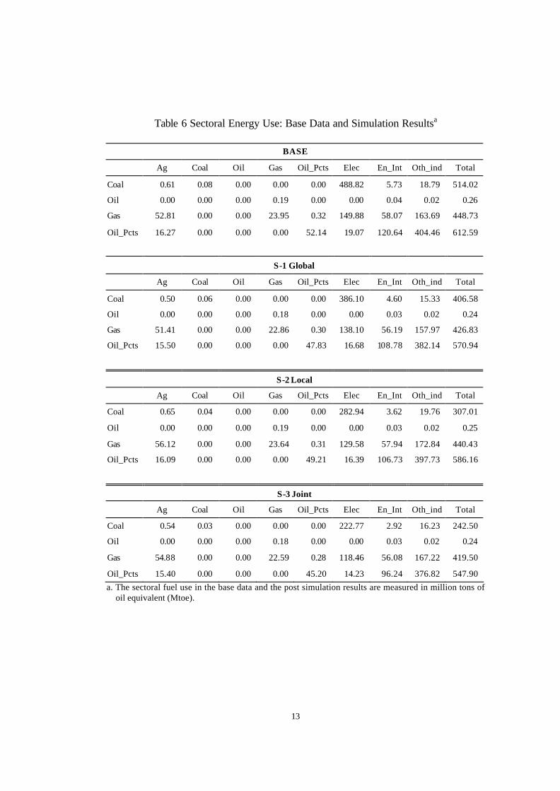
For all of the three scenarios, reductions in firms’ fuels use make great contributions to the overall reductions in fuels use. To get better understanding of the whole story, we further decompose the total changes in firms’ fuel use into sectoral levels. The sectoral fuel use in the base data and the changes in sectoral fuel use for the three scenarios are reported in Table 6. Again, all of the numbers are measured in million tons of oil equivalent (million toe). According to the base data, around 95% of firms’ coal use (488.82 million toe) is utilized in electricity generation. Two-thirds of the natural gas is used in the two sectors: electricity and other industries and services, and each of them accounts for one-third of the total. The majority of oil products is used in the sector of other industries and services (404.46 million toe, 66% of the total).
The post-simulation results show that imposing energy taxes has substantial impacts on sectoral fuel use. For all of the three scenarios, the electricity generation contributes most to the reductions in firms’ use of coal and natural gas. The estimated reductions of coal use by electricity generation are 102.72 million toe for S-1, 205.88 million toe for S-2, and 266.05 million toe for S-3, respectively. In terms of percentage change, the reduced volume of coal use by electricity generation explains above 95% of the total reductions for all of the three scenarios.
The estimated reductions of natural gas use by electricity generation are 11.78 million toe for S-1, 20.30 million toe for S-2, and 31.42 million toe for S-3, respectively. Note that the sector for other industries and services increases its use of natural gas through inter- fuel switching as the tax rates of other types of fuels are relatively high. However, the increases in the total volume of natural gas are modest. For all of the three scenarios, the energy intensive industries and other industries and services account for most of the reductions in the use of oil products. The estimated reductions of oil products by the sectors of energy intensive industries / other industries and services are 11.86 / 22.32 million toe for S-1, 13.91 / 6.73 million toe for S-2, and 24.40 / 27.64 million toe for S-3, respectively.
13
Table 6 Sectoral Energy Use: Base Data and Simulation Resultsa
BASE
Ag Coal Oil Gas Oil_Pcts Elec En_Int Oth_ind Total
Gas 54.88 0.00 0.00 22.59 0.28 118.46 56.08 167.22 419.50
Oil_Pcts 15.40 0.00 0.00 0.00 45.20 14.23 96.24 376.82 547.90 a. The sectoral fuel use in the base data and the post simulation results are measured in million tons of
oil equivalent (Mtoe).
14
Fossil Fuel Intensity
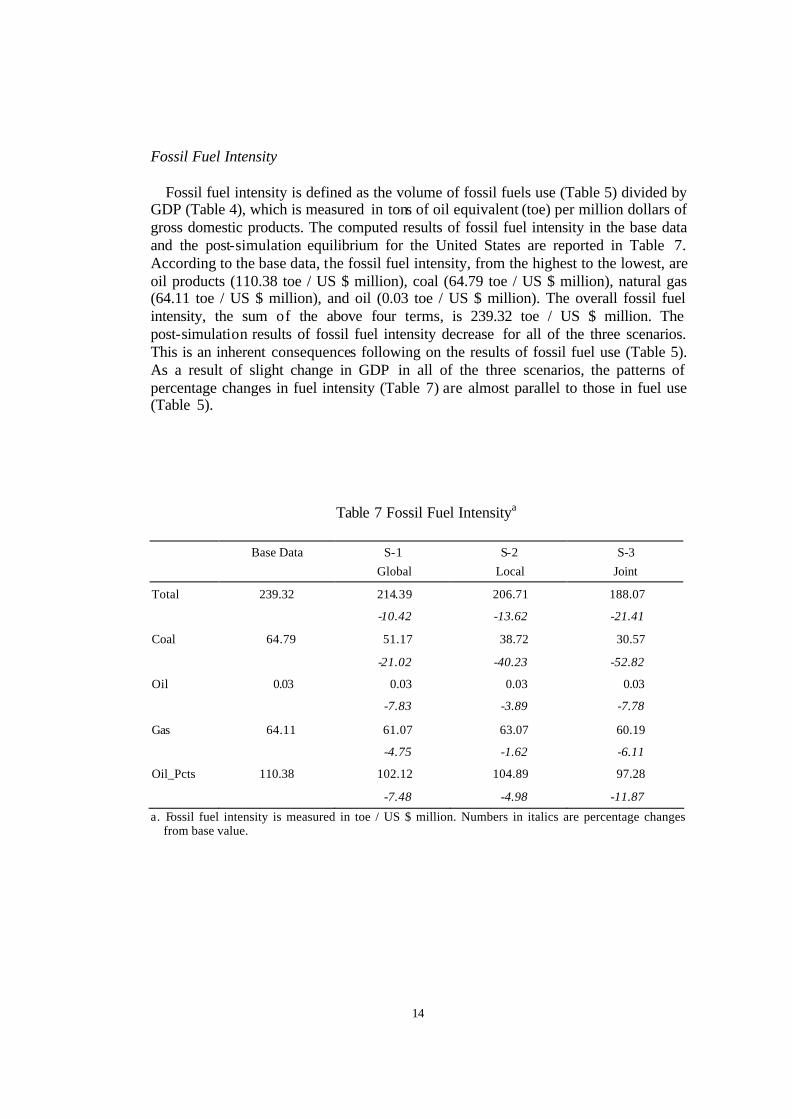
Fossil fuel intensity is defined as the volume of fossil fuels use (Table 5) divided by GDP (Table 4), which is measured in tons of oil equivalent (toe) per million dollars of gross domestic products. The computed results of fossil fuel intensity in the base data and the post-simulation equilibrium for the United States are reported in Table 7. According to the base data, the fossil fuel intensity, from the highest to the lowest, are oil products (110.38 toe / US $ million), coal (64.79 toe / US $ million), natural gas (64.11 toe / US $ million), and oil (0.03 toe / US $ million). The overall fossil fuel intensity, the sum of the above four terms, is 239.32 toe / US $ million. The post-simulation results of fossil fuel intensity decrease for all of the three scenarios. This is an inherent consequences following on the results of fossil fuel use (Table 5). As a result of slight change in GDP in all of the three scenarios, the patterns of percentage changes in fuel intensity (Table 7) are almost parallel to those in fuel use (Table 5).
Table 7 Fossil Fuel Intensitya
Base Data
S-1
Global S-2
Local S-3
Joint
Total 239.32 214.39 206.71 188.07
-10.42 -13.62 -21.41
Coal 64.79 51.17 38.72 30.57
-21.02 -40.23 -52.82
Oil 0.03 0.03 0.03 0.03
-7.83 -3.89 -7.78
Gas 64.11 61.07 63.07 60.19
-4.75 -1.62 -6.11
Oil_Pcts 110.38 102.12 104.89 97.28
-7.48 -4.98 -11.87
a. Fossil fuel intensity is measured in toe / US $ million. Numbers in italics are percentage changes from base value.
15
Environmental Consequences
The carbon emissions and PM10 emissions in the base data and the post-simulation equilibrium for the United States are reported in Table 8. In the base year, carbon emissions and PM10 emissions in the United Sates are 1,499.78 million tons of carbon and 1,522.67 million lbs, respectively. The impact on emissions follows the impacts on fossil fuel energy use. Taxing only global externalities (S-1) also helps to reduce the local externalities at the same time, and vice versa. The emission reductions achieve the maximum in the scenario where the fuels are priced based on their social costs (S-3). The estimated reductions of carbon emissions and PM10 emissions are 378.24 million tons of carbon (25.22%) and 643.48 million lbs (42.26%).
Table 8 Pollution Emissions: Base Data and Simulation Resultsa
-17.02 -31.53 -42.26 a. Carbon emissions and PM10 are measured in million tons of carbon and million lbs, respectively.
Numbers in italics are percentage changes from base value. Reductions in Adverse Health Effects
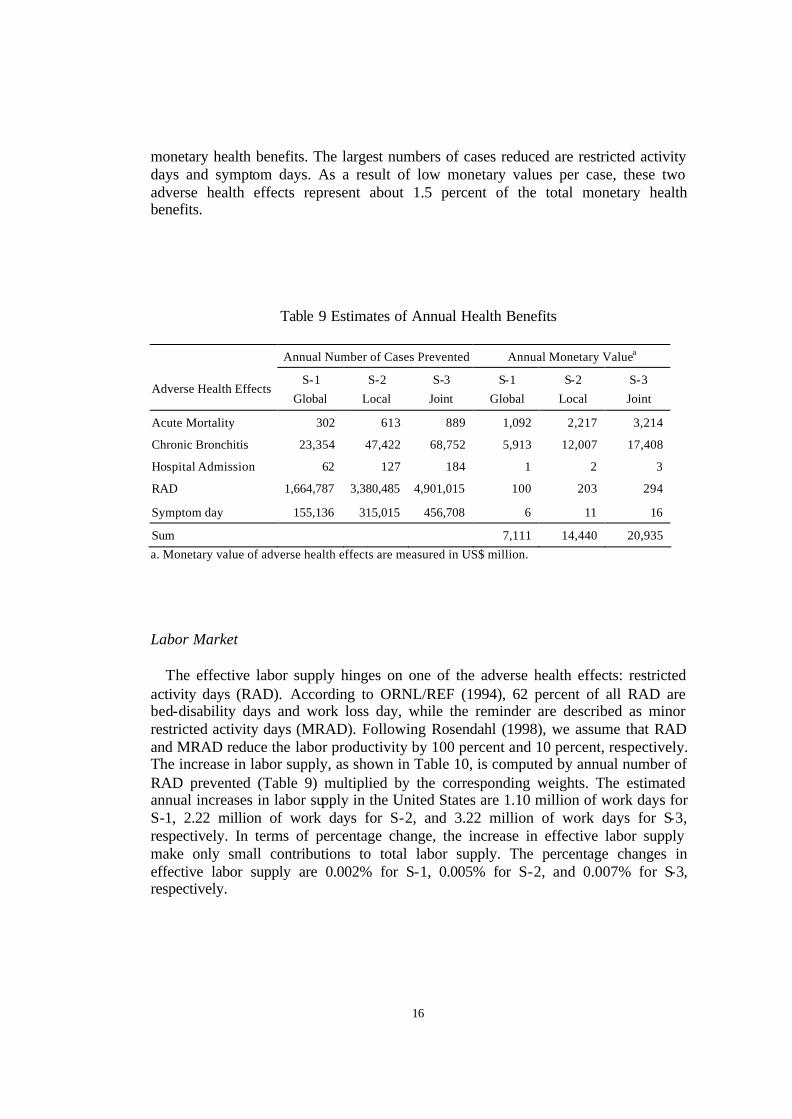
As noted above, the changes in regional adverse health effects are the products of the changes in mean annual ambient concentration levels of air pollution, the concentration-response coefficients and regional population size. Reductions in pollution emissions prevent the occurrence of the illness. The results of the estimated annual health benefits and their monetary values are reported in Table 9. The estimated annual monetary health benefits in the United States are $7,111 million for S-1, $14,440 million for S-2, and $20,935 million for S-3, respectively. For all three scenarios, the monetary health benefit estimates are dominated by the acute mortality and the chronic bronchitis effects. The numbers of cases prevented of these two adverse health effects are relatively small as compared with the restricted activity days and the symptom days, but the high monetary values per case of these two adverse health effects result in large monetary benefits. The combination of the acute mortality reductions and the chronic bronchitis reductions represent about 98 percent of the total
16
monetary health benefits. The largest numbers of cases reduced are restricted activity days and symptom days. As a result of low monetary values per case, these two adverse health effects represent about 1.5 percent of the total monetary health benefits.
Table 9 Estimates of Annual Health Benefits
Annual Number of Cases Prevented Annual Monetary Valuea
Sum 7,111 14,440 20,935 a. Monetary value of adverse health effects are measured in US$ million.
Labor Market
The effective labor supply hinges on one of the adverse health effects: restricted activity days (RAD). According to ORNL/REF (1994), 62 percent of all RAD are bed-disability days and work loss day, while the reminder are described as minor restricted activity days (MRAD). Following Rosendahl (1998), we assume that RAD and MRAD reduce the labor productivity by 100 percent and 10 percent, respectively. The increase in labor supply, as shown in Table 10, is computed by annual number of RAD prevented (Table 9) multiplied by the corresponding weights. The estimated annual increases in labor supply in the United States are 1.10 million of work days for S-1, 2.22 million of work days for S-2, and 3.22 million of work days for S-3, respectively. In terms of percentage change, the increase in effective labor supply make only small contributions to total labor supply. The percentage changes in effective labor supply are 0.002% for S-1, 0.005% for S-2, and 0.007% for S-3, respectively.
17
Table 10 Impacts on Effective Labor Supply
S-1
Global S-2
Local S-3
Joint
Increase in Labor Supplya 1.100 2.220 3.220
0.002 0.005 0.007 a. The increase in labor supply is measured in million of work days. The total labor supply in the base
data is 44,854.14 million of work days. Numbers in italics are percentage changes from base value. Implications for Policy Recommendations
This paper develops a computable general equilibrium (CGE) model to explore the proper design of environmental policies where the use of fossil fuels generates multiple externalities. The externalities are referred to as external costs arising from pollution emissions that threaten the environment and human health, and they are classified into two categories, including climate change and air pollution. The policy in this paper is defined as levying taxes (as a percent of fuel price) on fossil fuels. The main aim of the energy taxes is to reduce the energy consumption and to reduce pollution emissions simultaneously.
The manner we model the interactions between economic activities, fuel use, and environmental consequences is distinct form the existing studies in two ways. First, to reflect the fact that energy use in different sectors has different emission factors, detailed data of sectoral energy use and three-dimensional emission factors (pollutants by fuel type by private consumption or production processes) are incorporated into our empirical model. The incorporation of this feature provides not only more precise estimations of pollution emissions, but also the impacts of energy taxes on the fuel use at sectoral levels. Second, the value-added of this study is the addition of a wide range of different effects such as direct welfare effects, adverse health effects, and productivity effects within an empirical framework intended for analysis of fuel use and its externalities. With a comprehensive description of multiple externalities of fuel use, our empirical model explicitly brings together the jointly produced global and local externalities, and the interactions between the global and local environmental policies.
Three scena rios on energy taxes, including internalization of global externalities alone, internalization of local externalities alone, and joint implementation of the above two policies, are analyzed. The tax rates are set equal to each fuel’s estimated external costs of global and/or local environmental externalities, and they vary substantially by fuel type and by sector because of differences in sectoral emission factors and fuel prices. The design of the simulation scenarios can be interpreted as implementing energy taxes at three different levels, and the focus of this study is to explore how well the taxes correspond to actual environmental costs and the impacts of the taxes on the economy and environment. Internalizing the multiple externalities
18
generated by a single input through combined taxes is equivalent to adding up all of the external costs, and, therefore, the tax rates in the scenario with joint environmental taxes on greenhouse gases and local air pollutants are highest. Consequently, the simulation results from the three scenarios are of quasi- linearity.
According to the original theoretical principles of environmental taxation of A.C. Pigou (1920), the welfare of society will be increased if external environmental costs of energy use are internalized as fuel taxes are paid by the fuel users. Correctly pricing fuels through joint environmental taxes on greenhouse gases and local air pollutants to ensure that all environmental externalities of fossil fuel combustion are accounted for in market mechanisms is theoretically first-best regulatory means. Our numerical results are consistent with this optimal policy rule of “full social costs pricing of energy”: the United States can achieve a higher welfare gain along with lower fuel use and pollution emissions in the third scenario, as compared with the first two scenarios where only global or only local externalities are internalized. The estimated overall welfare gains are $12,308 million, where welfare gains of reductions in climate change damages and in adverse health effects make substantial contributions. Adopting joint environmental taxes leads the highest tax rates on fuel use in the third scenario, which procures substantial reductions in fossil fuels use, and emissions of carbon and air pollutants (PM10), and improvement in fossil fuels intensity. The estimated reductions in the total use of fossil fuels are 405.74 million toe (21.34%). The emissions of carbon and PM10 reduce by 25.22% (378.24 million tons of carbon) and 42.26% (643.48 million lbs), respectively. With respect to the welfare gains from the reductions in adverse health effects, the monetary health benefits estimates are dominated by the acute mortality and the chronic bronchitis effects. The combination of the acute mortality reductions and the chronic bronchitis reductions represent about 98 percent of the total monetary health benefits.
In practice, however, there is a regulatory gap between economists who know theoretical virtues of Pigouvian taxes and political decision-makers who are aware of practical difficulties in the legislation. Public resistance of the new taxes arises from concerns about the possible negative impacts of Pigouvian taxes, such as losses of efficiency or competitiveness. Given the enormous uncertainties surrounding the effects of future climate change, internalizing local air pollution alone is more acceptable since the welfare gains from reductions in adverse health effects and increases in labor productivity are more apparent. Moreover, reducing local air pollution also accompanies ancillary benefits of reductions in carbon emissions and future climate change damages. It should be noted that the benefits from reductions in adverse health effects and increases in labor productivity is of highly geographical sensitivity, and the distribution of the welfare gains within the United States is beyond the scope of this study but is worthy of future research.
19
Appendix
Direct Damage of Global Warming
The impact of greenhouse gases on the global environment depends on their accumulations in the atmosphere (Fankhauser, 1994). The costs of climate change result from changes of vegetation zones on agriculture and silviculture, changes in the occurrence of crop pests and disease-carrying insects, as well as the effects of increased frequencies of extreme events such as heat waves, dry spells and floods. While the scientists and economists have tried to estimate the environmental damage costs from greenhouse gas emissions, there are still problems related to quantification of climate change damage costs.9 Instead of putting our focus on these problems, we just adopt the existing numerical results from the literature on environmental damage costs of greenhouse gas emissions.
Several studies have assessed global costs of climate change in the event of a doubling of pre-industrial greenhouse gas concentration. These studies predict a net damage of 1.5% to 2.5% of current world GNP, or, US$ 270 billion (Frankhauser, cited in Pearce et al., 1994) to US$ 316 billion in the year in which doubling of CO2 is achieved. These point estimates, however, tell us little about the social damage costs of a ton of carbon emitted today. Instead of applying a point estimate of damage in a particular year, we use the present value of expected future climate change damage to represent the direct damage costs. Available estimates of marginal costs of present CO2 emissions range from US$5 to US$ 45 per ton of carbon.10 We adopt the central estimate US$ 20 per ton of carbon provided by Fankhauser (1994) in our model. Coefficients Related to Estimation of Adverse Health Effects
A review of the existing epidemiological literature shows that the main hazardous air pollutants that have significant health impacts include small particulates, especially those measuring less than 10 microns in aerodynamic diameter (PM10) (e.g. Markandya and Pavan, 1999; Alberini et al., 1997; Alberini and Krupnick, 1997; Chestnut et al., 1997; Cropper et al., 1997; Eskeland, 1997; Pope et al., 1995). The term “particulates” includes a number of chemical compounds such as sulfates. However, size is what is considered most important in a normal pollution situation.
9 The main problems related to the quantification of climate change damage costs may be summarized into three categories. First, climate change impacts are extremely complex, with a very large number of different physical endpoints affected. The understanding of the related mechanisms of action in many cases is still poor, and the probability of extreme events is still difficult to assess. Second, following the theoretical foundations of monetization, climate change impacts are valued at national or regional prices. This may be objectionable for ethical reasons, as a life lost in developing countries counts less than a life lost in developed countries. Finally, climate change is a long term problem, so that from an economist’s perspective discounting is an important issue. Different discounting rates may result in different values of environmental damages of greenhouse gas emissions. 10 There is approximately one ton of carbon in every 3.7 tons of CO2.
20
PM10 are particulates small enough to be inhaled into the airways of lungs, and they are sometimes called thoracic particulate matter. PM10 further comprises coarse particulates and fine particulates; the latter with an aerodynamic diameter below 2.5 microns (PM2.5). Both coarse and fine particulates can accumulate in the respiratory system and are associated with numerous adverse health effects. Exposure to coarse particulates is primarily associated with the aggravation of respiratory conditions such as asthma. Fine particulates are most closely associated with adverse health effects including increased hospital admissions, increased respiratory symptoms and disease, and premature death.
The adverse health effects in this paper are defined as the yearly accumulated effects arising from the changes in mean annual ambient concentration levels.11 Estimating these adverse health effects requires four groups of data –emission factors for PM10, baseline mean annual ambient concentration levels for PM10, concentration-response coefficients, and regional population data. By the assumption of linear emissions scaling, the changes in yearly average concentration level for PM10 due to changes in fuel use is the product of the baseline mean annual ambient concentration level and the ratio of post-simulation minus baseline emissions to the total baseline emissions . The post-simulation and baseline emissions are calculated by summing the products of emission factors and sectoral or private energy volume data in the post-simulation and the baseline equilibrium, respectively. The total baseline emissions are the computed baseline emissions divided by the percentage of emissions from fuel combustion.12 The resulting changes in mean annual ambient concentration levels, together with the concentration-response coefficients and regional population size, determine the changes in regional adverse health effects. Now we turn to a detailed discussion of computation processes and the data.
The major assumption under which we estimate the region-wide changes in mean annual ambient concentration levels of PM10 is linear emissions scaling. This technique assumes a linear relationship between changes in emissions and changes in ambient concentration of the emitted pollutant. In other words, the changes in yearly average concentration level for PM10 due to changes in fuel use is defined as the product of the baseline mean annual ambient concentration level and the ratio of post-simulation minus baseline emissions to the total baseline emissions. Mathematically, the changes in yearly average concentration level of pollution i ( i =PM10) can be expressed as (A.1).
11 In other words, we assume that a change in the air concentration variables in a certain period has an effect on health in the same period. 12 Based on EPA publication (National Air Quality and Emissions Trends Report), PM10 emissions from fuel combustion account for 2.7535% of the total emissions.
21
(A.1) BiB
i
Bi
Pi
i CPEEE
C ⋅−
=∆/
where
iC∆ is the changes in yearly average concentration level of pollution i BiC is the baseline concentration level of pollution i PiE is the post-simulation emissions of pollution i from fuel combustion BiE is the baseline emissions of pollution i from fuel combustion
P is the percentage of the emissions from fuel combustion PE B
i / is the total baseline emissions of pollution i
Since the pollutant emissions are primarily dependent on the fuel type and the industrial or private activity processes, the three-dimensional emission factors (pollutants by fuel type by consumption or production) are introduced to capture the proportional relationships between pollution emissions and per unit fuel use. The post-simulation and baseline emissions from fuel combustion are calculated by summing the products of emission factors and sectoral or private energy volume data in the post-simulat ion and the baseline equilibrium, respectively. Mathematically, they can be expressed as (A.2). (A.2) P
jkj k
ijkPi QE ⋅= ∑∑α
Bjk
j kijk
Bi QE ⋅= ∑∑α
where
ijkα is the (three-dimensional) emission factors: pollutant i emitted from per unit fuel j used in consumption or production process k
PjkQ is the volume of fuel j used in consumption or production process k in the
post-simulation equilibrium BjkQ is the volume of fuel j used in consumption or production process k in the
baseline equilibrium The emission factors for industrial production and those for private consumption
are obtained from different sources. With respect to industrial production processes, the three-dimensional emission factors are obtained from several publications of U.S. Environmental Protection Agency, including Compilation of Air Pollutant Emission Factors, AP-42, National Air Pollutant Emission Trends – Procedures Document, and Cost and Quality of Fuels for Electric Utility Plants. The private consumption externalities we focus on in this paper relate to priva te transportation activities. The
22
emission factors are obtained from publication of U.S. Environmental Protection Agency –Section 4.6 (On-Road Vehicle) in Procedures Document for National Emission Inventory, Criteria Air Pollutants 1985-1999. Since the emission factors are in unit of grams per mile, we use transportation statistics from publications of U.S. Department of Transportation – National Transportation Statistics 2001 to convert the primary unit of emission factors to the unit of lbs per toe of gasoline use.
Estimations of adverse health effects caused by the changes in mean annual ambient concentration levels in this paper rely on available epidemiological studies.13 These studies provide “concentration-response” functions that characterize the statistical relationship between changes in health endpoints (response) associated with unit change in ambient levels (concentration) of pollutants in a given time period. The “concentration-response” functions can be expressed in the following form. (A.3) )( ilil CFH ∆=∆ where
lH∆ is the change in frequency or risk of a specific adverse health effect l
iC∆ is the change in concentration of a certain atmospheric pollutant i
liF denotes the estimated quantitative relation between lH∆ and iC∆
Following the results of many epidemiological studies which found that liF is linear or approximately linear functions , we assume liF is a linear function throughout this paper. Equation (A.3) can be hence rewritten as (A.4).
(A.4) ilil CH ∆⋅=∆ π where
liπ are the concentration-response coefficients. The adverse health effect l in our model can be broadly grouped into two
categories – mortality and morbidity effects. The mortality effect includes acute mortality. The morbidity effects include adult chronic bronchitis, hospital admissions for respiratory infections, restricted activity day (RAD), and symptom day. One should note that there are significant differences between the coefficients for mortality effects and those for morbidity effects: the coefficients for mortality effects are measured based on the primary regional death rate whereas the coefficients for morbidity effects are measured in the unit of cases per 100,000 persons. Therefore,
13 As noted in Chestnut(1995), the primary advantage of doing this is that it makes a quantitative assessment feasible with limited research resources and that it uses a great deal of health effects evidence that is readily available.
23
these concentration-response coefficients should be interpreted and applied carefully. For example, “acute mortality caused by an increase in PM10 concentration” should be interpreted as “a n increase of 3/1 mgµ in PM10 concentration is associated with an increase of about 0.104 percent of acute mortality”. The lower and upper limits for the coefficient are 0.064 and 0.145, respectively. On the other hand, “hospital admission for respiratory infections caused by an increase in PM10 concentration” means that “a n increase of 3/1 mgµ in PM10 concentration is associated with an increase of about 0.187 case of hospital admission for respiratory infections per 100,000 persons”. The lower and upper limits for the coefficient are 0.124 and 0.251, respectively.
Therefore, the total numbers of changes in adverse health effect l caused by an increase in concentration of pollutant i in region r with total population rPOP can be expressed as (A.5) and (A.6), respectively.
(A.5) )1000/( rrri
rli
rl POPDRCTH ⋅⋅∆⋅=∆ π for l= mortal health effects
(A.6) )100000/( rri
rli
rl POPCTH ⋅∆⋅=∆ π for l = morbid health effects
where rlTH∆ = changes in adverse health effect l in region r
rDR = death rate (deaths/1000 population) in region r The regional death rate data are obtained from the publication of U.S. Central
Intelligence Agency – The World Factbook 2002. The population data in 1997 are obtained from International Programs Center of US Census Bureau. The population data are disaggregated into three types (Childhood: age 0-14, Adults: age 15-64, and Elder: age 65 and above). Monetary Valuations of the Adverse Health Effects
Adverse health effects result in a number of economic and social consequences, and, therefore, they constitute both financial and non-financial significance to human welfare. The common term used for valuation estimates of premature mortality risks is “value of a statistical life” (VSL), which does not reflect the value of an identifiable life, but instead the value of reducing fatal risks in a population. The financial costs of morbidity, known as cost of illness (COI), 14 include the direct losses to society, stemming from the cost of treatment of each effect (medical cost paid by individuals or insurance companies) plus work loss (lost personal income and lost labor
14 With available market and expenditure data, COI measures have the practical advantages of being easily understood and often readily available. However, they do not reflect the total welfare impact of an adverse health effect, and, therefore, they result in a clear downward bias in the valuation of adverse health effects.
24
productivity). Non- financial costs of morbidity take account of the disutility from pain and discomfort suffered by the individual, altruistic impacts, etc.
A comprehensive monetary valuation for changes in adverse health effects should reflect all costs to the affected individual and to society. This monetary valuation is the maximum willingness to pay (WTP) to reduce the risk of the adverse health effects and all associated costs, or, equivalently, the dollar amount that would cause the affected individual to be indifferent to experiencing an increase in the risk of the adverse health effect. The values of the adverse health effects we use for the United States are the averages of the low, central, and high estimates weighted by the corresponding sele cted probability. Adverse Health Effects and Effective Labor Supply
The total labor force in the base data is measured in numbers of work days, which is the value of the total adult (i.e., a subset of the total population) multiplied by 250.15 The adverse health effect which has an impact on effective labor supply is restricted activity day (RAD), one of the morbidity effects. The acute mortality effect on economic productivity is not considered in our model.16 According to ORNL/REF (1994), 62 percent of all RAD are bed-disability days and work loss day, while the reminder are described as minor restricted activity days (MRAD). Following Rosendahl (1998), we assume that RAD and MRAD reduce the labor productivity by 100 percent and 10 percent, respectively.
15 In other words, we assume that each adult can offer 250 work days per year. 16 Persons who die due to a short-term increase in pollution levels are mainly elderly and chronic ill , and, therefore, they are outside the workforce. It is hence reasonable to believe that the effects of acute mortality have negligible impact on economic activity through a reduced work force.
25
Bibliography Alberini, A., M. Cropper, T.T. Fu, A. Krupnick, J.T. Liu, D. Shaw, and W. Harrington
(1997) “Valuing Health Effects of Air Pollution in Developing Countries: The Case of Taiwan,” Journal of Environmental Economics and Management 34:107-126.
Alberini, A., and A. Krupnick (1997) “Air Pollution and Acute Respiratory Illness:
Evidence from Taiwan and Los Angeles,” American Journal of Agricultural Economics 79(5):1620-1624.
Burniaux, J-M., and T. P. Troung (2002) “GTAP-E: An Energy-Environmental
Version of the GTAP Model,” GTAP Technical Paper No.16, Center for Global Trade Analysis, Purdue University.
Chestnut, L.G., B.D. Ostro, and N. Vichit-Vadakan (1997) “Transferability of Air
Pollution Control Health Benefits Estimates from the United States to Developing Countries: Evidence from the Bangkok Study,” American Journal of Agricultural Economics 79(5):1630-1635.
Cifuentes, L., V.H. Borja-Aburto, N. Gouveia, G. Thurston, and D.L. Davis (2001)
“Hidden Health Benefits of Greenhouse Gas Mitigation,” Science 293(5533): 1257-1259.
Crawford, I., and S. Smith (1995) “Fiscal Instruments for Air Pollution Abatement in
Road Transport,” Journal of Transport Economics and Policy 29(1): 33-51. Cropper, M.L., N.B. Simon, A. Alberini, S. Arora, and P. K. Sharma (1997) “The
Health Benefits of Air Pollution Control in Delhi,” American Journal of Agricultural Economics 79(5):1625-1629.
Dockery, D.W., and C.A. Pope (1994) “Acute Respiratory Effects of Particulates Air
Pollution,” Annual Review of Public Health 15:107-132. EC (European Commission) (1995) ExternE: Externalities of Energy, DG XII,
Volume 1-6. Ekins, P. (1996) “How Large a Carbon Tax is Justified by the Secondary Benefits of
CO2 Abatement?” Resource and Energy Economics 18(2): 161-187. Eskeland, G.S. (1997) “Air Pollution Requires Multipollutant Analysis: The Case of
Santiago, Chile,” American Journal of Agricultural Economics 79(5):1636-1641.
26
Fankhauser, S. (1994) “Evaluating the Social Costs of Greenhouse Gas Emission,” Working Paper GEC 94-1, CSERGE, London.
Halkos, G.E. (1993) “Sulphur Abatement Policy: Implications of Cost Differentials,”
Energy Policy 21(10): 1035-1043. Hertel, T.W., and M.E. Tsigas (1997) “Structure of GTAP,” Chapter 2 in Global
Trade Analysis: Modeling and Applications. T.W. Hertel, ed. New York: Cambridge University Press.
IPCC (1992) Climate Change 1992 - The Supplementary Report to the IPCC
Scientific Assessment. Cambridge: Cambridge University Press. Krewitt, Wolfram (2002) “External Costs of Energy - Do the Answers Match the
Questions? Looking Back at 10 Years of ExternE,” Energy Policy 30:839-848. Lee, T.C. (2004) Essays on Trade and Environmental Policies for an Open Economy.
Ph.D. Dissertation, Department of Applied Economics and Management, Cornell University.
Markandya, A., and M. Pavan (1999) Green Accounting in Europe – Four Case
Studies. Dordrecht: Kluwer Academic Publishers. Miranda, M.L., and B.W. Hale (2002) “A Taxing Environment: Evaluating the
Multiple Objectives of Environmental Taxes,” Environmental Science & Technology 36(24):5289-5295.
Navrud, S. (2001) “Valuing Health Impacts from Air Pollution in Europe: New
Empirical Evidence on Morbidity,” Environmental and Resource Economics 20:305-329.
Norland, D.L. and Y.N. Kim (1998) Price It Right: Energy Pricing and Fundamental
Tax Reform. Washington DC: Alliance to Save Energy. ORNL/REF (Oak Ridge National Laboratory and Resources for the Future) (1994)
External Costs and Benefits of Fuel Cycles, A Study by the U.S. Department of Energy and the Commission of the European Communities, Oak Ridge, TN.
Parry, I.W.H., and R.C. Williams (1999) “A Second-Best Evaluation of Eight Policy
Instruments to Reduce Carbon Emissions,” Resource and Energy Economics 21:347-373.
Pearce, D.W., W.R. Cline, A.N. Achanta, S. Fankhauser, R.K. Pachauri, R.S.J. Tol, P.
Vellinga (1994) Chapter 6: The Social Costs of Climate Change: Greenhouse Damage and the Benefits of Control. IPCC Working Group III.
27
Pope, C.A. III, M.J. Thun, M.M. Namboodri, D.W. Dockery, J.S. Evans, F.E. Speizer, and C.W. Heath (1995) “Particulate Air Pollution as a Predictor of Mortality in a Prospective Study of US Adults,” American Journal of Respiratory Critical Care Medicine 151:669-674.
Rosendahl, K.E. (1998) “Health Effects of Air Pollution and Impacts on Economic
Activity,” Chapter 5 in Social Costs of Air Pollution and Fossil Fuel Use – A Macroeconomic Approach. K.E. Rosendahl, ed. Statistics Norway.
Tsigas, M.E., D. Gray, T.W. Hertel, and B. Krissoff (2001) “Environmental
Consequences of Trade Liberalization in the Western Hemisphere,” in The Sustainability of Long-Term Growth: Socioeconomic and Ecological Perspective. Munasinghe, Mohan, Osvaldo Sunkel and Carlos de Miguel eds. Cheltenham: Edward Elgar.
U.S. Environmental Protection Agency (1999) The Benefits and Costs of the Clean
Air Act 1990 to 2010 - EPA Report to Congress. Electronic access: <http://yosemite.epa.gov/ee/epa/eerm.nsf/efd9186ce4269b8d85256b4300527ad2/490de3d62654580c8525683a007ace54?OpenDocument>.
Vehmas, J., J. Kaivo-oja, J. Luukkanen, and P. Malaska (1999) “Environmental Taxes
on Fuels and Electricity - Some Experiences from the Nordic Countries,” Energy Policy 27:343-355.
Wang, X., and K.R. Smith (1999) “Secondary Benefits of Greenhouse Gas Control:
Health Impacts in China,” Environmental Science and Technology 33(18): 3056-3061.