Page 1
OPTIMAL EXERCISE OF COLLAR TYPEAND MULTIPLE TYPE PERPETUAL
AMERICAN STOCK OPTIONS INDISCRETE TIME WITH LINEAR
PROGRAMMING
a thesis
submitted to the department of industrial engineering
and the graduate school of engineering and science
of bilkent university
in partial fulfillment of the requirements
for the degree of
master of science
By
Emre Kara
June, 2014
Page 2
I certify that I have read this thesis and that in my opinion it is fully adequate,
in scope and in quality, as a thesis for the degree of Master of Science.
Prof. Dr. Mustafa C. Pınar (Advisor)
I certify that I have read this thesis and that in my opinion it is fully adequate,
in scope and in quality, as a thesis for the degree of Master of Science.
Assoc. Prof. Dr. Alper Sen
I certify that I have read this thesis and that in my opinion it is fully adequate,
in scope and in quality, as a thesis for the degree of Master of Science.
Assoc. Prof. Dr. Azer Kerimov
Approved for the Graduate School of Engineering and Science:
Prof. Dr. Levent OnuralDirector of the Graduate School
ii
Page 3
ABSTRACT
OPTIMAL EXERCISE OF COLLAR TYPE ANDMULTIPLE TYPE PERPETUAL AMERICAN STOCK
OPTIONS IN DISCRETE TIME WITH LINEARPROGRAMMING
Emre Kara
M.S. in Industrial Engineering
Supervisor: Prof. Dr. Mustafa C. Pınar
June, 2014
An American option is an option that entitles the holder to buy or sell an
asset at a pre-determined price at any time within the period of the option con-
tract. A perpetual American option does not have an expiration date. In this
study, we solve the optimal stopping problem of a perpetual American stock
option from optimization point of view using linear programming duality under
the assumption that underlying’s price follows a discrete time and discrete state
Markov process. We formulate the problem with an infinite dimensional linear
program and obtain an optimal stopping strategy showing the set of stock-prices
for which the option should be exercised. We show that the optimal strategy
is to exercise the option when the stock price hits a special critical value. We
consider the problem under the following stock price movement scenario: We use
a Markov chain model with absorption at zero, where at each step the stock price
moves up by ∆x with probability p, and moves down by ∆x with probability q
and does not change with probability 1 − (p + q). We examine two special type
of exotic options. In the first case, we propose a closed form formula when the
option is collar type. In the second case we study multiple type options, that are
written on multiple assets, and explore the exercise region for different multiple
type options.
Keywords: Perpetual American options, Collar type options, Multiple type op-
tions, Triple random walk, Difference equations.
iii
Page 4
OZET
YAKA TIPI VE COKLU VARLIKLI VADESIZAMERIKAN HISSE SENEDI OPSIYONLARININ
KESIKLI ZAMANDA DOGRUSAL PROGRAMLAMAILE EN IYI KULLANIM DEGERLERININ
BELIRLENMESI
Emre Kara
Endustri Muhendisligi, Yuksek Lisans
Tez Yoneticisi: Prof. Dr. Mustafa C. Pınar
Haziran, 2014
Amerikan opsiyonu, sahibine bir varlıgı herhangi bir zamanda onceden belir-
lenmis bir fiyata alma ya da satma hakkını verir. Vadesiz Amerikan opsiyonunun
bitis zamanı yoktur. Bu calısmada, opsiyonun yazıldıgı hisse senedinin kesikli
zamanda kesikli degerler aldıgı Markov sureclerini izledigi varsayımıyla dogrusal
programlama yontemleri kullanılarak vadesiz Amerikan opsiyonunun en iyi karı
verecek sekilde ne zaman kullanılması gerektigi problemi ele alınmıstır. Prob-
lem, sonsuz degiskenli dogrusal programlama ile modellenmis ve en iyi opsiyon
kullanım stratejisini veren hisse senedi degerleri belirlenmistir. En iyi kullanım
stratejisinin aslında hisse senedinin belli bir degere ulasır ulasmaz opsiyonun kul-
lanılması oldugu gosterilmistir. Problem, hisse senedinin su sekilde bir hareket
izledigi varsayımıyla modellenmistir: Hisse senedi, 0 degeri aldıgında artık islem
goremeyecegi varsayımını yapan Markov zinciri modelini izler, hisse senedinin
degeri her bir adımda ya p olasılıkla ∆x kadar artar, ya q olasılıkla ∆x kadar
azalır, ya da 1 − (p + q) olasılıkla sabit kalır. Iki farklı egzotik opsiyon tipi in-
celenmistir. Birincisinde, yaka tipi opsiyonlar icin kapalı cozum formulu elde
edilmistir. Ikincisinde ise birden fazla hisse senedi uzerine yazılmıs birkac tip
coklu varlıklı opsiyon icin opsiyonu kullanma alanları belirlenmistir.
Anahtar sozcukler : Vadesiz Amerikan opsiyonları, Yaka tipi opsiyonlar, Coklu
varlıklı opsiyonlar, Uclu rassal yuruyus, Fark denklemleri.
iv
Page 5
Acknowledgement
Foremost, I would like to express my sincere gratitude to my advisor Prof.
Dr. Mustafa C. Pınar for the continuous support of my study and research,
for his patience, motivation, enthusiasm, and immense knowledge. His guidance
helped me in all the time of research and writing of this thesis. I could not have
imagined having a better advisor and mentor for my M.S. study.
Besides my advisor, I would like to thank the rest of my thesis committee:
Assoc. Prof. Dr. Alper Sen, Assoc. Prof. Dr. Azer Kerimov, and Dr. Yosum
Kurtulmaz for their encouragement and insightful comments.
My sincere thanks also goes to my house mate Mustafa Emre Gunduz for his
continuous support throughout the writing period of the thesis, Emre Haliloglu
who has stood as a best friend in my side during my whole master study period
and my friends Ahmet Taha Koru and Ali Ilker Isık for their technical help on
developing numerical analysis of the proposed models.
Last but not the least, I would like to thank my family: my parents Ibrahim
Kara and Aysel Zeynep Kara, my aunt Meral Ayfer Sarp, my uncle Ahmet
Feridun Sarp, and my grandfather Cevat Setkaya, for supporting me during this
thesis period and spiritually throughout my life.
v
Page 6
Contents
1 Introduction 1
1.1 Basic Terminology on Options . . . . . . . . . . . . . . . . . . . . 2
1.2 Motivation . . . . . . . . . . . . . . . . . . . . . . . . . . . . . . . 4
2 Literature Review 6
3 Background 8
3.1 Markov Processes . . . . . . . . . . . . . . . . . . . . . . . . . . . 8
3.2 Potentials and Excessive Functions . . . . . . . . . . . . . . . . . 9
3.3 Optimal Stopping on Markov Processes . . . . . . . . . . . . . . . 10
3.4 The Fundamental Theorem . . . . . . . . . . . . . . . . . . . . . 11
3.5 Triple Random Walk . . . . . . . . . . . . . . . . . . . . . . . . . 11
3.6 Collar Type Options . . . . . . . . . . . . . . . . . . . . . . . . . 12
3.7 Multiple Type Options . . . . . . . . . . . . . . . . . . . . . . . . 13
4 Optimal Stopping for Collar Type Options 14
vi
Page 7
CONTENTS vii
4.1 Primal Problem . . . . . . . . . . . . . . . . . . . . . . . . . . . . 14
4.2 Dual Problem . . . . . . . . . . . . . . . . . . . . . . . . . . . . . 15
4.3 Complementary Slackness Conditions . . . . . . . . . . . . . . . . 15
4.4 Solution Procedure for Primal and Dual Problem . . . . . . . . . 16
4.5 Check the Inequalities . . . . . . . . . . . . . . . . . . . . . . . . 19
4.5.1 Inequalities 4.2 . . . . . . . . . . . . . . . . . . . . . . . . 20
4.5.2 Inequalities 4.1 . . . . . . . . . . . . . . . . . . . . . . . . 20
4.5.3 Inequalities 4.4 . . . . . . . . . . . . . . . . . . . . . . . . 20
4.5.4 Inequalities 4.3 . . . . . . . . . . . . . . . . . . . . . . . . 22
4.5.5 Inequality 4.4 with j = j∗ . . . . . . . . . . . . . . . . . . 23
4.6 Numerical Results . . . . . . . . . . . . . . . . . . . . . . . . . . . 23
4.7 Sensitivity Analysis . . . . . . . . . . . . . . . . . . . . . . . . . . 26
4.7.1 Sensitivity on p and q . . . . . . . . . . . . . . . . . . . . 26
4.7.2 Sensitivity on α . . . . . . . . . . . . . . . . . . . . . . . . 27
4.7.3 Sensitivity on S1 . . . . . . . . . . . . . . . . . . . . . . . 30
4.7.4 Sensitivity on S2 . . . . . . . . . . . . . . . . . . . . . . . 32
5 Optimal Stopping for Multiple Type Options 34
5.1 Primal Problem . . . . . . . . . . . . . . . . . . . . . . . . . . . . 35
5.2 Dual Problem . . . . . . . . . . . . . . . . . . . . . . . . . . . . . 36
5.3 Complementary Slackness Conditions . . . . . . . . . . . . . . . . 36
Page 8
CONTENTS viii
5.4 Exercise Regions . . . . . . . . . . . . . . . . . . . . . . . . . . . 37
5.4.1 Maximum Call Options . . . . . . . . . . . . . . . . . . . . 39
5.4.2 Minimum Call Options . . . . . . . . . . . . . . . . . . . . 40
5.4.3 Average Call Options . . . . . . . . . . . . . . . . . . . . . 41
5.4.4 Spread Options . . . . . . . . . . . . . . . . . . . . . . . . 42
6 Conclusion 43
A GAMS code for the model of collar type options 47
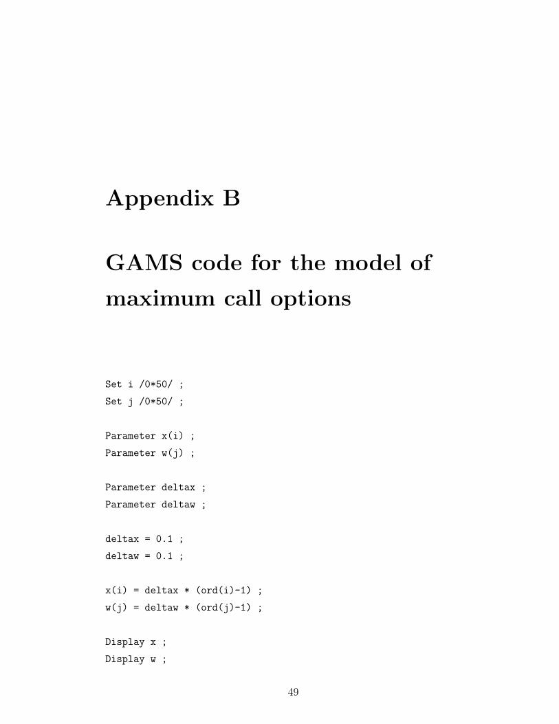
B GAMS code for the model of maximum call options 49
Page 9
List of Figures
4.1 Value and pay-off function (p = 0.35, q = 0.35, α = 0.998, S1 =
0.5, S2 = 1.5, ∆x = 0.1). . . . . . . . . . . . . . . . . . . . . . . . 24
4.2 Calculation of j∗ with proposed closed form formula. . . . . . . . 25
4.3 Value and pay-off function (p = 0.3, q = 0.4, α = 0.998, S1 = 0.5,
S2 = 1.5, ∆x = 0.1). . . . . . . . . . . . . . . . . . . . . . . . . . 26
4.4 Value and pay-off function (p = 0.36, q = 0.34, α = 0.998, S1 =
0.5, S2 = 1.5, ∆x = 0.1). . . . . . . . . . . . . . . . . . . . . . . . 27
4.5 Value and pay-off function (p = 0.35, q = 0.35, α = 0.99, S1 = 0.5,
S2 = 1.5, ∆x = 0.1). . . . . . . . . . . . . . . . . . . . . . . . . . 28
4.6 Value and pay-off function (p = 0.35, q = 0.35, α = 0.999, S1 =
0.5, S2 = 1.5, ∆x = 0.1). . . . . . . . . . . . . . . . . . . . . . . . 29
4.7 Value and pay-off function (p = 0.35, q = 0.35, α = 0.998, S1 =
0.3, S2 = 1.5, ∆x = 0.1). . . . . . . . . . . . . . . . . . . . . . . . 30
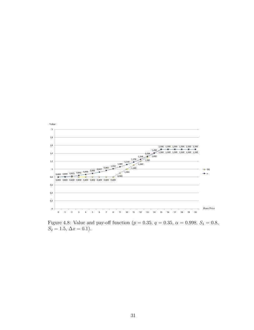
4.8 Value and pay-off function (p = 0.35, q = 0.35, α = 0.998, S1 =
0.8, S2 = 1.5, ∆x = 0.1). . . . . . . . . . . . . . . . . . . . . . . . 31
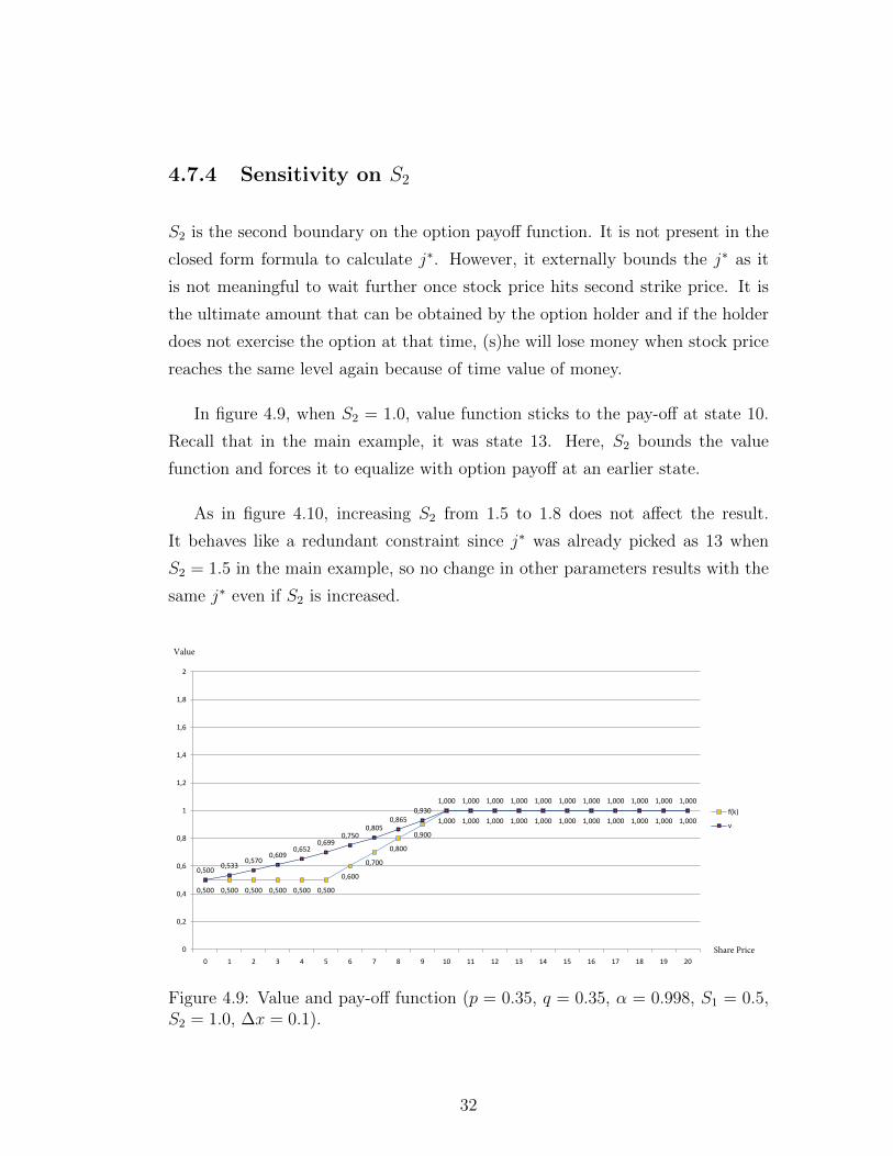
4.9 Value and pay-off function (p = 0.35, q = 0.35, α = 0.998, S1 =
0.5, S2 = 1.0, ∆x = 0.1). . . . . . . . . . . . . . . . . . . . . . . . 32
ix
Page 10
LIST OF FIGURES x
4.10 Value and pay-off function (p = 0.35, q = 0.35, α = 0.998, S1 =
0.5, S2 = 1.8, ∆x = 0.1). . . . . . . . . . . . . . . . . . . . . . . . 33
5.1 Exercise Region for Maximum Call Options (p = 0.35, q = 0.35,
α = 0.998, S = 2, ∆x = 0.1). . . . . . . . . . . . . . . . . . . . . . 39
5.2 Exercise Region for Minimum Call Options (p = 0.35, q = 0.35,
α = 0.998, S = 2, ∆x = 0.1). . . . . . . . . . . . . . . . . . . . . . 40
5.3 Exercise Region for Average Call Options (p = 0.35, q = 0.35,
α = 0.998, S = 2, ∆x = 0.1). . . . . . . . . . . . . . . . . . . . . . 41
5.4 Exercise Region for Spread Call Options (p = 0.35, q = 0.35,
α = 0.998, S = 2, ∆x = 0.1). . . . . . . . . . . . . . . . . . . . . . 42
Page 11
Chapter 1
Introduction
Mathematical finance is one of the fields of applied mathematics, mainly con-
cerned with financial markets. This field derives and extends mathematical mod-
els by assuming market prices given while financial economics might investigate
the structural reasons behind it. There are two main research branches in math-
ematical finance: One is derivative pricing which we will be dealing with in this
thesis, and the other one is risk and portfolio management.
A derivative can be defined as financial instrument whose value depends on
(or derives from) the values of other, more basic, underlying variables [1]. For
example, a stock option is a derivative whose value is dependent on the price
of the underlying stock. The most common underlying assets are commodities,
stocks, bonds, interest rates and currencies. In this thesis, we will focus on stocks
as an underlying asset.
In the last 30 years, derivatives have become increasingly important in finance.
They can be used for either risk management by hedging, meaning that providing
offsetting compensation in case of an undesired event, or speculation which means
a financial bet to make money.
Derivatives are traded on financial markets like stocks, currencies, and com-
modities, as well. Most traded derivatives are futures and options. A future
1
Page 12
contract is an agreement between two parties to buy or sell an asset at a certain
time in the future for a certain price. An option contract, on the other hand,
is an agreement between two parties to have the right but not the obligation to
buy or sell an asset at a certain time in the future for a certain price. The main
difference between these two derivatives is that for futures, there is an obligation
to honor the contract at the expiration date, but not for options. That is why
there is no cost to enter a future contract but there is for options, called premium.
Determining the premium is the fundamental question for both buyer and
seller of an option contract in the financial market. It is called the fair price of
an option. Valuation of options have some complexities compared to valuation
of traditional equities. It is even more complicated when the option holder has
right to use the contract at any time within the contract period which is the case
in so-called American type options. In this study, we will construct an optimal
trading strategy for an American option holder under the assumption that stock
price follows discrete time discrete state triple random walk process. Optimal
trading strategy will show to the holder at which states (s)he will use the option
contract to get the best expected future pay-off.
1.1 Basic Terminology on Options
A call option gives the owner the right, but not the obligation, to buy an asset
at a specified price within a specified time. A put option gives the owner the
right, but not the obligation, to sell an asset in a similar fashion. Strike price of
an option is the fixed price at which the owner of the option can buy or sell the
underlying asset. The date on which the option expires is called maturity date.
When the option holder uses the contract, meaning that (s)he buys or sells the
underlying asset at strike price, we say that the holder has exercised the option.
In a given state of the world, the amount that the option holder gains or loses as
a function of underlying’s payoff is called option payoff. In this work, we will use
S for strike price, T for maturity date, the real-valued function f : E → R for
the option payoff where E is the set of all possible states of the world.
2
Page 13
A European option can be exercised only at the expiration date, i.e., single
pre-defined point in time. On the other hand, an American option can be exer-
cised at any time before the expiration date. If there is no expiration date, it is
called perpetual option. In this thesis, we work on perpetual American options.
American type options require dynamic valuation process since the option holder
must observe the underlying’s price through time and decide on a time to exercise
to maximize his/her earnings. This type of analysis is not required in European
type options since exercise date is fixed during the agreement.
American and European types of options are called plain vanilla options and
these types of options are used in financial markets most frequently. Options
which do not fall this category is called exotic options. Exotic options are rarely
used compared to plain vanilla options but they are more complex derivatives
and constitute an interesting background in the derivative pricing literature.
Assume that for some state of the world x ∈ E, the payoff of the underlying is
represented by X(x). For the call option holder, if X(x) is greater than the strike
price S at the maturity date, it is meaningful for the holder to exercise the option
for an immediate gain of X(x)− S, since the contract gives her the right to buy
a unit of the underlying at the price S. Then, by selling this unit in the original
market for its real market value X(x), the owner can have the specified gain. If
the price of the underlying, however, is lower than S, it will not be profitable
to exercise the option because the same asset is already available cheaper in the
exchange market. For a call option, the payoff function corresponds to:
f(x) = maxX(x)− S, 0 = (X(x)− S)+
In the case of a put option, the condition on trade is reversed, and the owner has
the right to sell the option at the maturity date. Note that this strategy is only
profitable when X(x) < S, hence, the payoff of a put option is:
f(x) = maxS −X(x), 0 = (S −X(x))+
Note that, in this study, an option is assumed to be call option unless otherwise
stated.
3
Page 14
1.2 Motivation
Let us consider a perpetual American option holder. Since there is no maturity
date for the contract, the holder will decide when to exercise the option only based
on the observations on the underlying stock price movement. The objective of the
trader is to find the states where (s)he should exercise the option to obtain the
best expected payoff. The purpose of this study is based on this important need
of the option holder. In this study, we will characterize the optimal exercising
strategy so that the option holder will know at which states to exercise the option
and at which states to wait further in order to obtain more with respect to the
expected pay-off.
Suppose that underlying stock follows a stochastic process Xt on the state
space E. For any initial state x and any time t, expected payoff at time t can
be denoted as E[f(Xt)|X0 = x]. Let us introduce a discount factor α (a num-
ber slightly less than one) to account for the fact that future dollars are worth
less than present dollars. Value function v for any option is represented by the
maximum of all such functions over any future time t, that is
v(x) = maxt∈T
Ex[αtf(Xt)
].
This value function v tells both to the seller and buyer of the contract that fair
price of the option is v(x) if the current stock price is x. In each period, the
option holder observes current stock price x, and decides either to exercise the
option or keep it for one more period. This decision is made by looking at the
gap between value function v and option payoff f . Note that it is not possible to
have v(x) < f(x) since the time-index set involves time zero. Another important
note is that delaying the decision to exercise when v cannot beat f(x) will clearly
be suboptimal, due to the time value of money.
Exercise region can be characterized by a subset OPT of state space E such
that for all x ∈ OPT , v(x) = f(x). For all x /∈ OPT , v(x) must be greater than
f(x), meaning that expected payoff of future gains is greater than current option
payoff, therefore, option holder should wait further to gain more. This region is
called continuation region.
4
Page 15
Optimal trading strategy is to exercise the option immediately once we have
v(x) = f(x), and to keep option as long as v(x) > f(x). In this thesis, our
aim is to find the correct value function and set OPT to tell the trader optimal
exercising strategy.
In this work, we assume that (1) stock price follows a discrete time discrete
state triple random walk, (2) discount factor α ∈ (0, 1) is used for the time value
of money, and (3) option is perpetual American option with no expiration date.
Basically, we will deal with two different special cases of this problem. First,
we will solve the problem when the option is collar type. Second, we will explore
the exercise region when option is multiple stock options which is written on more
than one stock (two different stocks in our case). These two types of options are
exotic options and details will be given in corresponding chapters.
5
Page 16
Chapter 2
Literature Review
Financial market instruments can be divided into two distinct species. There
are the underlying stocks, shares, bonds, currencies; and their derivatives, claims
that promise some payment or delivery in the future contingent on an underlying’s
behavior. Pricing of this second type, derivative pricing is well established and
documented research area in mathematical finance. Since options are widely used
derivatives in the financial market, they have taken researcher’s attention more
than other derivative instruments. This field of research has again two distinctive
branches, based on being European or American type option. We are focusing
on optimal strategy of American type perpetual stock options written on stocks
which follows discrete time discrete state triple random walks.
Option pricing has well-known history and there are many books and papers
written on this field of study. Comprehensive treatments of option pricing can
be found in Hobson’s survey [2], if reader is interested in specifically of American
options, (s)he can refer to Myneni’s [3] surveys. Hull’s text [1] is a good reference
for fundamental models in derivative pricing such as Black-Scholes option pricing
model.
Option pricing literature started by Bachelier [4], he studied European type
options. Later, Samuelson [5] provided a comprehensive treatment on the theory
of option pricing. With the contribution of Black and Scholes [6] and Merton
6
Page 17
[7], option pricing literature has become a well-established research field. In their
work, Black and Scholes show that in a frictionless and arbitrage-free market, the
price of an option solves a special differential equation, a variant of the heat equa-
tion arising in physical problems. Their assumption that the stock price follows
a geometric Brownian motion has been a very key and much cited assumption.
The problem of determining correct prices for American type contingent
claims was first handled by McKean upon a question posed by Samuelson (see
appendix of [8]). In his response, McKean transformed the problem of pricing
American options into a free boundary problem. The formal treatment of the
problem from an optimal stopping perspective was later done by Moerbeke [9]
and Karatzas [10], who used hedging arguments for financial justification. Wong,
in a recent study, has collected the optimal stopping problems arising in the
financial markets [11].
In this thesis, we want to provide a different approach to solve American
option pricing problem in the perspective of linear programming when stock price
follows discrete time discrete state triple random walk. Our aim is to characterize
the exercise region to show the option holder when to exercise the option. It is
well known that the value function of an optimal stopping problem for a Markov
process is the minimal excessive function majorizing the pay-off of the reward
process (see [12] and [13]). With this property of the value function, the problem
can be structured as an infinite dimensional linear model and solved by linear
programming duality concepts. This approach is first used in [14] to treat singular
stochastic control problems. Then, Vanderbei and Pınar [15] use this approach to
propose an alternative method for the pricing of American perpetual warrants.
In their work, they solve the problem when stock price follows simple random
walk and underlying option is plain vanilla option. In this thesis, we will solve
the problem when stock price follows triple random walk, meaning that stock
price can remain at the same price with some probability, and underlying option
is collar type option which is one of the favorite exotic options used for hedging.
Next, we will model the problem when option is multiple type, i.e., option is
written on more than one stock, and explore the exercise region.
7
Page 18
Chapter 3
Background
This chapter contains mathematical definitions and main concepts that will be
used in the remaining part of the thesis. This develops a base to approach this
problem from the linear programming perspective and details can be found in
[13].
3.1 Markov Processes
Let the triplet (Ω,F , P ) be a probability space.
Definition 3.1.1. A stochastic process X = Xt, t ∈ T with the state space E
is a collection of E-valued random variables indexed by a set T , often interpreted
as the time. X is a discrete-time stochastic process if T is countable and a
continuous-time stochastic process if T is uncountable. Likewise, X is called a
discrete-state stochastic process if E is countable and called a continuous-state
stochastic process if E is an uncountable set.
We model the stock price movement as a triple random walk which is a classical
example of stochastic processes. We use memoryless property for stock price
movement model, i.e., future of the process only depends on the current state of
the process. This property is called Markov property.
8
Page 19
Definition 3.1.2. A stochastic process X having the property,
PX(t+ h) = y |X(s),∀s ≤ t = PX(t+ h) = y |X(t)
for all h > 0 is said to have the Markov property. A stochastic process with the
Markov property is called a Markov process.
In our study, stock price follows discrete time discrete state Markov process
and by the Markov property, next state of stock price is only dependent to current
state.
3.2 Potentials and Excessive Functions
Potentials and excessive functions are the fundamental concepts in optimal stop-
ping literature. They allow us to link stochastic processes and outcomes. Here
are some important definitions from Chapter 7 of [13].
Definition 3.2.1. A real-valued function g : E → R is called the reward function
of a stochastic process X.
Definition 3.2.2. Let g : E → R be a reward function defined on E. The
function Rg : E × T → R defined as
Rgt(i) = Ei∞∑h=0
g(Xt+h)
is called the potential of g.
Definition 3.2.3. Let g : E → R be a reward function defined on E and α ∈(0, 1]. The function Rαg : E × T → R defined as
Rαgt(i) = Ei∞∑h=0
αng(Xt+h)
is called the α-potential of g.
9
Page 20
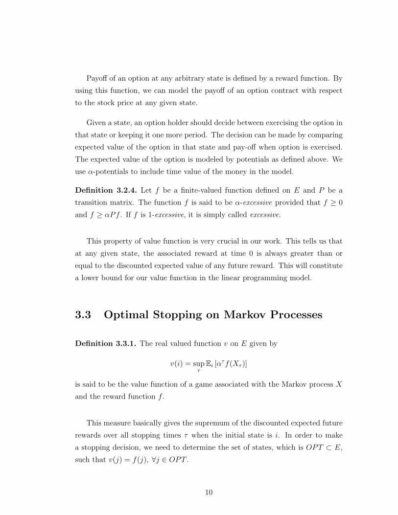
Payoff of an option at any arbitrary state is defined by a reward function. By
using this function, we can model the payoff of an option contract with respect
to the stock price at any given state.
Given a state, an option holder should decide between exercising the option in
that state or keeping it one more period. The decision can be made by comparing
expected value of the option in that state and pay-off when option is exercised.
The expected value of the option is modeled by potentials as defined above. We
use α-potentials to include time value of the money in the model.
Definition 3.2.4. Let f be a finite-valued function defined on E and P be a
transition matrix. The function f is said to be α-excessive provided that f ≥ 0
and f ≥ αPf . If f is 1-excessive, it is simply called excessive.
This property of value function is very crucial in our work. This tells us that
at any given state, the associated reward at time 0 is always greater than or
equal to the discounted expected value of any future reward. This will constitute
a lower bound for our value function in the linear programming model.
3.3 Optimal Stopping on Markov Processes
Definition 3.3.1. The real valued function v on E given by
v(i) = supτ
Ei [ατf(Xτ )]
is said to be the value function of a game associated with the Markov process X
and the reward function f .
This measure basically gives the supremum of the discounted expected future
rewards over all stopping times τ when the initial state is i. In order to make
a stopping decision, we need to determine the set of states, which is OPT ⊂ E,
such that v(j) = f(j), ∀j ∈ OPT .
10
Page 21
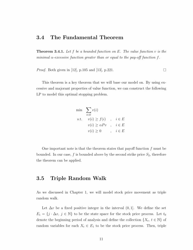
3.4 The Fundamental Theorem
Theorem 3.4.1. Let f be a bounded function on E. The value function v is the
minimal α-excessive function greater than or equal to the pay-off function f .
Proof. Both given in [12], p.105 and [13], p.221.
This theorem is a key theorem that we will base our model on. By using ex-
cessive and majorant properties of value function, we can construct the following
LP to model this optimal stopping problem.
min∑i∈E
v(i)
s.t. v(i) ≥ f(i) , i ∈ Ev(i) ≥ αPv , i ∈ Ev(i) ≥ 0 , i ∈ E
One important note is that the theorem states that payoff function f must be
bounded. In our case, f is bounded above by the second strike price S2, therefore
the theorem can be applied.
3.5 Triple Random Walk
As we discussed in Chapter 1, we will model stock price movement as triple
random walk.
Let ∆x be a fixed positive integer in the interval (0, 1]. We define the set
E1 = j · ∆x, j ∈ N to be the state space for the stock price process. Let t0
denote the beginning period of analysis and define the collection Xt, t ∈ N of
random variables for each Xt ∈ E1 to be the stock price process. Then, triple
11
Page 22
random walk on E1 can be defined by letting:
Xt+1 =
Xt + ∆x w.p. p
Xt −∆x w.p. q
Xt w.p. 1− p− q
for each period t ∈ N and Xt ∈ E1 − 0.
State 0 is an absorbing state; as stock price hits zero, it means associated
company goes bankrupt and stock price will never be able to go back to any
positive value.
3.6 Collar Type Options
Collar type options are used basically for hedging purposes if holder already has
a stock in hand. This type of options allow the holder to gain some amount if
stock prices goes up but it puts a cap on the gain in return for putting a floor on
the downside in order to prevent risk of big stock price decline.
A collar type option is created by an investor being (1) long the underlying
stock, (2) long a put option at strike price S1, and (3) short a call option at strike
price S2.
The payoff of collar type options are as follows [16]:
f(x) = minmaxX(x), S1, S2
When option is exercised, if stock price is lower than first strike price, then holder
will get first strike even if actual stock price is lower. If stock price is between
two strikes, holder will get actual amount of stock. If stock price is greater than
second strike price, then holder will get second strike even if stock has greater
value than second strike. With this strategy, holder guarantees a payoff between
two levels and limits herself for downside risk in return for sacrificing upside gain.
12
Page 23
3.7 Multiple Type Options
In Chapter 6 of [17], Detemple considered American options written on multiple
underlying assets. In his book, he studied different cases such as options written
on minimum, average, and maximum of two assets in continuous time finance
point of view.
Among those three multiple type options, we will consider and model max-call
options. These type of options are exotic options and rarely used in trade market.
However, it is an attractive and challenging research area since value and payoff
function is in third dimension in this case which makes it complicated to find
exercise region.
Given two stocks X and W which follows discrete time discrete state random
walk, payoff function of max-call option written on these two stocks is as follows:
f(x,w) = maxmaxX(x),W (w) − S, 0 = (maxX(x),W (w) − S)+
At any given state, option holder observes stock price level of both stocks and
decides based on the comparison of maximum of both stock prices and strike
price.
13
Page 24
Chapter 4
Optimal Stopping for Collar
Type Options
4.1 Primal Problem
Under the triple random walk assumption, the problem is modeled by the follow-
ing infinite dimensional LP:
minimize∞∑j=0
vj
s.t. vj ≥ fj, j ≥ 0,
vj ≥ α(pvj+1 + qvj−1 + (1− p− q)vj), j ≥ 1.
where xj = j∆x, vj = v(xj), fj = f(xj), and f(xj) = minmaxxj, S1, S2.
This problem stands for the optimal stopping problem of a perpetual collar
type American option written on a stock following triple random walk. If there
exists an optimal solution for this problem, based on the gap between v and f ,
the option holder will find out on which states to exercise the contract, and on
which states to wait further.
Therefore, our aim is to solve this problem optimally, and characterize the
14
Page 25
exercise region.
4.2 Dual Problem
The solution procedure is based on linear programming duality. Therefore, next
step is to find the dual problem to the primal problem above. The associated
dual problem is
maximize∞∑j=0
fjyj
s.t. y0 − αqz1 = 1,
y1 + (1− α(1− p− q))z1 − αqz2 = 1,
yj − αpzj−1 + (1− α(1− p− q))zj − αqzj+1 = 1, j ≥ 2,
yj ≥ 0, j ≥ 0,
zj ≥ 0, j ≥ 1.
Here, yj’s and zj’s are dual variables correspond to first and second set of
constraints of the primal problem, respectively.
4.3 Complementary Slackness Conditions
Based on the primal and dual problem, let us write the complementary slackness
conditions:
(fj − vj)yj = 0, j ≥ 0,
(α(pvj+1 + qvj−1 + (1− p− q)vj)− vj)zj = 0, j ≥ 1,
v0(1− y0 + αqz1) = 0,
v1(1− y1 − (1− α(1− p− q)z1) + αqz2) = 0,
vj(1− yj + αpzj−1 − (1− α(1− p− q)zj) + αqzj+1) = 0, j ≥ 2,
15
Page 26
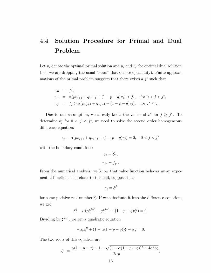
4.4 Solution Procedure for Primal and Dual
Problem
Let vj denote the optimal primal solution and yj and zj the optimal dual solution
(i.e., we are dropping the usual “stars” that denote optimality). Finite approxi-
mations of the primal problem suggests that there exists a j∗ such that
v0 = f0,
vj = α(pvj+1 + qvj−1 + (1− p− q)vj) > fj, for 0 < j < j∗,
vj = fj > α(pvj+1 + qvj−1 + (1− p− q)vj), for j∗ ≤ j.
Due to our assumption, we already know the values of v∗ for j ≥ j∗. To
determine v∗j for 0 < j < j∗, we need to solve the second order homogeneous
difference equation:
vj − α(pvj+1 + qvj−1 + (1− p− q)vj) = 0, 0 < j < j∗
with the boundary conditions:
v0 = S1,
vj∗ = fj∗ .
From the numerical analysis, we know that value function behaves as an expo-
nential function. Therefore, to this end, suppose that
vj = ξj
for some positive real number ξ. If we substitute it into the difference equation,
we get
ξj − α(pξj+1 + qξj−1 + (1− p− q)ξj) = 0.
Dividing by ξj−1, we get a quadratic equation
−αpξ2 + (1− α(1− p− q))ξ − αq = 0.
The two roots of this equation are
ξ− =α(1− p− q)− 1−
√(1− α(1− p− q))2 − 4α2pq
−2αp,
16
Page 27
ξ+ =α(1− p− q)− 1 +
√(1− α(1− p− q))2 − 4α2pq
−2αp.
where we used ξ− to denote the larger root and ξ+ for the smaller root. The
general solution to the difference equation is therefore
vj = c+ξj+ + c−ξ
j−.
From the first boundary condition v0 = S1, we get that c+ + c− = S1. This
relation together with the second boundary condition vj∗ = fj∗ gives
c+ =fj∗ − S1ξ
j∗
−
ξj∗
+ − ξj∗
−
Hence,
vj =
(fj∗ − S1ξ
j∗
−
ξj∗
+ − ξj∗
−
)(ξj+ − ξ
j−) + S1ξ
j−, 0 < j < j∗.
Now, let us solve for zj. Since vj∗ is optimal for primal problem, it has to
satisfy CS conditions. We know that v∗j 6= fj for 0 < j < j∗, thus, y∗j = 0 when
0 < j < j∗ and last CS condition reduces to:
(1− α(1− p− q))zj − α(pzj−1 + qzj+1) = 1, 0 < j < j∗.
with the boundary conditions:
z0 = 0,
zj∗ = 0.
First boundary condition is just an additional variable which does not affect the
problem formulation. Second boundary condition is obtained from the second CS
condition; since for j ≥ j∗, first part of the multiplication is nonzero which forces
zj to be 0.
We need a particular solution to the equation and the general solution to the
associated homogeneous equation. For a particular solution, we try a constant
value
zj ≡ c.
17
Page 28
Substituting into the difference equation, we get c = 1/(1− α).
Let us write the equation for zj in different form:
zj − α(qzj+1 + pzj−1 + (1− p− q)zj) = 1, 0 < j < j∗.
This homogeneous equation is exactly the same as the equation for vj except
with p and q interchanged. Hence the general solution, which is the sum of the
particular and the homogeneous, is given by
zj =1
1− α+ c+ζ
j+ + c−ζ
j−
where
ζ+ = 1/ξ− =α(1− p− q)− 1−
√(1− α(1− p− q))2 − 4α2pq
−2αq,
ζ− = 1/ξ+ =α(1− p− q)− 1 +
√(1− α(1− p− q))2 − 4α2pq
−2αq.
Using the boundary conditions to eliminate the two undetermined constants, we
get
zj =
(1− ζj
∗
− − 1
ζj∗
− − ζj∗
+
ζj+ −ζj∗
+ − 1
ζj∗
+ − ζj∗
−ζj−
)/(1− α), 0 < j < j∗.
It only remains to show the values of yj. The dual constraint ensure that
yj = 1 for j > j∗ since zj = 0 in this region. Then,
yj =
1 + αqz1 j = 0
0 0 < j < j∗
1 + αpzj∗−1 j = j∗
1 j > j∗
18
Page 29
To summarize, we have
vj =
S1 j = 0
(fj∗ − S1ξj∗
− )
(ξj+−ξ
j−
ξj∗
+ −ξj∗−
)+ S1ξ
j−, 0 < j < j∗
fj j∗ ≤ j
zj =
(
1− ζj∗− −1
ζj∗− −ζ
j∗+
ζj+ −ζj∗
+ −1ζj∗
+ −ζj∗−ζj−
)/(1− α) 0 < j < j∗
0 j∗ ≤ j
yj =
1 + αqz1 j = 0
0 0 < j < j∗
1 + αpzj∗−1 j = j∗
1 j∗ < j
Now, we have candidate optimal solutions vj, yj, and zj to the primal and dual
problems. The only thing left we have to show is that these candidate solutions
satisfy all constraints in both primal and dual problems.
4.5 Check the Inequalities
Inequalities we need to check are as follows:
yj ≥ 0, j ≥ 0, (4.1)
zj ≥ 0, j ≥ 1, (4.2)
vj ≥ fj, j ≥ 0, (4.3)
vj ≥ α(pvj+1 + qvj−1 + (1− p− q)vj), j ≥ 1. (4.4)
In [15], a methodology to check these inequalities for a plain vanilla option
under simple random walk assumption is proposed. We will follow the same
methodology with some modifications for collar type options under triple random
walk assumption.
19
Page 30
4.5.1 Inequalities 4.2
For j ≥ j∗, it directly follows from the formula of zj. We are done when we show
that it holds for 0 < j < j∗.
By a contrary, let us assume that zj < 0 for some 0 < j < j∗. Then, there
must be a k at which zk is negative and a local minimum:
zk ≤ zk−1 and zk ≤ zk+1.
If j′ is the index of the local minimum, that is j′ = k, from the last CS condition
and yj = 0 for 0 < j < j∗, we have:
(1− α(1− p− q))zj′ = 1 + α(pzj′−1 + qzj′+1)
≥ 1 + α(pzj′ + qzj′)
zj′ − αzj′ + αpzj′ + αqzj′ ≥ 1 + αpzj′ + αqzj′
zj′(1− α) ≥ 1.
which implies that zj′ ≥ 1/(1 − α). This contradicts with zj′ being negative. If
j′ is not the index of the local minimum then we either have zj′−1 > zj′ > zj′+1
or zj′−1 < zj′ < zj′+1. Note that due to the boundary conditions, that are
z0 = 0, zj∗=0, we must have at least one local minimum as we change j′ towards
0 or j∗ which will again lead to a contradiction. Hence, zj ≥ 0 for all 0 < j < j∗
4.5.2 Inequalities 4.1
We proved that zj ≥ 0 for j ≥ 1. p, q, and α are nonnegative. Combining these
facts, from the formula of yj, it is easy to see that yj ≥ 0 for j ≥ 0.
4.5.3 Inequalities 4.4
These hold trivially for j < j∗. For j ≥ j∗, We will split it by j > j∗ and j = j∗.
Let us start with the former case. To show that inequality holds, we need make
an assumption. We will assume that αp ≤ 1/3 , αq ≤ 1/3, and α(1−p−q) ≤ 1/3.
20
Page 31
Let j = j∗+k, k = 1, 2, . . . and assume αp ≤ 1/3, αq ≤ 1/3, and α(1−p−q) ≤1/3. Then,
αpvj∗+k+1 + αqvj∗+k−1 + α(1− p− q)vj∗+k= αpfj∗+k+1 + αqfj∗+k−1 + α(1− p− q)fj∗+k
≤ 1
3fj∗+k+1 +
1
3fj∗+k−1 +
1
3fj∗+k
=1
3(fj∗ + (k + 1)∆x) +
1
3(fj∗ + (k − 1)∆x) +
1
3(fj∗ + k∆x)
= fj∗ + k∆x
= fj∗+k
= vj∗+k.
The one just given suffices but is not necessary. A necessary and sufficient con-
dition is obtained by recalling that vj = fj for j > j∗. It is easy to see after some
simple algebraic manipulation that for j = j∗ + k, and k = 1, 2, . . . we have
αpvj∗+k+1 + αqvj∗+k−1 + α(1− p− q)vj∗+k ≤ vj∗+k
αpfj∗+k+1 + αqfj∗+k−1 + α(1− p− q)fj∗+k ≤ fj∗+k
Since
fj∗+k = fj∗ + k∆x
We have
fj∗ + k∆x ≥ αpfj∗ + αp(k + 1)∆x+ αqfj∗ + αq(k − 1)∆x+ α(1− p− q)fj∗+α(1− p− q)k∆x
fj∗ + k∆x ≥ αp∆x− αq∆x+ αfj∗ + αk∆x
fj∗(1− α) ≥ α∆x(p− q) + k(α− 1)∆x
Since k(α−1)∆x is negative (α < 1), the left hand side is maximized at k = 1.
Hence, (4.4) holds with vj = fj if and only if
(1− α)fj∗ ≥ α∆x(p− q) + (α− 1)∆x.
We’ll come back to the inequality (4.4) for j = j∗ after we consider inequalities
(4.3).
21
Page 32
4.5.4 Inequalities 4.3
For j ≥ j∗, vj = fj from the formula for vj. We need to show that vj ≥ fj for
j ≤ j∗. In order to have these inequalities hold for j < j∗, we need to pick
j∗ ∈ K :=
k : (fk − S1ξ
k−)
(ξk−1+ − ξk−1−
ξk+ − ξk−
)+ S1ξ
k−1− > fk−1
.
We need to assume that K is nonempty. We need to show that K has finite
number of elements.In order to show it, let us observe the following inequality for
k ∈ K:
(fk − S1ξk−)
(ξk−1+ − ξk−1−
ξk+ − ξk−
)+ S1ξ
k−1− > fk−1
It can be written as:
ξk−1+ − ξk−1−
ξk+ − ξk−1− ξ−>
fk−1 − S1ξk−1−
fk − S1ξk−
The LHS behaves as 1/ξ− and the right hand as 1 for large k, which implies
that k cannot grow without bound since ξ− > 1.
For an hj and the assumption that j∗ ∈ K, we have that vj∗ = hj∗ and
vj∗−1 > hj∗−1. Suppose that vj′ < hj′ for some j′ < j∗. Then the sequence
uj := vj − hj must have a local maximum at some point, say k, strictly between
j′ and j∗. That is, uk > uk−1 and uk > uk+1. But, we also have
uk = vk − hk= α(pvk+1 + qvk−1 + (1− p− q)vk)−
1
3(hk+1 + hk−1 + hk)
≤ 1
3(vk+1 + vk−1 + vk)−
1
3(hk+1 + hk−1 + hk)
=1
3(uk+1 + uk−1 + uk)
< uk.
It is a contradiction. Therefore, uj can’t have a local maximum and therefore vj
cannot dip below hj and this ends the proof.
22
Page 33
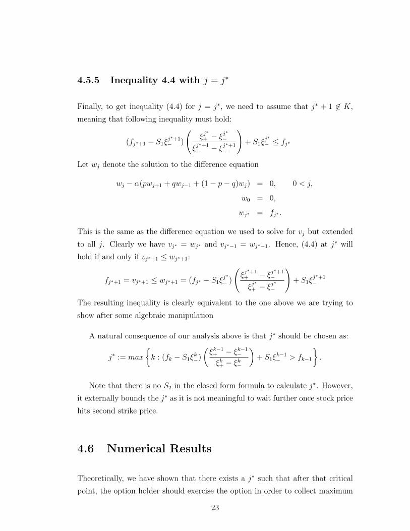
4.5.5 Inequality 4.4 with j = j∗
Finally, to get inequality (4.4) for j = j∗, we need to assume that j∗ + 1 6∈ K,
meaning that following inequality must hold:
(fj∗+1 − S1ξj∗+1− )
(ξj∗
+ − ξj∗
−
ξj∗+1
+ − ξj∗+1−
)+ S1ξ
j∗
− ≤ fj∗
Let wj denote the solution to the difference equation
wj − α(pwj+1 + qwj−1 + (1− p− q)wj) = 0, 0 < j,
w0 = 0,
wj∗ = fj∗ .
This is the same as the difference equation we used to solve for vj but extended
to all j. Clearly we have vj∗ = wj∗ and vj∗−1 = wj∗−1. Hence, (4.4) at j∗ will
hold if and only if vj∗+1 ≤ wj∗+1:
fj∗+1 = vj∗+1 ≤ wj∗+1 = (fj∗ − S1ξj∗
− )
(ξj∗+1
+ − ξj∗+1−
ξj∗
+ − ξj∗
−
)+ S1ξ
j∗+1−
The resulting inequality is clearly equivalent to the one above we are trying to
show after some algebraic manipulation
A natural consequence of our analysis above is that j∗ should be chosen as:
j∗ := max
k : (fk − S1ξ
k−)
(ξk−1+ − ξk−1−
ξk+ − ξk−
)+ S1ξ
k−1− > fk−1
.
Note that there is no S2 in the closed form formula to calculate j∗. However,
it externally bounds the j∗ as it is not meaningful to wait further once stock price
hits second strike price.
4.6 Numerical Results
Theoretically, we have shown that there exists a j∗ such that after that critical
point, the option holder should exercise the option in order to collect maximum
23
Page 34
gain among all other expected payoffs and we give a closed form formulation to
calculate j∗.
If we solve the finite approximation of infinite dimensional LP for 20 states, for
chosen parameters p, q, α, S1, S2 (shown in the definition of figure), the obtained
results are presented in figure 4.1.
0,500 0,500 0,500 0,500 0,500 0,500
0,600
0,700
0,800
0,900
1,000
1,100
1,200
1,300
1,400
1,500 1,500 1,500 1,500 1,500 1,500
0,5000,537
0,5770,620
0,6670,717
0,7720,831
0,895
0,964
1,039
1,119
1,206
1,300
1,400
1,500 1,500 1,500 1,500 1,500 1,500
0
0,2
0,4
0,6
0,8
1
1,2
1,4
1,6
1,8
2
0 1 2 3 4 5 6 7 8 9 10 11 12 13 14 15 16 17 18 19 20
f(k)
v
Share Price
Value
Figure 4.1: Value and pay-off function (p = 0.35, q = 0.35, α = 0.998, S1 = 0.5,S2 = 1.5, ∆x = 0.1).
Optimal v values and payoff function f are graphed. For chosen parameters,
finite approximation of our LP model says that j∗ is obtained at state 13, i.e.,
when stock price hits 1.3 (note that ∆x = 0.1), option should be exercised.
One immediate observation from the figure is that, as claimed, until critical
value, value function stands above the payoff function. It means that keeping
option for one more period is more beneficial than exercising the option. In those
states, vj > fj. After the critical point j ≥ j∗, value function sticks to the payoff
function (vj = fj) and continues to grow together.
For given parameters, proposed formula suggests to pick maximum index j
24
Page 35
k f(k) ξ+(k-1) ξ-(k-1) ξ+(k) ξ-(k) result f(k-1) v
0 0,5 0,500
1 0,5 1,000 1,000 0,927 1,079 0,500 0,5 0,537
2 0,5 0,927 1,079 0,860 1,163 0,499 0,5 0,577
3 0,5 0,860 1,163 0,797 1,255 0,497 0,5 0,620
4 0,5 0,797 1,255 0,739 1,353 0,496 0,5 0,667
5 0,5 0,739 1,353 0,685 1,460 0,494 0,5 0,717
6 0,6 0,685 1,460 0,635 1,574 0,575 0,5 0,772
7 0,7 0,635 1,574 0,589 1,698 0,661 0,6 0,831
8 0,8 0,589 1,698 0,546 1,832 0,749 0,7 0,895
9 0,9 0,546 1,832 0,506 1,976 0,839 0,8 0,964
10 1 0,506 1,976 0,469 2,131 0,930 0,9 1,039
11 1,1 0,469 2,131 0,435 2,298 1,022 1 1,119
12 1,2 0,435 2,298 0,403 2,479 1,114 1,1 1,206
13 1,3 0,403 2,479 0,374 2,674 1,206 1,2 1,300
14 1,4 0,374 2,674 0,347 2,884 1,299 1,3 1,400
15 1,5 0,347 2,884 0,321 3,110 1,392 1,4 1,500
16 1,5 0,321 3,110 0,298 3,355 1,393 1,5 1,500
17 1,5 0,298 3,355 0,276 3,618 1,395 1,5 1,500
18 1,5 0,276 3,618 0,256 3,903 1,396 1,5 1,500
19 1,5 0,256 3,903 0,238 4,210 1,396 1,5 1,500
20 1,5 0,238 4,210 0,220 4,540 1,397 1,5 1,500
Figure 4.2: Calculation of j∗ with proposed closed form formula.
as j∗ which makes the LHS of the expression greater than fk−1. In this example,
state 13 is the last state that makes LHS greater than RHS, therefore 13 is chosen
as j∗. (See figure 4.2)
Thus, results from the solution of LP model and output of closed form formula
coincides. Hence, obtaining exercising strategy using proposed formula provides
computational efficiency.
Note that the given closed form formula works even if the assumption αp ≤ 1/3
is violated. Low interest rates (α very close to one) and up probability greater
than 1/3 are very likely in any stock market. Therefore, it is enough to check
necessary and sufficient condition obtained which is as follows:
25
Page 36
(1− α)fj∗ ≥ α∆x(p− q) + (α− 1)∆x.
4.7 Sensitivity Analysis
In this section, we will investigate how exercising strategy can be affected by the
changes in parameters.
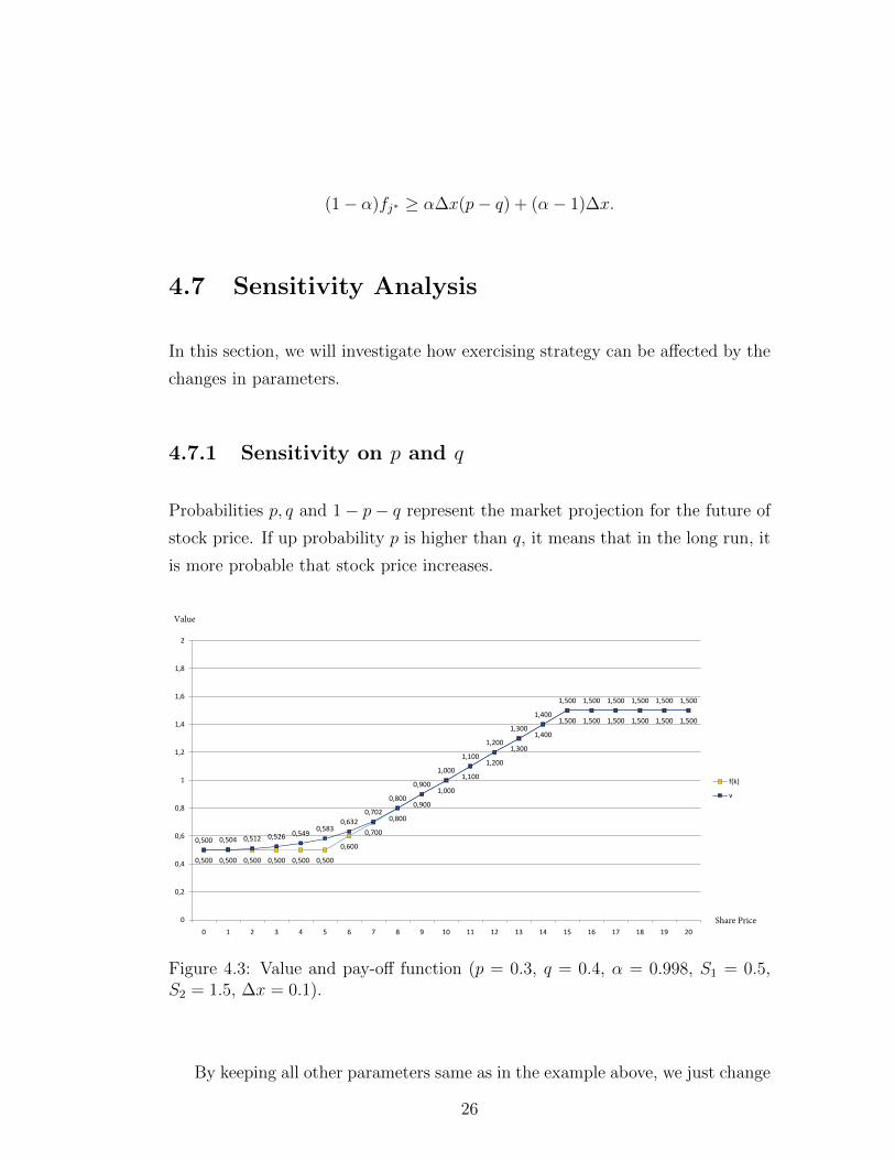
4.7.1 Sensitivity on p and q
Probabilities p, q and 1− p− q represent the market projection for the future of
stock price. If up probability p is higher than q, it means that in the long run, it
is more probable that stock price increases.
0,500 0,500 0,500 0,500 0,500 0,500
0,600
0,700
0,800
0,900
1,000
1,100
1,200
1,300
1,400
1,500 1,500 1,500 1,500 1,500 1,500
0,500 0,504 0,512 0,526 0,5490,583
0,632
0,702
0,800
0,900
1,000
1,100
1,200
1,300
1,400
1,500 1,500 1,500 1,500 1,500 1,500
0
0,2
0,4
0,6
0,8
1
1,2
1,4
1,6
1,8
2
0 1 2 3 4 5 6 7 8 9 10 11 12 13 14 15 16 17 18 19 20
f(k)
v
Share Price
Value
Figure 4.3: Value and pay-off function (p = 0.3, q = 0.4, α = 0.998, S1 = 0.5,S2 = 1.5, ∆x = 0.1).
By keeping all other parameters same as in the example above, we just change
26
Page 37
up and down probabilities to see their impacts on j∗.
If we decrease up probability to 0.3 and increase down probability to 0.4, j∗
is chosen as 8 instead of 13. (See figure 4.3) It means that, since the probability
that stock prices go up is relatively lower, it is more beneficial to exercise the
option at an earlier state.
0,500 0,500 0,500 0,500 0,500 0,500
0,600
0,700
0,800
0,900
1,000
1,100
1,200
1,300
1,400
1,500 1,500 1,500 1,500 1,500 1,500
0,5000,559
0,6170,676
0,7350,795
0,8560,919
0,9831,049
1,117
1,188
1,261
1,338
1,417
1,500 1,500 1,500 1,500 1,500 1,500
0
0,2
0,4
0,6
0,8
1
1,2
1,4
1,6
1,8
2
0 1 2 3 4 5 6 7 8 9 10 11 12 13 14 15 16 17 18 19 20
f(k)
v
Share Price
Value
Figure 4.4: Value and pay-off function (p = 0.36, q = 0.34, α = 0.998, S1 = 0.5,S2 = 1.5, ∆x = 0.1).
In figure 4.4, we graphed the opposite case, i.e., probability that stock price
goes up is relatively higher than the one in main example. As expected, optimal
strategy is to wait more until j∗ = 15 as market is relatively more favorable for
this stock.
4.7.2 Sensitivity on α
The parameter α stands for time value of money in the model. Our model is very
much dependent on the choice of α. For small and high (very close to 1) α values,
j∗ will position at the extremes, at S1, or S2.
27
Page 38
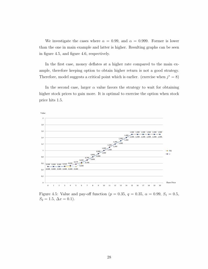
We investigate the cases where α = 0.99, and α = 0.999. Former is lower
than the one in main example and latter is higher. Resulting graphs can be seen
in figure 4.5, and figure 4.6, respectively.
In the first case, money deflates at a higher rate compared to the main ex-
ample, therefore keeping option to obtain higher return is not a good strategy.
Therefore, model suggests a critical point which is earlier. (exercise when j∗ = 8)
In the second case, larger α value favors the strategy to wait for obtaining
higher stock prices to gain more. It is optimal to exercise the option when stock
price hits 1.5.
0,500 0,500 0,500 0,500 0,500 0,500
0,600
0,700
0,800
0,900
1,000
1,100
1,200
1,300
1,400
1,500 1,500 1,500 1,500 1,500 1,500
0,500 0,500 0,500 0,510 0,5340,574
0,630
0,705
0,800
0,900
1,000
1,100
1,200
1,300
1,400
1,500 1,500 1,500 1,500 1,500 1,500
0
0,2
0,4
0,6
0,8
1
1,2
1,4
1,6
1,8
2
0 1 2 3 4 5 6 7 8 9 10 11 12 13 14 15 16 17 18 19 20
f(k)
v
Share Price
Value
Figure 4.5: Value and pay-off function (p = 0.35, q = 0.35, α = 0.99, S1 = 0.5,S2 = 1.5, ∆x = 0.1).
28
Page 39
0,500 0,500 0,500 0,500 0,500 0,500
0,600
0,700
0,800
0,900
1,000
1,100
1,200
1,300
1,400
1,500 1,500 1,500 1,500 1,500 1,500
0,5000,551
0,6030,657
0,7120,770
0,8300,893
0,9571,025
1,096
1,169
1,246
1,327
1,412
1,500 1,500 1,500 1,500 1,500 1,500
0
0,2
0,4
0,6
0,8
1
1,2
1,4
1,6
1,8
2
0 1 2 3 4 5 6 7 8 9 10 11 12 13 14 15 16 17 18 19 20
f(k)
v
Share Price
Value
Figure 4.6: Value and pay-off function (p = 0.35, q = 0.35, α = 0.999, S1 = 0.5,S2 = 1.5, ∆x = 0.1).
29
Page 40
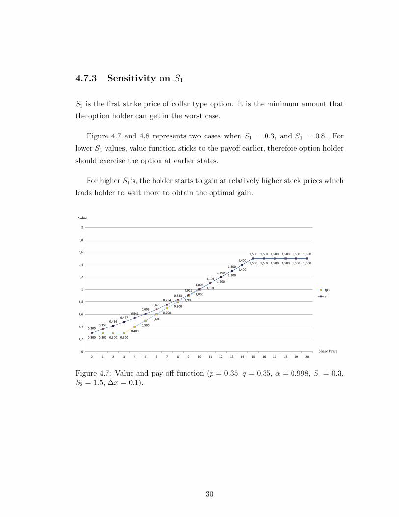
4.7.3 Sensitivity on S1
S1 is the first strike price of collar type option. It is the minimum amount that
the option holder can get in the worst case.
Figure 4.7 and 4.8 represents two cases when S1 = 0.3, and S1 = 0.8. For
lower S1 values, value function sticks to the payoff earlier, therefore option holder
should exercise the option at earlier states.
For higher S1’s, the holder starts to gain at relatively higher stock prices which
leads holder to wait more to obtain the optimal gain.
0,300 0,300 0,300 0,300
0,400
0,500
0,600
0,700
0,800
0,900
1,000
1,100
1,200
1,300
1,400
1,500 1,500 1,500 1,500 1,500 1,500
0,3000,357
0,4160,477
0,5410,609
0,679
0,754
0,833
0,916
1,005
1,100
1,200
1,300
1,400
1,500 1,500 1,500 1,500 1,500 1,500
0
0,2
0,4
0,6
0,8
1
1,2
1,4
1,6
1,8
2
0 1 2 3 4 5 6 7 8 9 10 11 12 13 14 15 16 17 18 19 20
f(k)
v
Share Price
Value
Figure 4.7: Value and pay-off function (p = 0.35, q = 0.35, α = 0.998, S1 = 0.3,S2 = 1.5, ∆x = 0.1).
30
Page 41
0,800 0,800 0,800 0,800 0,800 0,800 0,800 0,800 0,800
0,900
1,000
1,100
1,200
1,300
1,400
1,500 1,500 1,500 1,500 1,500 1,500
0,800 0,809 0,823 0,842 0,8650,893
0,9270,965
1,0101,060
1,1161,178
1,248
1,324
1,408
1,500 1,500 1,500 1,500 1,500 1,500
0
0,2
0,4
0,6
0,8
1
1,2
1,4
1,6
1,8
2
0 1 2 3 4 5 6 7 8 9 10 11 12 13 14 15 16 17 18 19 20
f(k)
v
Share Price
Value
Figure 4.8: Value and pay-off function (p = 0.35, q = 0.35, α = 0.998, S1 = 0.8,S2 = 1.5, ∆x = 0.1).
31
Page 42
4.7.4 Sensitivity on S2
S2 is the second boundary on the option payoff function. It is not present in the
closed form formula to calculate j∗. However, it externally bounds the j∗ as it
is not meaningful to wait further once stock price hits second strike price. It is
the ultimate amount that can be obtained by the option holder and if the holder
does not exercise the option at that time, (s)he will lose money when stock price
reaches the same level again because of time value of money.
In figure 4.9, when S2 = 1.0, value function sticks to the pay-off at state 10.
Recall that in the main example, it was state 13. Here, S2 bounds the value
function and forces it to equalize with option payoff at an earlier state.
As in figure 4.10, increasing S2 from 1.5 to 1.8 does not affect the result.
It behaves like a redundant constraint since j∗ was already picked as 13 when
S2 = 1.5 in the main example, so no change in other parameters results with the
same j∗ even if S2 is increased.
0,500 0,500 0,500 0,500 0,500 0,500
0,600
0,700
0,800
0,900
1,000 1,000 1,000 1,000 1,000 1,000 1,000 1,000 1,000 1,000 1,000
0,5000,533
0,5700,609
0,6520,699
0,7500,805
0,8650,930
1,000 1,000 1,000 1,000 1,000 1,000 1,000 1,000 1,000 1,000 1,000
0
0,2
0,4
0,6
0,8
1
1,2
1,4
1,6
1,8
2
0 1 2 3 4 5 6 7 8 9 10 11 12 13 14 15 16 17 18 19 20
f(k)
v
Share Price
Value
Figure 4.9: Value and pay-off function (p = 0.35, q = 0.35, α = 0.998, S1 = 0.5,S2 = 1.0, ∆x = 0.1).
32
Page 43
0,500 0,500 0,500 0,500 0,500 0,500
0,600
0,700
0,800
0,900
1,000
1,100
1,200
1,300
1,400
1,500
1,600
1,700
1,800 1,800 1,800
0,5000,537
0,5770,620
0,6670,717
0,7720,831
0,895
0,964
1,039
1,119
1,206
1,300
1,400
1,500
1,600
1,700
1,800 1,800 1,800
0
0,2
0,4
0,6
0,8
1
1,2
1,4
1,6
1,8
2
0 1 2 3 4 5 6 7 8 9 10 11 12 13 14 15 16 17 18 19 20
f(k)
v
Share Price
Value
Figure 4.10: Value and pay-off function (p = 0.35, q = 0.35, α = 0.998, S1 = 0.5,S2 = 1.8, ∆x = 0.1).
33
Page 44
Chapter 5
Optimal Stopping for Multiple
Type Options
Multiple type options are options which are written on more than one asset. A
standard example is the case of an index option that is based on the value of a
portfolio of assets. Options on the S&P 100, which have traded on the Chicago
Board of Options Exchange (CBOE) are American options on a value weighted
index of 100 stocks. Options on the maximum of two or more assets can be
found in firms choosing among mutually exclusive investment alternatives, or in
employment switching decisions by agents. Gasoline crack spread options traded
in New York Mercantile Exchange (NYMEX) are examples for multiple type
spread options.
In this thesis, we will study multiple type options written on two assets. We
will consider 4 different types of multiple options. These are maximum, minimum,
average, and spread options. In the main part, we will work on maximum call
options which have payoff structures as in the following:
f(x,w) = maxmaxX(x),W (w) − S, 0 = (maxX(x),W (w) − S)+
There are two underlying stocks, denoted as X, and W , and the option holder
gain the difference between maximum of two stock prices and strike price if the
maximum of those stock prices is greater than strike price; (s)he does not exercise
34
Page 45
the option if it is less than strike, because in that case, there is no gain.
In this chapter, we will model the problem again with an infinite dimensional
LP as in Chapter 4. Note that we need two indices to include both stocks in
our model and it makes the problem complicated to solve by following the same
methodology. Instead of coming up with a closed form formula to calculate critical
optimal stopping point here, we will explore the exercise region for different kinds
of multiple type options.
We assume that both stocks follow different triple random walk process. We
will use px, and pw for up probabilities for stock X, and W , respectively. In a
same manner, we will use qx, and qw for down probabilities. And we will define
rx, and rw for 1− (px + qx), and 1− (pw + qw) to simplify the model.
Based on those assumptions, by the fundamental theorem, we model the pri-
mal problem as follows:
5.1 Primal Problem
The primal problem is
minimize∞∑i=0
∞∑j=0
vi,j
s.t. vi,j ≥ fi,j, i, j ≥ 0,
vi,j ≥ α(pxpwvi+1,j+1 + rxpwvi,j+1 + qxpwvi−1,j+1
+pxrwvi+1,j + rxrwvi,j + qxrwvi−1,j
+pxqwvi+1,j−1 + rxqwvi,j−1 + qxqwvi−1,j−1), i, j ≥ 1.
where xi = i∆x, wj = j∆x, vi,j = v(xi, wj), fi,j = f(xi, wj), and f(xi, wj) =
maxmaxxi, wj − S, 0.
35
Page 46
5.2 Dual Problem
The associated dual problem is
maximize∞∑i=0
∞∑j=0
fi,jyi,j
s.t. y0,0 − αqxqwz1,1 = 1,
y1,1 + (1− αrxrw)z1,1 − αqxqwz2,2 − αrxqwz1,2 − αqxrwz2,1 = 1,
y0,1 − αqxrwz1,1 − αqxqwz1,2 = 1,
y1,0 − αrxqwz1,1 − αqxqwz2,1 = 1,
y0,j − αqxpwz1,j−1 − αqxrwz1,j − αqxqwz1,j+1 = 1, j ≥ 2,
yi,0 − αpxqwzi−1,1 − αrxqwzi,1 − αqxqwzi+1,1 = 1, i ≥ 2,
y1,j + (1− αrxrw)z1,j − αrxqwz1,j+1 − αqxqwz2,j+1 − αqxrwz2,j−αqxpwz2,j−1 − αrxpwz1,j−1 = 1, j ≥ 2,
yi,1 + (1− αrxrw)zi,1 − αqxrwzi+1,1 − αqxqwzi+1,2 − αrxqwzi,2−αpxqwzi−1,2 − αpxrwzi−1,1 = 1, i ≥ 2,
yi,j + (1− αrxrw)zi,j − αqxqwzi+1,j+1 − αrxqwzi,j+1 − αpxqwzi−1,j+1
−αqxrwzi+1,j − αpxrwzi−1,j − αqxpwzi+1,j−1
−αrxpwzi,j−1 − αpxpwzi−1,j−1 = 1, i, j ≥ 2,
yi,j ≥ 0, i, j ≥ 0,
zi,j ≥ 0, i, j ≥ 1.
5.3 Complementary Slackness Conditions
Based on these primal and dual problems, we can write CS conditions. We skip
to write all conditions but the important one:
(vi,j − (α(pxpwvi+1,j+1 + rxpwvi,j+1 + qxpwvi−1,j+1
+ pxrwvi+1,j + rxrwvi,j + qxrwvi−1,j
+ pxqwvi+1,j−1 + rxqwvi,j−1 + qxqwvi−1,j−1))zj = 0, i, j ≥ 0
36
Page 47
Crucial part to solve this problem is to solve the following second order ho-
mogeneous difference equation
vi,j − (α(pxpwvi+1,j+1 + rxpwvi,j+1 + qxpwvi−1,j+1
+ pxrwvi+1,j + rxrwvi,j + qxrwvi−1,j
+ pxqwvi+1,j−1 + rxqwvi,j−1 + qxqwvi−1,j−1) = 0, i, j ≥ 0
with the boundary conditions:
v0,0 = 0,
vi∗,j∗ = fi∗,j∗ .
We could not solve this equation to come up with a similar closed form formula
for vi∗,j∗ , i∗, and j∗. We leave this part as a further research area. Instead, we
will use the primal problem and explore exercise regions for maximum, minimum,
average, and spread type multiple options. It will reveal the optimal exercising
strategy for the option holder by telling at which (i, j) stock price pairs (s)he
should exercise the option.
5.4 Exercise Regions
An increasing number of contractual rewards and obligations, held by economic
entities, involve options that are written on multiple underlying assets. Some of
the payoffs that have become fairly common include options on the maximum
of several asset prices (max-options), options on the minimum of several prices
(min-options), options on an average of prices (portfolio options) and options on
the difference between two prices (spread options)[17]. Contingent claims with
these characteristics can be found on financial exchanges, in over-the-counter
transactions, in cash flows generated by investment decisions of firms and in
executive compensation plans.
For options written on single assets, we have shown that there exists a critical
point after which it is optimal to exercise the option. Intuition suggests that
the same must be true for multiple type options. However, the determination
37
Page 48
of optimal strategy for multiple type options is not as straightforward as in the
single asset case. The presence of multiple prices, that jointly determine the
exercise region, is an obvious complication. Some of the basic insights from the
single asset type options do not carry over when several prices affect the payoff.
Let us give an example for such a situation. The fundamental intuition from
single asset case is that for large stock price values, it is optimal to exercise the
option. However, if we study maximum call options, they have a property called
diagonal property. On the diagonal of the stock price pairs matrix, stock prices
are equal to each other. For the sake of simplicity, let us assume that both stocks
follow the same simple random walk with both up and down probabilities are
equal to 0.5. Then, the probability of an increase in any one of the underlying
asset prices over the next increment of time is roughly equal to 0.5. But the
probability of an increase in the maximum of two prices is about 0.75. The
max-option holder has therefore much better chance of improving his/her payoff
by waiting, than the holder of an option on a single underlying asset. Even if
the stock prices are high, it might not be optimal to exercise the option on the
diagonal for max-call options.
The multivariate nature of these claims ultimately results in complex decision
making. Precise description of the exercise regions become useful for accurate
decision making, as well as for pricing and risk management purposes.
We solve the finite approximation of our infinite dimensional model for some
chosen parameters and explore the exercise and continuation region for four dif-
ferent multiple type options. Note that 1’s in the figures represent the stock price
pairs at which the options should be exercised, meaning that collection of 1’s
in the figures stands for exercise region. Empty regions stand for continuation
region in which option holder should keep the option.
38
Page 49
5.4.1 Maximum Call Options
The payoff function of maximum call options is represented as:
f(xi, wj) = maxmaxxi, wj − S, 0.
0 1 2 3 4 5 6 7 8 9 10 11 12 13 14 15 16 17 18 19 20 21 22 23 24 25 26 27 28 29 30 31 32 33 34 35 36 37 38 39 40 41 42 43 44 45 46 47 48 49 50
0 1 1 1 1 1 1 1 1 1 1 1 1 1 1 1 1 1 1 1 1 1 1 1 1 1 1 1 1 1 1
1 1 1 1 1 1 1 1 1 1 1 1 1 1 1 1 1 1 1 1 1 1 1
2 1 1 1 1 1 1 1 1 1 1 1 1 1 1 1 1 1 1 1 1 1
3 1 1 1 1 1 1 1 1 1 1 1 1 1 1 1 1 1 1 1 1
4 1 1 1 1 1 1 1 1 1 1 1 1 1 1 1 1 1 1 1 1
5 1 1 1 1 1 1 1 1 1 1 1 1 1 1 1 1 1 1 1 1
6 1 1 1 1 1 1 1 1 1 1 1 1 1 1 1 1 1 1 1
7 1 1 1 1 1 1 1 1 1 1 1 1 1 1 1 1 1 1 1
8 1 1 1 1 1 1 1 1 1 1 1 1 1 1 1 1 1 1
9 1 1 1 1 1 1 1 1 1 1 1 1 1 1 1 1 1 1
10 1 1 1 1 1 1 1 1 1 1 1 1 1 1 1 1 1 1
11 1 1 1 1 1 1 1 1 1 1 1 1 1 1 1 1 1 1
12 1 1 1 1 1 1 1 1 1 1 1 1 1 1 1 1 1
13 1 1 1 1 1 1 1 1 1 1 1 1 1 1 1 1 1
14 1 1 1 1 1 1 1 1 1 1 1 1 1 1 1 1 1
15 1 1 1 1 1 1 1 1 1 1 1 1 1 1 1 1 1
16 1 1 1 1 1 1 1 1 1 1 1 1 1 1 1 1
17 1 1 1 1 1 1 1 1 1 1 1 1 1 1 1 1
18 1 1 1 1 1 1 1 1 1 1 1 1 1 1 1 1
19 1 1 1 1 1 1 1 1 1 1 1 1 1 1 1
20 1 1 1 1 1 1 1 1 1 1 1 1 1 1 1
21 1 1 1 1 1 1 1 1 1 1 1 1 1 1 1 1
22 1 1 1 1 1 1 1 1 1 1 1 1 1 1 1
23 1 1 1 1 1 1 1 1 1 1 1 1 1 1 1
24 1 1 1 1 1 1 1 1 1 1 1 1 1 1 1
25 1 1 1 1 1 1 1 1 1 1 1 1 1 1
26 1 1 1 1 1 1 1 1 1 1 1 1 1 1
27 1 1 1 1 1 1 1 1 1 1 1 1 1
28 1 1 1 1 1 1 1 1 1 1 1 1 1
29 1 1 1 1 1 1 1 1 1 1 1 1 1
30 1 1 1 1 1 1 1 1 1 1 1 1 1 1
31 1 1 1 1 1 1 1 1 1 1 1 1 1 1 1 1
32 1 1 1 1 1 1 1 1 1 1 1 1 1 1 1 1 1 1
33 1 1 1 1 1 1 1 1 1 1 1 1 1 1 1 1 1 1 1 1 1
34 1 1 1 1 1 1 1 1 1 1 1 1 1 1 1 1 1 1 1 1 1 1 1 1
35 1 1 1 1 1 1 1 1 1 1 1 1 1 1 1 1 1 1 1 1 1 1 1 1 1 1 1
36 1 1 1 1 1 1 1 1 1 1 1 1 1 1 1 1 1 1 1 1 1 1 1 1 1 1 1 1 1
37 1 1 1 1 1 1 1 1 1 1 1 1 1 1 1 1 1 1 1 1 1 1 1 1 1 1 1 1 1 1 1
38 1 1 1 1 1 1 1 1 1 1 1 1 1 1 1 1 1 1 1 1 1 1 1 1 1 1 1 1 1 1 1 1 1
39 1 1 1 1 1 1 1 1 1 1 1 1 1 1 1 1 1 1 1 1 1 1 1 1 1 1 1 1 1 1 1 1 1 1
40 1 1 1 1 1 1 1 1 1 1 1 1 1 1 1 1 1 1 1 1 1 1 1 1 1 1 1 1 1 1 1 1 1 1 1
41 1 1 1 1 1 1 1 1 1 1 1 1 1 1 1 1 1 1 1 1 1 1 1 1 1 1 1 1 1 1 1 1 1 1 1 1 1
42 1 1 1 1 1 1 1 1 1 1 1 1 1 1 1 1 1 1 1 1 1 1 1 1 1 1 1 1 1 1 1 1 1 1 1 1 1
43 1 1 1 1 1 1 1 1 1 1 1 1 1 1 1 1 1 1 1 1 1 1 1 1 1 1 1 1 1 1 1 1 1 1 1 1 1 1
44 1 1 1 1 1 1 1 1 1 1 1 1 1 1 1 1 1 1 1 1 1 1 1 1 1 1 1 1 1 1 1 1 1 1 1 1 1 1
45 1 1 1 1 1 1 1 1 1 1 1 1 1 1 1 1 1 1 1 1 1 1 1 1 1 1 1 1 1 1 1 1 1 1 1 1 1 1 1 1
46 1 1 1 1 1 1 1 1 1 1 1 1 1 1 1 1 1 1 1 1 1 1 1 1 1 1 1 1 1 1 1 1 1 1 1 1 1 1 1 1 1
47 1 1 1 1 1 1 1 1 1 1 1 1 1 1 1 1 1 1 1 1 1 1 1 1 1 1 1 1 1 1 1 1 1 1 1 1 1 1 1 1 1 1 1
48 1 1 1 1 1 1 1 1 1 1 1 1 1 1 1 1 1 1 1 1 1 1 1 1 1 1 1 1 1 1 1 1 1 1 1 1 1 1 1 1 1 1 1 1
49 1 1 1 1 1 1 1 1 1 1 1 1 1 1 1 1 1 1 1 1 1 1 1 1 1 1 1 1 1 1 1 1 1 1 1 1 1 1 1 1 1 1 1 1 1
50 1 1 1 1 1 1 1 1 1 1 1 1 1 1 1 1 1 1 1 1 1 1 1 1 1 1 1 1 1 1 1 1 1 1 1 1 1 1 1 1 1 1 1 1 1 1 1 1 1 1 1
i
j
Figure 5.1: Exercise Region for Maximum Call Options (p = 0.35, q = 0.35,α = 0.998, S = 2, ∆x = 0.1).
39
Page 50
5.4.2 Minimum Call Options
The payoff function of minimum call options is as follows:
f(xi, wj) = maxminxi, wj − S, 0.
1 2 3 4 5 6 7 8 9 10 11 12 13 14 15 16 17 18 19 20 21 22 23 24 25 26 27 28 29 30 31 32 33 34 35 36 37 38 39 40 41 42 43 44 45 46 47 48 49 50
1
2
3
4
5
6
7
8
9
10
11
12
13
14
15
16
17
18
19
20
21
22 1
23 1
24 1
25 1 1
26 1 1
27 1 1 1
28 1 1 1 1
29 1 1 1 1 1 1
30 1 1 1 1 1 1 1 1
31 1 1 1 1 1 1 1 1 1 1 1 1 1 1 1 1
32 1 1 1 1 1 1 1 1 1 1 1 1 1 1 1 1 1 1 1 1
33 1 1 1 1 1 1 1 1 1 1 1 1 1 1 1 1 1 1 1 1
34 1 1 1 1 1 1 1 1 1 1 1 1 1 1 1 1 1 1 1 1
35 1 1 1 1 1 1 1 1 1 1 1 1 1 1 1 1 1 1 1
36 1 1 1 1 1 1 1 1 1 1 1 1 1 1 1 1 1 1 1
37 1 1 1 1 1 1 1 1 1 1 1 1 1 1 1 1 1 1 1
38 1 1 1 1 1 1 1 1 1 1 1 1 1 1 1 1 1 1 1
39 1 1 1 1 1 1 1 1 1 1 1 1 1 1 1 1 1 1 1
40 1 1 1 1 1 1 1 1 1 1 1 1 1 1 1 1 1 1 1 1
41 1 1 1 1 1 1 1 1 1 1 1 1 1 1 1 1 1 1 1 1
42 1 1 1 1 1 1 1 1 1 1 1 1 1 1 1 1 1 1 1 1
43 1 1 1 1 1 1 1 1 1 1 1 1 1 1 1 1 1 1 1 1
44 1 1 1 1 1 1 1 1 1 1 1 1 1 1 1 1 1 1 1 1
45 1 1 1 1 1 1 1 1 1 1 1 1 1 1 1 1 1 1 1 1
46 1 1 1 1 1 1 1 1 1 1 1 1 1 1 1 1 1 1 1 1 1
47 1 1 1 1 1 1 1 1 1 1 1 1 1 1 1 1 1 1 1 1 1
48 1 1 1 1 1 1 1 1 1 1 1 1 1 1 1 1 1 1 1 1 1 1
49 1 1 1 1 1 1 1 1 1 1 1 1 1 1 1 1 1 1 1 1 1 1
50 1 1 1 1 1 1 1 1 1 1 1 1 1 1 1 1 1 1 1 1 1 1 1 1 1 1 1 1 1
i
j
Figure 5.2: Exercise Region for Minimum Call Options (p = 0.35, q = 0.35,α = 0.998, S = 2, ∆x = 0.1).
40
Page 51
5.4.3 Average Call Options
The payoff function of (arithmetic) average call options is:
f(xi, wj) = maxaveragexi, wj − S, 0.
0 1 2 3 4 5 6 7 8 9 10 11 12 13 14 15 16 17 18 19 20 21 22 23 24 25 26 27 28 29 30 31 32 33 34 35 36 37 38 39 40 41 42 43 44 45 46 47 48 49 50
0 1 1 1 1 1 1 1 1 1
1 1 1 1 1 1
2 1 1 1 1 1
3 1 1 1 1 1
4 1 1 1 1 1
5 1 1 1 1 1
6 1 1 1 1 1
7 1 1 1 1 1 1
8 1 1 1 1 1 1
9 1 1 1 1 1 1
10 1 1 1 1 1 1 1
11 1 1 1 1 1 1 1
12 1 1 1 1 1 1 1 1
13 1 1 1 1 1 1 1 1 1
14 1 1 1 1 1 1 1 1 1
15 1 1 1 1 1 1 1 1 1 1
16 1 1 1 1 1 1 1 1 1 1 1
17 1 1 1 1 1 1 1 1 1 1 1
18 1 1 1 1 1 1 1 1 1 1 1 1
19 1 1 1 1 1 1 1 1 1 1 1 1 1
20 1 1 1 1 1 1 1 1 1 1 1 1 1 1
21 1 1 1 1 1 1 1 1 1 1 1 1 1 1 1
22 1 1 1 1 1 1 1 1 1 1 1 1 1 1 1 1
23 1 1 1 1 1 1 1 1 1 1 1 1 1 1 1 1
24 1 1 1 1 1 1 1 1 1 1 1 1 1 1 1 1 1
25 1 1 1 1 1 1 1 1 1 1 1 1 1 1 1 1 1 1
26 1 1 1 1 1 1 1 1 1 1 1 1 1 1 1 1 1 1 1
27 1 1 1 1 1 1 1 1 1 1 1 1 1 1 1 1 1 1 1 1
28 1 1 1 1 1 1 1 1 1 1 1 1 1 1 1 1 1 1 1 1 1
29 1 1 1 1 1 1 1 1 1 1 1 1 1 1 1 1 1 1 1 1 1 1
30 1 1 1 1 1 1 1 1 1 1 1 1 1 1 1 1 1 1 1 1 1 1 1
31 1 1 1 1 1 1 1 1 1 1 1 1 1 1 1 1 1 1 1 1 1 1 1 1
32 1 1 1 1 1 1 1 1 1 1 1 1 1 1 1 1 1 1 1 1 1 1 1 1 1
33 1 1 1 1 1 1 1 1 1 1 1 1 1 1 1 1 1 1 1 1 1 1 1 1 1 1
34 1 1 1 1 1 1 1 1 1 1 1 1 1 1 1 1 1 1 1 1 1 1 1 1 1 1 1
35 1 1 1 1 1 1 1 1 1 1 1 1 1 1 1 1 1 1 1 1 1 1 1 1 1 1 1 1 1
36 1 1 1 1 1 1 1 1 1 1 1 1 1 1 1 1 1 1 1 1 1 1 1 1 1 1 1 1 1 1
37 1 1 1 1 1 1 1 1 1 1 1 1 1 1 1 1 1 1 1 1 1 1 1 1 1 1 1 1 1 1 1
38 1 1 1 1 1 1 1 1 1 1 1 1 1 1 1 1 1 1 1 1 1 1 1 1 1 1 1 1 1 1 1 1
39 1 1 1 1 1 1 1 1 1 1 1 1 1 1 1 1 1 1 1 1 1 1 1 1 1 1 1 1 1 1 1 1 1
40 1 1 1 1 1 1 1 1 1 1 1 1 1 1 1 1 1 1 1 1 1 1 1 1 1 1 1 1 1 1 1 1 1 1 1
41 1 1 1 1 1 1 1 1 1 1 1 1 1 1 1 1 1 1 1 1 1 1 1 1 1 1 1 1 1 1 1 1 1 1 1 1
42 1 1 1 1 1 1 1 1 1 1 1 1 1 1 1 1 1 1 1 1 1 1 1 1 1 1 1 1 1 1 1 1 1 1 1 1 1 1 1
43 1 1 1 1 1 1 1 1 1 1 1 1 1 1 1 1 1 1 1 1 1 1 1 1 1 1 1 1 1 1 1 1 1 1 1 1 1 1 1 1
44 1 1 1 1 1 1 1 1 1 1 1 1 1 1 1 1 1 1 1 1 1 1 1 1 1 1 1 1 1 1 1 1 1 1 1 1 1 1 1 1 1 1
45 1 1 1 1 1 1 1 1 1 1 1 1 1 1 1 1 1 1 1 1 1 1 1 1 1 1 1 1 1 1 1 1 1 1 1 1 1 1 1 1 1 1 1 1 1
46 1 1 1 1 1 1 1 1 1 1 1 1 1 1 1 1 1 1 1 1 1 1 1 1 1 1 1 1 1 1 1 1 1 1 1 1 1 1 1 1 1 1 1 1 1 1 1 1 1 1 1
47 1 1 1 1 1 1 1 1 1 1 1 1 1 1 1 1 1 1 1 1 1 1 1 1 1 1 1 1 1 1 1 1 1 1 1 1 1 1 1 1 1 1 1 1 1 1 1 1 1 1 1
48 1 1 1 1 1 1 1 1 1 1 1 1 1 1 1 1 1 1 1 1 1 1 1 1 1 1 1 1 1 1 1 1 1 1 1 1 1 1 1 1 1 1 1 1 1 1 1 1 1 1 1
49 1 1 1 1 1 1 1 1 1 1 1 1 1 1 1 1 1 1 1 1 1 1 1 1 1 1 1 1 1 1 1 1 1 1 1 1 1 1 1 1 1 1 1 1 1 1 1 1 1 1 1
50 1 1 1 1 1 1 1 1 1 1 1 1 1 1 1 1 1 1 1 1 1 1 1 1 1 1 1 1 1 1 1 1 1 1 1 1 1 1 1 1 1 1 1 1 1 1 1 1 1 1 1
i
j
Figure 5.3: Exercise Region for Average Call Options (p = 0.35, q = 0.35, α =0.998, S = 2, ∆x = 0.1).
41
Page 52
5.4.4 Spread Options
Spread options have the following payoff structure:
f(xi, wj) = maxxi − wj − S, 0.
0 1 2 3 4 5 6 7 8 9 10 11 12 13 14 15 16 17 18 19 20 21 22 23 24 25 26 27 28 29 30 31 32 33 34 35 36 37 38 39 40 41 42 43 44 45 46 47 48 49 50
0 1 1 1 1 1 1 1 1 1 1 1 1 1 1 1 1 1 1 1 1 1 1 1 1 1 1 1 1 1 1
1 1 1 1 1 1 1 1 1 1 1 1 1 1 1 1 1 1 1 1 1 1 1 1 1 1 1 1
2 1 1 1 1 1 1 1 1 1 1 1 1 1 1 1 1 1 1 1 1 1 1 1 1 1
3 1 1 1 1 1 1 1 1 1 1 1 1 1 1 1 1 1 1 1 1 1 1
4 1 1 1 1 1 1 1 1 1 1 1 1 1 1 1 1 1 1 1
5 1 1 1 1 1 1 1 1 1 1 1 1 1 1 1 1
6 1 1 1 1 1 1 1 1 1 1 1 1 1
7 1 1 1 1 1 1 1 1 1 1
8 1 1 1 1 1 1 1
9 1 1 1 1
10 1
11
12
13
14
15
16
17
18
19
20
21
22
23
24
25
26
27
28
29
30
31
32
33
34
35
36
37
38
39
40
41
42
43
44
45
46
47
48
49
50
i
j
Figure 5.4: Exercise Region for Spread Call Options (p = 0.35, q = 0.35, α =0.998, S = 2, ∆x = 0.1).
42
Page 53
Chapter 6
Conclusion
In this thesis, we have studied the optimal stopping problem of perpetual Amer-
ican call options. American options can be exercised any time in the option
contract period and perpetual American options have no maturity date. The
optimal stopping problem of perpetual American options is to find set of stock
price states that the option holder should exercise the option to get maximum
gain. We assume that stock price follows discrete time discrete state Markov
process, especially triple random walk where stock can go up, down, or remain
same with some probabilities. The problem has been modeled with an infinite di-
mensional linear program and it has been solved to find a closed form formula to
find exercise region by the linear programming duality and solution of difference
equations.
This thesis mainly consists of two parts. In the first part, we study collar type
perpetual American call options and provide a closed form formula to calculate
critical point j∗ after which it is optimal to exercise the option. In addition, sen-
sitivity analysis on the problem has been provided to see the impact of parameter
changes on the exercise region.
In the second part, we study a more complex problem where the option is
written on multiple stocks, called multiple type options. The problem has been
modeled again by infinite dimensional linear program, yet for this type of problem,
43
Page 54
we could not come up with a closed form formula to define the exercise region.
Instead, we study 4 different types of multiple options; maximum, minimum,
average, and spread options and explore the exercise regions by using the finite
approximation of the linear program.
Optimal stopping problem on American options is a well-known problem in the
literature. However, approaching this problem in linear programming perspective
is fairly new approach. In this subject, ground work has been done in [15] and
we have further shown that the study can be extended to different random walk
models and option types. The study also is extended to options on multiple
assets.
We will conclude the thesis by providing further research potentials arising
from the work that has been done in this thesis. The methodology conducted
to solve collar type options can be applied to different single asset options. It
only requires a little modification on the boundary conditions during the solution
process of difference equations, yet a formal study is needed. Another impor-
tant extension would be to solve the difference equation that remained unsolved
to come up closed form solution for multiple type options. It requires deeper
differential equation knowledge compared to single asset type options case.
44
Page 55
Bibliography
[1] J. C. Hull, Options, Futures, and Other Derivatives. Pearson Prentice Hall,
2005.
[2] D. Hobson, “A survey of mathematical finance,” Proceedings: Mathematical,
Physical and Engineering Sciences, vol. 460, no. 2052, pp. 3369–3401, 2004.
[3] R. Myneni, “The pricing of the American option,” The Annals of Applied
Probability, vol. 2, no. 1, pp. 1–23, 1992.
[4] L. Bachelier, Theory of Speculation (translation of 1900 French edition).
The M.I.T. Press, 1964. Republished in P.H. Cootner, editor, The Random
Character of Stock Market Prices.
[5] P. Samuelson, “Rational theory of warrant pricing,” Industrial Management
Review, vol. 6, pp. 13–31, 1965.
[6] F. Black and M.Scholes, “The pricing of options and corporate liabilities,”
Journal of Political Economy, vol. 81, no. 3, pp. 637–654, 1972.
[7] R. Merton, “Theory of rational option pricing,” The Bell Journal of Eco-
nomics and Management Science, vol. 4, no. 1, pp. 141–183, 1973.
[8] P. A. Samuelson, “Rational theory of warrant pricing,” Industrial Manage-
ment Review, vol. 6, pp. 13–31, 1965. Appendix by H. P. McKean, pp.
32–39.
[9] P. van Moerbeke, “On optimal stopping and free boundary problems,”
Archive for Rational Mechanics and Analysis, vol. 60, pp. 101–148, 1976.
45
Page 56
[10] I. Karatzas, “On the pricing of American options,” Applied Mathematics and
Optimization, vol. 17, pp. 37–60, 1988.
[11] D. Wong, Generalized Optimal Stopping Problems and Financial Markets.
Addison Wesley Longman, 1996.
[12] E. B. Dynkin and A. A. Yushkevich, Markov Processes: Theorems and Prob-
lems. Plenum Press, 1969. Translated from Russian by James S. Wood.
[13] E. Cınlar, Introduction to Stochastic Processes. Prentice-Hall, 1975.
[14] M. Taksar, “Infinite dimensional linear programming approach to singular
stochastic control,” SIAM Journal on Control and Optimization, vol. 35,
no. 2, pp. 604–625, 1997.
[15] R. Vanderbei and M. C. Pınar, “Pricing American perpetual warrants by
linear programming,” SIAM Review, vol. 51, no. 4, pp. 767–782, 2009.
[16] A. Pascucci and W. Runggaldier, Financial Mathematics: Theory and Prob-
lems for Multi-period Models. Springer, 2012.
[17] J. Detemple, American-Style Derivatives: Valuation and Computation.
Chapman and Hall/CRC, 2006.
46
Page 57
Appendix A
GAMS code for the model of
collar type options
Set J/0*20/;
Parameter mesh(j);
mesh(j) = 0;
mesh(j) = 0.1*(ord(j)-1);
Parameters strike1, strike2;
strike1 = 0.5;
strike2 = 1.5;
Parameters f(j), alpha, p, q;
alpha = 0.998;
p = 0.35 ;
q = 0.35 ;
f(j) = min(max(mesh(j),strike1), strike2);
47
Page 58
Variables z ;
positive variables v(j);
Equations obj, eq1(j), eq2(j);
obj.. z =e= sum(j,v(j));
eq1(j).. v(j) =g= f(j);
eq2(j)$(ord(j) gt 1).. v(j) =g= alpha*(p*v(j+1) + q*v(j-1)
+ (1-p-q)*v(j));
Model collar /all/;
Solve collar minimizing z using lp;
execute_unload "collar.gdx" v.L
execute ’gdxxrw.exe collar.gdx var = v.L’
48
Page 59
Appendix B
GAMS code for the model of
maximum call options
Set i /0*50/ ;
Set j /0*50/ ;
Parameter x(i) ;
Parameter w(j) ;
Parameter deltax ;
Parameter deltaw ;
deltax = 0.1 ;
deltaw = 0.1 ;
x(i) = deltax * (ord(i)-1) ;
w(j) = deltaw * (ord(j)-1) ;
Display x ;
Display w ;
49
Page 60
Parameter strike ;
strike = 2 ;
Parameter alpha ;
alpha = 0.998 ;
Parameter f(i,j) ;
f(i,j) = max(0, max(x(i), w(j)) - strike) ;
Display f;
Variable z ;
Positive Variable v(i,j) ;
Parameters px, rx, qx ;
Parameters pw, rw, qw ;
px = 0.35 ;
qx = 0.35 ;
rx = 1 - (px + qx) ;
pw = 0.35 ;
qw = 0.35 ;
rw = 1 - (pw + qw) ;
Equations obj, eq1(i,j), eq2(i,j) ;
obj.. z =e= sum((i,j), v(i,j)) ;
eq1(i,j).. v(i,j) =g= f(i,j) ;
eq2(i,j)$(ord(i) gt 1 and ord(j) gt 1).. v(i,j) =g=
alpha * (px*pw*v(i+1,j+1)+ rx*pw*v(i,j+1) + qx*pw*v(i-1,j+1)
+ px*rw*v(i+1,j) + rx*rw*v(i,j) + qx*rw*v(i-1,j)
+ px*qw*v(i+1,j-1) + rx*qw*v(i,j-1) + qx*qw*v(i-1,j-1));
50
Page 61
Model maxcall /all/;
Solve maxcall minimizing z using lp;
execute_unload "maxcall.gdx" v.L, f ;
execute ’gdxxrw.exe maxcall.gdx var = v.L rng valuefunc!A1:AZ52’ ;
51