Optimal Foraging on the Roof of the World: Himalayan

Optimal Foraging on the Roof of the World: HimalayanLangurs and the Classical Prey Model

Ken Sayers,1* Marilyn A. Norconk,2 and Nancy L. Conklin-Brittain3

1Language Research Center, Department of Psychology, Georgia State University, Decatur, GA 300342Department of Anthropology and School of Biomedical Sciences, Kent State University, Kent, OH 44242-00013Department of Anthropology, Peabody Museum, Harvard University, Cambridge, MA 02138

KEY WORDS theoretical ecology; diet selection; patch choice; colobines

ABSTRACT Optimal foraging theory has only beensporadically applied to nonhuman primates. The classicalprey model, modified for patch choice, predicts a sliding‘‘profitability threshold’’ for dropping patch types from thediet, preference for profitable foods, dietary niche breadthreduction as encounter rates increase, and that exploita-tion of a patch type is unrelated to its own abundance. Wepresent results from a 1-year study testing these predic-tions with Himalayan langurs (Semnopithecus entellus)at Langtang National Park, Nepal. Behavioral dataincluded continuous recording of feeding bouts andbetween-patch travel times. Encounter rates were esti-mated for 55 food types, which were analyzed for crudeprotein, lipid, free simple sugar, and fibers. Patch typeswere entered into the prey model algorithm for eight sea-sonal time periods and differing age-sex classes and nutri-tional currencies. Although the model consistently under-

estimated diet breadth, the majority of nonpredictedpatch types represented rare foods. Profitability was posi-tively related to annual/seasonal dietary contribution byorganic matter estimates, whereas time estimates pro-vided weaker relationships. Patch types utilized did notdecrease with increasing encounter rates involving profit-able foods, although low-ranking foods available year-round were taken predominantly when high-rankingfoods were scarce. High-ranking foods were taken in closerelation to encounter rates, while low-ranking foods werenot. The utilization of an energetic currency generallyresulted in closest conformation to model predictions, andit performed best when assumptions were most closelyapproximated. These results suggest that even simplemodels from foraging theory can provide a useful frame-work for the study of primate feeding behavior. Am JPhys Anthropol 000:000–000, 2009. VVC 2009 Wiley-Liss, Inc.

Optimal foraging theory (OFT) operates on theassumption that behavior has been molded by naturalselection and uses mathematical models to predict ani-mal feeding decisions (Stephens and Krebs, 1986).Although OFT, first developed in the 1960s and 1970s(Charnov and Orians, Unpublished manuscript; Emlen,1966; MacArthur and Pianka, 1966; Schoener, 1971), hasengendered controversy (Gray, 1987; Perry and Pianka,1997; Pierce and Ollason, 1987), few can deny its impacton behavioral ecology. Largely, descriptive work has beentransformed into studies that convert measurable varia-bles into quantitative, testable predictions concerninganimal behavior. As a result, the breadth and applicabil-ity of its models continue to grow (Stephens et al., 2007).Foraging theory does not necessarily argue that animalsare optimal; rather, it uses a mathematical tool (optimi-zation) to denote how an animal should behave underspecified conditions (Ydenberg et al., 2007). Often theydo act as predicted (Nonacs, 2001; Sih and Christensen,2001). In cases where OFT predictions are not sup-ported, attention is directed toward novel lines ofresearch and results in a more complete understandingof feeding behavior (Bulmer, 1994; Orians, 1980; Ste-phens and Krebs, 1986).

A seminal model in foraging theory is the classicalprey model, variously called the attack, optimal diet, orcontingency model, which predicts which foods in a setshould be accepted by a forager under given conditions(MacArthur and Pianka, 1966; Schoener, 1971; Charnov,1976; Stephens and Krebs, 1986). Food types are rank-ordered by energy or another currency divided by thehandling time it takes to capture and consume them.

The higher this value, the more profitable the food isconsidered. Food types, each of which has an associatedmean energy content, handling time, and encounterrate, are then entered into the ‘‘prey algorithm’’ in theorder of their profitability. As each new food type isentered, the algorithm gives the average rate of intake(En/T) if only this type and those of greater profitabilitywere taken. The set of foods that results in the highestEn/T is considered the optimal diet. In short, when ananimal comes upon a potential food item, the foragershould exploit that item if its profitability is above thethreshold En/T value, but ignore it and continue search-ing if its profitability is below it.Many animals, including many primates, exploit food

patches, or aggregations of food (e.g., leaves on trees), as

Grant sponsor: L.S.B. Leakey Foundation. Grant sponsor: KentState University School of Biomedical Sciences, National Instituteof Child Health and Human Development, Grant numbers:HD-38051, R01 HD-056352.

*Correspondence to: Ken Sayers, Language Research Center,Department of Psychology, Georgia State University, 3401 Panthers-ville Road, Decatur, GA 30034. E-mail: [email protected]

Received 17 December 2008; accepted 18 May 2009

DOI 10.1002/ajpa.21149Published online in Wiley InterScience

(www.interscience.wiley.com).

VVC 2009 WILEY-LISS, INC.

AMERICAN JOURNAL OF PHYSICAL ANTHROPOLOGY 000:000–000 (2009)

opposed to individual food items. There are two ways inwhich the classical prey model can be modified to predictpatch choice. The first is a direct analogy where a patchis treated exactly like a prey item, and this approachdoes not consider patch depression (Schoener, 1974;Schoener, 1987; Stephens and Krebs, 1986, p. 34). Patchdepression is a reduction in intake rate over time spentin a patch due to the depletion of food items, movementof prey, or other factors (Charnov et al., 1976). The sec-ond approach includes patch depression and solves con-currently for both patch choice and patch residence time(Stephens and Krebs, 1986). The first approach (directanalogy) is explored here (Tables 1 and 2), and the possi-ble effects of depression on patch choice and departurewill be investigated in later papers.Human behavioral ecologists have applied variants of

the classical prey model to modern human hunter-gatherers and, to a lesser extent, the archaeologicalrecord (Winterhalder and Smith, 1981; Smith, 1991;Kennett and Winterhalder, 2006). Hawkes et al. (1982),for example, used this approach to predict the caloricprofitability threshold for food items to be included inthe diet of Ache hunter gatherers (Kaplan and Hill,1992). Kurland and Beckerman (1985), in a similar vein,used the model to argue that selection favored reciproc-

ity and information exchange in early hominid evolutiondue to its effects on reducing search costs.Interestingly, researchers of nonhuman primates have

rarely applied OFT to their subjects, but this is not nec-essarily due to lack of interest. The data required to testthese foraging models (e.g. intake rate) may be difficultto gather even in ideal field or captive situations, letalone with animals that are nocturnal, difficult to habit-uate, or living in high canopy. Although direct tests ofOFT models are scarce (but see Grether et al., 1992;Altmann, 1998), a number of primatologists have refer-enced foraging theory as an a posteriori tool to explainobserved behavior (e.g., Hamilton et al., 1978; Gaulin,1979). Perhaps, the most direct application of the classi-cal prey model to nonhuman primates involves workon patch quality and selection in Japanese macaques(Macaca fuscata) (Nakagawa, 1989, 1990) and orangu-tans (Pongo pygmaeus) (Baritell et al., 2009), and areview article on related topics covering the entire Order(Nakagawa, 1996). Quantitative testing of model predic-tions, however, coupled with estimation of all variablesand food-type ranking, has yet to be undertaken withany nonhuman primate.Here, we compare predictions of the classical prey

model, modified for patch choice, with the behavior of

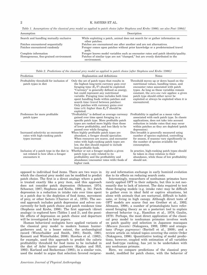
Table 1. Assumptions of the classical prey model as applied to patch choice [after Stephens and Krebs (1986); see also Post (1984)]

Assumption Description

Search and handling mutually exclusive While exploiting a patch, animal does not search for or gather information onother patches.

Patches encountered sequentially Patches are encountered one after another and are not alternatives.Patches encountered randomly Forager comes upon patches without prior knowledge or a predetermined travel

path.Complete information Forager knows model variables such as encounter rates and patch identity/quality.Homogeneous, fine-grained environment Patches of similar type are not ‘‘clumped,’’ but are evenly distributed in the

environment.

Table 2. Predictions of the classical prey model as applied to patch choice [after Stephens and Krebs (1986)]

Prediction Explanation and definitions Notes

Profitability threshold for inclusion ofpatch types in diet

Only the set of patch types that results inthe highest long-term currency gain overforaging time (En/T) should be exploited.‘‘Currency’’ is generally defined as energy,but could represent any nutritionalvariable. Foraging time includes both timespent handling foods within patches andsearch time (travel between patches).Only patches with currency gains overtime (e/h) higher than En/T should beexploited.

Threshold moves up or down based on thenutritional values, handling times, andencounter rates associated with patchtypes. As long as these variables remainconstant, the zero-one rule applies: a givenpatch type should either never beexploited or always be exploited when it isencountered.

Preference for more profitablepatch types

‘‘Profitability’’ is defined as average currencygained over time spent foraging in aspecific patch type. More profitable patchtypes are ranked more highly than thoseof lower profitability, and less likely to bepassed over while foraging.

Profitability is applied as a mean valueassociated with each patch type. In classicapplications, does not take into accountreduction in intake rates that may occurwithin patches as they are depleted (patchdepression).

Increased selectivity as encounterrates with high-ranking patchtypes increase

When highly profitable patch types areabundant, a forager should specialize.When resources are scarce, and encounterrates with high-ranking patch types arelow, the diet should expand to includeless-profitable foods.

Diet breadth is generally measured usingnumber of species exploited, controllingfor season, if seasons vary significantly inthe number of species available forconsumption.

Inclusion of a patch type in the diet isnot related to how often a foragerencounters it

Whether or not a forager exploits a givenpatch type is only related to itsprofitability and the profitability andabundance (encounter rates with) foods ofhigher rank.

In practice, high-ranking patch types shouldbe taken in close relation to theirabundance, while those of low profitabilityshould not.

2 K. SAYERS ET AL.

American Journal of Physical Anthropology

Himalayan gray langurs (Semnopithecus entellus) livingat a high altitude (3,000–4,000 m) site at LangtangNational Park, Nepal. The gray langur is a colobinemonkey possessing a large, multichambered stomachwith symbiotic gut microorganisms, which aid in thedigestion of high-fiber foods (Bauchop and Martucci,1968; Kay and Davies, 1994). Although colobines arepopularly described as ‘‘leaf-eating monkeys,’’ gray lan-gurs have an eclectic, generalist diet that varies season-ally (Koenig and Borries, 2001), and this is particularlytrue of Himalayan populations (Curtin, 1982; Sayers andNorconk, 2008). This provides an ample opportunity toinvestigate predictions of the classical prey model asthey pertain to behavioral shifts in response to changesin the abundance of foods. Field observations includedcontinuous recording of feeding bouts and between-patchtravel times, and laboratory work included standardnutritional analysis of langur foods. We apply a simplepatch choice version of the classical prey model withcorrections for search costs and use three nutritionalcurrencies [kcal, kcal with a flat correction for neutraldetergent fiber fermentation, and crude protein (CP)].Because the classical prey model has not been fullyapplied to any nonhuman primate, we feel it is appropri-ate to begin with this simple, but potentially robust,model before moving to a more complex one with addedconstraints or nutritional variables (Grether et al., 1992;Kaplan and Hill, 1992).

METHODS

Study site and subjects

Langtang National Park is located in north-centralNepal on the Tibetan border, and the Langtang Valleybetween Ghore Tabela (3,033 m) and Langtang village(3,480 m) was our primary area of observation. Severalvegetation types are present, all temperate or alpine,with different woody species characterizing each habitattype/elevation. On the north side of Langtang Khola(River), broadleaf trees and shrubs make up much of thewoody plant cover, whereas the south side is largely co-niferous forest. Other habitat types include cultivatedand noncultivated fields, rockslides, and cliffs. A smallhuman population is found at the village of Langtang.The climate is highly seasonal, with cold winters thatinclude periodic snow cover, and a mild summer mon-soon [see Sayers and Norconk (2008) for further details].All observations reported here involve a single troop of

Himalayan langurs. Members of this troop, once con-tacted, could generally be approached within 10 m,although this was in some cases not possible when themonkeys utilized cliff habitats or when rain/snow ren-dered human climbing difficult. Group size ranged from27 to 33 individuals, with a modal number of 3 adultmales and 10 adult females.

Behavioral observations

All behavioral observations were dictated into an audiorecorder between December 2002 and December 2003 andsubsequently transcribed. A different focal individual waschosen for each sample day (n 5 53), and data were col-lected on each food patch that was observed to be enteredby this individual. The formal definition of a patch isgiven below. Focal individuals were rotated among nona-dults (‘‘juveniles’’), adult females, and adult males.Because the length of time in which individuals could be

followed varied extensively based on topography andweather, feeding data were collected from other individu-als chosen at random whenever the focal animal was notvisible. This occurred on most sample days. Wheneverpossible, individual identification was recorded.When a target individual was observed to enter, or

was already feeding in, a food patch, the following datawere dictated into the recorder: food species, plant partingested, the time and size of each bite, within-patchtravel, and time of patch departure. Bite size refers tothe number of food items (leaves, fruit, etc.) put into themouth, and when number could not be determined, theaverage number of items per bite for that patch waslater substituted. Periods when ingestion could not beobserved were considered missing time and discarded(after Grether et al., 1992). When the focal individualleft a patch, it was followed, whenever possible, until itentered another food patch, and recording ceased onlywhen the individual stopped feeding or moving. Whennecessary, observations were aided by binoculars, or,rarely, a spotting scope. These data allow estimation ofintake over time in a second-by-second fashion for eachpatch or patch type, as well as average travel timebetween food patches. In total, 402 langur patches wererecorded (over 53 days distributed throughout a year)that included age-sex data and foods in which all nutri-tional analyses have been performed. Ninety-seven (97)between-patch travel times were estimated. Sample sizeswere not equally distributed over the year, as weatherconditions and the ranging behavior of the monkeysdetermined the likelihood and duration of contact withthe troop. Seasonal (defined below) patch numbers/sam-ple days were as follows: late winter (15/8), spring (71/9),late monsoon (9/2), fall 1 (35/5), fall 2 (54/8), fall 3 (73/8),fall 4 (113/11), and early winter (32/2).Food types were collected and weighed wet, field dried,

and after laboratory drying. Laboratory drying was com-pleted at Peabody Museum, Harvard University. Plantidentifications were conducted by plant scientists at theCentral Department of Botany, Tribhuvan University,Kathmandu, Nepal.

Nutritional analysis and currenciesfor the model

Nutrient (CP, water soluble carbohydrate, lipids, andhemicellulose) and non-nutrient (cellulose, cutin, lignin,and tannins) analyses were conducted by KS on 55 Hi-malayan langur food types at the Nutritional EcologyLaboratory in the Department of Anthropology, PeabodyMuseum, Harvard University (after Conklin-Brittain etal., 1998; Wrangham et al., 1998). CP was determinedusing the Kjeldahl procedure for total nitrogen and mul-tiplying by 6.25 (Pierce et al., 1958) instead of using the4.3 conversion factor (Conklin-Brittain et al., 1999; Nor-conk and Conklin-Brittain, 2004).The detergent system of fiber analysis (Goering and

Van Soest, 1970) as modified by Robertson and van Soest(1980) was used to determine the neutral-detergent, ortotal cell wall fraction (NDF) that includes hemicellulose(HC), cellulose (Cs), sulfuric acid lignin (Ls), and cutin.Total ash, an estimate of overall mineral content, wasmeasured in accordance with Williams (1984). Lipid con-tent was measured using petroleum ether extraction for4 days at room temperature, a modification of themethod of the Association of Official Analytical Chemists(Williams, 1984). Free simple sugars (FSS) (formerly

3HIMALAYAN LANGURS AND OFT


referred to as water soluble carbohydrates, Conklin-Brit-tain et al., 1998) were estimated using a phenol/sulfuricacid calorimetric assay developed by Dubois and col-leagues (1956) and modified by Strickland and Parsons(1972), with sucrose as the standard. Total nonstructuralcarbohydrates (TNC) were calculated as follows: TNC 5100 2 % NDF 2 % lipids 2 % CP 2 % ash (Conklin-Brittain et al., 1998). The results of the analyses areused as a percentage of organic matter (OM), whichexcludes inorganic materials.Currencies for use in the foraging models include: (1)

zero-fermentation metabolizable energy (MEO, kcal/100 gOM) 5 (4 3 % TNC) 1 (4 3 % CP) 1 (9 3 % lipids), (2)high-fermentation metabolizable energy (MEH, kcal/100g OM) 5 MEO 1 (2.0 3 % NDF), and (3) CP (Conklin-Brittain et al., 2006; National Research Council, 2003).Energy is a convenient currency that is applicable in

many situations and has the added advantage thatsearch costs can also be reported in kilocalories.Although nutritional analyses of colobine foods thatinclude estimates of energetic value are rare, this vari-able has been suggested to be an important componentof food selection for some colobines (Dasilva, 1994), andHimalayan langurs live in a marginal environmentwhere energetic considerations are likely to be important(Sayers and Norconk, 2008). However, because of theforegut fermentation of colobine monkeys, they are likelyable to derive more energy from fibrous foods than issuggested by the standard MEO equation (Kay andDavies, 1994). Conklin-Brittain and colleagues (2006)calculated MEH in chimpanzees, which can digestapproximately half of the NDF in their diet throughhindgut fermentation, as MEH 5 MEO 1 (1.6 3 % NDF).Foregut fermenters, however, show greater apparentdigestibility of fiber than do hindgut fermenters(Edwards and Ullrey, 1999), with values of at least68.9% of NDF (National Research Council, 2003). There-fore, here, we use MEH 5 MEO 1 (2.0 3 % NDF) as aconservative correction to account for colobine fermenta-tion. There are likely to be problems with this ‘‘flat’’ cor-rection applied equally to all food types, as foods withdiffering nutritional characteristics may be assimilatedin differing fashions. However, at this point, very little isknown about the differences in assimilation of differentcolobine foods, other than a general preference for lower-fiber leaves over higher fiber leaves (Waterman andKool, 1994). We argue the ‘‘flat’’ correction is a reasona-ble starting point for the investigation of such questions.CP has long been considered to play a role in diet

choice for colobine monkeys (Milton, 1979; Wassermanand Chapman, 2003) and herbivores in general(Newman, 2007). Note from the above that CP is in itselfa component of ME calculations and the two measure-ments may be correlated. A number of workers havefound that a protein-to-fiber ratio is useful in predictingcolobine leaf choice (Milton, 1979) or even biomass(Chapman et al., 2002). The primary limitation to theuse of a ratio is that it is often unclear whether it is thenumerator or denominator, or both, that is driving foodselection, and thus we limit ourselves to CP in the forag-ing model.

Seasonal time periods and age-sex categories

Eight seasonal time periods are used in the tests ofmodel predictions. These were chosen on the basis ofsample sizes as well as phenology (Sayers and Norconk,

2008): late winter (late December–March), spring (April–May), monsoon (September), fall 1–4 (October and No-vember, divided into four 2-week samples), and earlywinter (early December). Ideally, encounter rates withpatch types (i.e., food abundance) and the profitability ofeach patch type (i.e., nutritional quality) should remainconstant throughout each time period in which themodel is applied.Age-sex categories are modified from Bishop (1975)

and include adult males, adult females, and juveniles(nonadults). In some model applications, only data froma single adult male is considered. This single male wasalso the alpha male, which should reduce dominanceeffects on diet selection.

Definition of a patch

In foraging theory, a patch is usually defined as anarea of food concentration separated from other patchesby areas with little or no food. Sequential encounteroccurs when patches are met one after another (Table 1).Simultaneous encounter, a deviation from the assump-tions of the model considered here, occurs when patchesare met more-or-less at the same time (Stephens andKrebs, 1986). For this study, each tree, shrub, cultivatedfield or herb clump is generally considered a separatepatch (see Astrom et al., 1990). There are, however,some situations that are somewhat ambiguous; for exam-ple, when multiple plants grow contiguously or morethan one food type is found on a single plant. For thisreason, we give the following formal definition of apatch:

1. A patch contains only one food type. A food type isthe unit that is handled at one time. For example, if amonkey picks fruit from a tree and consumes both theflesh and seeds, this is considered one food type. If,however, a monkey eats fruit from a tree and thenswitches to eating leaves on the same tree, and theyare not handled or consumed together, they are con-sidered here as two food types from two patchesencountered simultaneously. This ‘‘one food type rule’’is used for analytical convenience and ease of inter-pretation; allowance for more than one food typewithin a patch will be considered elsewhere.

2. The travel time to a food source (e.g. a plant) mustexceed the average between-item ingestion times fromthe previous food source to qualify as being twopatches encountered sequentially. For example, ifleaves in one shrub are consumed at an average rateof one leaf (or one leaf clump) every 10 s, the traveltime to another shrub of the same species and foodtype must exceed 10 s to be considered a separatepatch.

3. In cases where travel time to a food source (e.g. aplant) does not exceed the average between-itemingestion time from the previous food source, andthey differ in species or food type, they are consideredhere as two patches encountered simultaneously.

Patch types as defined earlier were used for all calcula-tions performed in this work.

The model

Although there are a number of derivations of theclassical prey model, we choose a modified version thattreats patches as analogous to prey and include search

4 K. SAYERS ET AL.


costs (Schoener, 1974; Charnov, 1976; Paulissen, 1987;Schoener, 1987). The formula for the model is as follows:

En

T¼

PðkieiÞ � Cs

1þPkihi

ð1Þ

where En/T is the net energy (or other currency)acquired over time foraging, ki is the encounter ratewith patches of type i, ei is the mean energy (or othercurrency) acquired per patch of type i, hi is the meantime spent handling items in a patch of type i, and Cs isthe cost of searching for food (kilocalories per second).Encounter rates (ki) were determined by dividing the

number of patches of type i entered by total search time.Search time equals the average travel time betweenpatches for that season 3 total number of patches(counting only those encountered sequentially) for thatseason. Only patches where at least one bite of food wastaken were considered ‘‘encountered.’’ Although thismethod only gives information on patch types that areexploited, it does provide an estimate of encounter ratebased on actual animal observations and is the approachtaken in some of the more detailed tests of the classicalprey model (Paulissen, 1987). A preferable approachwould be to record, over time, every patch that enters aforager’s range of perception (e.g., within an arbitrary dis-tance radius), although this was not possible in the pres-ent study. Encounter rates are expressed as patches persecond of search time. The currency (ei) is expressed asthe mean kilocalories or grams OM (for CP) acquiredwhile exploiting a patch of type i, and handling time (hi) isexpressed as the average number of seconds spent exploit-ing a patch of type i. For example, if a patch type on aver-age yields 20 kcal per visit and is exploited an average of100 s per visit, the profitability of this patch type (ei/hi)would equal 0.2 kcal/s (12 kcal/min). These mean valuesare calculated using all recorded patches regardless of res-idence time, or whether the complete patch session wasrecorded. Once again, missing time, when ingestion move-ments could not be seen, was discarded and not used inthe calculation of ei or hi. Raw data concerning the abovevariables are given in the Appendix section.As much (though not all) between-patch travel in

Himalayan langurs occurs on the ground, search costs (Cs)were determined using a general equation for the mass-specific cost of terrestrial locomotion (Taylor et al., 1982):

Emetab

Mb¼ 10:7M�0:316

b 3vg ð2Þ

where vg is velocity in meters per second and Emetab

Mbhas

units of watts/kg, which were then converted to kilocalo-ries. Zero-speed costs are not included. The average veloc-ity was estimated at 1.25 m/s, considered a ‘‘comfortablewalking speed’’ for most primates (Steudel-Numbers, 2003,p. 257). Weights of adult males were estimated at 19.5 kg,adult females 16.1 kg, and juveniles as 12.1 kg ([3/4] theweight of adult females) (from Bishop, 1975). Search costsare not included when utilizing CP as currency.

Model predictions and statistics

Prediction 1: Quantitative estimation of profitabilitythreshold for dropping items from diet. For each of eightseasonal time periods, patch types were entered into

Equation 1 in the order of their profitability (MEO orMEH in mean kcal/second, CP in mean grams OM/sec-ond). Variables were entered into Eq. (1) with patchesfrom (1) only juveniles, (2) only adult females, (3) onlyadult males, and (4) only a single adult male. As eachpatch type is entered for an age-sex class and season,the calculated En/T reflects the average rate of gainwhile foraging. Only those patch types with averageprofitability (ei/hi) above the highest possible En/T (thethreshold value) are predicted to be included in the diet;all others should be rejected in favor of continued search.The proportion of the diet consisting of patch types withaverage profitability above the threshold (i.e., predictedin the optimal diet) and below the threshold (not pre-dicted) were quantified for each application. The percentcontribution of patch types in the diet was calculatedusing both OM (grams OM from patch type i/total gramsOM from all patch types) and time (seconds spent feed-ing on patch type i/seconds spent feeding on all patchtypes). The model predicts that patch types with profit-ability lower than the maximum possible En/T will notbe exploited, or, in the manner expressed here, willmake up 0% of the diet. A more direct test of the modelwould involve measuring the number of acceptances/rejections of patch types as they enter the range of ananimal’s perception, but, as noted earlier, it was not pos-sible to gather this data. Because the classical preymodel is designed to predict the behavior of a single for-ager and that the ‘‘optimal diet’’ may differ between indi-viduals, it is expected that the application using datafrom only a single adult male will most closely fit themodel (Krebs and McCleery, 1984).

Predictions 2–4 were tested using Spearman rankorder correlations.

Prediction 2: More profitable patch types will be prefer-red. Correlations were used to assess the relationshipbetween patch type profitability by MEO, MEH, and CPand percent contribution to annual diet by both OM andtime spent feeding. The latter is used as an indirect indi-cator of ‘‘preference.’’ To account for temporal effects infood availability, correlations were also performed for allseasonal time periods where �5 patch types were exploited.

Prediction 3: Higher encounter rates with profitable foodswill result in increased selectivity. The patch typesexploited by members of each age-sex class, and by oneindividual male, were divided into two categories, ‘‘high-ranking’’ (top half) or ‘‘low-ranking,’’ (bottom half) basedon their profitability across all patches and seasons byMEO, MEH, or CP. This method was used to estimate ingeneral how many ‘‘rich’’ versus ‘‘poor’’ patch types wereavailable in a given season. Encounter rates with high-ranking foods were then correlated with the number ofpatch types (species and plant part) and food parts(plant part only) taken during seasonal time periods. Forthe latter condition, plant part categories included (1)deciduous and herbaceous leaves, (2) evergreen leaves,(3) dormant leaf buds, (4) fruit and seeds, (5) soft under-ground storage organs, (6) hard or woody undergroundstorage organs, (7) bark, and (8) flowers. The classicalprey model, in general, predicts a negative correlationbetween the abundance of (encounter rate with) high-ranking foods and the number of patch types or plantparts included in the diet. However, this prediction maynot hold if comparisons are made across seasons that dif-



fer markedly in the number of food types available forconsumption [as in the Himalaya, Sayers and Norconket al. (2008)]. For this reason, data were also qualita-tively inspected to see if low-ranking foods available overmuch of the year were taken only when encounter rateswith high-ranking foods were low, as predicted by the model.

Prediction 4: Selectivity is not dependent on encounterrates with low-ranking patch types. The encounter rateswith low-ranking patch types and high-ranking patchtypes were correlated with the percent of the diet madeup of low-ranking foods by OM and time. The model pre-dicts no correlation between abundance of low-rankingpatch types and their dietary contribution, but a nega-tive correlation between the encounter rates with high-ranking patch types and the percentage of the dietinvolving low-ranking foods.

Comparison of nutritional currencies. For each age-sexclass, conformation of langur behavior to model predic-tions was examined under MEO, MEH, and CP. For eachprediction, currencies were given a rank of 1–3, with1 5 closest to model predictions and 3 5 furthest frommodel predictions. For all the predictions discussedbelow, situations where rankings differed based on quan-tification method (e.g., OM versus time estimates ofdietary contribution) were classed as ties. When tiesoccurred, rankings for all three currencies equaled sixwhen summed. In cases where langur behavior differedquantitatively from model predictions, under all threecurrencies, they were ranked as ties. Overall rankings ofcurrencies were based on averages across all predictionsfor each age-sex class.For the quantitative threshold for dropping items from

the diet, the percentage of foods in the predicted optimaldiet was compared for each season and currency. Thiswas performed both with and without the inclusion ofsearch costs. The currency that included the highest per-centage of diet in the predicted optimal set by OM andtime spent feeding was given a rank of 1.For the prediction that animals will prefer profitable

foods, the strength of correlation between preference andpatch type profitability was examined for each currency.Preference was ascertained by annual correlationsbetween dietary contribution, by both OM and time, andthe profitability of patch types (average caloric or proteingain over time) based on each the three currencies. Thecurrency yielding the strongest positive correlationbetween dietary contribution and profitability was giventhe rank of 1. When ties occurred for annual contribu-tion, currencies were ranked for all seasons with �5feeding sessions and overall rankings were based onaverages from this sample.For the prediction that inclusion in the diet is inde-

pendent of encounter rate, two measures were examined:(1) the strength of the predicted negative correlationbetween encounter rates with high-ranking patch typesand dietary contribution (by OM and time) of low-rank-ing foods, and (2) the predicted noncorrelation betweenencounter rates with low-ranking foods and their dietaryinclusion (again, by both OM and time). The currencywith the strongest correspondence to these predictionswas given a rank of 1, with the following stipulations:for both (1) and (2), discrepancies between OM and timeestimates were again considered ties, and for the latter,currencies were considered ties if there was not a signifi-cant positive correlation among them. The rankings forboth (1) and (2) were then averaged.

Deviations from model assumptions. To quantify season-specific deviations from assumptions, we identified cer-tain patch types that were exploited in a manner some-what incongruent with the scenario depicted by themodel (Table 1) by a single adult male. Herbaceous vege-tation was considered the most-likely patch type cate-gory to deviate from the ‘‘exclusivity of search and han-dling’’ assumption. At Langtang, multiple herb specieswere often interspersed on the ground, providing situa-tions where foragers, while feeding on one species, couldevaluate (or ‘‘search’’ for) others. Large patch types (i.e.,all excepting shrubs, herbs, and climbers) were consid-ered more likely to deviate from the random encounterassumption. Trees of favored species and potato fields,for example, were revisited and in some cases, especiallythe latter, their locations appeared to influence grouptravel paths. It is presumed here that animals are lesslikely to remember the specific locations of individualpatches of smaller size, such as shrubs, herbs, orclimbers (but see Menzel, 1991). The seasonal percen-tages of definite simultaneous encounters, where ani-mals exploited �1 food type more-or-less at the sametime (see ‘‘definition of a patch,’’ above), were recorded.Greater numbers of patch types exploited in a seasonwere viewed as rendering the ‘‘complete information’’assumption more unlikely. The model assumes that ani-mals have knowledge of variables such as the encounterrate with a given patch type or its profitability, but inreality foragers must acquire such information throughexperience before converging on a ‘‘steady state’’ patternof behavior (Staddon, 1983, p. 156). Psychological worksuggests that animals can better remember food charac-teristics when there are fewer of them; that is, whenthere is less ‘‘interference’’ (p. 262). In addition, thenumber of woody habitats exploited per season wasnoted, with the assumption that feeding within one habi-tat is more likely to approximate the assumption of afine-grained environment than multiple habitats.All statistical tests are two-tailed with P \ 0.05 and

were performed in SPSS 13.0, SPSS 16.0, and Sigmaplot.

RESULTS

Quantitative estimation of profitability thresholdfor dropping items from diet

An example of patch type ranking and profitabilitythreshold calculation [from Eq. (1)] is given in Table 3for a single adult male using kilocalories (MEO) as cur-rency. The model predicts that all exploited patch typesshould be above the En/T threshold (i.e., on Table 3, allpatch types would be in bold face). Langurs, includingthis adult male, consistently exploited patch types thatwere, on average, poorer than the calculated profitabilitythreshold. Patch types with average profitability belowthe thresholds, however, were generally taken only insmall amounts, with just a few exceptions. The primaryexception involves the mature leaves of Cotoneaster frig-idus, which in fall 1 drops the overall foraging efficiencyto a third of the optimal diet. Over all age-sex classes,the monkeys included patch types beneath the profitabil-ity threshold in 23/24 (95.8%) applications of the model(considering only seasons where n � 5 feeding sessions),and this rate of failure was the same regardless of thenutritional currency used (Figs. 1–4). The predicted opti-mal diet differed based on currency used in 16/24(66.7%) of model applications. Although MEO and MEH

differed from one another in only 7/24 (29.2%) of cases,

6 K. SAYERS ET AL.


the CP predicted diet differed from MEO and MEH in16/24 (66.7%) and 14/24 (58.3%) of applications, respectively.The diet of a single adult male, which resembles the

pooled age-sex results, shows seasonal differences in theextent to which the model could account for observedfeeding behavior (see Fig. 4). The model performed bestin spring, where, under all three currencies, only onefood type was predicted in the optimal diet. This item,consisting of clusters of Zanthoxylum nepalense youngleaf and flowers (handled and ingested together), madeup 86.3% of dietary OM and represented 73.6% of forag-ing time. For other seasons, however, the model failed tovarying degrees based on the currency entered into Eq.(1) and/or the method used to quantify diet. Most strik-ingly, under both energetic and CP currencies, this malespent considerable amounts of time exploiting patchtypes not predicted in the optimal diet.

More profitable patch types will be preferred

The model predicts a positive correlation betweenaverage patch profitability (ei/hi) and exploitation. Forgrouped age-sex classes (juveniles, adult females, andadult males), contribution of food types to annual diet bypercentage OM was positively related to MEO, MEH, and

CP profitability (Table 4). Conversely, annual percentfeeding time was not significantly correlated with profit-ability with the exception of MEO in the adult male cate-gory. Seasonal contribution to diet by percentage OMwas, in general, positively correlated with profitabilityunder all three currencies. Significant positive seasonalrelationships between feeding time and profitability,however, were the exception rather than the rule.For the single adult male, annual OM contribution

was positively related to profitability under all three cur-rencies (Table 4). Correlation coefficients between annualfeeding time and profitability were also positive, but notstatistically significant. Within seasons, significant posi-tive relationships were detected between OM contribu-tion and MEO and/or MEH profitability. A significant pos-itive relationship between feeding time and MEO orMEH profitability was apparent in two of three seasons.CP profitability was not significantly correlated with sea-sonal percentages by either OM or feeding time.

Higher encounter rates with profitable foods willresult in increased selectivity

Under the model, diet breadth is expected to decreaseas food abundance increases. Contrary to expectations,

Table 3. Seasonal patch types, overall rate of gain [En/T, calculated from Eq. (1)], and dietary contribution (% organic matter [OM]and feeding time) for a single adult male

Season Patch type En/T (kcal/min) % of diet (OM) % of diet (time)

Spring Zanthoxylum nepalense YL/FL 1.617 86.3 73.6Rosa macrophylla YL 1.565 11.5 17.9Cotoneaster frigidus YL 1.471 2.2 8.6

Fall 1 Solanum tuberosum USO 15.356 85.5 21.8Caragana gerardiana seed 15.213 1.4 1.3Rumex nepalensis HL 14.648 2.3 2.9Cotoneaster frigidus ML 5.748 10.8 74.0

Fall 2 Solanum tuberosum USO 19.418 73.8 45.0Clematis montana ML 18.739 6.6 6.5Rumex nepalensis HL 18.488 0.9 1.3Hippophae rhamnoides ML 16.573 6.5 10.6Elsholtzia fruticosa FL 15.745 3.1 5.7Caragana gerardiana seed 15.532 0.5 1.4Theropogon pallidus HF 15.405 0.4 0.9Raphanus sativus HL 15.297 0.2 0.7Malva sp. HL 12.385 7.5 24.1Compositae HL 12.321 0.2 0.7Fagopyrum esculentum HL 12.308 0.0 0.1Hippophae rhamnoides UF 12.052 0.2 2.3Cotoneaster frigidus ML 11.967 0.1 0.8

Fall 4 Hippophae rhamnoides ML 3.173 9.1 2.7Caragana gerardiana seed 3.419 0.5 0.2Sorbus cuspidata RF 7.603 23.3 5.9Solanum tuberosum USO 8.281 44.1 45.4Cotoneaster frigidus RF 7.984 3.3 4.2Allium wallichii HF 7.957 0.2 0.4Cotoneaster frigidus ML 6.300 17.9 35.3Euphorbia sp. RF 6.190 1.2 3.3Cotoneaster acuminatus RF 6.143 0.3 1.1Berberis aristata RF 6.066 0.1 1.5

Early winter Hippophae rhamnoides ML 3.783 55.0 22.5Caragana gerardiana seed 4.202 20.4 29.6Aconogonum molle USO 4.010 6.1 11.8Cotoneaster frigidus RF 3.734 14.1 22.9Cotoneaster frigidus ML 3.618 3.4 9.2Cotoneaster frigidus LB 3.530 0.9 4.1

Patch types listed in order of their profitability with kilocalories over time (MEO) utilized as currency. En/T shows the rate of gain ifonly that patch type and those of greater profitability were taken; patch types included in the predicted optimal diet for each seasonare given in bold face. Only seasons with �5 feeding sessions are shown. YL, young leaf; ML, mature leaf; HL, herb leaf; RF, ripefruit; UF, unripe fruit; HF, herb fruit; LB, leaf bud; USO, underground storage organ.



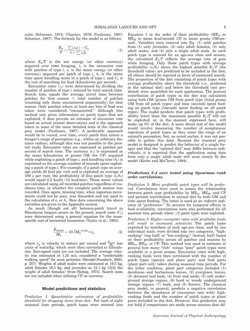
Fig. 1. The seasonal mean profitability of patch typesexploited (data points) and calculated En/T threshold for inclu-sion in diet (line) for juveniles under three different nutritionalcurrencies. For all seasons with n � 5 feeding sessions, the per-centage of feeding time spent on foods in the predicted set(above the threshold) is given at the top of the figure, with thepercentage organic matter (OM) of diet above the threshold inbrackets. 1A, zero-fermentation metabolizable energy (MEo) ascurrency; 1B, high-fermentation metabolizable energy (MEh) ascurrency; 1C, crude protein (CP) as currency.

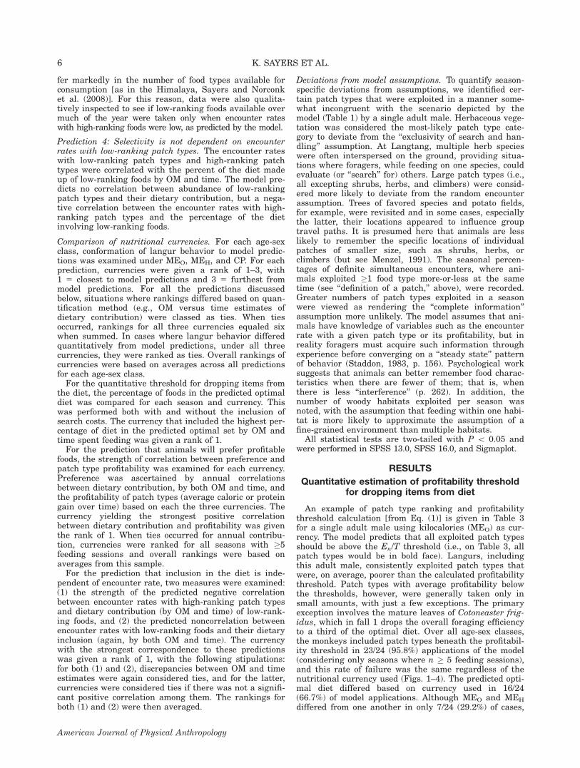
Fig. 2. The seasonal mean profitability of patch typesexploited and calculated En/T threshold for inclusion in diet foradult females under three different nutritional currencies. Thenotation and description are as in Figure 1.

8 K. SAYERS ET AL.


neither the number of patch types nor plant partsexploited by grouped age-sex classes or a single adultmale were significantly related to seasonal encounter

rates of high ranking foods under any currency (Table 5).This is likely related to the fact that many profitablefoods were available simultaneously in the fall seasons,

Fig. 3. The seasonal mean profitability of patch typesexploited and calculated En/T threshold for inclusion in diet foradult males under three different nutritional currencies. Thenotation and description are as in Figure 1.

Fig. 4. The seasonal mean profitability of patch typesexploited and calculated En/T threshold for inclusion in diet fora single adult male under three different nutritional currencies.The notation and description are as in Figure 1.



while in the winter and spring seasons there were fewerfood types of any kind available (Sayers and Norconk,2008).Nevertheless, qualitative inspection of data from all

age-sex classes (Appendix section) and nonseasonal foodssuggests that this prediction was partially supportedwhen food availability is considered. Certain food itemsthat were considered of low profitability under all cur-rencies, such as Gaultheria evergreen mature leaves andpetioles and Elsholtzia fruticosa woody roots, were avail-able throughout the year but taken almost exclusivelywhen encounter rates with high-ranking foods were low-est (late winter).

Selectivity is not dependent on encounter rateswith low-ranking patch types

The model predicts no correlation between encounterrates with low-ranking patch types and their inclusionin the diet. In addition, it predicts a negative correlationbetween encounter rates with high-ranking foods andthe proportion of the diet consisting of low-ranking foods.For grouped data, juvenile foraging behavior mostclearly ran counter to model predictions (Table 6).Encounter rates with low-ranking foods were positivelyrelated to feeding time on low-ranking foods irrespective

of currency, and encounter rates with high-ranking foodsdid not show a significant negative correlation with thecontribution of low-ranking foods by either OM or time.In fact, for juveniles, encounter rates with high-rankingfoods were less-closely related to dietary contributionthan low-ranking foods.The behavior of adult females was consistent with the

model under MEO (Table 6). Using this currency, encoun-ter rates with low-ranking foods were not significantlyrelated to the dietary contribution of low-ranking foods,whereas the encounter rates with high-ranking foodsshowed a strong positive relation to the contribution ofhigh-ranking foods by both OM and time. For adultmales, similar agreement with the model was detectedunder both MEO and MEH. For both adult sexes in thepooled data set, the utilization of CP as currency pro-vided slightly weaker conformation to model predictions,as low-ranking foods as described by this currency weretaken in closer proportion to their encounter rates.Results from a single adult male were generally con-

sistent with the model (Table 6). Seasonal encounterrate with low-ranking foods, under all three currencies,was not significantly related to percent contribution oflow-ranking foods. Also as predicted, a significant nega-tive relationship was detected between encounter ratewith high-ranking foods (under both MEO and CP) andOM contribution of low-ranking foods. Correlation coeffi-cients concerning encounter rates of high-ranking foodsand percentage of time feeding on low-ranking foodswere negative but not statistically significant.

Comparison of nutritional currencies

Data from grouped age-sex classes and a single adultmale most closely approximated classical prey model pre-dictions using MEO as currency (Table 7). However, forthe ‘‘threshold’’ prediction, search costs were onlyincluded in the models for MEO and MEH, and increas-ing search costs can result in a broader predicted diet(Lifjeld and Slagsvold, 1988). When search costs wereremoved, CP resulted in greatest conformation for pooledadult females, and MEO for juveniles, pooled adultmales, and a single adult male.

Deviations from model assumptions

All age-sex classes engaged in foraging behavior thatlikely resulted in deviations from model assumptions,e.g., 78 of 402 patches (19.4%) involved definite simulta-neous encounters. Recall that the model predicts thebehavior of a forager encountering patches sequentially(Table 1). For a single adult male, the lowest degree ofdeviation from model assumptions occurred in spring,and this was also the season in which the model wasmost successful in predicting diet (Table 8).

DISCUSSION

A likely reason that few primatologists have used OFTis that the assumptions and variables of its models havebeen questioned. Although these critiques in some casespossess merit, we argue that the drawbacks have beengreatly exaggerated (Table 9). Although the classicalprey model, for example, sidesteps a number of relevantparameters, such as the effects of variance and feeding

Table 4. Spearman rank order correlation coefficients betweencontribution to diet of patch types (by % organic matter [OM] or% feeding time) and patch type profitability by age-sex class and

season

% OM % Time

n MEO MEH CP MEO MEH CP

JJAnnual 23 0.77** 0.72** 0.67** 0.35 0.27 0.37Fall 2 9 0.85** 0.85** 0.88** 0.48 0.48 0.82**Fall 4 7 0.96** 0.96** 0.43 20.07 20.07 20.14

$$Annual 47 0.51** 0.54** 0.49** 20.06 20.06 0.00Late

winter7 0.21 0.25 0.50 20.68 20.64 20.21

Spring 11 0.56 0.62* 0.67* 0.36 0.36 0.54Fall 1 6 0.89* 0.89* 0.77 0.26 0.26 20.03Fall 2 12 0.83** 0.83** 0.49 0.69* 0.64* 0.29Fall 3 14 0.69** 0.66** 0.75** 20.10 20.22 20.01Fall 4 17 0.51* 0.57* 0.67** 20.03 20.01 0.25Early

winter9 0.50 0.57 0.63 0.27 0.30 0.45

##Annual 30 0.64** 0.63** 0.47** 0.36* 0.35 0.20Spring 6 1.00** 0.94** 0.83* 1.00** 0.94** 0.83*Fall 1 7 0.50 0.50 20.04 20.25 20.25 20.75Fall 2 14 0.49 0.42 0.08 0.24 0.14 20.02Fall 3 8 0.81* 0.81* 0.79* 0.62 0.62 0.60Fall 4 11 0.66* 0.70* 0.61* 20.01 0.02 0.04Early

winter6 0.77 0.83* 0.77 0.49 0.60 0.54

#Annual 24 0.66** 0.70** 0.53** 0.33 0.36 0.27Fall 2 13 0.78** 0.73** 0.46 0.59* 0.53 0.24Fall 4 10 0.55 0.64* 0.39 0.08 0.20 20.07Early

winter6 0.94** 1.00** 0.71 0.71 0.83* 0.49

Only seasons where �5 food types were taken are shown. JJ, alljuveniles; $$, all females; ##, all adult males; #, one adultmale; MEO, zero-fermentation metabolizable energy; MEH, high-fermentation metabolizable energy; CP, crude protein.* , significant at the 0.05 level; ** , significant at the 0.01 level.

10 K. SAYERS ET AL.


competition, it touches on the primary ones and could addsignificantly to our knowledge of primate feeding behav-ior. For example, a wealth of studies have demonstratedthe influence of travel time (search time) between fooditems or patches on the decisions animals make inregards to what foods to eat and when to leave a givenpatch [reviewed in Nonacs (2001) and Sih and Christen-sen (2001)]. Yet this seemingly critical variable, a stapleof even the most basic OFT models, has only rarely beenaddressed in primate feeding studies (e.g., Rapaport,1995, 1998; interpatch distance, Suarez, 2006). In anextensive review of tests, it has been noted that predic-tions from the classical prey and other optimal dietmodels are most often upheld in foragers that feed onimmobile prey (e.g., fruit and leaves), a category whichwould accommodate the diets of many primates. In addi-tion, the model appears to be fairly robust and often with-stands violations of some of its assumptions (Sih andChristensen, 2001). All models are by definition abstrac-tions of nature, and simpler and more generalized modelscan gain in power what they lack in precision.Although Himalayan langurs generally exploited patch

types not predicted by the classical prey model, in mostcases these were rare foods taken only sporadicallywithin a season. For example, Cotoneaster frigidus leafbuds were sometimes consumed in the fall, but not onevery occasion when foragers entered a tree of this

species. In this respect, such foods represent partial pref-erences. These are deviations from the zero-one rule,which states that foods should always be taken or neverbe taken when they are encountered, as long as environ-mental conditions remain constant (Stephens and Krebs,1986). Partial preferences have been observed in almostall tests of the model, both in laboratory and field (Sihand Christensen, 2001). There are a number of reasonsfor partial preferences, several of which are relevant tothis study (Table 10). Most of the patch types that wereexploited, but not predicted, were relatively rare foodswhose consumption could hypothetically be explained as,for example, cases of patch sampling or the obtaining ofrare nutrients.Several foods taken beneath the threshold, however,

were not merely ‘‘partial preferences,’’ but were routinelyand consistently exploited. The most striking exampleinvolves the mature leaves of Cotoneaster frigidus, anabundant woody plant. This was ranked first or secondby annual feeding time for all age-sex classes, and inscan samples taken concurrently represented the highestpercentage of feeding records over an annual cycle(Sayers and Norconk, 2008). In no case was this resourcepredicted to be a part of the optimal diet for any age-sexclass, season, or currency. One possibility is that ournutritional sample is not representative of the averagequality of Cotoneaster frigidus, or that some other qual-ity associated with this food type renders it a preferreditem. It is also likely that Himalayan langurs perceivetheir environment as poorer than suggested by the cal-culations used in this study; that is, in the context of themodel, the ‘‘thresholds’’ should be lower than thosedepicted on Figures 1–4. For example, increasing searchcosts result in a broader predicted diet, and it is likelythat the general equation used here (Taylor et al., 1982)underestimates them. The Himalayan environment ischaracterized by extreme changes in topography,whereas the langurs must negotiate during travel andwhich makes movement more costly than would beexpected in flatter terrain (Sprague, 2000). In a similarvein, underestimates of search time or overestimates ofthe encounter rates with high-ranking foods would alsoresult in a narrower predicted diet than actually wouldbe observed (Kaplan and Hill, 1992; Winterhalder et al.,1988). It is in this regard that nonrandom encountercould cause violations from model predictions. Revisitingpatches will result in an exaggerated estimate of encoun-ter rates and, if it is a high-ranking food, could result inan overly narrow predicted diet breadth. Potato fields,for example, were revisited in the fall months. It is alsoimportant to point out that when variation in patch prof-itability is low, the costs of moderate deviation from thepredicted optimal diet may be minor, although that wasnot the case with some nonpredicted patch types consid-ered here, such as Cotoneaster frigidus.

Table 5. Spearman rank order correlation coefficients between seasonal encounter rates with high-ranking patch types (khigh ) underthree currencies and the number of food types or plant parts included in the diet

khigh khigh khigh khigh

JJ MEO MEH CP $$ MEO MEH CP ## MEO MEH CP # MEO MEH CP

Food types n 5 5 0.31 0.31 20.15 n 5 8 0.17 0.17 0.17 n 5 6 0.75 0.75 0.75 n 5 5 0.70 0.70 0.10Plant parts 20.26 20.26 0.37 20.16 20.17 20.16 0.29 0.29 0.10 0.53 0.53 20.16

Shown are all seasons with �5 feeding sessions for that age sex-class; sample size reflects number of seasons that meet this criteria.

Table 6. Spearman rank order correlation coefficients betweenseasonal encounter rates with high or low-ranking patch typesunder three currencies and proportion of organic matter (OM)

and feeding (time) devoted to low-ranking patch types

khigh klow

MEO MEH CP MEO MEH CP

JJ (n 5 5)% low OM 20.20 20.20 20.20 0.60 0.60 0.80% low time 20.20 20.20 20.70 0.90* 0.90* 1.00**% high OM 0.20 0.20 0.20 20.60 20.60 20.80% high time 0.20 0.20 0.70 20.90* 20.90* 21.00**

$$ (n 5 8)% low OM 20.79* 20.69 20.79* 0.43 0.76* 0.76*% low time 20.83* 20.52 20.79* 0.10 0.62 0.62% high OM 0.79* 0.69 0.79* 20.43 20.76* 20.76*% high time 0.83* 0.52 0.79* 20.10 20.62 20.62

## (n 5 6)% low OM 20.83* 20.83* 20.89* 0.14 0.20 0.71% low time 20.94** 20.94** 20.54 0.26 0.43 0.94**% high OM 0.83* 0.83* 0.89* 20.14 20.20 20.71% high time 0.94* 0.94* 0.54 20.26 20.43 20.94**

# (n 5 5)% low OM 21.00** 20.70 20.90** 0.00 0.30 20.70% low time 20.70 20.30 20.70 0.30 0.70 20.10% high OM 1.00** 0.70 0.90* 0.00 20.30 0.70% high time 0.70 0.30 0.70 20.30 20.70 0.10

* significant at the 0.05 level.** significant at the 0.01 level.



Other predictions of the model were generally qualita-tively or quantitatively upheld. Strong positive correla-tions were detected between patch type profitability andOM contribution to diet, whereas correlations betweenprofitability and feeding time were generally positive butweaker. This suggests that ‘‘profitability’’ as defined inthe classical prey model—but not necessarily as perceivedby the animals—is driven largely by intake rate, at leastwith regards to the Himalayan langur data set (see alsoSchulke et al., 2006). Foods of low profitability that wereavailable over the entire year were generally taken onlywhen encounter rates with profitable patch types werelowest. With the exception of juveniles, high-rankingfoods were taken in close relation to their abundance,while low-ranking foods were not. The deviation of juve-niles in this respect may be related to dominance effects,whereas high-ranking patches are disproportionatelyunavailable to them, or simply reflect that they are in aprocess of learning to forage efficiently (Pulliam, 1981).In general, langur behavior was closest to that pre-

dicted by the model using a standard energetic currency(MEO), although CP performed slightly better for groupedadult females when search costs were removed. Thesefindings run counter to some of the colobine literature,which argues for the primacy of CP in colobine food selec-tion. Wasserman and Chapman (2003), for example, foundno correlation between the energy content of food and for-aging effort, and a positive relationship between protein-to-fiber content and foraging effort, in red colobus (Proco-lobus badius) and guerezas (Colobus guereza) at Kibale,Uganda. In addition, they found that estimates of energyconsumption were higher than estimates of expenditurefor these monkeys and suggested that energy was of minorimportance. Although this certainly may be the case, wedo not accept their conclusion that these results demon-strate ‘‘the importance of protein over other nutritionalcharacters’’ (p. 657) or eliminate energetic considerations

altogether. Our reasons include (1) Wasserman and Chap-man looked only at the protein-to-fiber ratio, not CP alone,(2) in their calculations of energy consumption, intakerates for plant parts were not estimated directly, buttaken from studies of howler monkeys, (3) they assumedthat surplus energy is unnecessary, an unlikely scenarioin a stochastic environment (Stephens and Krebs, 1986),and (4) in any event, they provided no evidence to suggestthat CP is a limiting variable (Oftedal et al., 1991).Although protein is generally positively related, and di-etary fiber negatively related, to food selection in colo-bines, it is still an open question as to the relative im-portance of each of these variables. Fewer studies stillhave examined calories or intake rate, again making itdifficult to ascertain their general importance to colo-bine food selection. In this study, the predicted protein-maximizing and energy-maximizing diets generally(67% of applications) either differed only by one patchtype, or were identical.Contrary to expectations, metabolizable energy with a

correction for fermentation (MEH) did not unilaterallyoutperform the energetic currency without this correc-tion (MEO). Undoubtedly, being able to ferment higheramounts of fiber than other primates influences colobinefood choice, and leaves (stereotypically a high-fiber food)make up a significant proportion of the diet at moststudy sites (Kirkpatrick, 1999). Nonetheless, colobineshave consistently shown a preference for lower-fiber overhigher fiber leaves (Davies et al., 1988; Fashing et al.,2007). One interpretation of this is that fiber exerts a‘‘sliding scale’’ on colobine food preference. At low levels,fiber may be nearly completely digested, while at highlevels fiber will subtract from food value either throughincomplete digestion, an increase in gut retention time,or the overproduction of volatile fatty acids which couldalter fore-stomach pH (Lambert, 1998). Unfortunately,few data currently exist to test this hypothesis or to

Table 7. Comparison of results from the three currencies (MEO, MEH, and CP) utilized here in relation to the classical prey model

JJ $$ ## #

MEO MEH CP MEO MEH CP MEO MEH CP MEO MEH CP

Threshold 1 2.5 2.5 1 2 3 1.5 1.5 3 1 2.5 2.5Profitability – – – 2.5 2.5 1 1 2 3 2 1 3Increased selectivity – – – – – – – – – – – –Independence – – – 1.5 3 1.5 – – – 1.5 3 1.5Overall � � * � �

1, closest to model predictions and 3, furthest from model predictions. Blank cells represent ties across all currencies and check-marks (�) indicate the currency to which the model best conforms over all predictions. An asterisk (*) indicates the currency, if differentfrom above, that conformed best to model predictions when search costs were removed from MEO and MEH threshold calculations.

Table 8. Seasonal comparisons of likely deviation and compliance with model assumptions compared with success of the model inpredicting diet for a single adult male

Assumption Measure of deviation Spring Fall 1 Fall 2 Fall 4 Early winter

Search and handling mutually exclusive % herb 0 25.0 40.0 3.8 0Sequential encounter % simultaneous 0 25.0 80.0 15.4 22.2Random encounter % trees and cultivated fieldsa 14.3 62.5 40.0 80.8 66.7Complete information # food types 3 4 13 10 6Homogeneous, fine-grained environment # woody habitat types 1 2 1 2 2Least deviation from model assumptions �Highest percentage of diet predicted �

a In other words, large patch types, which do not include herbaceous plants, shrubs, or climbers. Justification in text.

12 K. SAYERS ET AL.


develop a more specific energetic currency for colobinemonkeys that includes variables such as item-specificassimilation (National Research Council, 2003). Elucidat-ing such factors should be one long-term goal for applica-tions of OFT to primates.Schoener (1987) noted several potential problems for

applying the classical prey model to patch choice, as per-formed here. One potential problem is that patches (suchas trees in this study) are less likely to be encounteredrandomly than individual prey items (such as a solitarygrasshopper) and can result in departure from modelpredictions. Another is that patches can be depleted anda forager may alter the profitability of a patch whileexploiting it. In this study, all patch types were assigneda mean value with no account taken of decreases inintake rate over time (patch depression). In other words,the patch type approach is more likely to result in devia-tions from the assumptions of the prey model than the

standard usage, but modifications can be incorporated insituations where patch depression is found to be impor-tant (Stephens and Krebs, 1986).In a wide-ranging review, Sih and Christensen (2001)

noted that the classical prey model has proven to bequite robust (even in patch choice applications) and oftenwithstands deviations from the assumptions of themodel. In this study, however, the model performed bestin spring, when fewer of these assumptions wereviolated and the animals were ‘‘playing the same gameas the model’’ (Stephens and Krebs, 1986, p. 204).Future applications of OFT to nonhuman primatesshould also attempt to determine which assumptions arebeing violated and its effects on model performance. Theresults given here suggest that such violations should beexamined, but need not discourage primatologists fromutilizing this powerful body of theory.

Table 9. Criticisms of classical OFT models

Criticism Explanation Comments

Primate diets are too complex from anutritional standpoint to beaccounted for by maximizing onevariable such as energy or protein(Glander, 1981, p. 157–158; Milton,1979; Richard, 1985).

Many animals face the problem of balancingcritical nutrients, toxins and digestioninhibitors, rendering classical OFT modelsinapplicable.

In many cases, one variable may besufficient to describe the general feedingpatterns of a given animal.a Someprimates may be able to detoxify certaincompounds or simply avoid plantscontaining them (Waterman and Kool,1994). At a reductionist level, toxins ordigestion inhibitors could simply besubtracted from overall food value, e.g.,total energy yield minus the energyexpended in detoxification or digestion(see Newman, 2007).

Classical OFT models assume a‘‘fine-grained environment’’ whereresources are evenly distributedand encountered in proportion totheir abundance in theenvironment. This in unlikely inmost primate habitats (Post, 1984).

Many animals actually inhabit a ‘‘coarse-grained environment’’ where theencounter rate with a given resourcechanges as they enter different parts oftheir range.

If sample sizes allow, OFT models such asthe classical prey model can be appliedseparately to different parts of theenvironment that have variable resourceabundances (Stephens and Krebs, 1986).Little evidence exists to suggest thatprimates deviate from this assumptionmore than other vertebrates to whichOFT models have been applied.

Maximization models fall prey to a‘‘fast-food fallacy,’’ predicting ‘‘dietsthat are quickly consumed but wellbelow the animal’s consumptioncapacity for foods and theircomponents, including energy’’(Altmann, 1998, p. 157–158).

Altmann (1998) illustrates with thehypothetical example of an animal thathas met its nutrient requirements for theday and then feeds on the most profitablefood type until it can no longer be eaten(e.g., it is rare in the environment). Wouldnot a rate-maximizing forager then refuseto feed on the second-most-profitablefood, as this would lower average intakerate?

In the classical prey model, the decisionvariable is whether or not to exploit a foodtype when encountered. It does notpredict time spent feeding; it is generallyassumed that animals will forage whenthey are hungry. In the hypotheticalexample, the encounter rate with the mostprofitable food type is low or has droppedto zero, and the diet would be predicted toinclude or expand to include the second-most-profitable food type.b

Classical OFT models are simplisticand do not account for all of thevariables that influence feedingbehavior (see Janson and Vogel,2006).

Variance in prey quantity or quality, hunger,predator avoidance, feeding competition,etc. are not considered in classical OFTmodels (Mangel and Clark, 1988; Houstonand McNamara, 1999; Caraco, 1981; Clarkand Mangel, 2000; Giraldeau and Caraco,2000).

Simple modifications on the classical OFTmodels address some of theseshortcomings. Nonetheless, the simplerthe biological model, and the more easilyit can be applied across taxa, the moreheuristic value it garners (Stephens et al.,2007).

a For example, energy shortfall as yearlings was found to account for 96% of variability in fecundity and 81% in reproductivesuccess for yellow baboon (Papio cynocephalus) females (Altmann, 1998). Although it is possible that energy alone would make areasonable currency for maximization in yellow baboons, Altmann does not make this contention. Also, maximizing one nutrientmay maximize many if they are correlated between food types (Glander, 1981; Stephens and Krebs, 1986).b The fast-food fallacy is a valid objection within models which assume that an animal can cease foraging as long as its minimumrequirements for the day are met. This is not an assumption of the classical prey model. In addition, OFT applications generallyexamine many foraging decisions simultaneously (maximizing long-term intake rate), again a scenario to which the fast-food fallacydoes not apply (Altmann, 1998; Stephens and Krebs, 1986).



Table 10. Potential causes of partial preferences, with application to the present study

Cause of partial preferences DescriptionRelevance to present study,

and other notes

Discrimination errors (Krebsand McCleery, 1984)

Different food types may be confused by theforager. Also, the extent to which thetaxonomy of food types used byresearchers (e.g., biological species andplant part) corresponds to that used bythe subjects is little known (see Menzel,1997).

In late winter at Langtang, deciduousplants are largely or completely devoidof leaves, and discriminating betweencertain types of bark or woody rootsmay be difficult. The same may applyto plant parts of differing specieswithin the same genera. However, thisis not likely to be a major cause ofpartial preferences, and studies haveshown that primates’ knowledge oftheir habitat can be substantial(Janson and Byrne, 2007; Menzel,1991, 1997).

Long-term learning (Krebs andMcCleery, 1984)

Accurate estimate of model variables mayonly be possible after many days ofexposure to similar conditions.

In highly seasonal habitats such asLangtang, conditions may change sorapidly that estimates of patch typeabundance or quality are one-stepbehind the environment, in a cognitiveanalogue of the ‘‘Red Queen’shypothesis’’ (see Kamil, 1983; VanValen, 1973).

Inherent variation in theanimal (Krebs and McCleery,1984)

Changes in the internal clock of a foragermay cause deviations from modelpredictions.

Unknown

Runs of bad luck (Krebs andMcCleery, 1984)

If the animal uses a short-term rule todetermine encounter rates, habitat qualitymay be underestimated after repeatedexposure to unprofitable foods.

Unknown

Simultaneous encounters(Engen and Stenseth, 1984;Krebs and McCleery, 1984)

Food items or patches are encountered atthe same time rather than sequentially.

A minimum of 19.4% of Himalayanlangur feeding sessions involvedundoubted simultaneous encounters.a

The model performed best in spring,when the lowest percentage ofsimultaneous encounters was recorded.

Averaging across individuals(Krebs and McCleery, 1984)

Model is designed to predict the behavior ofa single individual.

While likely a major reason for partialpreferences in the pooled age-sexcategories, partial preferences werealso noted for a single adult male.

Nutritional requirements andanti-feedant avoidance(Westoby, 1978)

Animal may take variable amounts of foodswith low e/h that are high in certainmacronutrients or minerals, or take onlylimited amounts of foods with qualitativeor quantitative plant defenses (e.g.,Fashing et al., 2007).

In most cases, no simple nutritionalrationale has yet been found for thosevariables for which we have data,including crude protein, free simplesugars, lipids, fiber fractions, andcondensed and hydrolizable tannins. Ithas been noted that high-starch dietsfed to captive primates, in particularforegut fermenters like colobines, canlead to excessive fermentation,stomach problems, and in extremecases even death (National ResearchCouncil, 2003). This may be a possibleexplanation for the expansion of thediet beyond potatoes in the fallapplications, when this resource was inmany cases the only patch typepredicted.b Although mineral analyseshave not yet been completed, thelangurs were observed licking rocks,possibly for sodium (Sayers andNorconk, 2008).

Differential predation dangerassociated with differingpatch types (Brown andKotler, 2007)

A patch with highly profitable food may beunderexploited if a forager is moreexposed to predators while feeding in it.

While feeding in potato fields, Himalayanlangurs were exposed to potentialaerial predators and also to localfarmers wielding sling-shots andstones (Brown and Kotler, 2007).

14 K. SAYERS ET AL.


Even simple models may have relevance to nonhumanprimate foraging behavior (Barton and Whiten, 1994).Although students of primate diet argue for approachesof greater and greater complexity (Felton et al., 2009), itis possible, and perhaps likely, that quantifying only sev-eral key variables from foraging theory (e.g., energy orprotein gain, handling time, and travel time) would besufficient to explain much of the variance in primatefeeding behavior. In this study, the classical prey modelwas applied to seasonal time periods from weeks tomonths in length, and it is probable that at study siteswhere a single individual could be followed for entiredays, the model could be doubly informative. Given thetemporal and spatial heterogeneity of primate habitats,we would suggest applying the model freshly on a weeklyor even daily basis to individual primates and habitattypes if sample sizes allow. Although not applied here,recent game-theory applications attempting to predictthe behavior of social foragers appear to be especiallyrelevant to group-living primates and hopefully will gen-erate enthusiasm among primate researchers (Giraldeauand Caraco, 2000; di Bitetti and Janson, 2001). Unfortu-nately, there are no social models as general as thosefrom classical foraging theory, at least pertaining to dietchoice. To date, the classical prey model has proven to beinformative in animals as diverse as invertebrates andhuman hunter-gatherers (Stephens and Krebs, 1986; Sihand Christensen, 2001), and it is hoped that this studywill encourage further applications of patch choice andexploitation models to other primates.

ACKNOWLEDGMENTS

Ram Rimal, Ranger Ming Mav Chhewang Tamang,and the Langtang National Park staff provided consider-

able assistance. Achyut Ahdikari, Nina Jablonski,Mukesh Chalise, Daniel Taylor-Ide, Robert Fleming, Jr.,Himalayan Glacier Trekking, Cemat Water Lab, andDindu Lama and family helped with multiple phases ofthis project. Owen Lovejoy, Richard Meindl, CharlesMenzel, and three anonymous reviewers provided criticalanalysis of earlier versions of the paper. The researchwas conducted in conjunction with the Nepal Ministry ofForests and Soil Conservation and Department ofNational Parks and Wildlife Conservation.

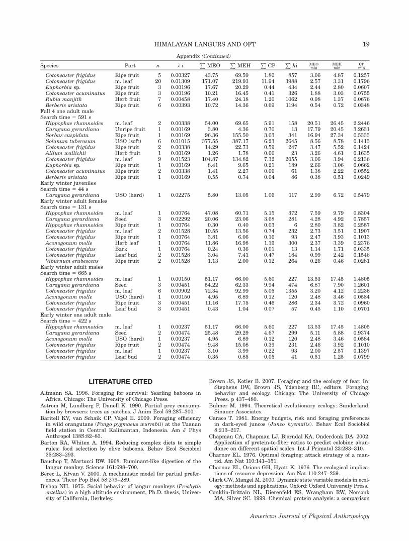
APPENDIX

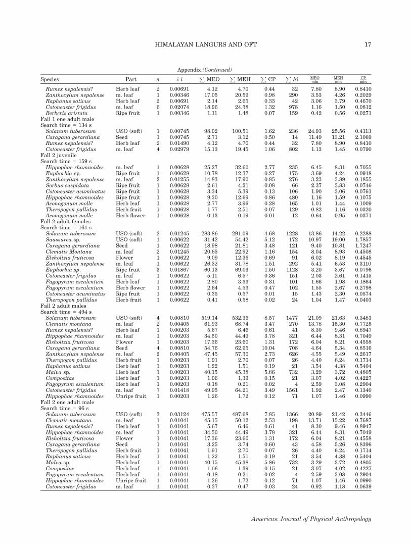
Variables used in Eq. (1) to estimate the profitabil-ity threshold for dropping items from the diet,arranged by season, age-sex classification, and plantpart. Encounter rates (ki) are given in patches (n) persecond of search time (search time 5 total estimatedtravel time between patches for the sample). Handlingtimes (hi) are given in seconds. For the three alterna-tive currencies, zero-fermentation metabolizableenergy (MEO) and high-fermentation metabolizableenergy (MEH) are given in kilocalories and crude pro-tein (CP) in grams organic matter. Profitability is pre-sented as currency per minute over all patches forthat food type and season [(currency/hi) 3 60]. Cur-rency and handling times were entered into Eq. (1)as mean values per patch (e.g.,

Phi/n). Food types for

each season and age-sex class are listed in order ofMEO profitability. Abbreviations: m. leaf, mature leaf;y. leaf, young leaf; USO (hard), underground storageorgan with woody texture; USO (soft), other textures.Fruits include both pulp and seeds unless notedotherwise.

Table 10. (Continued)

Cause of partial preferences DescriptionRelevance to present study,

and other notes

Sampling (Lima, 1984) Foragers may take small amounts of foodsto gain information about them, which isa deviation from the ‘‘completeinformation’’ assumption.c

Himalayan langurs were observed taste-testing Sorbus cuspidata fruit beforeacceptance or rejection.d

Local but not globalomniscience (Berec andKrivan, 2000)

The classical prey model presumes thatanimals are ‘‘globally omniscient,’’ andknow encounter rates with food items orpatches within the entire area that theyrange in for the period the model isapplied. In models where it is assumedthat foragers are limited to knowledgewithin the range of their perception,partial preferences are predicted.

Nonhuman primates likely possessknowledge between the extremes of globaland local omniscience (Tomasello and Call,1997). In what manner primates estimateencounter rates with food patches(abundance) is little known.

a The actual percentage may exceed this, as any situation in which two patches are detected at the same time (e.g., visually identi-fying a nearby and distant shrub of differing species) can be considered simultaneous encounters.b However, the large quantities of potatoes taken suggest that the effects of starch are limited for gray langurs, at least over a 2-month period.c Such sampling, whether by taste, touch, prolonged visual inspection or smell, has been observed in other primates (Alouatta pal-liata, Glander, 1981; Dominy et al., 2001; Ateles geoffroyi and Saimiri sciureus, Laska et al., 2007; Pithecia pithecia, Norconk, per-sonal observation) and may be especially important in situations where nutritional quality of a ‘‘food type’’ varies spatially or tem-porally between plants of the same species or even within a single plant (Houle et al., 2007).d Patch sampling is also a possible explanation for rare foods that appear to have little nutritional value. This point should be con-sidered carefully in putative cases of primate medicinal plant use.



Species Part n k iP

MEOP

MEHP

CPP

hiMEOmin

MEHmin

CPmin

Late winter adult femalesSearch time 5 635 sHippophae rhamnoides m. leaf 1 0.00158 19.94 25.72 2.18 276 4.34 5.60 0.4753Cotoneaster frigidus Bark 1 0.00158 3.82 5.71 0.11 165 1.39 2.07 0.0407Cotoneaster frigidus Ripe fruit 3 0.00473 18.45 29.34 0.76 965 1.15 1.82 0.0471Gaultheria sp. Petiole 1 0.00158 0.69 1.03 0.02 53 0.78 1.16 0.0259Elsholtzia fruticosa USO (hard) 2 0.00315 6.68 17.17 0.41 948 0.42 1.09 0.0259Hippophae rhamnoides Leaf bud 1 0.00158 3.99 7.52 0.56 1314 0.18 0.34 0.0256Gaultheria sp. m. leaf 4 0.00630 5.18 12.75 0.81 1777 0.17 0.43 0.0274

Late winter adult malesSearch time 5 115 sCotoneaster frigidus Ripe fruit 2 0.01733 9.19 14.62 0.38 317 1.74 2.77 0.0713

Spring juvenilesSearch time 5 247 sZanthoxylum nepalense y. leaf/flower 7 0.02832 106.03 131.13 13.93 2730 2.33 2.88 0.3062Jasminum humile Leaf bud 1 0.00405 2.32 3.03 0.22 120 1.16 1.52 0.1097Clematis montana y. leaf 1 0.00405 0.52 0.71 0.07 50 0.63 0.85 0.0804Cotoneaster frigidus y. leaf 2 0.00809 0.22 0.50 0.05 67 0.20 0.45 0.0451

Spring adult femalesSearch time 5 725 sZanthoxylum nepalense y. leaf/flower 19 0.02622 152.49 188.59 20.04 3296 2.78 3.43 0.3647Jasminum humile y. leaf 2 0.00276 15.65 17.91 1.04 425 2.21 2.53 0.1472Clematis montana y. leaf 1 0.00138 2.97 4.01 0.38 97 1.84 2.49 0.2361Sorbus cuspidata Leaf bud 1 0.00138 1.14 1.69 0.04 46 1.48 2.19 0.0515Rosa macrophylla y. leaf 7 0.00966 19.83 25.67 1.91 921 1.29 1.67 0.1242Salix tetrasperma Flower 1 0.00138 3.87 8.47 0.86 188 1.23 2.70 0.2757Jasminum humile Leaf bud 5 0.00690 15.28 20.02 1.45 808 1.14 1.49 0.1075Compositae Herb leaf 2 0.00276 6.28 8.21 0.86 428 0.88 1.15 0.1213Berberis aristata y. leaf 1 0.00138 1.26 1.49 0.15 105 0.72 0.85 0.0881Cotoneaster frigidus y. leaf 2 0.00276 3.17 7.21 0.73 401 0.47 1.08 0.1085Rosa sericea y. leaf 1 0.00138 0.18 0.25 0.02 24 0.45 0.63 0.0373

Spring adult malesSearch time 5 630 sZanthoxylum nepalense y. leaf/flower 13 0.02064 99.89 123.54 13.13 2519 2.38 2.94 0.3126Berberis aristata y. leaf 1 0.00159 11.17 13.27 1.37 511 1.31 1.56 0.1610Rosa macrophylla y. leaf 1 0.00159 2.56 3.32 0.25 120 1.28 1.66 0.1232Rosa sericea y. leaf 1 0.00159 1.01 1.39 0.08 98 0.62 0.85 0.0505Jasminum humile Leaf bud 1 0.00159 0.62 0.81 0.06 61 0.61 0.80 0.0575Cotoneaster frigidus y. leaf 1 0.00159 0.22 0.50 0.05 57 0.23 0.52 0.0523

Spring one adult maleSearch time 5 151 sZanthoxylum nepalense y. leaf/flower 5 0.03305 21.07 26.06 2.77 494 2.56 3.17 0.3365Rosa macrophylla y. leaf 1 0.00661 2.56 3.32 0.25 120 1.28 1.66 0.1232Cotoneaster frigidus y. leaf 1 0.00661 0.22 0.50 0.05 57 0.23 0.52 0.0523

Monsoon juvenilesSearch time 5 74 sSorbus cuspidata Unripe fruit 1 0.01348 4.00 7.17 0.13 34 7.03 12.60 0.2291Tsuga dumosa Bark 1 0.01348 0.72 1.56 0.02 54 0.81 1.73 0.0247Unidentified tree sp. 54 Fruit 2 0.02697 3.69 8.38 0.26 596 0.37 0.84 0.0260

Monsoon adult femalesSearch time 5 93 sZanthoxylum nepalense m. leaf 1 0.01079 1.85 2.24 0.11 37 3.00 3.63 0.1729Unidentified tree sp. 54 Fruit 4 0.04315 8.09 18.39 0.57 574 0.85 1.92 0.0593

Fall 1 juvenilesSearch time 5 196 sZanthoxylum nepalense m. leaf 5 0.02552 60.22 72.71 3.46 1077 3.36 4.05 0.1930Cotoneaster frigidus m. leaf 1 0.00510 21.36 27.46 1.49 945 1.36 1.74 0.0947Rosa macrophylla m. leaf 1 0.00510 0.67 0.76 0.02 80 0.50 0.57 0.0154

Fall 1 adult femalesSearch time 5 109 sSolanum tuberosum USO (soft) 2 0.01832 170.32 174.66 2.81 591 17.30 17.74 0.2855Malva sp. Herb leaf 1 0.00916 13.97 15.79 2.04 80 10.42 11.77 1.5201Zanthoxylum nepalense m. leaf 2 0.01832 18.54 22.38 1.07 280 3.97 4.79 0.2281Hippophae rhamnoides m. leaf 2 0.01832 5.4 6.97 0.59 161 2.01 2.59 0.2196Cotoneaster frigidus m. leaf 4 0.03664 10.77 13.85 0.75 409 1.58 2.03 0.1103Cotoneaster frigidus Ripe fruit 1 0.00916 1.77 2.82 0.07 149 0.71 1.13 0.0292

Fall 1 adult malesSearch time 5 289 sSolanum tuberosum USO (soft) 3 0.01037 373.92 383.45 6.17 850 26.39 27.06 0.4354Caragana gerardiana Seed 1 0.00346 2.71 3.12 0.50 14 11.49 13.21 2.1069

16 K. SAYERS ET AL.


Appendix (Continued)

Species Part n k iP

MEOP

MEHP

CPP

hi MEOmin

MEHmin

CPmin

Rumex nepalensis? Herb leaf 2 0.00691 4.12 4.70 0.44 32 7.80 8.90 0.8410Zanthoxylum nepalense m. leaf 1 0.00346 17.05 20.59 0.98 290 3.53 4.26 0.2029Raphanus sativus Herb leaf 2 0.00691 2.14 2.65 0.33 42 3.06 3.79 0.4670Cotoneaster frigidus m. leaf 6 0.02074 18.96 24.38 1.32 978 1.16 1.50 0.0812Berberis aristata Ripe fruit 1 0.00346 1.11 1.48 0.07 159 0.42 0.56 0.0271

Fall 1 one adult maleSearch time 5 134 sSolanum tuberosum USO (soft) 1 0.00745 98.02 100.51 1.62 236 24.93 25.56 0.4113Caragana gerardiana Seed 1 0.00745 2.71 3.12 0.50 14 11.49 13.21 2.1069Rumex nepalensis? Herb leaf 2 0.01490 4.12 4.70 0.44 32 7.80 8.90 0.8410Cotoneaster frigidus m. leaf 4 0.02979 15.13 19.45 1.06 802 1.13 1.45 0.0790

Fall 2 juvenileSearch time 5 159 sHippophae rhamnoides m. leaf 1 0.00628 25.27 32.60 2.77 235 6.45 8.31 0.7055Euphorbia sp. Ripe fruit 1 0.00628 10.78 12.37 0.27 175 3.69 4.24 0.0918Zanthoxylum nepalense m. leaf 2 0.01255 14.83 17.90 0.85 276 3.23 3.89 0.1855Sorbus cuspidata Ripe fruit 1 0.00628 2.61 4.21 0.08 66 2.37 3.83 0.0746Cotoneaster acuminatus Ripe fruit 1 0.00628 3.34 5.39 0.13 106 1.90 3.06 0.0761Hippophae rhamnoides Ripe fruit 1 0.00628 9.30 12.69 0.86 480 1.16 1.59 0.1075Aconogonum molle Herb leaf 1 0.00628 2.77 3.96 0.28 165 1.01 1.44 0.1009Theropogon pallidus Herb fruit 1 0.00628 1.77 2.51 0.07 129 0.82 1.16 0.0320Aconogonum molle Herb flower 1 0.00628 0.13 0.19 0.01 12 0.64 0.95 0.0371

Fall 2 adult femalesSearch time 5 161 sSolanum tuberosum USO (soft) 2 0.01245 283.86 291.09 4.68 1228 13.86 14.22 0.2288Saussurea sp. USO (soft) 1 0.00622 31.42 54.42 5.12 172 10.97 19.00 1.7857Caragana gerardiana Seed 1 0.00622 18.98 21.81 3.48 121 9.40 10.81 1.7247Clematis Montana m. leaf 2 0.01245 20.65 22.92 1.16 154 8.04 8.93 0.4508Elsholtzia fruticosa Flower 1 0.00622 9.09 12.36 0.69 91 6.02 8.19 0.4545Zanthoxylum nepalense m. leaf 1 0.00622 26.32 31.78 1.51 292 5.41 6.53 0.3110Euphorbia sp. Ripe fruit 3 0.01867 60.13 69.03 1.50 1128 3.20 3.67 0.0796Cotoneaster frigidus m. leaf 1 0.00622 5.11 6.57 0.36 151 2.03 2.61 0.1415Fagopyrum esculentum Herb leaf 1 0.00622 2.80 3.33 0.31 101 1.66 1.98 0.1864Fagopyrum esculentum Herb flower 1 0.00622 2.64 4.53 0.47 102 1.55 2.67 0.2798Cotoneaster acuminatus Ripe fruit 1 0.00622 0.35 0.57 0.01 15 1.43 2.30 0.0574Theropogon pallidus Herb fruit 1 0.00622 0.41 0.58 0.02 24 1.04 1.47 0.0403

Fall 2 adult malesSearch time 5 494 sSolanum tuberosum USO (soft) 4 0.00810 519.14 532.36 8.57 1477 21.09 21.63 0.3481Clematis montana m. leaf 2 0.00405 61.93 68.74 3.47 270 13.78 15.30 0.7725Rumex nepalensis? Herb leaf 1 0.00203 5.67 6.46 0.61 41 8.30 9.46 0.8947Hippophae rhamnoides m. leaf 1 0.00203 34.50 44.49 3.78 321 6.44 8.31 0.7049Elsholtzia fruticosa Flower 1 0.00203 17.36 23.60 1.31 172 6.04 8.21 0.4558Caragana gerardiana Seed 4 0.00810 54.76 62.95 10.04 708 4.64 5.34 0.8516Zanthoxylum nepalense m. leaf 2 0.00405 47.45 57.30 2.73 626 4.55 5.49 0.2617Theropogon pallidus Herb fruit 1 0.00203 1.91 2.70 0.07 26 4.40 6.24 0.1714Raphanus sativus Herb leaf 1 0.00203 1.22 1.51 0.19 21 3.54 4.38 0.5404Malva sp. Herb leaf 1 0.00203 40.15 45.38 5.86 732 3.29 3.72 0.4805Compositae Herb leaf 1 0.00203 1.06 1.39 0.15 21 3.07 4.02 0.4227Fagopyrum esculentum Herb leaf 1 0.00203 0.18 0.21 0.02 4 2.59 3.08 0.2904Cotoneaster frigidus m. leaf 7 0.01418 49.95 64.21 3.49 1561 1.92 2.47 0.1340Hippophae rhamnoides Unripe fruit 1 0.00203 1.26 1.72 0.12 71 1.07 1.46 0.0990

Fall 2 one adult maleSearch time 5 96 sSolanum tuberosum USO (soft) 3 0.03124 475.57 487.68 7.85 1366 20.89 21.42 0.3446Clematis montana m. leaf 1 0.01041 45.15 50.12 2.53 198 13.71 15.22 0.7687Rumex nepalensis? Herb leaf 1 0.01041 5.67 6.46 0.61 41 8.30 9.46 0.8947Hippophae rhamnoides m. leaf 1 0.01041 34.50 44.49 3.78 321 6.44 8.31 0.7049Elsholtzia fruticosa Flower 1 0.01041 17.36 23.60 1.31 172 6.04 8.21 0.4558Caragana gerardiana Seed 1 0.01041 3.25 3.74 0.60 43 4.58 5.26 0.8396Theropogon pallidus Herb fruit 1 0.01041 1.91 2.70 0.07 26 4.40 6.24 0.1714Raphanus sativus Herb leaf 1 0.01041 1.22 1.51 0.19 21 3.54 4.38 0.5404Malva sp. Herb leaf 1 0.01041 40.15 45.38 5.86 732 3.29 3.72 0.4805Compositae Herb leaf 1 0.01041 1.06 1.39 0.15 21 3.07 4.02 0.4227Fagopyrum esculentum Herb leaf 1 0.01041 0.18 0.21 0.02 4 2.59 3.08 0.2904Hippophae rhamnoides Unripe fruit 1 0.01041 1.26 1.72 0.12 71 1.07 1.46 0.0990Cotoneaster frigidus m. leaf 1 0.01041 0.37 0.47 0.03 24 0.92 1.18 0.0639




Species Part n k iP

MEOP

MEHP

CPP

hi MEOmin

MEHmin

CPmin

Fall 3 juvenilesSearch time 5 203 sSorbus cuspidata Ripe fruit 3 0.01481 27.78 44.83 0.87 328 5.08 8.21 0.1600Caragana gerardiana Seed 2 0.00987 26.57 30.54 4.87 479 3.32 3.82 0.6098Cotoneaster frigidus m. leaf 4 0.01974 31.22 40.13 2.18 1152 1.63 2.09 0.1135Cotoneaster frigidus Ripe fruit 1 0.00494 0.68 1.08 0.03 64 0.64 1.02 0.0264

Fall 3 adult femalesSearch time 5 618 sSorbus cuspidata Ripe fruit 5 0.00809 242.86 391.90 7.64 812 17.94 28.95 0.5645Euphorbia sp. Ripe fruit 1 0.00162 4.96 5.69 0.12 27 10.95 12.57 0.2724Myrsine semiserrata m. leaf 1 0.00162 40.84 47.25 2.40 233 10.52 12.17 0.6185Rosa sericea Ripe fruit 1 0.00162 13.63 26.31 0.50 95 8.63 16.66 0.3165Caragana gerardiana Seed 10 0.01617 412.04 473.69 75.58 4125 5.99 6.89 1.0995Saussurea sp. USO soft 1 0.00162 6.28 10.88 1.02 75 5.00 8.66 0.8145Vibernum cotinifolium Ripe fruit 1 0.00162 7.59 10.16 0.19 95 4.77 6.39 0.1182Allium wallichii Herb fruit 2 0.00323 14.65 20.71 0.73 187 4.70 6.65 0.2358Solanum tuberosum USO (soft) 1 0.00162 11.83 12.13 0.20 269 2.64 2.71 0.0436Cotoneaster frigidus m. leaf 13 0.02102 98.34 126.43 6.86 2453 2.40 3.09 0.1678Gaultheria sp. Fruit 1 0.00162 2.96 4.64 0.14 82 2.17 3.40 0.1008Berberis aristata Ripe fruit 1 0.00162 2.95 3.95 0.19 233 0.76 1.02 0.0491Rubia manjith Herb fruit 2 0.00323 1.65 2.30 0.11 239 0.41 0.58 0.0285Gaultheria sp. m. leaf 1 0.00162 0.40 0.98 0.06 137 0.17 0.43 0.0274

Fall 3 adult maleSearch time 5 481 sSolanum tuberosum USO (soft) 2 0.00416 370.29 379.72 6.11 720 30.87 31.66 0.5095Caragana gerardiana Seed 6 0.01248 72.65 83.52 13.33 660 6.60 7.59 1.2113Elsholtzia fruticosa Flower 2 0.00416 7.44 10.12 0.56 101 4.43 6.02 0.3341Cotoneaster frigidus m. leaf 6 0.01248 15.50 19.93 1.08 379 2.45 3.15 0.1711Allium wallichii Herb fruit 2 0.00416 1.26 1.78 0.06 41 1.83 2.58 0.0916Berberis aristata Ripe fruit 2 0.00416 2.57 3.44 0.17 136 1.14 1.52 0.0735Aconogonum molle? Herb flower 1 0.00208 0.13 0.20 0.01 9 0.90 1.34 0.0524Theropogon pallidus Herb fruit 1 0.00208 3.81 5.40 0.15 306 0.75 1.06 0.0291

Fall 3 one adult maleSearch time 5 72 sCotoneaster frigidus m. leaf 3 0.04159 7.12 9.15 0.50 137 3.12 4.01 0.2177

Fall 4 juvenileSearch time 5 208 sSorbus cuspidata Ripe fruit 1 0.00482 36.46 58.84 1.15 246 8.89 14.35 0.2799Rosa sericea Ripe fruit 1 0.00482 47.10 90.89 1.73 389 7.26 14.02 0.2663Euphorbia sp. Ripe fruit 3 0.01445 62.07 71.25 1.54 884 4.21 4.83 0.1048Caragana gerardiana Seed 1 0.00482 43.91 50.49 8.06 636 4.14 4.76 0.7598Hippophae rhamnoides m. leaf 1 0.00482 14.96 19.29 1.64 253 3.54 4.57 0.3875Cotoneaster frigidus m. leaf 2 0.00963 5.66 7.28 0.39 243 1.40 1.80 0.0975Berberis aristata Ripe fruit 6 0.02889 2.80 3.75 0.18 826 0.20 0.27 0.0131

Fall 4 adult femalesSearch time 5 548 sSorbus cuspidata Ripe fruit 2 0.00365 189.80 306.29 5.97 900 12.66 20.43 0.3984Solanum tuberosum USO (soft) 1 0.00182 26.02 26.68 0.43 129 12.12 12.43 0.2000Caragana gerardiana USO (hard) 2 0.00365 28.01 63.01 4.33 167 10.05 22.60 1.5526Rosa macrophylla m. leaf 1 0.00182 2.00 2.29 0.06 13 9.57 10.94 0.2963Rosa sericea Ripe fruit 1 0.00182 4.96 9.57 0.18 34 8.87 17.12 0.3254Hippophae rhamnoides m. leaf 2 0.00365 65.39 84.33 7.16 446 8.80 11.35 0.9629Clematis montana m. leaf 1 0.00182 5.16 5.73 0.29 36 8.70 9.66 0.4878Caragana gerardiana Seed 4 0.00730 43.37 49.86 7.96 361 7.20 8.28 1.3210Cotoneaster acuminatus Ripe fruit 1 0.00182 7.92 10.05 0.32 74 6.40 10.32 0.2569Euphorbia sp. Ripe fruit 1 0.00182 4.96 5.69 0.12 56 5.33 6.12 0.1326Saussurea sp. USO (soft) 2 0.00365 26.93 46.64 4.38 328 4.92 8.53 0.8017Jasminum humile m. leaf 2 0.00365 4.70 5.35 0.14 61 4.61 5.26 0.1409Cotoneaster frigidus Ripe fruit 2 0.00365 6.32 10.05 0.26 133 2.86 4.55 0.1173Cotoneaster frigidus m. leaf 8 0.01459 40.31 51.82 2.81 965 2.51 3.22 0.1749Berberis aristata Ripe fruit 1 0.00182 3.19 4.27 0.21 293 0.65 0.87 0.0422Cotoneaster frigidus Leaf bud 1 0.00182 0.90 2.18 0.14 95 0.56 1.38 0.0878Rubia manjith Herb fruit 1 0.00182 0.59 0.81 0.04 66 0.53 0.74 0.0365

Fall 4 adult malesSearch time 5 1528 sHippophae rhamnoides m. leaf 4 0.00262 133.35 171.99 14.60 552 14.50 18.71 1.5876Sorbus cuspidata Ripe fruit 3 0.00196 203.14 327.80 6.39 1150 10.60 17.10 0.3336Solanum tuberosum USO (soft) 7 0.00458 384.81 394.61 6.35 2684 8.60 8.82 0.1419Caragana gerardiana Seed 6 0.00393 116.02 133.38 21.28 1016 6.85 7.87 1.2564Allium wallichii Herb fruit 1 0.00065 1.26 1.78 0.06 23 3.26 4.61 0.1635

18 K. SAYERS ET AL.


LITERATURE CITED

Altmann SA. 1998. Foraging for survival: Yearling baboons inAfrica. Chicago: The University of Chicago Press.

Astrom M, Lundberg P, Danell K. 1990. Partial prey consump-tion by browsers: trees as patches. J Anim Ecol 59:287–300.

Baritell KV, van Schaik CP, Vogel E. 2009. Foraging efficiencyin wild orangutans (Pongo pygmaeus wurmbii) at the Tuananfield station in Central Kalimantan, Indonesia. Am J PhysAnthropol 138S:82–83.

Barton RA, Whiten A. 1994. Reducing complex diets to simplerules: food selection by olive baboons. Behav Ecol Sociobiol35:283–293.

Bauchop T, Martucci RW. 1968. Ruminant-like digestion of thelangur monkey. Science 161:698–700.

Berec L, Krvan V. 2000. A mechanistic model for partial prefer-ences. Theor Pop Biol 58:279–289.

Bishop NH. 1975. Social behavior of langur monkeys (Presbytisentellus) in a high altitude environment, Ph.D. thesis, Univer-sity of California, Berkeley.

Brown JS, Kotler B. 2007. Foraging and the ecology of fear. In:Stephens DW, Brown JS, Ydenberg RC, editors. Foraging:behavior and ecology. Chicago: The University of ChicagoPress. p 437–480.

Bulmer M. 1994. Theoretical evolutionary ecology: Sunderland:Sinauer Associates.

Caraco T. 1981. Energy budgets, risk and foraging preferencesin dark-eyed juncos (Junco hyemalis). Behav Ecol Sociobiol8:213–217.

Chapman CA, Chapman LJ, Bjorndal KA, Onderdonk DA. 2002.Application of protein-to-fiber ratios to predict colobine abun-dance on different spatial scales. Int J Primatol 23:283–310.

Charnov EL. 1976. Optimal foraging: attack strategy of a man-tid. Am Nat 110:141–151.

Charnov EL, Orians GH, Hyatt K. 1976. The ecological implica-tions of resource depression. Am Nat 110:247–259.

Clark CW, Mangel M. 2000. Dynamic state variable models in ecol-ogy: methods and applications. Oxford: Oxford University Press.

Conklin-Brittain NL, Dierenfeld ES, Wrangham RW, NorconkMA, Silver SC. 1999. Chemical protein analysis: a comparison


Species Part n k iP

MEOP

MEHP

CPP

hi MEOmin

MEHmin

CPmin

Cotoneaster frigidus Ripe fruit 5 0.00327 43.75 69.59 1.80 857 3.06 4.87 0.1257Cotoneaster frigidus m. leaf 20 0.01309 171.07 219.93 11.94 3988 2.57 3.31 0.1796Euphorbia sp. Ripe fruit 3 0.00196 17.67 20.29 0.44 434 2.44 2.80 0.0607Cotoneaster acuminatus Ripe fruit 3 0.00196 10.21 16.45 0.41 326 1.88 3.03 0.0755Rubia manjith Herb fruit 7 0.00458 17.40 24.18 1.20 1062 0.98 1.37 0.0676Berberis aristata Ripe fruit 6 0.00393 10.72 14.36 0.69 1194 0.54 0.72 0.0348

Fall 4 one adult maleSearch time 5 591 sHippophae rhamnoides m. leaf 2 0.00338 54.00 69.65 5.91 158 20.51 26.45 2.2446Caragana gerardiana Unripe fruit 1 0.00169 3.80 4.36 0.70 13 17.79 20.45 3.2631Sorbus cuspidata Ripe fruit 1 0.00169 96.36 155.50 3.03 341 16.94 27.34 0.5333Solanum tuberosum USO (soft) 6 0.01015 377.55 387.17 6.23 2645 8.56 8.78 0.1413Cotoneaster frigidus Ripe fruit 2 0.00338 14.29 22.73 0.59 247 3.47 5.52 0.1424Allium wallichii Herb fruit 1 0.00169 1.26 1.78 0.06 23 3.26 4.61 0.1635Cotoneaster frigidus m. leaf 9 0.01523 104.87 134.82 7.32 2055 3.06 3.94 0.2136Euphorbia sp. Ripe fruit 1 0.00169 8.41 9.65 0.21 189 2.66 3.06 0.0662Cotoneaster acuminatus Ripe fruit 2 0.00338 1.41 2.27 0.06 61 1.38 2.22 0.0552Berberis aristata Ripe fruit 1 0.00169 0.55 0.74 0.04 86 0.38 0.51 0.0249

Early winter juvenilesSearch time 5 44 sCaragana gerardiana USO (hard) 1 0.02275 5.80 13.05 1.06 117 2.99 6.72 0.5479

Early winter adult femalesSearch time 5 131 sHippophae rhamnoides m. leaf 1 0.00764 47.08 60.71 5.15 372 7.59 9.79 0.8304Caragana gerardiana Seed 3 0.02292 20.06 23.06 3.68 281 4.28 4.92 0.7857Hippophae rhamnoides Ripe fruit 1 0.00764 0.30 0.40 0.03 6 2.80 3.82 0.2587Cotoneaster frigidus m. leaf 2 0.01528 10.55 13.56 0.74 232 2.73 3.51 0.1907Cotoneaster frigidus Ripe fruit 1 0.00764 3.81 6.06 0.16 93 2.47 3.93 0.1013Aconogonum molle Herb leaf 1 0.00764 11.86 16.98 1.19 300 2.37 3.39 0.2376Cotoneaster frigidus Bark 1 0.00764 0.24 0.36 0.01 13 1.14 1.71 0.0335Cotoneaster frigidus Leaf bud 2 0.01528 3.04 7.41 0.47 184 0.99 2.42 0.1546Viburnum erubescens Ripe fruit 2 0.01528 1.13 2.00 0.12 264 0.26 0.46 0.0281

Early winter adult malesSearch time 5 665 sHippophae rhamnoides m. leaf 1 0.00150 51.17 66.00 5.60 227 13.53 17.45 1.4805Caragana gerardiana Seed 3 0.00451 54.22 62.33 9.94 474 6.87 7.90 1.2601Cotoneaster frigidus m. leaf 6 0.00902 72.34 92.99 5.05 1355 3.20 4.12 0.2236Aconogonum molle USO (hard) 1 0.00150 4.95 6.89 0.12 120 2.48 3.46 0.0584Cotoneaster frigidus Ripe fruit 3 0.00451 11.16 17.75 0.46 286 2.34 3.72 0.0960Cotoneaster frigidus Leaf bud 3 0.00451 0.43 1.04 0.07 57 0.45 1.10 0.0701

Early winter one adult maleSearch time 5 422 sHippophae rhamnoides m. leaf 1 0.00237 51.17 66.00 5.60 227 13.53 17.45 1.4805Caragana gerardiana Seed 2 0.00474 25.48 29.29 4.67 299 5.11 5.88 0.9374Aconogonum molle USO (hard) 1 0.00237 4.95 6.89 0.12 120 2.48 3.46 0.0584Cotoneaster frigidus Ripe fruit 2 0.00474 9.48 15.08 0.39 231 2.46 3.92 0.1010Cotoneaster frigidus m. leaf 1 0.00237 3.10 3.99 0.22 93 2.00 2.57 0.1397Cotoneaster frigidus Leaf bud 2 0.00474 0.35 0.85 0.05 41 0.51 1.25 0.0799



of Kjeldahl crude protein and total ninhydrin protein fromwild, tropical vegetation. J Chem Ecol 25:2601–2622.

Conklin-Brittain NL, Knott CD, Wrangham RW. 2006. Energyintake by wild chimpanzees and orangutans: methodologicalconsiderations and a preliminary comparison. In: HohmannG, Robbins MM, Boesch C, editors. Feeding ecology in apesand other primates. Cambridge: Cambridge University Press.p 445–471.

Conklin-Brittain NL, Wrangham RW, Hunt KD. 1998. Dietaryresponse of chimpanzees and cercopithecines to seasonal vari-ation in fruit abundance. II. Macronutrients. Int J Primatol19:971–998.

Curtin RA. 1982. Range use of gray langurs in highland Nepal.Folia Primatol 38:1–18.

Dasilva GL. 1994. Diet of Colobus polykomos on Tiwai Island:selection of food in relation to its seasonal abundance andnutritional quality. Int J Primatol 15:655–680.

Davies AG, Bennett EL, Waterman PG. 1988. Food selection bytwo South-east Asian colobine monkeys (Presbytis rubicundaand Presbytis melalophos) in relation to plant chemistry. BiolJ Linnean Soc 34:33–56.

di Bitetti MS, Janson CH. 2001. Social foraging and the finder’sshare in capuchin monkeys, Cebus apella. Anim Behav 62:47–56.

Dominy NJ, Lucas PW, Osorio D, Yamashita N. 2001. The sen-sory ecology of primate food perception. Evol Anthropol10:171–186.

DuBois M, Gilles KA, Hamilton JK, Rebers PA, Smith F. 1956.Colorimetric method for determination of sugars and relatedsubstances. Anal Chem 28:350–356.

Edwards MS, Ullrey DE. 1999. Effect of dietary fiber concentra-tion on apparent digestibility and digesta passage in non-human Primates. II. Hindgut- and foregut-fermenting foli-vores. Zool Biol 18:537–549.

Emlen JM. 1966. The role of time and energy in food preference.Am Nat 100:611–617.

Engen S, Stenseth NC. 1984. A general version of optimal forag-ing theory: the effect of simultaneous encounters. Theor PopBiol 26:192–204.

Fashing PJ, Dierenfeld ES, Mowry CB. 2007. Influence of plantand soil chemistry on food selection, ranging patterns, andbiomass of Colobus guereza in Kakamega Forest, Kenya. Int JPrimatol 28:673–703.

Felton AM, Felton A, Lindenmayer DB, Foley WJ. 2009. Nutri-tional goals of wild primates. Funct Ecol 23:70–78.

Gaulin SJC. 1979. A Jarman/Bell model of primate feedingniches. Hum Ecol 7:1–20.

Giraldeau LA, Caraco T. 2000. Social foraging theory. Princeton:Princeton University Press.

Glander KE. 1981. Feeding patterns in mantled howling mon-keys. In: Kamil AC, Sargent TD, editors. Foraging behavior:ecological, ethological, and psychological approaches. NewYork: Garland STPM Press. p 231–257.

Goering HK, Van Soest PJ. 1970. Forage fiber analysis. AgricHandbook 379:1–12.

Gray RD. 1987. Faith and foraging: a critique of the ‘‘paradigmargument from design.’’ In: Kamil AC, Krebs JR, Pulliam HR,editors. Foraging behavior. New York: Plenum Press. p 69–140.

Grether GF, Palombit RA, Rodman PS. 1992. Gibbon foragingdecisions and the marginal value model. Int J Primatol 13:1–17.

Hamilton WJH III, Buskirk RE, Buskirk WH. 1978. Omnivoryand utilization of food resources by chacma baboons, Papioursinus. Am Nat 112:911–924.

Hawkes K, Hill K, O’Connell JF. 1982. Why hunters gather:optimal foraging and the Ache of eastern Paraguay. Am Eth-nol 9:379–398.

Houle A, Chapman CA, Vickery WL. 2007. Intratree variationin fruit production and implications for primate foraging. IntJ Primatol 28:1197–1217.

Houston A, McNamara JM. 1999. Models of adaptive behaviour:an approach based on state. Cambridge: Cambridge Univer-sity Press.

Janson C, Vogel E. 2006. Hunger and aggression in capuchinmonkeys. In: Hohmann G, Robbins MM, Boesch C, editors.Feeding ecology in apes and other primates. Cambridge: Cam-bridge University Press. p 285–312.

Janson CH, Byrne R. 2007. What wild primates know aboutresources: opening up the black box. Anim Cogn 10:357–367.

Kamil AC. 1983. Optimal foraging theory and the psychology oflearning. Am Zool 23:291–302.

Kaplan H, Hill K. 1992. The evolutionary ecology of food acqui-sition. In: Smith EA, Winterhalder B, editors. Evolutionaryecology and human behavior. New York: Aldine de Gruyter.p 167–201.

Kay RNB, Davies AG. 1994. Digestive physiology. In: DaviesAG, Oates JF, editors. Colobine monkeys: their ecology, behav-iour and evolution. Cambridge: Cambridge University Press.p 229–249.

Kennett DJ, Winterhalder B, editors. 2006. Behavioral ecologyand the transition to agriculture. Berkeley: University of Cali-fornia Press.

Kirkpatrick RC. 1999. Colobine diet and social organization. In:Dolhinow P, Fuentes A, editors. The nonhuman primates.Mountain View: Mayfield. p 93–105.

Koenig A, Borries C. 2001. Socioecology of Hanuman langurs:the story of their success. Evol Anthropol 10:122–137.

Krebs JR, McCleery RH. 1984. Optimization in behavioural ecol-ogy. In: Krebs JR, Davies NB, editors. Behavioural ecology: anevolutionary approach. Sutherland: Sinauer. p 91–121.

Kurland JA, Beckerman SJ. 1985. Optimal foraging and homi-nid evolution: labor and reciprocity. Am Anthropol 87:73–93.

Lambert JE. 1998. Primate digestion: interactions among anat-omy, physiology, and feeding ecology. Evol Anthropol 7:8–20.

Laska M, Freist P, Krause S. 2007. Which senses play a role innonhuman primate food selection? A comparison betweensquirrel monkeys and spider monkeys. Am J Primatol 69:282–294.

Lifjeld JT, Slagsvold T. 1988. Effects of energy costs on the opti-mal diet: an experiment with pied flycatchers Ficedula hypo-leuca feeding nestlings. Ornis Scandinavica 19:111–118.

Lima SL. 1984. Downy woodpecker foraging behavior: efficientsampling in simple stochastic environments. Ecology 65:166–174.

MacArthur RH, Pianka ER. 1966. On optimal use of a patchyenvironment. Am Nat 100:603–609.

Mangel M, Clark CW. 1988. Dynamic modeling in behavioralecology. Princeton: Princeton University Press.

Menzel CR. 1991. Cognitive aspects of foraging in Japanesemonkeys. Anim Behav 41:397–402.

Menzel CR. 1997. Primates’ knowledge of their natural habitat:as indicated in foraging. In: Whiten A, Byrne R, editors.Machiavellian intelligence. II. Extensions and evaluations.Cambridge: Cambridge University Press. p 207–239.

Milton K. 1979. Factors influencing leaf choice by howler mon-keys: a test of some hypotheses of food selection by generalistherbivores. Am Nat 114:362–378.

Nakagawa N. 1989. Foraging behavior of Japanese monkeys: aviewpoint of optimal foraging strategy. Primate Res 5:1–13.

Nakagawa N. 1990. Choice of food patches by Japanese mon-keys (Macaca fuscata). Am J Primatol 21:17–29.

Nakagawa N. 1996. Reconsideration of optimal food selection innon-human primates. Japanese J Ecol 46:291–307.

National Research Council. 2003. Nutrient requirements of non-human primates. Washington, D.C.: The National AcademiesPress.

Newman J. 2007. Herbivory. In: Stephens DW, Brown JS, Yden-berg RC, editors. Foraging: behavior and ecology. Chicago:The University of Chicago Press. p 175–218.

Nonacs P. 2001. State dependent behavior and the MarginalValue Theorem. Behav Ecol 12:71–83.

Norconk MA, Conklin-Brittain NL. 2004. Variation on frugivory:the diet of Venezuelan white-faced sakis. Int J Primatol 25:1–26.

Oftedal OT, Whiten A, Southgate DAT, Soest PV. 1991. Thenutritional consequences of foraging in primates: the relation-ship of nutrient intakes to nutrient requirements. PhilosTrans R Soc London Ser B 334:161–170.

20 K. SAYERS ET AL.


Orians GH. 1980. Some adaptations of marsh-nesting black-birds. Princeton: Princeton University Press.

Paulissen MA. 1987. Optimal foraging and intraspecific diet dif-ferences in the lizard Cnemidophorus sexlineatus. Oecologia71:439–446.

Perry G, Pianka ER. 1997. Animal foraging: past, present andfuture. Trends Ecol Evol 12:360–364.

Pierce GJ, Ollason JG. 1987. Eight reasons why optimal forag-ing theory is a complete waste of time. Oikos 49:111–118.

Pierce WC, Sawyer DT, Haenisch EL. 1958. Quantitative analy-sis. New York: Wiley.

Post DG. 1984. Is optimization the optimal approach to primateforaging? In: Rodman PS, Cant JGH, editors. Adaptations forforaging in nonhuman primates. New York: Columbia Univer-sity Press. p 280–300.

Pulliam HR. 1981. Learning to forage optimally. In: Kamil AC,Sargent TD, editors. Foraging behavior: ecological, ethologi-cal, and psychological approaches. New York: Garland STPMPress. p 379–388.

Rapaport LG. 1995. Do resource density and search time influ-ence food sharing interactions in golden lion tamarins[abstract]? Am J Primatol 36:149–150.

Rapaport LG. 1998. Optimal foraging theory predicts effects ofenvironmental enrichment in a group of adult golden liontamarins. Zool Biol 17:231–244.

Richard AF. 1985. Primates in nature. New York: W.H. Freemanand Company.

Robertson JB, Van Soest PJ. 1981. The detergent system ofanalysis and its application to human foods. In: James W,Theander O, editors. The analysis of dietary fiber in food.New York: Marcel Dekker. p 123–158.

Sayers K, Norconk MA. 2008. Himalayan Semnopithecus entel-lus at Langtang National Park, Nepal: diet, activity patterns,and resources. Int J Primatol 29:509–530.

Schoener TW. 1971. Theory of feeding strategies. Annu Rev EcolSyst 2:369–404.

Schoener TW. 1974. The compression hypothesis and temporalresource partitioning. Proc Natl Acad Sci USA 71:4169–4172.

Schoener TW. 1987. A brief history of optimal foraging ecology.In: Kamil AC, Krebs JR, Pulliam HR, editors. Foragingbehavior. New York: Plenum Press. p 5–67.

Schulke O, Chalise MK, Koenig A. 2006. The importance ofingestion rates for estimating food quality and energy intake.Am J Primatol 68:951–965.

Sih A, Christensen B. 2001. Optimal diet theory: when does itwork, and when and why does it fail? Anim Behav 61:379–390.

Smith EA. 1991. Inujjuamiut foraging strategies: evolutionaryecology of an arctic hunting economy. New York: Aldine.

Sprague DS. 2000. Topographic effects on spatial data at a Jap-anese macaque study site. Am J Primatol 52:143–147.

Staddon JER. 1983. Adaptive behavior and learning. Cam-bridge: Cambridge University Press.

Stephens DW, Brown JS, Ydenberg RC, editors. 2007. Foraging:behavior and ecology. Chicago: University of Chicago Press.

Stephens DW, Krebs JR. 1986. Foraging theory. Princeton:Princeton University Press.

Steudel-Numbers KL. 2003. The energetic cost of locomotion:humans and primates compared to generalized endotherms.J Hum Evol 44:255–262.

Strickland JDH, Parsons TR. 1972. A practical handbook of sea-water analysis, bulletin 167, 2nd ed. Ottawa: FisheriesResearch Board of Canada.

Suarez SA. 2006. Diet and travel costs for spider monkeys in anonseasonal, hyperdiverse environment. Int J Primatol27:411–436.

Taylor CR, Heglund NC, Maloiy GM. 1982. Energetics andmechanics of terrestrial locomotion. I. Metabolic energy con-sumption as a function of speed and body size in birds andmammals. J Exp Biol 97:1–21.

Tomasello M, Call J. 1997. Primate cognition. Oxford: OxfordUniversity Press.

Van Valen L. 1973. A new evolutionary law. Evol Theor 1:1–30.Wasserman MD, Chapman CA. 2003. Determinants of colobine

monkey abundance: the importance of food energy, proteinand fibre content. J Anim Ecol 72:650–659.

Waterman PG, Kool KM. 1994. Colobine food selection and plantchemistry. In: Davies AG, Oates JF, editors. Colobine mon-keys: their ecology, behaviour and evolution. Cambridge:Cambridge University Press. p 251–284.

Westoby M. 1978. What are the biological bases of varied diets?Am Nat 112:627–631.

Williams S. 1984. Official methods of analysis. Arlington: TheAssociation of Official Analytical Chemists.

Winterhalder B, Baillargeon W, Cappelletto F, Daniel IJR, Pre-scott C. 1988. The population ecology of hunter-gatherers andtheir prey. J Anthropol Archeol 7:289–328.

Winterhalder B, Smith EA, editors. 1981. Hunter-gatherer for-aging strategies: ethnographic and archeological analyses.Chicago: The University of Chicago Press.

Wrangham RW, Conklin-Brittain NL, Hunt KD. 1998. Dietaryresponse of chimpanzees and cercopithecines to seasonal vari-ation in fruit abundance. I. Antifeedants. Int J Primatol19:949–970.

Ydenberg RC, Brown JS, Stephens DW. 2007. Foraging: anoverview. In: Stephens DW, Brown JS, Ydenberg RC, editors.Foraging: behavior and ecology. Chicago: The University ofChicago Press. p 1–28.



Date post:	03-Feb-2022
Category:	Documents
Upload:	others
View:	2 times
Download:	0 times

Optimal Foraging on the Roof of the World: Himalayan

Documents