Optimal Income Taxation with MultidimensionalTaxpayer Types

Kenneth L. Judd∗ Che-Lin Su†

July 31, 2006‡

Abstract

Beginning with Mirrlees, the optimal taxation literature has generally focused oneconomies where individuals are differentiated by only their productivity. In this paperwe examine models where individuals are differentiated by two or more characteristics,and the numerical challenges posed by these problems. We examine cases where indi-viduals differ in productivity, elasticity of labor supply, and their ”basic needs”. Wefind that the extra dimensionality produces substantively different results. In particu-lar, we find cases of negative marginal tax rates for some high productivity taxpayers.In our examples, income becomes a fuzzy signal of who should receive a subsidy underthe planner’s objective, and the planner chooses less redistribution than it would inmore homogeneous societies. We also show examine optimal taxation in an OLG model,and find that there is much less redistribution if the planner, as most governments do,does not discriminate on the basis of age. Multidimensional optimal tax problems aredifficult nonlinear optimization problems because the linear independence constraintqualification does not hold at all feasible points and often fails to hold at the solution.To robustly solve these nonlinear programs, we use SNOPT with an elastic-mode,which has been shown to be effectively for degenerate nonlinear programs.

1 Introduction

The Mirrlees (1971) optimal tax analysis and much of the literature that followed assumedthat people differ only in their productivity, and shared common preferences over consump-

∗Hoover Institution, Stanford, CA 94305 (judd@hoover.stanford.edu) and NBER.†CMS-EMS, Kellogg School of Management, Northwestern University (c-su@kellogg.northwestern.edu).‡PRELIMINARY AND INCOMPLETE. This research is very much still a work in progress. Comments

and suggestions would appreciated. We thank participants of the Fourth International Conference onComplementarity Problems and seminars at MIT and Northwestern University for their comments.

1

tion and leisure. The world is not so simple. People differ in more ways than their produc-tivity. Any realistic model would account for multidimensional heterogeneity. For example,some high ability people have low income because they prefer leisure, or the life of a scholarand teacher. In contrast, some low ability people have higher-than-expected income be-cause circumstances, such as having to care for many children, motivate them to work hard.Despite the unrealistic aspects of this one-dimensional analysis, its conclusions have beenapplied to real tax problems. For example, Saez (2001) says “optimal income tax scheduleshave few general properties: we know that optimal tax rates must lie between 0 and 1, andthat they equal zero at the top and bottom.”

The presence of multidimensional heterogeneity is critically important for optimal tax-ation. In one-dimensional models, there is often a precise connection between what thegovernment can observe, income, and how much the government wants to help (or tax) theperson. Incentive constraints alter this connection, but the solution often involves full reve-lation of each individual’s type. However, this clean connection between income and “merit”is less precise in the presence of multidimensional heterogeneity. If an individual has lowincome because he has low productivity, then we might want to help him even when wewould not want to help a high-productivity person choosing the same income because of hispreference for leisure.

There have been some attempts to look at multidimensional tax problems with a con-tinuum of types. For example Mirrlees considers a general formulation, and Wilson (1993,1995) looks at similar problems in the context of nonlinear pricing. However, both assumea first-order approach. This approach is justified in one-dimensional cases where the single-crossing property holds and implies that at the solution each type is tempted only by thebundles offered to one of the his two neighboring types. This approach leads to a system ofpartial differential equations. Tuomala (1999) solves one such example numerically, as doesWilson in the nonlinear pricing context. Unfortunately, no one has found useful assumptionsthat justify the first-order approach in the multidimensional case. The first-order approachassumes that the only alternatives that are tempting to a taxpayer are the choices madeby others who are very similar in their characteristics. The single-crossing property in theone-dimensional case creates a kind of monotonicity that can be exploited to rule out theneed to make global comparisons. However, there is no comparable notion of monotonicityin higher dimensions since there is no simple complete ordering of points in multidimensionalEuclidean spaces.

The absence of an organizing principle like single-crossing does not alter the generaltheory; it only makes it harder. The general problem is still a constrained optimizationproblem - maximize social objective subject to incentive and resource constraints. However,the number of incentive constraints is enormous, and, unlike the single-crossing property inthe one-dimensional case, there are no plausible assumptions that allow us to reduce the sizeof this problem.

There have been several studies which have extended the Mirrlees analysis in multidi-mensional directions. The references lists several such papers. Our initial perusal of that

2

literature1 indicates that there has been only limited success. Some papers look at caseswith a few (such as four) types of people, some consider using other instruments, such ascommodity taxation, to sort out types, and some prove theorems of the form “IF the solutionhas property A, THEN it also has property B” leaving us with little idea about how plausibleProperty A is.

Since multidimensional models are clearly more realistic than one-dimensional models,we numerically examine optimal taxation with multidimensional heterogeneity. First, weexamine a two-dimensional case with both heterogeneous ability and heterogeneous elasticityof labor supply. This is a particularly useful example since it demonstrates how easy it isto get results different from the one-dimensional case and how any search for simplifyingprinciples like single crossing is probably futile. In particular, we find that the optimaltax rate can be negative for the highest income earners! This contradicts one of the mostbasic results in the optimal tax literature, and the contradiction is due to the failure ofbinding incentive constraints to fall into a simple pattern. Second, we look at another two-dimensional model where people differ in ability and “basic needs”. In this model income isa bad signal of a persons marginal utility of consumption (which, at the margin, is what theplanner cares about) because high income could indicate high wages or an individual withmoderate ability but large expenditures, such as medical expenses, that destroy wealth morethan they contribute to utility. Third, we compute the solution to the optimal tax policyfor a case of three-dimensional heterogeneity combining heterogeneous ability, elasticity oflabor supply and “basic needs”.

Fourth, we consider the case where people differ in age. One can pursue a standardMirrlees approach in dynamic models where an individual announces his type and then ac-cepts a sequence of income-consumption bundles from the government. This is the approachpursued in Golosov, et al. (2003) and Kocherlakota (2005). The tax policies in these mod-els may be strongly history dependent. That is, one’s tax payments today depend on pastincome. Actual income tax policies do not have this form. In contrast, US tax liabilitiesfor a year depend on the income earned in that year2. We make no attempt to explain whyUS tax law does not use memory3; instead, we examine the optimal, incentive compatible,memoryless tax policy. Here again the government will face a difficult problem in decidingtaxation policies. If a person has low income, is it because he is a middle-aged individualwith low ability, or is it a young person with high-ability at the beginning of a steep life-

1This draft does not contain any detailed description of the literature. Our apologies to those whose workwe ignore in this draft.

2There are some deviations from this. In the past, income averaging created some intertemporal connec-tions. There are a few special features based on age. However, these exceptions are of minor importanceand are surely much smaller than the interdependencies implied by dynamic mechanism models. Even thecapital gains tax rules allows a taxpayer to take the records of his purchases to the grave with him.

3Whatever their economic value, tax rules with strong history dependence are politically infeasible in theU.S. Many would fear that the accumulation of personal histories in government hands would lead to abuse,and convert the IRS into an agency more like the NKVD or Stasi. Most Americans have a very negativeview of such institutions, and would not change their view even if those more familiar with the NKVD, Stasi,and similar organizations, could reassure us that we have nothing to fear.

3

earnings profile? The government may want to help the former, but not the latter. Thesolution to the memoryless optimal tax problem is a solution to another incentive problemthat takes into account the lack of memory on the part of the planner.

Our computations not only demonstrate the feasibility of our approach, but they alsopoint towards interesting economic conclusions. When we compare the results for the one-, two-, and three-dimensional models, we find that the optimal level of redistribution issignificantly less as we add heterogeneity. In the OLG model, we also find that the inabilityto discriminate on age substantially reduces redistribution. The intuition is clear: in acomplex world, income is a less reliable signal of whether we want to tax or subsidize aparticular type of individual; hence, we use the signal less and implement less redistribution.

One response to the reduced ability to redistribute income is to add instruments to taxpolicy, such as taxing commodities heavily used by those we want to tax. While this is areasonable idea, and one that could be addressed using our techniques, the ultimate issuewill be “Do we want to make the tax code as complex as the world?” Our guess is that theanswer is no, particularly when one considers implementation costs.

In all of these cases, we take a numerical approach. This is not as difficult as commonlyperceived4. There are numerical difficulties, but they are manageable. The lack of convex-ity implies the possible presence of multiple local optima; we use standard multi-start andother diagnostic techniques to avoid spurious local maxima. The more serious problem isthe possibility that the solution does not satisfy LICQ (linear independence constraint qual-ification), a fact which makes it difficult for most optimization algorithms to find solutions.However, there again we use methods that deal with that problem. Our results show thatnumerical solutions, implemented on desktop computers5, of complex incentive mechanismdesign problems are possible when one uses the appropriate algorithms.

We take the discrete-type approach since it makes no extra assumptions about the solu-tion. The continuous-type approach used in Wilson and Tuomala allow them to use powerfulPDE methods but only after they have made strong assumptions about the solution. Sincewe want to avoid unjustified assumptions about the solution, we stay with models with finitetypes. This turns out to be justified since we find results that violate standard presump-tions. In particular, we find cases where the marginal tax rate on the top income is negative.This appears to violate previous results. In particular, Corollary 6.1 in Guesnerie and Seade(1982) finds that marginal tax rates are always nonnegative in their multidimensional model,but they use “Assumption B”, which is essentially a statement that the single-crossing prop-erty holds for some ordering of the distinct utility functions. Guesnerie and Seade admit

4This assertion is easy to make since conversations with many economists indicate that ”common percep-tions” of what can be computed is governed by the limited power and reliability of Matlab’s optimizationtoolbox. Also, research using the numerical approach is severely limited by the general unwillingness of eco-nomics programs to allocate resources and faculty time for appropriate training of their graduate students.Of course, I should note that Chicago, Northwestern, Ohio State, and Harvard are exceptions to this.

5Relative to the computing power available in modern high-performance computing envirnments, usinga desktop computer is like running the marathon after you have shot yourself in both feet.

4

that this assumption will not hold when there are many types with a multidimensional struc-ture. Indeed, we find rather small examples that violate Assumption B and produce negativemarginal tax rates.

The examples in this paper show that heterogeneity has substantial impact on optimaltax policy. We also show that computational approaches to optimal tax problems are possiblewhen one uses high-quality optimization software. Further work will examine the robustnessof these examples, but the efficiency of our algorithms will allow us to look at a wide varietyof specifications for tastes and productivities.

2 Income Taxation with One-Dimensional Types

We begin with examples of the classical Mirrlees problem. We will then compare them tothe optimal tax policies in more heterogeneous models.

We assume N > 1 taxpayers. There are two goods: consumption and labour services.Let ci (li) denote taxpayer i’s consumption (labor supply). Taxpayer i’s productivity isrepresented by his wage rate, wi. We index the taxpayers so that taxpayer i is less productivethan taxpayer i + 1; therefore,

0 < w1 < ... < wN . (1)

A type i taxpayer i has pre-tax income equal to

yi := wili, i = 1, ..., N (2)

Individuals have common utility function over consumption and labor supply: u : R×R+ →R. We assume that u is continuously differentiable, strictly increasing, and strictly concavefunction with uc(0, l) = ∞, and limc→∞ uc(c, l) = 0. We next define the implied utilityfunction U i : R×R+ → R over income and consumption

U i (ci, yi) := u(ci, yi/wi), i = 1, ..., N. (3)

For many preferences (such as quasilinear utility) over income and consumption, higher abil-ity individuals have flatter indifference curves, and indifference curves in income-consumptionspace of different individuals intersect only once; this defines the single-crossing property.

An allocation is a vector a := (y, c) where y := (y1, .., yN) is an income vector andc := (c1, ..., cN) is a consumption vector. The social welfare function W : RN × RN

+ ,→ R isof the weighted utilitarian form,

W (a) :=∑

i

λiUi (ci, yi) , (4)

We will typically assume that the weights λi are positive and nonincreasing in ability. Thecase of where λi equals the population frequency of type i is the utilitarian social welfare

5

function. We take the utilitarian approach. We will assume Output is proportional to totallabor supply, which is the only input. Therefore, technology imposes the constraint

∑i

ci ≤∑

i

yi (5)

We also assume ci ≥ 0.

We assume that the government knows the distribution of wages and the common utilityfunction, that it can measure the pretax income of each taxpayer but cannot observe ataxpayer’s labor supply nor his wage rate. This corresponds to assuming that each taxpayer’stax payment is a function solely of his income. We also assume that all taxpayers face thesame tax rules. Therefore, each taxpayer can choose any (yi, ci) bundle suggested by thegovernment. The government must choose a schedule such that type i taxpayers will choosethe (yi, ci) bundle; therefore, the allocation must satisfy the incentive-compatibility or self-selection constraint:

U i (ci, yi) ≥ U i (cj, yj) , for all i, j; (6)

which states that each person weakly prefers the commodity bundle meant for his type tothat chosen by any other type. If the tax policy satisfies (6), then it is common knowledgethat an individual with wage wi will choose (yi, ci) from the set {(y1, c1), ..., (yN , cN)} .

The optimal nonlinear income tax problem is equivalent to the following nonlinear opti-mization problem where the government chooses a set of commodity bundles:

maxyi,ci

∑i

λiUi (ci, yi) (7)

U i (ci, yi) ≥ U i (cj, yj) , for all i, j∑i

ci ≤∑

i

wili

ci ≥ 0, for all i

The zero tax commodity bundle for type i is the solution to

maxli

ui(wili, li)

which we denote (c∗, l∗, y∗).

2.1 Mirrlees cases

We first consider examples of the following form

u (c, l) = log c− l1/η+1/(1/η + 1)

N = 5

wi ∈ {1, 2, 3, 4, 5}λi = 1

6

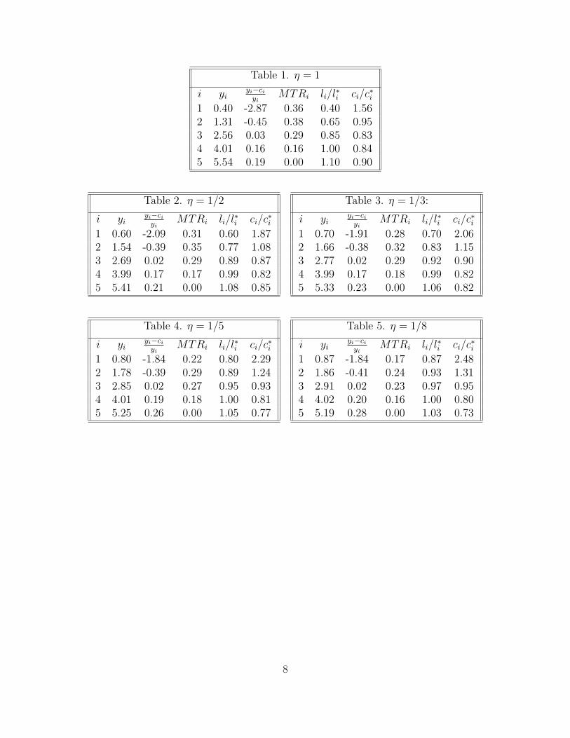
where different values of η correspond to different examples. The zero tax solution is l∗i = 1and c∗i = wi. We compute the solutions for η = 1, 1/2, 1/3, 1/5, 1/8, and report in Tables1-5 the following:

yi, i = 1, .., N,yi − ci

yi

, i = 1, .., N, (average tax rate)

1− ul

wuc

, i = 1, .., N, (marginal tax rate)

li/l∗i , i = 1, .., N,

ci/c∗i , i = 1, .., N,

The pattern of the binding incentive-compatibility constraints is the simple monotonic chainto the left property as expected in nonlinear optimal tax problems in one dimension; seeWeymark (1986). Note that the results are as expected. Marginal and average tax rates onthe types that pay taxes are moderately high, and increase as the elasticity of labor supplyfalls. The subsidy rates to the poor fall as we move from the high-elasticity world to thelow-elasticity world because the high marginal rates the poor face depress their labor supplymuch more in the high-elasticity world; remember, all people in each of these economies havethe same elasticity.

7

Table 1. η = 1

i yiyi−ci

yiMTRi li/l

∗i ci/c

∗i

1 0.40 -2.87 0.36 0.40 1.562 1.31 -0.45 0.38 0.65 0.953 2.56 0.03 0.29 0.85 0.834 4.01 0.16 0.16 1.00 0.845 5.54 0.19 0.00 1.10 0.90

Table 2. η = 1/2

i yiyi−ci

yiMTRi li/l

∗i ci/c

∗i

1 0.60 -2.09 0.31 0.60 1.872 1.54 -0.39 0.35 0.77 1.083 2.69 0.02 0.29 0.89 0.874 3.99 0.17 0.17 0.99 0.825 5.41 0.21 0.00 1.08 0.85

Table 3. η = 1/3:

i yiyi−ci

yiMTRi li/l

∗i ci/c

∗i

1 0.70 -1.91 0.28 0.70 2.062 1.66 -0.38 0.32 0.83 1.153 2.77 0.02 0.29 0.92 0.904 3.99 0.17 0.18 0.99 0.825 5.33 0.23 0.00 1.06 0.82

Table 4. η = 1/5

i yiyi−ci

yiMTRi li/l

∗i ci/c

∗i

1 0.80 -1.84 0.22 0.80 2.292 1.78 -0.39 0.29 0.89 1.243 2.85 0.02 0.27 0.95 0.934 4.01 0.19 0.18 1.00 0.815 5.25 0.26 0.00 1.05 0.77

Table 5. η = 1/8

i yiyi−ci

yiMTRi li/l

∗i ci/c

∗i

1 0.87 -1.84 0.17 0.87 2.482 1.86 -0.41 0.24 0.93 1.313 2.91 0.02 0.23 0.97 0.954 4.02 0.20 0.16 1.00 0.805 5.19 0.28 0.00 1.03 0.73

8

2.2 Multidimensional Heterogeneity

We next consider models with multidimensional heterogeneity. One kind of multidimensionalheterogeneity will be where people differ in both productivity and elasticity of labor supply,η. We will examine that and other types of heterogeneity. More generally, we consider utilityfunctions of the following form

u(c, l) =(c− α)1−1/γ

1− 1/γ− ψ

l1/η+1

1/η + 1, (8)

where α, γ, ψ, and η are possible taxpayer heterogeneities, in addition to wage w. Eachterm has a natural economic interpretation. The parameter α represents basic “needs”, aminimal level of consumption. A high α implies a higher marginal utility of consumptionat any c. The parameter γ represents the elasticity of demand for consumption, whereasthe parameter ψ represents the level of distaste for work. The parameter η represents laborsupply responsiveness to the wage. This general specification implies a five-dimensionalspecification of taxpayer types.

For simplicity, we assume there are N types in each heterogeneities. We also define aproduct index sets T := {1, . . . , N}5. Since wage heterogeneity will always be assumed, let t1always represent the wage type. For each t = (t1, . . . , t5) ∈ T , we denote the utility functionfor type t as6 ut (c, l). The optimal nonlinear income taxation with the utility function (8)is formulated as follows:

max(yt,ct)t∈T∑

t∈T λt ut(ct, yt/wt1)

s.t. u t(ct, yt/wt1)− u t(ct′ , yt′/wt1) ≥ 0 ∀t, t′ ∈ T∑

t∈T ct ≤∑

t∈T yt

∑t∈T ct ≥ 0,

(9)

The problem size is 2|T | variables with |T | ∗ (|T | − 1) nonlinear constraints. Notice thatthe number of constraints is the square of the number of the number of variables. This is afeature of all incentive problems; only in some with simplifying principals like single-crossingare we able to significantly reduce the number of constraints.

2.3 Computational Difficulties with NLPs from Incentive Prob-lems

The nonlinear program (9) is a difficult problem to solve numerically. The objective isconcave, but there is a large number of constraints. Furthermore, there is no reason to

6To minimize notational complexity, we allow the wage type to show up in the notation ut even thoughthe wage type is not an argument of u.

9

believe that the constraints are concave. This creates two problems. First, we cannot ignorethe possibility of multiple local optima. We will deal with this in well-known standard ways,and so will not discuss the details of that

The second problem is more challenging: the failure of useful constraint qualifications.Recall the structure of constrained optimization problems. Consider the inequality con-strained problem

min f(x) subject to c(x) ≥ 0,

where f : Rn → R and c : Rn → Rm are assumed smooth. There are many numericalalgorithms for solving such problems, but they generally assume that the solution, x∗, satisfiessome constraint qualification. Define the set of binding constraints

A∗ = {i = 1, 2, ..., m|ci(x∗) = 0}.

The linear independence constraint qualification (LICQ) states that the gradients, of thebinding constraints, ∇ci(x

∗), i ∈ A, are linearly independent. The Mangasarian-Fromovitzconstraint qualification (MFCQ) assumes that there is a direction such that ∇ci(x

∗)T d > 0for all i ∈ A∗.

In one-dimensional models with single-crossing problems, the LICQ will generally hold.However, multidimensional problems can easily run afoul of the LICQ for one simple reason:if the number of binding constraints exceed the number of constraints, such as in the caseof multidimensional pooling, it is impossible for LICQ to hold. Since multidimensionalproblems are not likely to satisfy a simple pattern of binding incentive constraints. In fact,we found many cases where the LICQ could not hold.

LICQ is a sufficient condition for local convergence of many optimization algorithms,not a necessary condition. However, the failure of LICQ will at least slow down convergence.Our computations converged, but in many cases the number of major iterations needed wasunusually large, sometimes in the order of thousands, even for a two-dimensional problemwith 25 total types. The failure of the LICQ is probably the sole source of difficulties insolving these nonlinear programs. Other issues, such as scaling, e.g., the range of inputparameters w or η, can also cause problems. However, we found LICQ will often fail atsolutions of these problems.

Nonlinear programs with constraint qualification failures have been the object of muchresearch in numerical optimization in the past decade. More generally, much progress hasbeen made on a new class of problems called mathematical programs with equilibrium con-straints (MPECs) [?, ?, ?]. One well-known property about MPECs is that the standardCQs fail at every feasible point. We are optimistic that we will be able to apply thosemethods to allow us to solve larger and more complex problems.

10

3 Numerical Examples

We now examine economies with multiple dimensions of heterogeneity.

3.1 Wage-Labor Supply Elasticity Heterogeneity

We first consider the case where taxpayers differ in terms of their wage, w, and elasticity oflabor supply, η. We assume that α = 0, γ = 1 (log utility), and ψ = 1. We consider anoptimal nonlinear income tax problem with two-dimensional types of taxpayers:

max(yij ,cij)i,j

∑Ni=1

∑Nj=1 λij u j(cij, yij/wi)

s.t. u j(cij, yij/wi)− u j(ci′j′ , yi′j′/wi) ≥ 0, for all (i, j), (i′, j′)∑N

i=1

∑Nj=1 cij ≤

∑Ni=1

∑Nj=1 yij

∑Ni=1

∑Nj=1 cij ≥ 0,

(10)

where u j(c, l) = log c − l1/ηj+1/(1/η j + 1), and (cij, yij) is the allocation for the (i, j)-typetaxpayer. The zero tax solution for type (i, j) is (l∗ij, c

∗ij, y

∗ij) = (1, wi, wi). We choose the

following parameters: N = 5, wi ∈ {1, 2, 3, 4, 5}, ηj ∈ {1, 1/2, 1/3, 1/5, 1/8}, and λij = 1.We use the zero tax solution (c∗, y∗) as a starting point for the NLP solver, SNOPT.

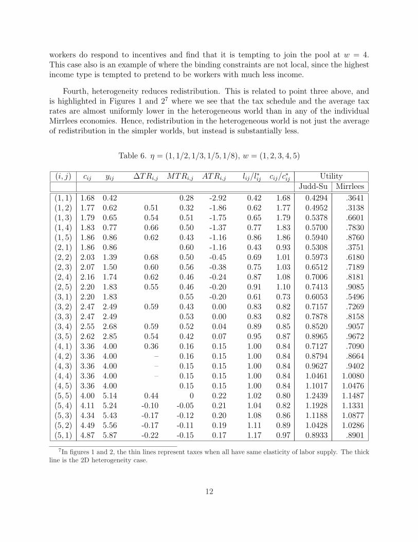
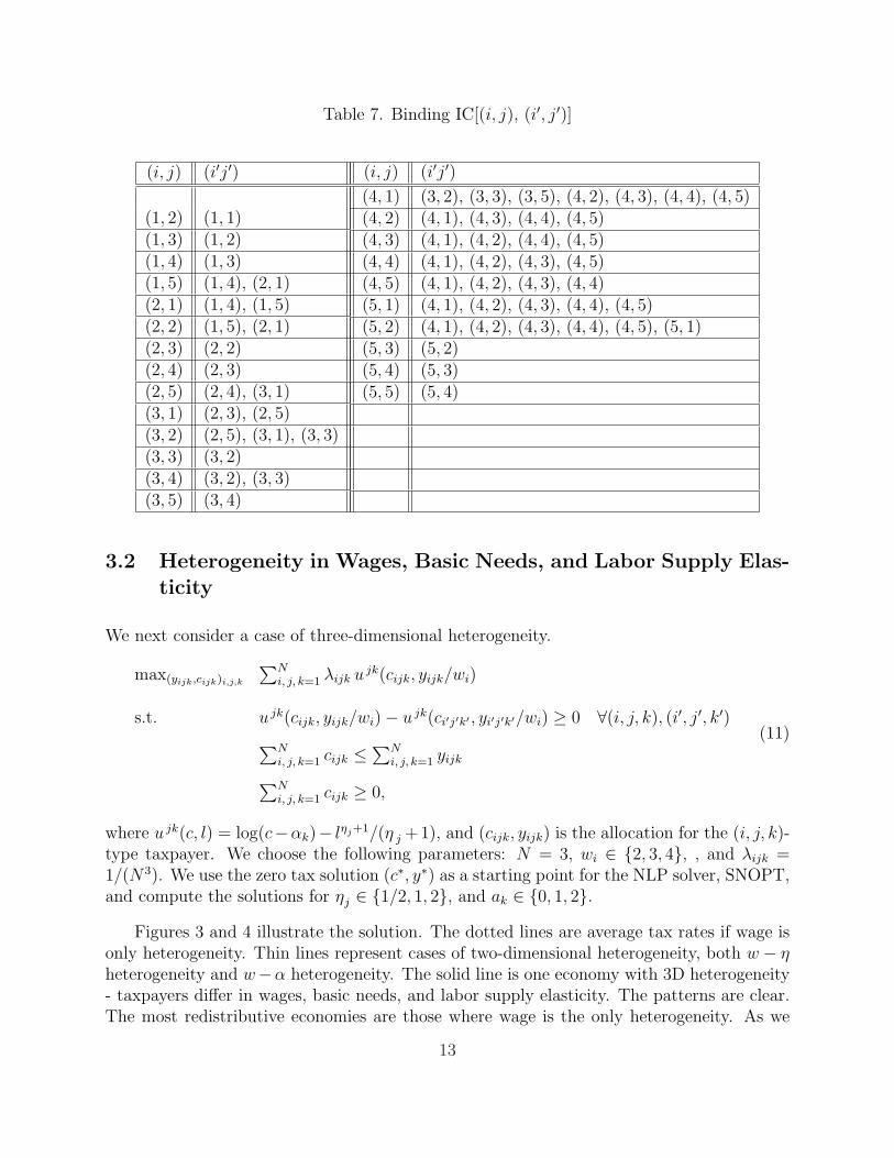
We report numerical results in Tables 6 and 7 below. There are several points to em-phasize.

First, all taxpayers with wage type wi = 4 are pooled. Table 7 shows that there aremany more binding constraints than there are variables. This tells us that our worries aboutfailures of LICQ are well-founded.

Second, this example violates the basic impression that marginal tax rates lie betweenzero and one. Consider taxpayers with wage rate wi = 5. In particular, the taxpayers withlow labor supply elasticity η tend to work less and make less income. However, they paymore tax than those taxpayers with high labor supply elasticity η, who have higher income.We also find negative marginal tax rate for the high productivity types with w = 5. Theseresults are quite different from from the results for one-dimensional type taxpayers, given inTables 1 – 5 as well as general conclusions in optimal income taxation literature.

Third, all high productivity types are better off in the heterogeneous world. We arenot surprised that the low-elasticity high-productivity types are better off since their lowelasticity was exploited in the world where all had low labor supply elasticity. In a heteroge-neous world, the average elasticity of labor is higher, and so there should be lower taxes onhigh-productivity workers. The surprise is that the high-elasticity, high-productivity workersalso gain by hiding in a heterogeneous world. The reason, as seen in Table 7, is that these

11

workers do respond to incentives and find that it is tempting to join the pool at w = 4.This case also is an example of where the binding constraints are not local, since the highestincome type is tempted to pretend to be workers with much less income.

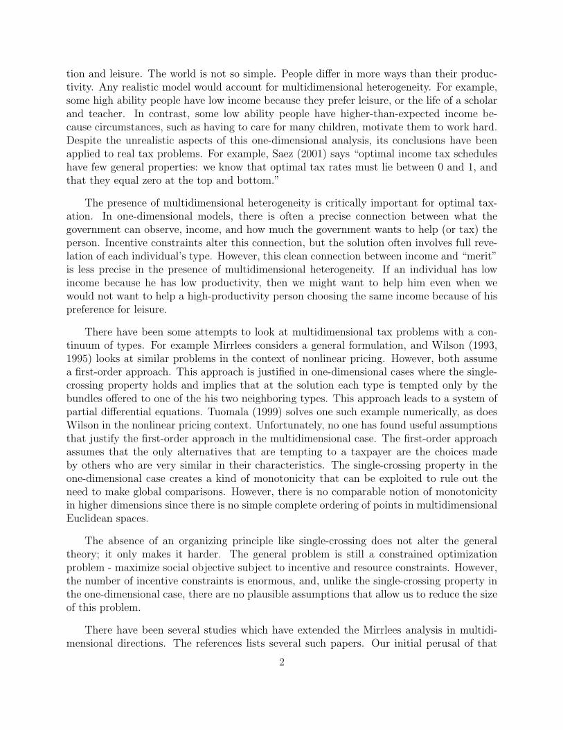
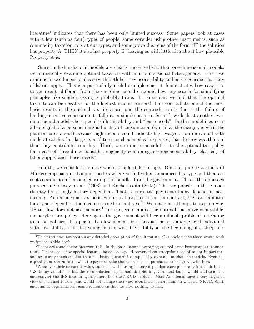
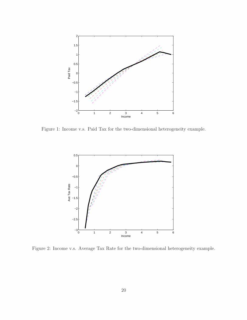
Fourth, heterogeneity reduces redistribution. This is related to point three above, andis highlighted in Figures 1 and 27 where we see that the tax schedule and the average taxrates are almost uniformly lower in the heterogeneous world than in any of the individualMirrlees economies. Hence, redistribution in the heterogeneous world is not just the averageof redistribution in the simpler worlds, but instead is substantially less.

Table 6. η = (1, 1/2, 1/3, 1/5, 1/8), w = (1, 2, 3, 4, 5)

(i, j) cij yij ∆TRi,j MTRi,j ATRi,j lij/l∗ij cij/c

∗ij Utility

Judd-Su Mirrlees

(1, 1) 1.68 0.42 0.28 -2.92 0.42 1.68 0.4294 .3641(1, 2) 1.77 0.62 0.51 0.32 -1.86 0.62 1.77 0.4952 .3138(1, 3) 1.79 0.65 0.54 0.51 -1.75 0.65 1.79 0.5378 .6601(1, 4) 1.83 0.77 0.66 0.50 -1.37 0.77 1.83 0.5700 .7830(1, 5) 1.86 0.86 0.62 0.43 -1.16 0.86 1.86 0.5940 .8760(2, 1) 1.86 0.86 0.60 -1.16 0.43 0.93 0.5308 .3751(2, 2) 2.03 1.39 0.68 0.50 -0.45 0.69 1.01 0.5973 .6180(2, 3) 2.07 1.50 0.60 0.56 -0.38 0.75 1.03 0.6512 .7189(2, 4) 2.16 1.74 0.62 0.46 -0.24 0.87 1.08 0.7006 .8181(2, 5) 2.20 1.83 0.55 0.46 -0.20 0.91 1.10 0.7413 .9085(3, 1) 2.20 1.83 0.55 -0.20 0.61 0.73 0.6053 .5496(3, 2) 2.47 2.49 0.59 0.43 0.00 0.83 0.82 0.7157 .7269(3, 3) 2.47 2.49 0.53 0.00 0.83 0.82 0.7878 .8158(3, 4) 2.55 2.68 0.59 0.52 0.04 0.89 0.85 0.8520 .9057(3, 5) 2.62 2.85 0.54 0.42 0.07 0.95 0.87 0.8965 .9672(4, 1) 3.36 4.00 0.36 0.16 0.15 1.00 0.84 0.7127 .7090(4, 2) 3.36 4.00 – 0.16 0.15 1.00 0.84 0.8794 .8664(4, 3) 3.36 4.00 – 0.15 0.15 1.00 0.84 0.9627 .9402(4, 4) 3.36 4.00 – 0.15 0.15 1.00 0.84 1.0461 1.0080(4, 5) 3.36 4.00 0.15 0.15 1.00 0.84 1.1017 1.0476(5, 5) 4.00 5.14 0.44 0 0.22 1.02 0.80 1.2439 1.1487(5, 4) 4.11 5.24 -0.10 -0.05 0.21 1.04 0.82 1.1928 1.1331(5, 3) 4.34 5.43 -0.17 -0.12 0.20 1.08 0.86 1.1188 1.0877(5, 2) 4.49 5.56 -0.17 -0.11 0.19 1.11 0.89 1.0428 1.0286(5, 1) 4.87 5.87 -0.22 -0.15 0.17 1.17 0.97 0.8933 .8901

7In figures 1 and 2, the thin lines represent taxes when all have same elasticity of labor supply. The thickline is the 2D heterogeneity case.

12

Table 7. Binding IC[(i, j), (i′, j′)]

(i, j) (i′j′)

(1, 2) (1, 1)(1, 3) (1, 2)(1, 4) (1, 3)(1, 5) (1, 4), (2, 1)(2, 1) (1, 4), (1, 5)(2, 2) (1, 5), (2, 1)(2, 3) (2, 2)(2, 4) (2, 3)(2, 5) (2, 4), (3, 1)(3, 1) (2, 3), (2, 5)(3, 2) (2, 5), (3, 1), (3, 3)(3, 3) (3, 2)(3, 4) (3, 2), (3, 3)(3, 5) (3, 4)

(i, j) (i′j′)(4, 1) (3, 2), (3, 3), (3, 5), (4, 2), (4, 3), (4, 4), (4, 5)(4, 2) (4, 1), (4, 3), (4, 4), (4, 5)(4, 3) (4, 1), (4, 2), (4, 4), (4, 5)(4, 4) (4, 1), (4, 2), (4, 3), (4, 5)(4, 5) (4, 1), (4, 2), (4, 3), (4, 4)(5, 1) (4, 1), (4, 2), (4, 3), (4, 4), (4, 5)(5, 2) (4, 1), (4, 2), (4, 3), (4, 4), (4, 5), (5, 1)(5, 3) (5, 2)(5, 4) (5, 3)(5, 5) (5, 4)

3.2 Heterogeneity in Wages, Basic Needs, and Labor Supply Elas-ticity

We next consider a case of three-dimensional heterogeneity.

max(yijk,cijk)i,j,k

∑Ni, j, k=1 λijk u jk(cijk, yijk/wi)

s.t. u jk(cijk, yijk/wi)− u jk(ci′j′k′ , yi′j′k′/wi) ≥ 0 ∀(i, j, k), (i′, j′, k′)∑N

i, j, k=1 cijk ≤∑N

i, j, k=1 yijk

∑Ni, j, k=1 cijk ≥ 0,

(11)

where u jk(c, l) = log(c−αk)− lηj+1/(η j +1), and (cijk, yijk) is the allocation for the (i, j, k)-type taxpayer. We choose the following parameters: N = 3, wi ∈ {2, 3, 4}, , and λijk =1/(N3). We use the zero tax solution (c∗, y∗) as a starting point for the NLP solver, SNOPT,and compute the solutions for ηj ∈ {1/2, 1, 2}, and ak ∈ {0, 1, 2}.

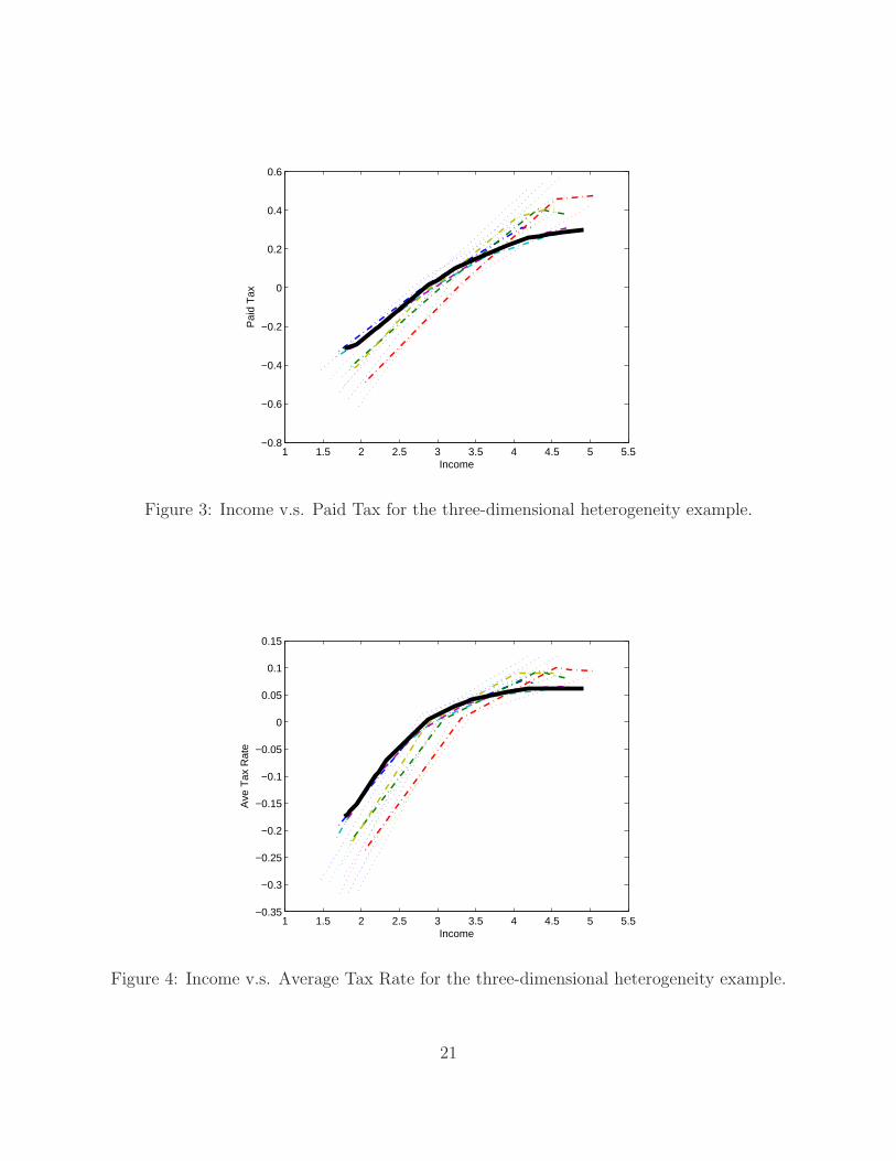
Figures 3 and 4 illustrate the solution. The dotted lines are average tax rates if wage isonly heterogeneity. Thin lines represent cases of two-dimensional heterogeneity, both w − ηheterogeneity and w−α heterogeneity. The solid line is one economy with 3D heterogeneity- taxpayers differ in wages, basic needs, and labor supply elasticity. The patterns are clear.The most redistributive economies are those where wage is the only heterogeneity. As we

13

add heterogeneity in either α or η, redistribution is less. The final case where there isheterogeneity in wages, basic needs, and elasticity, has the least redistribution.

3.3 Wage-Age Heterogeneity

Our final example is a case where people differ by productivity and age. If we apply theMirrlees approach to dynamic models, the result will be age-dependent income-consumptionallocations. This is not the case for actual tax systems. Instead, tax liabilities generallydepend only on the current year’s income. We will examine the optimal tax policy underthe assumption that tax liabilities depend only on current income. Implicit in this are manylimitations on the government policy. In particular, we will not allow the government to usecurrent consumption nor current assets in determining taxes.

The way to do this is to impose more constraints on the income-consumption bundles. Inour example, we will assume that there are four types of workers who live for three periods.From the point of view of a government that cannot see age, there are twelve types of peopleand the optimal tax policy will offer twelve consumption-income bundles. Each individualwill choose a life-cycle pattern from that menu. There are 1728 possible paths to choosefrom. The incentive compatibility constraint will say that each individual will freely choosethat one life-cycle path that the government has prescribed for him. Since there are threetypes of people, there are 6912 incentive constraints.

We assume that there are four types of workers, and that each type has deterministicpattern of life-cycle wages. We use the following numerical specification:

Wage HistoryPeriod

Type t1 t2 t31 1 3 22 2 4 43 2 5 44 3 5 6

Kocherlakota, and Golosov et al. have applied the Mirrlees approach to this model, whereeach individual announces his type when born, and then is given a life-cycle pattern of incomeand taxes that he must follow. We argued above that this kind of history dependence doesnot describe existing tax policies. Therefore, we look at three cases: Mirrlees taxation, anoptimal (nonlinear) tax on workers that are consistent with the ability of each worker to,and the optimal linear tax policy.

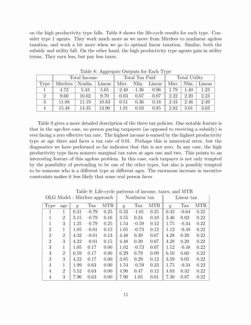
We first see that as we add more restrictions, going from Mirrlees to optimal age-independent policy to linear tax, the amount of redistribution falls and the tax burden

14

on the high productivity type falls. Table 8 shows the life-cycle results for each type. Con-sider type 1 agents. They work much more as we move from Mirrlees to nonlinear agelesstaxation, and work a bit more when we go to optimal linear taxation. Similar, both thesubsidy and utility fall. On the other hand, the high productivity type agents gain in utilityterms. They earn less, but pay less taxes.

Table 8: Aggregate Outputs for Each TypeTotal Income Total Tax Paid Total Utility

Type Mirrlees Nonlin. Linear Mirr. Nlin. Linear Mirr. Nlin. Linear1 4.72 5.43 5.65 –2.40 –1.36 –0.96 1.79 1.40 1.232 9.60 10.02 9.70 –0.03 0.07 –0.07 2.22 2.20 2.233 11.88 11.19 10.83 0.51 0.36 0.18 2.43 2.46 2.494 15.48 14.35 13.90 1.91 0.93 0.85 2.82 3.01 3.03

Table 9 gives a more detailed description of the three tax policies. One notable feature isthat in the age-free case, no person paying taxpayers (as opposed to receiving a subsidy) isever facing a zero effective tax rate. The highest income is earned by the highest productivitytype at age three and faces a tax rate of 0.01. Perhaps this is numerical error, but thediagnostics we have performed so far indicates that this is not zero. In any case, the highproductivity type faces nonzero marginal tax rates at ages one and two. This points to aninteresting feature of this ageless problem. In this case, each taxpayer is not only temptedby the possibility of pretending to be one of the other types, but also is possibly temptedto be someone who is a different type at different ages. The enormous increase in incentiveconstraints makes it less likely that some real person faces

Table 9: Life-cycle patterns of income, taxes, and MTROLG Model - Mirrlees approach

Type age y Tax MTR1 1 0.31 –0.79 0.251 2 3.15 –0.79 0.161 3 1.25 –0.79 0.252 1 1.05 –0.01 0.152 2 4.32 –0.01 0.132 3 4.22 –0.01 0.153 1 1.05 0.17 0.003 2 6.59 0.17 0.003 3 4.22 0.17 0.004 1 1.99 0.63 0.004 2 5.52 0.63 0.004 3 7.96 0.63 0.00

Nonlinear tax

y Tax MTR0.32 –1.01 0.253.55 0.24 0.101.54 –0.59 0.121.05 –0.73 0.124.48 0.39 0.074.48 0.39 0.071.02 –0.73 0.076.29 0.79 0.093.85 0.29 0.121.54 –0.59 0.234.90 0.47 0.127.90 1.05 0.01

Linear tax

y Tax MTR0.42 –0.64 0.223.46 0.02 0.221.75 –0.34 0.221.12 –0.48 0.224.28 0.20 0.224.28 0.20 0.221.12 –0.48 0.226.10 0.60 0.223.59 0.05 0.221.75 –0.34 0.224.83 0.32 0.227.30 0.87 0.22

15

4 Conclusions

We have examined some simple cases of optimal taxation in economies with multiple di-mensions of heterogeneities. These examples show that many results from the basic one-dimensional Mirrlees model no longer hold. The examples also indicate that redistributionis much less in economies with multidimensional heterogeneity, probably because income isa noisier signal of a taxpayer’s type. This last result is very provisional until we do a robustexamination of this issue across alternative parameter values for tastes.

The other main point is that these problems are difficult to solve numerically, but theycan be solved if one recognizes the critical numerical difficulties and uses the appropriatesoftware.

16

5 References

Atkinson, A.B. and J.E. Stiglitz (1976), The Design of Tax Structure: Direct versus IndirectTaxation, Journal of Public Economics 6, 55-75.

Blomquist, S., Christiansen, V. (2004). Taxation and Heterogeneous Preferences. Upp-sala Universitet Working Paper 9, Department of Economics.

Blomquist, S. and L. Micheletto (2003). Age Related Optimal Income Taxation, WorkingPaper 2003:7, Department of Economics, Uppsala University.

Boadway R.; Marchand M.; Pestieau P., del Mar Racionero M. (2002): Optimal Redis-tribution with Heterogeneous Preferences for Leisure, Journal of Public Economic Theory 4(no. 4), 475-498.

Boadway, R., Cuff, K., Marchand, M., 2000. Optimal income taxation with quasi-linearpreferences revisited. Journal of Public Economic Theory 2, 435– 460.

Brito, D.L., Oakland, W., 1977. Some properties of the optimal income-tax. Interna-tional Economic Review 18, 407–423.

Cuff, K. (2000). Optimality of Workfare with Heterogeneous Preferences. CanadianJournal of Economics 33, 149-174.

Diamond, P.A., 1998. Optimal income taxation: A example with a U-shaped pattern ofoptimal marginal tax rates. American Economic Review 88, 83– 95.

Ebert, U., 1992. A reexamination of the optimal nonlinear income tax. Journal of PublicEconomics 49, 47– 73.

Ebert, U. (1988). Optimal Income Taxation: On theCase of Two-Dimensional Popula-tions. Discussion Paper A169.

Golosov, Mikhail, Narayana Kocherlakota, and Aleh Tsyvinski, 2003. “Optimal Indirectand Capital Taxation.” Review of Economic Studies. 70 (3): 569–587.

Guesnerie, R., and J. Seade. (1982). Nonlinear pricing in a finite economy. Journal ofPublic Economics 17, 157-179.

Kocherlakota, Narayana R., 2005. “Zero Expected Wealth Taxes: A Mirrlees Approachto Dynamic Optimal Taxation.” Econometrica. 73 (5): 1587–1621.

Laffont, J.-J., Maskin, E., Rochet, J.-C., 1987. Optimal nonlinear pricing with two-dimensional characteristics. In: Groves, T., Radner, R., Reiter, S. (Eds.), Information,Incentives, and Economic Mechanisms. University of Minnesota Press, Minneapolis, pp.256–266.

17

Marchand, M., Pestieau, P. (2003). Optimal redistribution when workers are indistin-guishable. Canadian Journal of Economics, 36, 911–922.

McAfee, R.P., McMillan, J., 1988. Multidimensional incentive compatibility and mech-anism design. Journal of Economic Theory 46, 335–354.

Mirrlees, J.A., 1971. An exploration in the theory of optimum income taxation. Reviewof Economic Studies 38, 175–208.

Mirrlees, J.A., 1976. Optimum tax theory: A synthesis. Journal of Public Economics 7,327–358.

Mirrlees, J.A., 1997. Optimal marginal taxes at low incomes. Unpublished manuscript,Faculty of Economics, University of Cambridge.

Mirrlees, J.A. (1986). The theory of optimal taxation. In Arrow, K.J. and Intriligator,M.D. (eds.), Handbook of Mathematical Economics. Vol. III, Elsevier Science Publishers,B.V., Amsterdam.

Rochet, J.-C., Stole, L.A., 2000. The economics of multidimensional screening. In: De-watripont, M., Hansen, L., Turnovsky, S. (Eds.), Advances in Economics and Econometrics:Eighth World Congress. Cambridge University Press, Cambridge.

Sandmo, A. (1993) : Optimal Redistribution when Tastes Differ, Finanz Archiv 50(2),149-163.

Sandmo, A., 1998. Redistribution and the marginal cost of public funds. Journal ofPublic Economics 70, 365–382.

Seade, J.K., 1977. On the shape of optimal tax schedules. Journal of Public Economics7, 203–235.

Shapiro, J., 1999. Income maintenance programs and multidimensional screening. Un-published manuscript, Department of Economics, Princeton University.

Sheshinski, E., 1971. On the theory of optimal income taxation. Discussion Paper No.172, Harvard Institute for Economic Research, Harvard University.

Stiglitz, J.E. (1982). Self-Selection and Pareto Efficient Taxation. Journal of PublicEconomics 17, 213-240.

Tarkianen, R. and M. Tuomala (1999). Optimal Nonlinear Income Taxation with aTwo-Dimensional Population; A Computational Approach. Computational Economics 13,1-16.

Tuomala, M. (1990). Optimal Income Tax and Redistribution. Clarendon Press, Oxford,U.K.

18

Tuomala, M. (1984). On the optimal income taxation: Some further numerical results.Journal of Public Economics, 23, 351–366.

Weymark, J. A. (1986). A reduced-form of optimal nonlinear income tax problem. Jour-nal of Public Economics, 30, 199–217.

Wilson, R. (1993). Nonlinear Pricing. Oxford University Press, New York.

Wilson, R. (1995). Nonlinear pricing and mechanism design. In Amman, H., Kendrick,D. and Rust, J. (eds.), Handbook of Computational Economics. Vol. 1, Elsevier SciencePublishers B.V., Amsterdam.

19

0 1 2 3 4 5 6−2

−1.5

−1

−0.5

0

0.5

1

1.5

2

Income

Pai

d T

ax

Figure 1: Income v.s. Paid Tax for the two-dimensional heterogeneity example.

0 1 2 3 4 5 6−3

−2.5

−2

−1.5

−1

−0.5

0

0.5

Income

Ave

Tax

Rat

e

Figure 2: Income v.s. Average Tax Rate for the two-dimensional heterogeneity example.

20

1 1.5 2 2.5 3 3.5 4 4.5 5 5.5−0.8

−0.6

−0.4

−0.2

0

0.2

0.4

0.6

Income

Pai

d T

ax

Figure 3: Income v.s. Paid Tax for the three-dimensional heterogeneity example.

1 1.5 2 2.5 3 3.5 4 4.5 5 5.5−0.35

−0.3

−0.25

−0.2

−0.15

−0.1

−0.05

0

0.05

0.1

0.15

Income

Ave

Tax

Rat

e

Figure 4: Income v.s. Average Tax Rate for the three-dimensional heterogeneity example.

21