UNIVERSITÉ DE GENÈVE FACULTÉ DES S CIENCES DÉPARTEMENT DE PHYSIQUE APPLIQUÉE Professeur Nicolas Brunner DÉPARTEMENT DE PHYSIQUE APPLIQUÉE I NSTITUE FOR QUANTUM OPTICS AND QUANTUM I NFORMATION VIENNA (IQOQI VIENNA) Docteur Marcus Huber Optimal Manipulation Of Correlations And Temperature In Quantum Thermodynamics THÈSE Présentée à la Faculté des sciences de l’Université de Genève Pour obtenir le grade de Docteur ès sciences, mention Physique Par Fabien C LIVAZ de Chermignon (VS) Thèse N°5476 GENÈVE Atelier Repromail, Université de Genève 2020 arXiv:2012.04321v1 [quant-ph] 8 Dec 2020
Transcript
UNIVERSITÉ DE GENÈVE FACULTÉ DES SCIENCES
DÉPARTEMENT DE PHYSIQUE APPLIQUÉE Professeur Nicolas BrunnerDÉPARTEMENT DE PHYSIQUE APPLIQUÉE
INSTITUE FOR QUANTUM OPTICS AND QUANTUM
INFORMATION VIENNA (IQOQI VIENNA) Docteur Marcus Huber
Optimal Manipulation Of CorrelationsAnd Temperature In Quantum
Thermodynamics
THÈSEPrésentée à la Faculté des sciences de l’Université de Genève
Pour obtenir le grade de Docteur ès sciences, mention Physique
Par
Fabien CLIVAZde
Chermignon (VS)
Thèse N°5476
GENÈVEAtelier Repromail, Université de Genève
2020
arX
iv:2
012.
0432
1v1
[qu
ant-
ph]
8 D
ec 2
020
i
UNIVERSITY OF GENEVA
AbstractSciences
Department of Applied Physics
Doctor of Physics
Optimal Manipulation Of Correlations And Temperature In QuantumThermodynamics
by Fabien CLIVAZ
This thesis is devoted to the study of two tasks: refrigeration and the creationof correlations. Both of these tasks are investigated within the realm of quantumthermodynamics. Our approach is influenced by that of quantum information butconnections with other approaches are desired and emphasized whenever possible.
Cooling is one of the tasks of paramount importance of quantum thermodynamicsand thermodynamics itself. Reaching cold temperatures is of undisputed techno-logical relevance and ubiquitous among the many sub-fields of physics, allowing,on the one hand, to reach fascinating states of matter such as superconductivityor Bose-Einstein condensation, while, on the other hand, being a fundamentallyimposed background constraint in areas such as astrophysics. In thermodynamics,temperature plays a special role in that it is one of the premises of the theory. Whileits value is unbounded from above, its statistical physical interpretation sets a hardlower bound that is by now thought of as inherent to the theory. Investigating howthis lower bound can be attained within the framework of quantum theory is thusintimately related to the understanding of the fundamental laws that dictate quantumthermodynamics. It is therefore of no surprise that many different cooling schemesemerged from different approaches of quantum thermodynamics in the recent lit-erature on the subject. While each of these approaches work with their own set ofassumptions, they all have in common that
1. they assume a background temperature and with it an available thermal state,
2. the system to be cooled is in some sort open/connected to the environment.
The first assumption is actually not obvious at all and understanding how andunder which circumstances one can assume a given closed system to be thermal ison its own an exciting and active research field. However, once the existence of athermal state is accepted, in order for anything to happen to the state, 2. has to hold.The diversity of the approaches is then formed in how exactly the system is open toits environment. Our take on it consists in dividing the environment in two parts:a “machine” and the rest of the environment. While the rest of the environment isthought of as being weakly or not controlled in that it is only used to rethermalizethe machine, we assume an increased control on the part of the environment we call“machine”, hence the name. To prevent any hidden energy supply, we furthermoreexplicitly take the source of energy into account. This gives rise to two variations ofour paradigm. In the incoherent version the machine benefits from a fully entropicsource of energy and is controlled in an energy conserving manner. In the coherentone, the source of energy is provided in an entropy-less manner and we allow forfull unitary control. Both variations of this paradigm are designed to be related toother existing approaches and as such provide a common platform to on the onehand unify these approaches and on the other hand compare their performances onan equal footing.
Investigating each of our paradigms we furthermore find a bound that holdsfor both of our paradigms and that is attainable under minimal assumptions for allfinite dimensional systems and machines. The bound is in particular a single letterbound that does not depend on the particular intricacies of the system and machine,and as such identifies the relevant parameter of interest, fulfilling one of the centralgoal of statistical physics. The bound is furthermore already attainable for minimalmachines. Investigating these minimal machines in greater details, we find that theenergy spent for achieving this bound is dependent on the level of control and thatfor non-maximal cooling there is no universally better paradigm that achieves a giventemperature in terms of energy expenditure.
Our second task of interest, the creation of correlations, is motivated by a fun-damental property of our current understanding of nature: correlations lie at theheart of every scientific prediction. It is therefore natural to wonder how much corre-lations can be created at a finite amount of invested energy. Assuming an initiallyuncorrelated system in a thermal background, it can be shown that the creation ofcorrelations comes at an energy cost. In other words, no correlation is for free in thatcontext. Viewing correlations as the resource of information theory and energy asthat of thermodynamics, the above stipulates that the acquisition of information ina physical system necessarily comes at a thermodynamic cost. While lower boundson the amount of energy that has to be invested in the process can be formulated,their reachability remains an open question. We here derive a framework that allowsto investigate this question more closely for a pair of initially uncorrelated identicalsystems in a thermal background. This framework is based on decomposing theHilbert space in a Latin square manner and as such allows us to harness the toolsof majorization theory. Doing so, we are able to provide protocols that achieve thelower bound for any 3 dimensional and 4 dimensional systems. We furthermoreprovide a set of conditions to be fulfilled in order for the bound to be achievable inany dimension.
iii
Résumé
Cette thèse est consacrée à l’étude de deux tâches: la réfrigération et la création decorrélations. Ces deux tâches sont étudiées du point de vue de la thermodynamiquequantique. Notre approche est influencée par celle de l’information quantique, maisdes connexions avec d’autres approches sont souhaitées et soulignées dans la mesuredu possible.
Le refroidissement est l’une des tâches de la plus haute importance de la thermo-dynamique quantique et de la thermodynamique elle-même. Atteindre des tempéra-tures froides est d’une pertinence technologique incontestée et omniprésente parmiles nombreux sous-domaines de la physique, nous permettant d’une part d’atteindredes états fascinants de la matière tels que la supraconductivité ou la condensationde Bose-Einstein, tout en étant d’autre part tout simplement une contrainte de fondimposée fondamentalement dans des domaines tels que l’astrophysique. En ther-modynamique, la température joue un rôle particulier en ce qu’elle est l’une desprémisses de la théorie. Bien que sa valeur ne soit pas bornée en haut, son inter-prétation physique statistique établit une borne inférieure dure qui est désormaisconsidérée comme inhérente à la théorie. Étudier comment cette limite inférieurepeut être atteinte dans le cadre de la théorie quantique est donc intimement lié à lacompréhension des lois fondamentales qui dictent la thermodynamique quantique.Il n’est donc pas surprenant que de nombreux schémas de refroidissement différentsaient émergé de différentes approches de la thermodynamique quantique dans lalittérature récente sur le sujet. Bien que chacune de ces approches fonctionne avecson propre ensemble d’hypothèses, elles ont toutes en commun que
1. elles supposent une température de fond et avec elle un état thermique disponible,
2. le système à refroidir est d’une manière ou d’une autre ouvert sur l’environnement.
La première hypothèse n’est en fait pas évidente du tout et comprendre commentet dans quelles circonstances on peut supposer qu’un système donné en contact avecun environnement soit thermique est en soi un domaine de recherche passionnantet actif. Cependant, une fois que l’existence d’un état thermique est acceptée, pourque quelque chose arrive à l’état, 2. est forcé d’être vrai. La diversité des approchesse forme alors dans la façon dont le système est ouvert à son environnement. Notreapproche consiste à diviser l’environnement en deux parties: une “machine” et lereste de l’environnement. Alors que le reste de l’environnement est considéré commefaiblement ou non contrôlé en ce qu’il n’est utilisé que pour rethermaliser la ma-chine, nous supposons un contrôle accru de la part de l’environnement que nousappelons “machine”, d’où le nom. Pour éviter tout approvisionnement énergétiquecaché, nous tenons en outre explicitement compte de la source d’énergie. Cela donnelieu à deux variantes de notre paradigme. Dans la version incohérente, la machinebénéficie d’une source d’énergie entièrement entropique et est contrôlée d’une façonconservant l’énergie. Dans la version cohérente, la source d’énergie est fournie sansentropie et nous permettons un contrôle unitaire complet. Les deux variantes de ce
iv
paradigme sont conçues pour être liées à d’autres approches existantes et, en tant quetelles, fournissent une plate-forme commune qui d’un côté unifie ces approches et,d’autre part, compare leurs performances sur un même pied d’égalité.
En étudiant chacun de nos paradigmes en tant que tel, nous trouvons en outre uneborne qui s’applique à nos deux paradigmes et qui est réalisable sous des hypothèsesminimales pour tous les systèmes et machines de dimension finie. La borne est enparticulier de type lettre unique et ne dépend pas des subtilités particulières dusystème et de la machine, et en tant que telle identifie le paramètre d’intérêt pertinent,remplissant l’un des piliers centraux de la physique statistique. La borne est en outredéjà atteignable pour des machines minimales. En étudiant ces machines minimalesde façon plus détaillée, nous constatons que l’énergie dépensée pour atteindre cetteborne dépend du niveau de contrôle et que pour un refroidissement non maximal, iln’y a pas de paradigme universellement meilleur qui atteint une température donnéeen termes de dépense énergétique.
Notre deuxième tâche d’intérêt, la création de corrélations, est motivée par unepropriété fondamentale de notre compréhension actuelle de la nature: les corrélationssont au cœur de toute prédiction scientifique. Il est donc naturel de se demandercombien de corrélations peuvent être créées pour une quantité finie d’énergie investie.En supposant un système initialement non corrélé dans un contexte thermique,il peut être démontré que la création de corrélations a un coût énergétique. End’autres termes, aucune corrélation n’est gratuite dans ce contexte. Considérant lescorrélations comme la ressource de la théorie de l’information et l’énergie commecelle de la thermodynamique, ce qui précède stipule que l’acquisition d’informationsdans un système physique a nécessairement un coût thermodynamique. Alors quedes bornes inférieures sur la quantité d’énergie qui doit être investie dans le processuspeuvent être formulées, leur atteignabilité reste une question ouverte. Nous dérivonsici un cadre qui permet d’étudier cette question de plus près pour une paire desystèmes identiques initialement non corrélés dans un contexte thermique. Ce cadreest basé sur la décomposition de l’espace de Hilbert de type carré latin et à ce titrenous permet d’exploiter les outils de la théorie de la majorisation. Ce faisant, noussommes en mesure de fournir des protocoles qui atteignent la borne inférieure pourtous les systèmes de dimension 3 et 4. Nous fournissons en outre un ensemblede conditions à remplir pour que la borne soit atteignable dans n’importe quelledimension.
v
AcknowledgementsI would like to first of all thank both of my supervisors, Nicolas Brunner and
Marcus Huber, for their invaluable support throughout my PhD. In particular, thankyou to both of them for having given me the freedom and flexibility I needed whileat the same time providing guidance, clarity, a whole lot of precious ideas, as well asa fruitful research context.
On the Geneva side, my gratitude extends to the whole quantum theory groupas well as the GAP. Thank you in particular to Ralph Silva for the tight and fruitfulcollaboration that developed throughout the years. I equally thank Géraldine Haackand Jonatan Bohr Brask in that regard. Thank you also to Flavien Hirsch who has bynow become a precious research companion.
On the Vienna side, I am grateful to the entire Huber group. Thank you to NicolaiFriis for his helpful scientific support. Thank you also to Faraj Bakhshinezhad forhis incredible perseverance. And thank you to Jessica Bavaresco for her wise andbeneficial advice.
I would also like to thank Philip Taranto, Falvien Hirsch, Raya Polishchuk, Mar-cus Huber, Nicolas Brunner, Géraldine Haack, Martí Perarnau-Llobet, and AndreasWinter for valuable feedback on and around this manuscript.
Thank you also to Kristina Eisfeld, Raya Polishchuk, and Tatjana Boczy for creat-ing an online working space that enabled me to keep being productive in writing thisthesis while being confined at home due to the Covid-19 measures.
Last but not least, I would like to wholeheartedly thank my family, friends,colleagues, and others who have contributed in what one may describe as a moreindirect but at least as important way to the academic path I have taken so far. A veryspecial thanks in that regard goes to my wife, Raya, who besides having contributedin the specific above mentioned instances, has been an incredible source of continuouslove and support throughout the years. I feel very privileged to be lucky enough tohave you in my life.
• F. Bakhshinezhad, F. Clivaz, G. Vitagliano, P. Erker, A. Rezakhani, M. Huber,and N. Friis, "Thermodynamically optimal creation of correlations," Journal ofPhysics A: Mathematical and Theoretical 52, 465303 (2019), arXiv:1904.07942.
• F. Clivaz, R. Silva, G. Haack, J. Bohr Brask, N. Brunner, and M. Huber, "Unifyingparadigms of quantum refrigeration: A universal and attainable bound oncooling," Phys. Rev. Lett. 123, 170605 (2019), arXiv:1903.04970.
• F. Clivaz, R. Silva, G. Haack, J. Bohr Brask, N. Brunner, and M. Huber, "Uni-fying paradigms of quantum refrigeration: fundamental limits of cooling andassociated work costs," Phys. Rev. E 100, 042130 (2019), arXiv:1710.11624.
It is a delicate task to define a research field, especially when it is still very muchactive. On the one hand, one would like to include all what is done in the directionthat the supposed field investigates. On the other hand, delimiting it in too broadterms might inadvertently include research that definitely considers itself as beingoutside of the said field. That being said, the research that formed the basis of thisthesis can be classified as being part of the field of quantum thermodynamics. Quan-tum thermodynamics is a hybrid field that studies the interplay between two majortheories of physics: quantum mechanics and thermodynamics. The motivations fordoing so are quite diverse. From a theoretical perspective both theories are strikinglycomplementary. Quantum mechanics is the widely accepted theory of microscopic ob-jects, while thermodynamics is very effective at describing macroscopic phenomena.It is therefore appealing to:
1. Investigate how the thermodynamic behavior of macroscopic systems emergesfrom their microscopic quantum mechanical description.
2. Extend useful thermodynamic concepts such as temperature, heat, work andentropy to the quantum mechanical realm.
From a practical viewpoint, the recent miniaturization of technologies naturallypushes for the development of a theory that allows to best engineer them. This istimely, as it is complemented with our increased ability to control larger and largerquantum systems, giving us the opportunity to experimentally test theoretical ideas.
The dialogue between thermodynamics and quantum mechanics started rightat the dawn of quantum mechanics: in 1905 Einstein introduced the concept of aphoton by, using a thermodynamic argument, studying the photoelectric effect [1].Despite this intimate relation, quantum mechanics and thermodynamics branchedoff in the following decades to further develop independently of each other. Onlyin 1959, when the first solid state lasers were developed, did the two fields meetagain as Scovil and Schulz DuBois [2] discovered the equivalence between the threelevel maser and the Carnot heat engine [3]. The former was developed thanks toour understanding of stimulated emission, a truly quantum mechanical phenomena,while the latter is a pillar of thermodynamics. Their seminal work set the stage for therich field of quantum thermodynamics that would blossom in the decades to come.
Due to its broad scope, the field has attracted researchers from many backgrounds,ranging from statistical physics, many-body theory, and quantum optics to meso-scopic physics and quantum information theory [4]. This diversity is reflected both inthe number of different sub fields and the different approaches found to address agiven question, where consensus is sometimes yet to be reached [5].
Chapter 1. Research Context 3
One of the most fundamental questions that has been asked since the beginningof thermodynamics and statistical physics regards the problem of equilibration andthermalization [4, 6]: why do systems tend to equilibrate? Early contributions to thetopic date back to the works of Schrödinger in 1927 [7] and von Neumann in 1929[8]. See [9] for an English translation of the work of von Neumann. It is, however,only recently that we were able to gain more understanding onto this challengingtopic. Current research in this direction is contributing to the understanding of whymany-body systems appear to equilibrate and the time-scales under which they doso. A large body of work also investigates the properties of many-body systems atthermal equilibrium, such as their correlations. Notions such as (dynamical) typicality[7–12] and the eigenstates thermalization hypothesis (ETH) [13, 14] are central to thisendeavor.
While studying the dynamics of quantum systems to see if, and under whichconditions, they tend to equilibrate is central in understanding how the microscopicand macroscopic worlds are related, the dynamics of small quantum systems outof equilibrium is per se also of interest [4, 5, 15]. Investigating the behavior of thesesmall systems in regimes far from that of their environment, fluctuation theorems,which can be seen as generalizations of the second law of thermodynamics, can beformulated. As their name suggests, their most basic insight is that dynamics inthis regime are governed by fluctuations. Two major results of this sub-field are theJarzynski equality [16] and the Crooks fluctuation theorem [17].
More recently, a quantum information perspective of the field has blossomed [4,18]. In a broad sense, this approach investigates how information and thermodynam-ics are related. Doing so, researchers have, on the one hand, looked at how quantumthermodynamics can be reconstructed from an information theoretic perspectiveand, on the other hand, at how quantum thermodynamics provides a platform toimplement quantum information tasks. A significant contribution regarding thatapproach has been to formulate thermodynamics as a resource theory [19–21]. Thisenables one to answer questions such as: given a certain state and a limited set ofoperations, what final state can be achieved?
Last, but not least, a central pillar of quantum thermodynamics is the thermody-namics of open quantum systems [4, 5, 22, 23]. Of major importance here is the socalled Gorini, Kossakowski, Lindblad, Sudarshan (GKLS) equation [24, 25], which isa type of master equation valid in the markovian (i.e., memory-less) regime, wherethe system of interest is weakly-coupled to its environment, whose temporal correla-tions decay much faster than those of the system. This approach has enabled manyresearchers to extensively investigate quantum heat devices [26]. Going beyond theweak-coupling regime in order to investigate strongly-coupled open systems hasrecently gained substantial interest within this community [4].
Experimentally, the field is still in its infancy; nevertheless, there has recently beena number of advances regarding various platforms [4, 27]. Among them nitrogen-vacancy (NV) centers provide a good overall platform [28, 29]. One dimensionalatomic particles have been used to test equilibration concepts [30, 31]. And trappedions have been demonstrated to be a good avenue to probe the dynamics of fluctua-tions [32, 33], as well as to realize quantum heat engines [34, 35].
Despite the tremendous progress of the past years, there remain many openquestions to be addressed in the field. One of the many challenges is to understandhow the distinct approaches, fit to address a same problem from different angles,relate to one another. This is what Part II of this thesis is addressing for the ubiquitousthermodynamic task of refrigeration.
Chapter 1. Research Context 4
Another intriguing and still poorly understood question is that of (quantitative)resource inter-convertibility. Indeed, while the resource for cooling can be identifiedin terms of available energy, it is often more natural to think in terms of other resourceswhen faced with different tasks. Part III of this thesis will be concerned with how,and how well, one can transform a given resource into another. More precisely, wewill be interested in how well energy, the paradigmatic thermodynamics resource,can be transformed into correlations, the resource for information processing tasks.
5
Chapter 2
Encompassing Idea and MainResults
The core of this thesis is structured in two distinct Parts. In Part II, the task of coolinga quantum system is investigated. Part III is concerned with how much correlationscan be created in a bipartite quantum system for a given amount of energy. Whileboth tasks inscribe themselves within the same research field, namely that of quantumthermodynamics, and while their inner workings are based upon the same mathemat-ical theory, namely that of majorization, their physical relevance is quite independent.We therefore chose to make each Part stand alone and equipped them with their ownintroduction and conclusion, enabling the reader interested in one Part only to solelyconcentrate on it without having to worry about the other Part.
In Part II, we develop a paradigm for quantum refrigeration. The idea behindthe paradigm stems from the observation that a variety of different approaches torefrigeration exist in the literature, but the set of assumptions under which theyoperate being quite different, comparison among them has proven challenging. Ourcontribution intends to fill this gap by providing a platform to compare the differentexisting approaches. In general terms, the different existing approaches have twofeatures in common.
1. They assume an environment at some background temperature that allowsaccessing/preparing thermal state at that temperature.
2. The system to be cooled is initially from that environment and remains, in somesense, open to that environment during the cooling process.
As von Neumann and Schrödinger already realized in the late 1920s [7, 8], whileassumption 1. might seem obvious from an empirical thermodynamics perspec-tive, it is far from obviously derivable from first quantum mechanical principles.Removing it essentially amounts to diving deep into the field of equilibration andthermalization and, while being a fascinating topic to investigate, effects in divertingthe attention from the original intent. Even more so, one could argue that the con-cept of refrigeration only makes sense once it is possible to speak of a well-definedbackground temperature. In the end, one always cools a system with respect to itsenvironment, and when we speak of a cold/warm system, what we really mean isthat it is colder/warmer than its environment.
The first part of assumption 2 makes sure that no additional resource is hidden inthe initial state. To illustrate this idea with one extreme example, if the initial stateof the system to be cooled were allowed being a pure state, the task of refrigerationwould become trivial. This assumption also goes back to the basic idea of refrigeration.The very meaning of the fact that one cools a system with respect to its environment
Chapter 2. Encompassing Idea and Main Results 6
entails that the initial state of that system is from that environment. Most of theapproaches, actually all the approaches we consider as well as our paradigm, even goa step further in assuming that the state of the system is initially uncorrelated withthat of the environment. This is a debatable simplification. It is, however, beyond thescope of this thesis to challenge it.
Given that the initial state of the system is thermal, the second part of assump-tion 2 is necessary for the system to be cooled at all. Indeed, letting the system evolveaccording to its own Hamiltonian will not induce any cooling since this evolutioncommutes with the state of the system. What is more, allowing the system to interactwith itself in any possible way, meaning allowing turning on any local Hamiltonian,also does not lead to any cooling of the system. This is a consequence of the fact thatthe state of the system is passive [36, 37]. So, in order for the system to be cooled, onereally needs to open it to the environment. The diversity of the approaches results inhow one decides to open the system to the environment.
Our take on it is to divide the environment into two parts: a “machine” and therest of the environment. While the rest of the environment is thought of as beingweakly or not controlled in that it is only used to rethermalize the machine, weassume an increased control on the part of the environment we call “machine”, hencethe name. To prevent any hidden energy supply, we furthermore explicitly take thesource of energy — referred to as the resource — into account. This gives rise to twovariations of our paradigm that we dub coherent and incoherent. In the incoherentscenario, the resource is embodied by a thermal bath at a hotter temperature. The hotthermal bath invests energy by rethermalizing (part of) the machine and the system iscooled via an energy conserving unitary applied on the joint system of machine andtarget system. This ensures that the entire energy comes from the hot thermal bath,making the energy used be extracted at maximal entropy. In the coherent scenariothe entropy of the resource is, in contrast, left unchanged upon energy extraction. Inorder to cool the system, a (possibly energy non-conserving) unitary is in turn appliedto the joint system of machine and target system. In both variations, repetitions areenabled by rethermalizing the machine to the respective baths and repeating theabove.
Both scenarios are per design related to other refrigeration paradigms studiedin the literature. In particular, the coherent scenario is a generalization of heat bathalgorithmic cooling (HBAC) [38–42] without compression qubit. In fact, the coherentscenario fully generalizes HBAC if one extends it as in [43]. The coherent scenariofurthermore includes any quantum Otto engine implementation [34, 44–46]. In thelimit of infinite machine size, a single application of the coherent scenario is ableto implement any completely positive and trace preserving (CPTP) map to the sys-tem [47, Chapter 8]. In the same limit of infinite machines, a single application ofthe incoherent scenario investigates whether state transitions of interest are possiblewithin the framework of thermal operations (TO) [19–21]. Last but not least, theincoherent scenario is intimately related to autonomous cooling [48, 49].
Investigating each of our scenario on its own, we find a bound on cooling valid inboth scenarios for arbitrary machines and target systems. The bound is in particulara single letter bound that, for a given target system dimension, only depends on therelevant parameter of the machine: its maximal energy gap. As such, it achieves oneof the central pillar of statistical physics: distilling the pertinent parameters from theintricacies of complex systems. The bound is furthermore attainable for any machine
Chapter 2. Encompassing Idea and Main Results 7
in the coherent scenario and achievable under minimal modifications of the machinein the incoherent scenario. In particular, minimal machines already suffice to attainthe bound. Investigating these minimal machines in greater details, we identify theoperations that spend a minimal amount of resource to reach a given temperature.Doing so, we find that the amount of resource spent to reach the bound depends onthe level of control, i.e., on the scenario, but that for non-maximal cooling there is nouniversally better scenario. Finally, we define a generalized notion of temperature,called sumtemperature, that is based on the notion of majorization and uniquelycaptures our cooling bound for both scenarios.
Part III of this thesis treats of the creation of correlations within a thermodynamicsetting. More precisely, we are interested in knowing how much correlations canbe created in a bipartite system for a given amount of energy. The general questionmotivating this research line is that of resource inter-convertibility. Indeed, at the timeof the development of thermodynamics, the resources at hand were fairly unanimousand determined in concrete terms. However, in quantum thermodynamics, this is notthe case anymore and identifying the relevant resources in that regime is arguablyone of the major open endeavor of the field. Whether one resource can be convertedinto another is therefore of major importance. This is especially true when speakingof the ubiquitous resource of thermodynamics, energy, and that of information theory,correlations. Indeed, according to our current understanding of nature, correlationslie at the heart of every scientific prediction. It is therefore only natural to ask howmuch correlations can be created for a given amount of energy.
Assuming an initially uncorrelated bipartite system in a thermal background,it can be shown that, as long as both local systems are not persistently interacting,establishing correlations necessarily comes at an energy cost [50]. The acquisition ofinformation in a physical system therefore automatically comes at a thermodynamiccost. Conversely, energy can be extracted from any kind of correlations [51]. Thisqualitatively settles the question of resource inter-convertibility and sets the stage forthe next fundamental question, namely that of how much resource can in principlebe inter-converted.
Our contribution is to provide a framework to investigate how much correlationscan be created in an initially uncorrelated bipartite system for a given amount ofenergy. The precise question we investigate was first formulated in [52], see also [53].There, the question could already be answered for the case of two equally gapedidentical systems. Our framework is based on decomposing the Hilbert space in aLatin square manner and as such allows us to harness the tools of majorization theory.In doing so, we are able to fully answer the question for the case of two identicalqutrits and ququarts of arbitrary energy gaps. We furthermore conjecture a boundon the amount of correlations for arbitrary identical systems to be reachable in anydimension and provide a set of conditions under which the bound it achievable. Fornon-identical systems the bound can be violated, and we provide evidence for it, seealso [53]. Lastly, we solve the problem in its full generality, i.e., lifting the identicaland equally gap constraints, for when the systems are in a vanishing backgroundtemperature.
8
Chapter 3
General Notation
We would here like to state some general notation used throughout the thesis. Somepart or chapter specific notation will be stated later to avoid confusion. This chapter aswell as the subsequent notation chapters or sections, i.e., Chapter 5, Section 11.1, andChapter 15, are intended for reference in order to facilitate a cherry-picked reading.They might therefore simply be skipped upon a linear reading.
We work in units of kB = h = 1, where kB is the Boltzmann constant and hthe reduced Planck constant. The background temperature is fixed throughout theanalysis and denoted by TR. The subscript R highlights the fact that this is the roomtemperature. We emphasize, however, that TR might be of any numerical value, aslong as fixed throughout the analysis. We denote the inverse background temperatureby βR, i.e.
βR =1
TR. (3.1)
In Part II, we consider a hot bath and denote its temperature by TH, and inversetemperature by βH = 1
TH. In Part III, we encounter temperatures T′ ≥ TR and denote
their inverse temperature by β′ = 1T′ . While TH is thought of as fixed, T′ is thought of
as varying, hence the difference in notation.
For system i, where typically i = S, M, SM in Part II and i = A, B, AB in Part III,we always associate a Hilbert spaceHi as well as a Hamiltonian Hi to it. We denote byτR
i , τHi and τi(β′) the thermal state of the Hamiltonian Hi at TR, TH and T′ respectively,
i.e.
τRi =
e−βR Hi
Tr(e−βR Hi), (3.2)
τHi =
e−βH Hi
Tr(e−βH Hi), (3.3)
τi(β′) =e−β′Hi
Tr(e−β′Hi). (3.4)
We will often drop the superscript R. i.e.
τi = τRi . (3.5)
Furthermore, the initial state of the system i is denoted by ρi and is thermal at TRunless otherwise stated, that is
ρi = τi. (3.6)
Chapter 3. General Notation 9
A general density matrix on system i is denoted by σi and the set of all densitymatrices on i by S(Hi), i.e.
S(Hi) = {σi : Hi → Hi | Tr(σi) = 1, σi ≥ 0}. (3.7)
The dimension of system i is always finite and denoted by di. We start to countfrom 0. The computational basis notation, (|k〉i)
di−1k=0 , is used to denote the energy
eigenbasis of system i. Given two systems i1 and i2, we denote |k〉i1 ⊗ |l〉i2 by
|k, l〉i1i2 . (3.8)
We will drop the comma and the subscripts, i.e., use |kl〉, whenever no confusionarises. Components of the density operator σ in the energy eigenbasis are denoted by[σ]kl , i.e.,
[σ]kl = 〈k| σ |l〉 . (3.9)
For composed systems,[σ]ik,jl = 〈ik| σ |jl〉 . (3.10)
We denote by D(σ) the vector of diagonal elements of σ in the energy eigenbasis, i.e.
λ(σ) denotes the vector of eigenvalues of σ and EigA(λ) the eigenspace of thematrix A with eigenvalue λ, i.e.
EigA(λ) = {|v〉 | A |v〉 = λ |v〉}. (3.12)
Given a reference set X, sometimes called a universe, and a set B ⊂ X, we denote byBc the complement of the set B in X, i.e.
Bc = X \ B = {x ∈ X | x /∈ B}. (3.13)
Given two compatible matrices or operators A and B, we denote by [A, B] the com-mutator between A and B, i.e.
[A, B] = AB− BA. (3.14)
Given an integer d ∈ N and a vector v = (v0, . . . , vd−1), we denote by
v↓0 ≥ v↓1 ≥ · · · ≥ v↓d−1 (3.15)
the components of v arranged in decreasing order and
v↓ = (v↓0 , . . . , v↓d−1). (3.16)
Analogously
v↑0 ≤ v↑1 ≤ · · · ≤ v↑d−1 (3.17)
denote the components of v arranged in increasing order and
v↑ = (v↑0 , . . . , v↑d−1). (3.18)
Note that we use increasing and decreasing in place of the sometimes preferred
Chapter 3. General Notation 10
non-decreasing and non-increasing. If we want to rule out equality from the relation,we will use strictly increasing and strictly decreasing.
We denote by M a general doubly stochastic matrix, by P a permutation matrix,by Q a permutation matrix exchanging only 2 indices and by Π the permutationmatrix that “pushes down” every element of a vector once, i.e.
Π = (Πij), Πij = δij+1 mod d. (3.19)
We denote by T a special kind of doubly stochastic matrix called a T-transform. Withthe above notation, a T-transform can be written as
T = (1− t)1+ tQ, (3.20)
for some t ∈ [0, 1] and some Q. We will write T(t) when emphasizing the parametricdependance is desired.
11
Part II
Refrigeration
12
This part is based on the following papers:
• F. Clivaz, R. Silva, G. Haack, J. Bohr Brask, N. Brunner, and M. Huber, “Unifyingparadigms of quantum refrigeration: A universal and attainable bound oncooling,” Phys. Rev. Lett. 123, 170605 (2019), arXiv:1903.04970.
• F. Clivaz, R. Silva, G. Haack, J. Bohr Brask, N. Brunner, and M. Huber,“Unifyingparadigms of quantum refrigeration: fundamental limits of cooling and associ-ated work costs,” Phys. Rev. E 100, 042130 (2019), arXiv:1710.11624.
Understanding the performance of thermal machines is intimately related to thefundamental laws of thermodynamics. Indeed, the formulation of fundamental lawsin the early days of thermodynamics were a tremendous help to our understandingof how to better design machines. More generically, pioneering ideas in the design ofrelevant machines paves the way for the derivation of fundamental laws governingtheir behavior. Those laws in turn challenge for the design of better machines as wellas for out-of-the-box designs that force us to rethink the applicability of the laws andultimately for the derivations of new ones.
While the resources as well as operations at hand during the development ofthermodynamics were clearly dictated by first-hand experiences, it is a main challengeto identify the natural and reasonable resources as well as operations in a quantumthermodynamic setting. This ambiguity gave rise to a plethora of conceptuallydifferent approaches.
Taking a stroke type, or timeless, perspective, the resource theory of thermody-namics has been very successful at deriving fundamental laws by characterizingpossible state transitions within a single application of a physically motivated com-pletely positive and trace preserving (CPTP) map [47, Chapter 8] called “thermaloperation” [20, 21, 54–63]. While the interaction of the system with the thermal bathis here explicitly imposed to be energy conserving, the implicit assumptions are
i) a perfect timing device (or clock),
ii) arbitrary spectra in the bath,
iii) interaction Hamiltonian of arbitrary complexity.
A similar timeless perspective with no access to a thermal bath but increased unitarycontrol lead to the well-known concept of passivity [36, 37, 64–67]. Here the implicitassumptions are i) and
iv) the ability to implement any cyclic change in the Hamiltonian of a quantumsystem.
Finally, combining both aspects, access to a bath and arbitrary unitary control, aswell as allowing for repeated applications of the CPTP map at hand leads to the ideaof heat bath algorithmic cooling (HBAC) [38–42]. In HBAC, however, the bath onehas access to is generally limited to being a string of uncorrelated qubits.
Taking a dynamical perspective on the other hand, one can model the interactionof the systems of interest with their environment as open quantum systems coupledto external baths. Of particular interest in this regime is usually the asymptoticnon-equilibrium steady state obtained. Autonomous machines have been designed
Chapter 4. Introduction 14
within this paradigm [48, 49, 68–74]. Here the interactions with the various thermalbaths are modeled as time-independent Hamiltonian. Taking a similar stance to thethermal operations, the time-independent interactions give rise to energy conservingdynamics and make sure that no external source of work is implicitly needed. Theinteractions being always turned on and time-independent, this paradigm also getsrid of the hidden assumption i) otherwise ubiquitous in all other paradigms. At theother end of the spectrum, by allowing for the implementation of complex unitarycycles, the design of quantum Otto engines has been explored in an open quantumsystem setting [34, 44–46].
While all the above discussed paradigms are perfectly valid within their own setof assumptions, the fact that their approach stems from so drastically different pointof views makes it hard to draw parallels between them, to compare them, to carryone result from one approach to the other, as well as to get a unified view of how wella given quantum thermodynamic task can be performed, see [75–83] for preliminaryestablished connections.
Focusing on the task of refrigeration, it is with this idea of unification in mindthat we have designed the two cooling scenarios called coherent and incoherent, thatwe will discuss in the rest of this Part. While each of this scenario works with itsown set of assumptions, they are both constructed in a way that allows comparingthem naturally. Furthermore, we will see that each scenario is closely related to thepreviously discussed paradigms of thermal operations, HBAC, autonomous cooling,and quantum Otto engines. While comparing both scenarios with one another andwith other existing paradigms motivates how we define them, exploring them intheir own sake will nevertheless be the focus here. This will allow us to develop abetter understanding of the workings of each scenario as well as derive new resultsthat can easily be carried on to other approaches. This being said, we do not claimthat our take on refrigeration settles the question once and for all. First of all, as wewill see, both scenarios still need to be further studied to be completely understood.The parallel they draw with the other existing paradigms also need some more in-vestigation. But more crucially, both scenarios have their own limitations in the waythey are defined. They are for example inherently markovian and can as such neverinclude non-markovian cooling strategies. They can nevertheless be extended to thenon-markovian regime as done for example in [43].
The rest of this Part is organized as follows. After having set some notationspecifically used for this Part in Chap. 5, we will define each scenario in Chap. 6and Chap. 7 respectively. We will then motivate our definition of work cost andtemperature in Chap. 8 before seeing how both scenarios relate to other existingparadigms in Chap. 9. In Chap. 10 we will make some general remarks about eachscenario that will give us some intuition and set the interesting problems to investigateas well as hint at the useful tools to utilize. Following a bottom-up approach, wewill then focus in Chap. 11 on a target qubit system and investigate in detail thecase of the one and two qubit machines to cool this target. This will hep us buildsome crucial intuition about each scenario and will motivate the formulation of twoopen problems in Sec. 11.4. In Chap. 12 we will then move our attention to moregeneral instances of our scenarios and will consider the cooling of an arbitrary quditsystem by an arbitrary finite dimensional machine. There we will in particular derivea bound on cooling valid for both paradigms and define a new notion of temperaturethat encompasses other temperature notions within our scenarios.
15
Chapter 5
Notation
We would here like to state some further notation that will be used throughout thisPart. We remind the reader that since this chapter is intended for reference, it mightsimply be skipped upon a linear reading.
In the following we will be interested in cooling a system that we will denote byS. We will refer to this system as the system of interest, the target system, the target, orsometimes as the system simply. We will also be considering a machine that we willdenote by M and refer to as simply the machine. The target and the machine togetherwill be denoted by SM and often referred to as the joint system.
The Hamiltonian of the dS < ∞ dimensional system S will be denoted by
HS =dS−1
∑i=0
Ei |i〉 〈i|S , with Ei ≤ Ei+1∀i = 0, . . . , dS − 1. (5.1)
Throughout this chapter E0 = 0. In the case of a system being a qubit we willdenote its energy gap by ES, i.e.,
ES = EdS−1, if dS = 2. (5.2)
We will denote the Hamiltonian of the dM < ∞ dimensional machine M by
HM =dM−1
∑i=0Ei |i〉 〈i|M , with Ei ≤ Ei+1∀i = 0, . . . , dM − 1. (5.3)
We will sometimes write Emax for EdM−1, i.e.,
Emax = EdM−1. (5.4)
Furthermore, E0 = 0 throughout this chapter. We will encounter 2 specific machines.In the case where the machine consists of a single qubit, we will denote its energygap by EM. If the machine consists of 2 qubits, we will denote the first qubit by M1and its associated energy gap by EM1 . The second qubit will be denoted by M2 andits associated energy gap by EM2 .
We will denote the Hamiltonian of the (non-interacting) joint system SM by
Note that as HSM = HS ⊗ 1+ 1⊗ HM, dSM = dS + dM and
HSM =dS−1
∑i=0
dM−1
∑j=0
(Ei + Ej) |ij〉 〈ij|SM . (5.6)
So that for all i = 0, . . . , dSM − 1, εi = Ek + El and |i〉SM = |kl〉SM for some k ∈{0, . . . , dS − 1}, l ∈ {0, . . . , dM − 1}.
It will sometimes be useful to refer to the ki distinct energy eigenvalues of systemi = S, M, SM. We will denote them by E0, . . . EkS−1, E0, . . . EkM−1 and ε0, . . . εkSM−1respectively.
A single application of the coherent scenario is denoted by Λcoh and n applicationsby Λn
coh, i.e.,
Λcoh(ρS) = TrM(UρS ⊗ ρMU†), U : arbitrary unitary (5.7)Λn
coh(ρS) = Λcoh(. . . Λcoh(Λcoh(︸ ︷︷ ︸n times
ρS)) . . . ). (5.8)
Note that the chosen unitary can vary from step to step. If we want to specificallyemphasize that Λcoh at step i might be different from Λcoh at step j 6= i, we use thenotation
Λncoh = Λ(n)
coh ◦Λ(n−1)coh ◦ · · · ◦Λ(1)
coh. (5.9)
Similarly, for the incoherent scenario we have
Λinc(ρS) = TrM(UincρS ⊗ ρR,HM U†
inc), Uinc : [Uinc, HSM] = 0, (5.10)
Λninc(ρS) = Λinc(. . . Λinc(Λinc(︸ ︷︷ ︸
n times
ρS)) . . . ) = Λ(n)inc ◦Λ(n−1)
inc ◦ · · · ◦Λ(1)inc , (5.11)
whereρR,H
M = τMR ⊗ τHMH
, (5.12)
and MH is the part of M thermalized to TH and MR and the part of M thermalized toTR. Note that in the incoherent scenario it is the choice of MH and MR that may varyat each step.
∆F denotes the free energy difference of the resource, i.e.,
∆F = ∆U − TR∆S, (5.13)
with ∆U the internal energy change of the resource and ∆S the entropy change ofthe resource. The letter r is reserved to denote the ground state population, i.e.
r = 〈0| σ |0〉 . (5.14)
For a qubit system, i.e., dSM = 2dM, and v ∈ RdSM ,
where i2 denotes the 3 digit display of i = 0, . . . , 7 in base 2, e.g., 02 = 000, andspanc{|i2〉 , |j2〉} denotes the complement of the set span{|i2〉 , |j2〉}.
18
Chapter 6
Coherent Scenario
In this section we would like to define what we will refer to as the coherent scenarioin the rest of this thesis. The term coherent scenario was coined to highlight the factthat one can create coherence between the different energy levels of the machineand target joint system. This is in contrast with the incoherent scenario, that will bedefined in Chapter 7, where coherence can only be built within degenerate energylevels of the joint system.
The scenario itself consists of three elements that allow cooling the system of inter-est, see Figure 6.1. These elements are comprised of a machine, that will draw what itneeds to operate from some resource. This will in turn allow applying some operationon the target system. These three elements: machine, resource, and operation, are thebasis of the analysis that will follow. There are also what both the incoherent and thecoherent scenario have in common and as such build a platform from which otherscenarios can be defined.
In the coherent scenario the machine is embodied by a finite dimensional quantumsystem given in a thermal state at the fixed background temperature TR; or, as wewill later in this thesis prefer to state, at the fixed inverse background temperature
βR =1
TR. (6.1)
Note that we work in units of kB = h = 1, where kB is the Boltzmann constantand h the reduced Planck constant. The machine is given as resource the ability toimplement any unitary on the machine and target joint system. Finally, the operationthis scenario allows implementing on the target system is given by the followingcompletely positive and trace preserving (CPTP) map
Λcoh(ρS) = TrM
(U ρS ⊗ ρM U†
), (6.2)
FIGURE 6.1: The three building blocks of the coherent as well as theincoherent scenario. From left to right, the resource fueling the machine
applying an operation on the target system.
Chapter 6. Coherent Scenario 19
Battery
TR
N. dim.Machine
S
FIGURE 6.2: A depiction of the coherent scenario. The target system,denoted by S, is cooled by a finite dimensional machine of Hilbertspace dimension N by means of a unitary operation acting on thesystem and the machine jointly. This unitary invests some energy,depicted here as a battery, in the joint system. Upon repetition of thecooling procedure the machine is thermalized back to its original state
thanks to a thermal bath at room temperature TR.
where ρS denotes the (target) system state, ρM the machine state and U the joint uni-tary operation. We remind the reader that ρM is a thermal state at inverse temperatureβR, i.e.,
ρM =e−βR HM
Tr(e−βR HM
) . (6.3)
See Figure 6.2 for an illustration of the scenario.We would like to stress that the resource of this scenario, i.e., the ability to im-
plement the joint unitary operation, is quite abstract. Indeed, this resource can beconcretely implemented in various ways. In the spirit of [84], one could, for exam-ple, imagine it to materialize as an external quantum system upon which a suitableoperation, such as a joint energy conserving unitary, is implemented. Alternatively,taking an agent or experimentalist perspective, this resource translates as the abilityto engineer any interaction Hamiltonian within the machine and target joint system.The scenario itself is, however, independent on how the resource is implemented inconcrete terms.
One should also note that the unitary may be arbitrary and is in particular allowedto be energy non-conserving. It may therefore supply the joint target and machinesystem with energy. This energy change notably comes at no entropy change of thejoint system. In that sense it is a maximally ordered source of energy. This motivatesour use of the battery pictogram to symbolize the entropy-less source of energy inthis scenario. Following the intuition of classical thermodynamics that work being anordered source of energy is found to be useful, we intuitively expect this source ofenergy to perform efficiently.
We have up to now described one single application of the scenario. Repeatedapplications of it are however also of interest. To allow it, we rethermalize the
Chapter 6. Coherent Scenario 20
machine to the background temperature TR and reapply the map Λcoh to the targetsystem. After n repetitions of the scenario we therefore get the state
Λncoh(ρS) = Λcoh(. . . Λcoh(Λcoh(︸ ︷︷ ︸
n times
ρS)) . . . ). (6.4)
We will also consider the case n→ ∞ in this thesis.
21
Chapter 7
Incoherent Scenario
This section is devoted to defining the incoherent scenario. The name of this scenariostems from the fact that it does not allow creating coherence between the differentenergy levels of the machine and target joint system. It is therefore incoherent inthe energy eigenbasis. This scheme is built upon the same three elements that thecoherent scenario uses, namely a machine, a resource, and an operation, see Figure 6.1.
The machine is given, as in the coherent scenario, by a finite dimensional quantumsystem in a thermal state at the fixed background temperature TR. The resource ishere given by a thermal bath at temperature TH > TR. This thermal bath allowsthermalizing, depending on the structure of the machine, the entire machine or partsof it to the hotter temperature TH. If the machine has no tensor product structurethen either the whole machine is thermalized to TH or the hot thermal bath leaves themachine unaltered. If however the machine exhibits a tensor product structure, thatis if ρM = ⊗k
i=1ρMi for some k ∈ N, then the hot bath is able to access the differentparts of the machine, i.e., the different Mi’s, individually and can either thermalizethem to TH or leave them unchanged at TR as desired. Note that this tensor productstructure effectively assumes that the Hamiltonian of the machine is comprised of knon-interacting parts, that is
HM =k
∑i=1
HMi ⊗ 1Mci. (7.1)
Upon (partial) rethermalization of the machine, an energy conserving unitaryis applied to the machine and target joint system effecting in implementing thefollowing CPTP map to the target system
Λinc(ρS) = TrM(Uinc ρS ⊗ ρR,HM U†
inc), (7.2)
where ρR,HM denotes the state of the machine in parts thermal at TH and in parts
thermal at TR. Furthermore, Uinc denotes the energy conserving unitary, meaning inthis context that
[Uinc, HSM] = 0, (7.3)
where HSM = HS ⊗ 1+ 1⊗ HM is the Hamiltonian of the machine and target jointsystem and [A, B] denotes the commutator between A and B, i.e.
[A, B] = AB− BA. (7.4)
Figure 7.1 provides a depiction of the incoherent scenario. Note that given a machineM and a choice of which parts of the machine are left unchanged and which are
Chapter 7. Incoherent Scenario 22
Hot Bath
TR
N. dim.Machine
S
FIGURE 7.1: The incoherent scenario. A hot bath is allowed to get incontact with the finite dimensional machine to thermalize part of itto the hot temperature TH , leaving the rest of the machine thermal atTR. The target system, denoted by S, is then cooled upon applyingan energy conserving unitary acting on the system and the machinejointly. The unitary being energy conserving ensures that the investedenergy solely originates from the hot thermal bath. Upon repetitionof the cooling procedure the room temperature part of the machine,MR, is thermalized back to its original state thanks to a thermal bath
at room temperature TR.
thermalized to TH, one can always label the untouched parts as a whole as MR andthe rethermalized parts as MR. We then have
ρR,HM = τMR ⊗ τH
MH. (7.5)
We stress that MR and MH are not per se structurally given for a machine andthat we might have some choice in selecting them for a given machine.
One may wonder why the unitary is restricted to be energy conserving in thisscenario. This is simply demanded to ensure that the entire energy that is investedin the joint machine and target system solely comes from the hot thermal bath. Instark contrast to the resource of the coherent scenario, the hot thermal bath is a fullyentropic source of energy. It corresponds in this sense to a maximally disorderedsource of energy and according to the classical thermodynamic intuition that heatbeing a disordered source of energy is rather useless, we intuitively expect this sourceof energy to perform less efficiently than an ordered one.
As for the coherent scenario, one may repeatedly apply this scenario by makingexplicit use of the room temperature bath to rethermalize the MR part of the machineto TR. One then proceeds to thermalize the MH part of the machine to TH, whichenables to reapply the map Λinc to the target system. After n repetitions of thescenario, we get the state
Λninc(ρS) = Λinc(. . . Λinc(Λinc(︸ ︷︷ ︸
n times
ρS)) . . . ). (7.6)
We will also consider the case n → ∞. Note that in terms of state attainability, onecan equivalently make use of the room temperature bath to rethermalize the entire
Chapter 7. Incoherent Scenario 23
machine to TR and then thermalize MH to TH. This is however generically lesseffective in terms of energy expenditure, as will be exemplified in Section 11.3.2.
24
Chapter 8
Work Cost and TemperatureQuantifiers
8.1 Work Cost
We characterize the work cost in each scenario by the free energy change of theresource
∆F = ∆U − TR∆S, (8.1)
with ∆U the internal energy change of the resource and ∆S the entropy change ofthe resource. We will denote by ∆Finc the change of free energy in the incoherentscenario and by ∆Fcoh that in the coherent scenario. This choice of work quantifieris motivated as follows. For one, the free energy is a well-established monotone inthermodynamics, meaning that its value decreases the closer a state is to the thermalstate at the background temperature TR [58, 85, 86]. Moreover, the free energy quanti-fies the maximum amount of work that can be extracted on average from a resourcewhen access to a background temperature TR is granted [85]. It therefore quantifiesthe useful energy that one draws from a given resource and as such makes perfectsense as a work cost quantifier. Last but not least, it is a notion that is well-defined inboth of our scenarios and is therefore well suited for comparing their performanceon an equal footing. We also point out that we are interested in the free energychange of the resource, not of the state of the joint system. This is because we areinterested in knowing how much resource we consume to perform the desired statetransformation.
In the incoherent scenario the resource is the hot bath and so ∆U corresponds tothe heat drawn from the hot bath. We denote this heat by QH. The superscript Hstresses the fact that this quantity is dependent on the temperature of the hot bathTH. By the first law, or more precisely by basic energy conservation, this equals thechange in energy induced on MH, the part of the machine thermalized to TH, uponbringing it in contact with the hot bath. That is
QH = Tr((τH
MH− τMH )HMH
). (8.2)
The change of entropy ∆S also takes a simple form in the incoherent scenario.Indeed, the entropy change of the hot bath is given by
∆S =QH
TH. (8.3)
Here it should be noted that by assuming equality, as opposed to the genericinequality that the second law would dictate, we assume the heat bath to be infinite
Chapter 8. Work Cost and Temperature Quantifiers 25
as well as the interaction between our system and the heat bath to be markovian andin the weak coupling regime.
We therefore have for the free energy change in the incoherent scenario
∆Finc(TH) = QH(
1− TR
TH
). (8.4)
In the coherent scenario the entropy is unchanged and ∆Fcoh therefore correspondsto the change of energy induced on SM upon applying the unitary operation U to thejoint system, i.e.,
∆Fcoh = Tr((UρSMU† − ρSM)HSM
). (8.5)
Note that as desired this change of energy is, again by invoking the first law,equal to the change of energy that the unitary operation induces in the resource ofthe coherent scenario, whatever its concrete implementation might be.
8.2 Temperature
There are many notions of temperature that make sense to consider. Given a system Sin some state σS, one can for example consider its
• ground state population: 〈0| σS |0〉S,
• average energy: Tr(σSHS),
• von Neumann entropy: −Tr(σS log σS),
• purity: 1− Tr(σ2S).
That these notions may be used as a way to determine the temperature of thestate relies on the fact that they all are strictly monotonic as a function of T whenevaluated on the thermal states, i.e., when
σS(T) =e−
1T HS
Tr(e−1T HS)
. (8.6)
This means that given a thermal state, one can uniquely extract its temperatureT by knowing its ground state population, average energy, entropy, or purity. Thisuniquely defines functions
One is therefore forced to make a choice that is to some extent a matter of taste.Here we will choose to work with the ground state population. This choice impliesthat we implicitly have a preferred basis, the energy eigenbasis, and that we willmainly be interested in the change of the diagonal elements of the target system statein that basis. We are, in fact, even a bit more ambitious than that. We are indeedinterested in maximizing the ground state population of the target system. However,once this is done, we also aim at maximizing the sum of the ground state populationand the population of the first energy excited state of the target. With that done, wethen focus our attention on maximizing the sum of the three lowest excited energyeigenstates. We subsequently move our way up to the most excited state. In short,we are interested in maximizing
l
∑k=0〈k| σS |k〉S , ∀l = 0, . . . , dS − 1. (8.17)
For qubit target systems, this more ambitious view on cooling will not be anydifferent from the traditional ground state population one. Indeed, since the trace ofthe state is fixed, there is only one partial sum to maximize, namely that consistingof the ground state population only. In fact, all the mentioned notions of coolingactually coincide for (diagonal) qubit target systems. Our results for qubit targetsystems will therefore not only also apply to the ground state notion of cooling butalso to the entropy, average energy and purity notions. We will come back to thisin Chapter 11. For general qudit systems, we will also find that most of our resultswill carry on to the other notions of cooling discussed above. There are, however, acouple of subtleties that one should be careful about in that regime. We will comeback to them in Section 12.1.
27
Chapter 9
Other Existing Scenarios
Refrigeration being of high interest to the physics community, there naturally existsan array of proposed paradigms for cooling. We would like here to study howboth of our scenarios relate to some of them. This will in particular help us tomake conceptual links between the different paradigms as well as contextualize andcompare the results of the subsequent sections with other existing scenarios.
We will start by studying the limiting case of the coherent scenario. This willresult in Lemma 1 and Proposition 1. We will then see what the limiting case of theincoherent scenario relates to. Finally we will investigate the parallels with otherparadigms for each scenario (in their non-limiting case).
We would like to emphasize the finite dimensionality of our machine in terms ofHilbert space dimension. Indeed, granting access to an arbitrary infinite dimensionalmachine allows implementing operations that are impossible with finite dimensionalones. This fact is stringent in the coherent scenario. Having access to infinite dimen-sional machines indeed allows implementing any CPTP map on the target system. Inparticular, it enables to implement the ground state cooling map
Λgc(ρS) = Tr(ρS) |0〉 〈0|S . (9.1)
This map is positive since Tr(ρS) ≥ 0 for positive ρS. It is furthermore completelypositive. Indeed, for any ancillary system A and some orthonormal basis on A thatwe will denote by (|i〉A), we have with ρSA = ∑ijkl aijkl |ij〉 〈kl|SA, that
Λgc ⊗ 1A(ρSA) = Λgc ⊗ 1A(∑ijkl
aijkl |ij〉 〈kl|SA) (9.2)
= ∑ijkl
aijklδik |0j〉 〈0l|SA (9.3)
= |0〉 〈0|S ⊗ (∑ijl
aijil |j〉 〈l|A) (9.4)
= |0〉 〈0|S ⊗ TrS(ρSA) ≥ 0. (9.5)
As we will see in Section 12.2, due to the finite dimensionality constaint of themachine, this map cannot be implemented within the coherent scenario.
The proof that any CPTP map can be implemented when one allows infinitedimensional machines in the coherent scenario relies on the Stinespring’s dilationtheorem. To be able to apply the theorem we essentially need to have access to a bigenough pure subspace of the machine. This is where the infinite dimensionality of themachine is crucial. The thermal state of any finite dimensional machine with finite
Chapter 9. Other Existing Scenarios 28
energy gaps is of full rank and therefore does not have any pure subspace. As we willshow now, this limitation can be circumvented with infinite dimensional machines.Of course, not all infinite dimensional machines allow cooling to the ground state.Nevertheless, choosing the machine wisely, it is possible to cool the system to theground state with machines for which each constituent has a maximal energy gapno greater than a given fixed value. For the formal proof we first need the result of aLemma.
Let σS = ∑d−1i,j=0[]σS]i,j |i〉 〈j|S be an arbitrary state of our system and let the machine
be given in its usual thermal state ρM = ∑n−1k=0 (ρM)k |k〉 〈k|M, i.e., (ρM)k =
e−βREk
Tr(e−βR HM ).
Let K = span(|i0〉M , . . . , |ic−1〉M), with 0 ≤ i0, . . . , ic−1 ≤ n− 1 pairwise different,be a c ≤ n dimensional subspace of our machine. The (unnormalized) state ofour machine on K is then given by ρK = ∑c−1
k=0(ρM)ik |ik〉 〈ik|M and has trace N =
∑c−1k=0(ρM)ik . Then we have that,
Lemma 1. By acting unitarily on σS ⊗ ρM ∈ S(HS ⊗HM), one can induce with accuracyN any state on the system that one can induce by acting unitarily on σS ⊗ ρK
N ∈ S(HS ⊗ K).That is ∀U : HS ⊗ K → HS ⊗ K ∃ U : HS ⊗HM → HS ⊗HM such that
TrM(UσS ⊗ ρMU†) = N[TrK
(U(σS ⊗
ρK
N)U†
)]+ (1− N)σS. (9.6)
Proof. Let U be a unitary onHS ⊗ K. We define the unitary U acting onHS ⊗HM asthe trivial extension of U onHS ⊗HM, i.e.,
U = U ⊕ 1|HS⊗(HMK) . (9.7)
One then simply calculates
TrM(UσS ⊗ ρMU†) = TrM
[UσS ⊗ (ρK ⊕ (ρM − ρK)) U†
]= TrM
[U (σS ⊗ ρK)⊕ (σS ⊗ (ρM − ρK)) U†
]= TrM
[(UσS ⊗ ρKU†
)⊕ (σS ⊗ (ρM − ρK))
]= N
[TrK
(UσS ⊗
ρK
NU†)]
+ Tr (ρM − ρK)︸ ︷︷ ︸=1−N
σS.
(9.8)
With this result we can now prove our assertion
Proposition 1. Given the ability to pick an arbitrary machine of possibly (countably) infiniteHilbert space dimension (but of local constituents restricted to having bounded energy gaps),one is able to implement any CPTP map on the system within a single application of thecoherent scenario.
Proof. To prove the assertion we only need to find a specific machine that allowsimplementing any CPTP map. In the following we construct such a machine. UsingStinespring’s dilation theorem [47, Chapter 8.2.3], Lemma 1 implies that as soon asone has a pure subspace of dimension d2 in the machine, one can implement (approx-imately) any CPTP map on the system. For example, consider n ≥ d2 qubits each ofenergy gap E < ∞ and let |i0〉M = |0 . . . 0〉M1···Mn
M hasthe (j− 1)th qubit in the ground state and all other qubits in the excited state). In
Chapter 9. Other Existing Scenarios 29
this case, the state of our subspace K = span(|i0〉M , . . . , |ic−1〉M) of Lemma 1, if eachqubit is at room temperature, is pure in the limit of n going to infinity. By the above,one can therefore implement any CPTP map with accuracy N = ∑d2−1
k=0 (ρM)ik in thislimit. Taking m copies of this machine and performing with each copy the sameunitary, one gets, by repeatedly using Eq. 9.6,
σ(m)S − TrK
(UσS ⊗
ρK
NU†)= (1− N)
[σ(m−1)S − TrK
(UσS ⊗
ρK
NU†)]
(9.9)
= (1− N)2[σ(m−2)S − TrK
(UσS ⊗
ρK
NU†)]
(9.10)
= . . . (9.11)
= (1− N)m[σS − TrK
(UσS ⊗
ρK
NU†)]
, (9.12)
where for i = 1, . . . , m, σ(i)S = TrM(Ui . . . U1σS ⊗ ρMU†
1 . . . U†i ), with Ui being the
unitary between the ith copy of the machine and the system. With the number ofcopies m going to infinity one gets
σ(∞)S = TrK
(UσS ⊗
ρK
NU†)
. (9.13)
Note that since countable unions of countable sets are countable, one only needscountably many qubits of energy gap E < ∞ to implement any CPTP map perfectly,i.e., one copy of the original machine viewed differently. Also since concatenations ofunitaries are unitary, performing all these unitaries on the separate copies amounts toperforming one big unitary on the joint machine, i.e., the one copy machine vieweddifferently. And so, one can, with a room temperature machine of n qubits each ofenergy gap E < ∞ with n going to infinity, implement any CPTP map on our systemin a single application of the coherent scenario.
Now that we have talked about the limiting case of the coherent scenario, wecan investigate the limiting case of the incoherent scenario. Of special interest hereis the case where MH, the part of the machine connected to the hot bath, is leftunchanged and MR, the part of the machine connected to the room temperaturebath, is allowed to be arbitrary. We remind ourselves that the state of the machineafter having been in contact with the hot bath is given by ρR,H
M = τHMH⊗ τR
MR, where
τHMH
denotes the thermal state of MH at TH and τRMR
denotes the thermal state ofMR at TR. This limiting case of the incoherent scenario amounts to looking at thestate transformations of the system S = SMH with initial state ρS = τS ⊗ τH
MHwithin
the framework of thermal operations [19–21]. One is then interested in the statetransformations such that TrMH [TO(ρS)] is colder than τS. Table 9.1 gives an overviewof the limiting cases of the coherent and incoherent scenarios.
Not only the limiting cases of the corresponding scenarios relate to studiedparadigms. The coherent scenario is very closely related to heat bath algorithmiccooling (HBAC) [38–42]. In this scheme, one is usually interested in cooling a qubitsystem aided by N qubits. The N qubits that allow cooling are divided in two cate-gories: reset qubits and compression qubits. Reset qubits are sometimes also denotedscratch qubits. All the N qubits as well as the system qubit start at room temperatureTR. A global unitary is then applied to cool the system S. The reset qubits are thenrethermalized to TR while the compression qubits are left untouched. The procedureof global unitary cooling and rethermalization of the reset qubits is then allowed tobe repeated as many times as wished. The limit of infinite repetitions is typically of
TABLE 9.1: The fact that the machine in both our scenarios is finiteis emphasized. Infinite machine sizes allow implementing either anyCPTP on our system in the coherent scenario or corresponds to aspecific state transition within the framework of thermal operations in
the incoherent scenario.
interest. Our coherent scenario has no compression qubit and is in that sense a specialcase of HBAC. The system of interest S as well as the machine M, embodying thereset system, is, however, not limited to being qubit systems. The coherent scenariois therefore a generalization of HBAC without compression qubits. It is also worthmentioning that there exists generalizations of HBAC. The compression qubits canfor example be promoted to arbitrary finite dimensional quantum systems [87]. Onecan also generalize the thermalization step [88]. In particular, the authors in [88] takea similar stance than us in generalizing HBAC in that they develop a generalization ofHBAC in the special case of HBAC with no compression qubit. Finally, by extendingthe coherent scenario, one can fully generalize HBAC including compression systems,see [43].
The coherent scenario furthermore includes every implementation of a quantumOtto engine. This is due to the fact that a given quantum Otto engine implementsa specific Hamiltonian, which results in a specific unitary, in the strokes, where thesystem is disconnected to the thermal baths. Furthermore, as we will see in detailin Section 12.2, we can absorb the contact with the hot thermal bath into the unitaryaction step — see Lemma 20 and Lemma 21.
Finally, the incoherent scenario is linked to autonomous cooling in the sense thatin the limit of infinite repetition of incoherent cooling, we recover the steady stateachieved in autonomous cooling, when the corresponding interacting Hamiltonian isturned on in autonomous cooling.
31
Chapter 10
General Remarks
10.1 Remarks on the Coherent Scenario
The fact that we have a preferred basis in mind, namely the energy eigenbasis, hassome major consequences for the coherent scenario. Indeed, it implies that we canharness the tools laid by the theory of majorization to help us derive most of ourresults. We will here not adventure ourselves in the delicate task of giving a survey ofmajorization theory and will assume that the reader is familiar with it. We neverthe-less state the definition of majorization for completeness before highlighting how thetheory relates to our problem. For the rest we refer to the excellent book of Marshaland Olkin [89].
We remind the reader that given an integer d ∈ N and a vector v = {v0, . . . , vd−1}we denote by
v↓0 ≥ v↓1 ≥ · · · ≥ v↓d−1 (10.1)
the components of v arranged in decreasing order and
v↓ = (v↓0 , . . . , v↓d−1). (10.2)
Analogously
v↑0 ≤ v↑1 ≤ · · · ≤ v↑d−1 (10.3)
denote the components of v arranged in increasing order and
v↑ = (v↑0 , . . . , v↑d−1). (10.4)
Then we have
Definition 1 (Majorization). Let d ∈ N and v, q ∈ Rd. We say that v majorizes w, andwrite v � w, if
k
∑i=0
v↓i ≥k
∑i=0
w↓i , ∀i = 0, . . . , d− 2 (10.5)
d−1
∑i=0
v↓i =d−1
∑i=0
w↓i . (10.6)
We say that v is majorized by w, and write v ≺ w, if w majorizes v.
Chapter 10. General Remarks 32
Two results of majorization theory combined set the link between our problemand this theory. The first result was obtained by Schur in 1923 [89, Chapter 9.B] andreads
Theorem 1 (Schur). Let A be a d× d hermitian matrix. Let D(A) be the vector of diagonalentries of A and λ(A) the vector of eigenvalues of A. Then
D(A) ≺ λ(A). (10.7)
There is a small Corollary of Schur’s Theorem that is of particular interest to us.
Corollary 1. Let σSM be a state diagonal in (|i〉SM)dSM−1i=0 . Let λ(σSM) be the vector of
eigenvalues of σSM. Let U be a unitary. Then
D(UσSMU†) ≺ λ(σSM), (10.8)
where D(UσSMU†) is the diagonal of UσSMU† in (|i〉SM)dSM−1i=0 .
What Corollary 1 proves is that given a state σSM diagonal in (|i〉SM)dSM−1i=0{
x ∈ RdSM | x = D(UσSMU†) for some unitary U}⊂{
x ∈ RdSM | x ≺ λ(σSM)}
.(10.9)
The natural next question to ask is if the reverse is also true, that is if
{x ∈ RdSM | x ≺ λ(σSM)
}⊂{
x ∈ RdSM | x = D(UσSMU†) for some unitary U}
.(10.10)
This is what Horn in 1954 showed by proving a result stronger than the converseof Corollary 1 [89, Chapter 9.B].
Theorem 2 (Horn). Let x, y ∈ Rd. Suppose x ≺ y. Then
xj = ∑k|ujk|2yk, (10.11)
for some real unitary U = (uij).
The result is stronger since a real unitary suffices, i.e., a unitary with real entries.To see that Horn’s Theorem provides the desired converse, let σSM be diagonal inthe energy eigenbasis. Let y = λ(σSM) and let x ≺ y. What Horn’s Theorem tellsus is that there exists a (real) unitary U such that x = D(UσSMU†). Indeed, for allj = 0, . . . , dSM − 1
D(UσSMU†)j = ∑kl
ujk[σSM]kl ujl (10.12)
= ∑k|ujk|2[σSM]kk (10.13)
= ∑k|ujk|2yk = xj. (10.14)
This therefore proves the following result
Chapter 10. General Remarks 33
Theorem 3 (Schur-Horn). Given a state σSM diagonal in (|i〉SM)dSM−1i=0{
x ∈ RdSM | x = D(UσSMU†) for some unitary U}={
x ∈ RdSM | x ≺ λ(σSM)}
.(10.15)
We will refer to Theorem 3 as the Schur-Horn Theorem. It should be noted, how-ever, that some people prefer to refer to it as Horn’s Theorem. We will reserve thatlabel to refer to Theorem 2 to avoid confusion.
Now that we have laid out the connection that the coherent scenario has withmajorization theory, we can exploit this to see how it can help us to formally formulateour problem of interest. We will then work out an interesting instance of the problemin order to give more intuition as well as to prepare us to the bottom-up analysis thatwill follow in the subsequent sections.
Given a dS dimensional system S and a dM dimensional machine M, what we are ingeneral interested in is to find the unitary that cools to target system at the minimumwork cost ∆Fcoh to a given temperature Tcoh ∈ [T∗coh, TR]. From our definition oftemperature, this means that we would like to cool the target to a given ground statepopulation rcoh ∈ [rS, r∗coh]. Given some c ∈ [rS, r∗coh], we are therefore interested insolving
minU
∆Fcoh, s.t. rcoh = c. (10.16)
Now we have that
rcoh =dM−1
∑i=0〈0i|UρSMU† |0i〉SM (10.17)
=dM−1
∑i=0
[D(UρSMU†)]i. (10.18)
Also, given any state σSM,
Tr(σSM HSM) =dSM−1
∑i,j=0
[σSM]ij[HSM]ji (10.19)
=dSM−1
∑i=0
[σSM]ii[HSM]ii (10.20)
= D(σSM) ·D(HSM), (10.21)
so that
∆Fcoh = Tr(
UρSMU†HSM
)− Tr (ρSM HSM) (10.22)
= D(UρSMU†) ·D(HSM)−D(ρSM) ·D(HSM)︸ ︷︷ ︸=const..
. (10.23)
We can therefore reformulate our problem as
Chapter 10. General Remarks 34
minU
(D(UρSMU†) ·D(HSM)
), s.t.
dM−1
∑i=0
[D(UρSMU†)
]i
(10.24)
=minv∈A
v ·D(HSM), s.t.dM−1
∑i=0
vi = c, (10.25)
withA =
{v ∈ RdSM | v = D(UρSMU†) for some unitary U
}. (10.26)
What the Schur-Horn Theorem, Theorem 3, tells us is that
A ={
v ∈ RdSM | v ≺ D(ρSM)}
. (10.27)
The problem of finding the unitary that cools the target system to a given groundstate population c at a minimal work cost therefore reduces to
minv≺D(ρSM)
v ·D(HSM), s.t.dM−1
∑i=0
vi = c. (10.28)
With that reformulation of the problem established it is now easy to explicitlycalculate r∗coh from the entries of D(ρSM).
Lemma 2. r∗coh = ∑dM−1i=0
[D↓(ρSM)
]i.
Proof. The proof is a straightforward application of the Schur-Horn theorem and thebasic definition of majorization. Indeed, as we saw,
maxU
rcoh = maxU
dM−1
∑i=0
[D(UρSMU†)
]i
(10.29)
= maxv∈A
dM−1
∑i=0
vi (10.30)
= maxv≺D(ρSM)
dM−1
∑i=0
vi. (10.31)
However, for all v ≺ D(ρSM), by definition
dM−1
∑i=0
vi ≤dM−1
∑i=0
v↓i ≤dM−1
∑i=0
[D↓(ρSM)
]i. (10.32)
Furthermore, ∑dM−1i=0 vi = ∑dM−1
i=0
[D↓(ρSM)
]i by choosing the unitary U acting on
SM that reorders the dM biggest entries of D(ρSM) in the |00〉SM , . . . , |0, dM − 1〉SMeigenstates.
We next want to investigate the case c = r∗coh more closely. That is, we areinterested in
minv≺D(ρSM)
v ·D(HSM), s.t.dM−1
∑i=0
vi = r∗coh. (10.33)
Chapter 10. General Remarks 35
First of all, one may wonder if the example of the unitary achieving r∗coh is justan example or if it is in some sense unique. To this end we formulate the followingLemma.
Lemma 3. For any vector v ≺ D(ρSM) such that ∑dM−1i=0 vi = r∗coh, its first dM entries are
its biggest entries.
Proof. Let v ∈ RdSM−1 with ∑dM−1i=0 vi = r∗coh. Suppose the statement is wrong. That is,
suppose there exists an index i ≤ dM and an index j > dM such that vi < vj. Then,denoting by Pij the permutation matrix permuting index i and j only, we have
v′ = Pijv ≺ v ≺ D(ρSM). (10.34)
And so ∑dM−1k=0 [v′]k ≤ r∗coh. But
dM−1
∑k=0
[v′]k =dM−1
∑k=0k 6=i
[v′]k + vj >dM−1
∑k=0k 6=i
vk + vi = r∗coh . (10.35)
The result of Lemma 3 is by itself quite uninteresting. It is appealing to us,however, since it allows us to prove the next, much more interesting result. For thisnext result we need a bit of notation. Given a vector w ∈ RdSM we define
Note that w = aw ⊕ bw, i.e., aw and bw split w in two. With this we can state ournext result.
Lemma 4. Let v ∈ RdSM such that ∑dM−1i=0 vi = r∗coh. Then
v ≺ D(ρSM)⇔ av ≺ aD↓(ρSM) and bv ≺ bD↓(ρSM). (10.38)
Proof. We first prove the forward implication “⇒”. What Lemma 3 tells us is thatgiven a v ∈ RdSM
a↓v =([v↓]0, . . . , [v↓]dM−1
), (10.39)
b↓v =([v↓]dM , . . . , [v↓]dSM−1
). (10.40)
Using v ≺ D(ρSM), we have that for all l = 0, . . . , dM − 1,
l
∑i=0
[a↓v]i =l
∑i=0
[v↓]i ≤l
∑i=0
[D↓(ρSM)]i (10.41)
with equality for l = dM − 1 as
dM−1
∑i=0
[a↓v]i =dM−1
∑i=0
vi = r∗coh =dM−1
∑i=0
[D↓(ρSM)]i. (10.42)
Chapter 10. General Remarks 36
This means that av ≺ aD↓(ρSM). Analogously, for all l = 0, . . . , dSM − dM − 1
l
∑i=0
[b↓v ]i =l
∑i=0
[v↓]dM+i =l+dM
∑i=0
[v↓]i − r∗coh (10.43)
≤l+dM
∑i=0
[D↓(ρSM)]i − r∗coh (10.44)
=l
∑i=0
[D↓(ρSM)]dM+i (10.45)
with equality for l = dSM − dM − 1 as
dSM−dM−1
∑i=0
[b↓v ]i =dSM−dM−1
∑i=0
vdM+i = 1− r∗coh =dSM−dM−1
∑i=0
[D↓(ρSM)]dM+i. (10.46)
So bv ≺ bD↓(ρSM). This proves the forward implication. The backward implication“⇐” follows from
v1 ≺ v2 and w1 ≺ w2 ⇒ v1 ⊕ w1 ≺ v2 ⊕ w2, (10.47)
see [90]. With this we get
v = av ⊕ bv ≺ aD↓(ρSM) ⊕ bD↓(ρSM) = D↓(ρSM). (10.48)
And so, as desired v ≺ D(ρSM).
Lemma 4 allows us to divide our constrained problem into two unconstrainedones which can each individually easily be solved. Indeed
minv≺D(ρSM)
v ·D(ρSM), s.t.dM−1
∑i=0
vi = r∗coh (10.49)
= minav≺a
D↓(ρSM)
minbv≺b
D↓(ρSM)
(av ⊕ bv) · (aD(ρSM) ⊕ bD(ρSM)) (10.50)
= minav≺a
D↓(ρSM)
av · aD(ρSM) ⊕ minbv≺b
D↓(ρSM)
bv · bD(ρSM). (10.51)
The constraint in the second line disappears because for any av ≺ aD↓(ρSM), auto-matically
dM−1
∑i=0
vi =dM−1
∑i=0
[av]i =dM−1
∑i=0
[aD↓(ρSM)]i = r∗coh. (10.52)
We have therefore reformulated our problem in two instances of the well-knownpassivity problem [36, 37]. The solution of the latter is given by ∑dM−1
i=0 [av]↑i [aD(ρSM)]
↓i
and ∑dM−1i=0 [bv]
↑i [bD(ρSM)]
↓i respectively. That corresponds to inversely ordering the
entries of av and bv with respect to those of aD(ρSM) and bD(ρSM).We have therefore solved the endpoint of our optimization problem for any
machine M and system S. We will see, however, that solving the problem for instanceswhere one is not interested in maximal cooling, is much more involved. This is ofparticular interest if one has a restricted amount of free energy, or in other wordsresource, at hand. Solving the optimization problem in that case is in fact already
Chapter 10. General Remarks 37
surprisingly challenging for the simplest instances of the problem, namely the oneand two qubit machine case for a single qubit system. We will explore this in Section11.2 and Section 11.3 respectively.
10.2 Remarks on the Incoherent Scenario
We would like here to analyze more closely what the energy conserving constraint onthe unitary operation implies in this scenario. This is essentially a straightforwardapplication of basic linear algebra and is probably immediately clear to the readerfamiliar with it. Nevertheless, we state and prove the results to remind ourselves ofthese facts as well as for precise and concise reference in the subsequent sections.
which shows that Uinc |i〉SM ∈ EigHSM(ε). This means that every energy eigenspace is
invariant under Uinc and so as the whole vector space can be decomposed as a directsum of EigHSM
(ε), Uinc = ⊕εUε as desired.
Lemma 6. If σS is diagonal in (|i〉S)dS−1i=0 up to local energy conserving unitaries, then so is
Λinc(σS).
Proof. This is a straightforward calculation. For it, it is convenient to introducea notation for the energy eigenbasis that distinguishes if an energy eigenvectorhas the same eigenvalue as another one or not. For i ∈ {0, . . . , kS − 1}, let ni =
dim(
EigHS(Ei)
). For i = 0, . . . , kS − 1 and ji = 0, . . . , ni − 1 let
∣∣∣vjiEi
⟩S
be such that
HS
∣∣∣vjiEi
⟩S= Ei
∣∣∣vjiEi
⟩S
. (10.55)
That σS is diagonal in the energy eigenbasis up to local energy conserving unitariesmeans that there exists a US, with [US, HS] = 0, such that USσSU†
S is diagonal in theenergy eigenbasis. Lemma 5 implies that σS can only have off diagonal entries withineach eigenspace of HS, i.e.,
σS =kS−1
∑i=0
ni−1
∑ji ,mi=0
(σS)ji ,mii
∣∣∣vjiEi
⟩ ⟨vmi
Ei
∣∣∣S
, (10.56)
with (σS)ji ,mii ∈ C for i = 0, . . . , kS − 1 and ji, mi = 0, . . . , ni − 1. Then
Chapter 10. General Remarks 38
Λinc(σS) = TrM(UincσS ⊗ τMU†inc) (10.57)
= TrM(Uinc
kS−1
∑i=0
ni−1
∑ji ,mi=0
(σS)ji ,mii
∣∣∣vjiEi
⟩ ⟨vmi
Ei
∣∣∣S⊗
dM−1
∑k=0
(τM)k |k〉 〈k|M U†inc)
(10.58)
= TrM(kS−1
∑i=0
ni−1
∑ji ,mi=0
dM−1
∑k=0
(σS)ji ,mii (τM)kUinc
∣∣∣vjiEi
k⟩ ⟨
vmiEi
k∣∣∣SM
U†inc) (10.59)
(10.60)
From Lemma 5 we have that
Uinc
∣∣∣vjiEi
k⟩
SM= ∑
Ep+Eq=Ei+Ek
np−1
∑lp=0
alppq(i, ji, k)
∣∣∣vlp
Epq⟩
SM(10.61)
⟨vmi
Eik∣∣∣SM
U†inc = ∑
Er+Es=Ei+Ek
nr−1
∑tr=0
atrrs(i, mi, k)
⟨vtr
Ers∣∣∣SM
, (10.62)
with alppq(i, ji, k) ∈ C for i, p = 0, . . . , kS− 1, ji, lp = 0, . . . , ni− 1, and k, q = 0, . . . , dM−
1. The sum Ep + Eq = Ei + Ek is to be understood as summing over all p and q suchthat Ep + Eq = Ei + Ek. With this we have
Λinc(σS) = TrM
kS−1
∑i=0
ni−1
∑ji ,mi=0
dM−1
∑k=0
∑Ep+Eq=Ei+Ek
np−1
∑lp=0
∑Er+Es=Ei+Ek
nr−1
∑tr=0
(10.63)
(σS)ji ,mii (τM)kalp
pq(i, ji, k)atrrs(i, mi, k)
∣∣∣vlp
Epq⟩ ⟨
vtrEr
s∣∣∣SM
)(10.64)
=kS−1
∑i=0
ni−1
∑ji ,mi=0
dM−1
∑k=0
∑Ep+Eq=Ei+Ek
np−1
∑lp=0
∑Er+Es=Ei+Ek
nr−1
∑tr=0
(10.65)
(σS)ji ,mii (τM)kalp
pq(i, ji, k)atrrs(i, mi, k)
∣∣∣vlp
Ep
⟩ ⟨vtr
Er
∣∣∣S
δqs (10.66)
=kS−1
∑i=0
ni−1
∑ji ,mi=0
dM−1
∑k=0
∑Ep=Ei+Ek−Eq
np−1
∑lp=0
np−1
∑tp=0
(10.67)
(σS)ji ,mii (τM)kalp
pq(i, ji, k)atppq(i, mi, k)
∣∣∣vlp
Ep
⟩ ⟨vtp
Ep
∣∣∣S
, (10.68)
where in the last step we used that q = s implies
Ep = Ei + Ek − Eq = Ei + Ek − Es = Er, (10.69)
meaning p = r. So Λinc(σS) is block diagonal with each block in EigHS(Ei) for some
i = 0, . . . , kS. As Λinc(σS) is positive semi-definite, so is each one of its block. Thisimplies that each of its block is unitarily diagonalizable. Each of this unitary is ofcourse local. They also are energy conserving since within each block HS ∝ 1. Thisends the proof.
The result of Lemma 6 greatly simplifies our view of the reachable states in the
Chapter 10. General Remarks 39
incoherent paradigms. Indeed, our initial state of the system, ρS, is diagonal in theenergy eigenbasis. Lemma 6 implies that Λinc(ρS) is diagonal up to local energyconserving unitaries. Applying Lemma 6 to Λinc(ρS), we find that the same holds forΛ(2)
inc(ρS), and therefore for any Λ(k)inc(ρS), k ∈N∪ {∞}. Furthermore, since local en-
ergy conserving unitaries are allowed within the incoherent paradigm and assumedto be for free, we can w.l.o.g. assume Λ(k)
inc(ρS) to be diagonal in the energy eigenbasisfor any k ∈N∪ {∞}.
This result finally also formally elucidates the name of the scenario. The scenariois indeed called incoherent since given that its initial state is diagonal, i.e., incoherent,in the energy eigenbasis, it will stay so after any application of the scenario. We arenow ready to move to our next remark.
Lemma 7. Λinc can only cool the target if Uinc acts in the degenerate subspaces of HSM.
Proof. This proof is again straightforward. From Lemma 5 we know that Uinc onlyacts within the energy eigenspaces of HSM, i.e., Uinc = ΠεUε
inc, with
Uεinc = Uinc
∣∣EigHSM
(ε)⊕ 1
∣∣Eigc
HSM(ε)
. (10.70)
We therefore have only left to show that if dim(EigHSM(ε)) = 1, then Uε
inc doesnot affect the temperature of the target system. Let ε be an eigenvalue of HSM withdim(EigHSM
(ε)) = 1. Let |v〉SM ∈ EigHSM(ε). As dim(EigHSM
(ε)) = 1, there exists aλ ∈ C such that
Uεinc |v〉SM = λ |v〉SM , (10.71)
meaning that |v〉SM is an eigenvector of Uεinc with eigenvalue λ. Since Uε
inc is unitary,λ = eiθ for some θ ∈ [0, 2π) and so
Uεinc |v〉 〈v|SM (Uε
inc)† = |v〉 〈v|SM . (10.72)
Trivially
Uεinc |w〉 〈w|SM (Uε
inc)† = |w〉 〈w|SM , ∀ |w〉SM /∈ EigHSM
(ε). (10.73)
From Lemma 6 we can w.l.o.g. assume Λ(k)inc(ρS) to be diagonal in (|i〉S)
dS−1i=0 for
any k ∈N. Therefore Λ(k)inc(ρS)⊗ τM is diagonal in (|i〉SM)dSM
i=0 and
UεincΛ(k)
inc(ρS)⊗ τM(Uεinc)
† = Λ(k)inc(ρS)⊗ τM, (10.74)
showing that Uεinc cannot cool the target system, as desired.
It is tempting to claim that:“Lemma 7 conceptually solves the incoherent scenario, or at least reduces it to
its coherent counterpart. Indeed, all what one needs to do is identify the degen-erate subspaces of HSM and then apply the coherent scenario within each of thesesubspaces.”
While this is true in essence, it oversees two subtleties. The first one is that onedoes not exactly apply the coherent scenario within each subspace. The subspacesin which the unitaries are applied are indeed in general not of the form of a tensorproduct of the target system with some part of the machine. Moreover, the state ofthe system and machine within these subspaces is not necessarily thermal at TR, partof the machine is indeed heated up to TH before the unitary is applied. This heating
Chapter 10. General Remarks 40
up of part of the machine is actually crucial. Without it the state of SM is proportionalto the identity on those subspaces and hence no cooling can be performed. Indeed
Lemma 8. Let ρR,HSM = τS ⊗ τM. Then for every energy conserving unitary Uinc,
Uinc ρR,HSM U†
inc = ρR,HSM . (10.75)
Proof. The proof is a direct consequence of [Uinc, HSM] = 0. Indeed as
τS ⊗ τM =e−βR HSM
Tr(e−βR HSM), (10.76)
we immediately see that
UincτS ⊗ τMU†inc = Uinc
e−βR HSM
Tr(e−βR HSM)U†
inc (10.77)
=e−βR HSM
Tr(e−βR HSM)(10.78)
= τS ⊗ τM. (10.79)
Since our initial state is thermal, there is another use of the hot thermal bath thatis generically useless for cooling, namely using it to thermalize the entire machine atTH.
Lemma 9. Let ρR,HSM = τS ⊗ τH
M. Then for every energy conserving unitary Uinc,
TrM
(Uinc ρR,H
SM U†inc
)(10.80)
cannot be colder than τS according to our notion of temperature, i.e. according to our moreambitious view on cooling of Eq. 8.17.
Proof. From Lemma 5, we only need to look at the action of Uinc on EigHSM(εi),
i = 0, . . . , kSM. For dim(
EigHSM(εi)
)= 1 we already know the statement to be true.
Let therefore l ∈ {0, . . . , kSM − 1} such that
dim(
EigHSM(εl)
)= nl > 1. (10.81)
That is
EigHSM(εl) = span
{|p0q0〉SM , . . . , |pnl−1qnl−1〉SM
}(10.82)
for some p0, p1, . . . , pnl−1 ∈ {0, . . . , dS − 1} and q0, q1, . . . , qnl−1 ∈ {0, . . . , dM − 1}.Note that
Furthermore, from Corollary 1 of Schur’s Theorem, for every unitary U εlinc acting
on EigHSM(εl) we have that
D
(U εl
inc ρR,HSM
∣∣EigHSM
(εl)
(U εl
inc
)†)≺ D
(ρR,H
SM
∣∣EigHSM
(εl)
). (10.93)
So for every k ∈ {0, . . . , dS − 1},
k
∑i=0
[TrM
(U εl
inc ρR,HSM
(U εl
inc
)†)]
ii=
k
∑i=0
[TrM
(U εl
inc ρR,HSM
∣∣EigHSM
(εl)
(U εl
inc
)†(10.94)
⊕ρR,HSM
∣∣Eigc
HSM(εl)
)]ii
(10.95)
=k
∑i=0
[TrM
(U εl
inc ρR,HSM
∣∣EigHSM
(εl)
(U εl
inc
)†)]
ii︸ ︷︷ ︸(∗)
(10.96)
+
[TrM
(ρR,H
SM
∣∣Eigc
HSM(εl)
)]ii
. (10.97)
For the first equality we used that only the diagonal blocks of U εlincρR,H
SM
(U εl
inc
)†,
according to the EigHSM(εl)⊕Eigc
HSM(εl) division, contribute to the diagonal elements
of the reduced state on S. Note that (∗) is different from zero only if i = pk for somek = 0, . . . , nl − 1. Also
Chapter 10. General Remarks 42
(∗) =nl−1
∑l=0
[U εl
inc ρR,HSM
∣∣EigHSM
(εl)
(U εl
inc
)†]
iql ,iql
(10.98)
=nl−1
∑l=0
[D
(U εl
inc ρR,HSM
∣∣EigHSM
(εl)
(U εl
inc
)†)]
iql
(10.99)
Eq. 10.93≤
nl−1
∑l=0
[D↓(
ρR,HSM
∣∣EigHSM
(εl)
)]iql
(10.100)
Eq. 10.91=
[TrM
(ρR,H
SM
∣∣EigHSM
(εl)
)]ii
. (10.101)
So we have that for every k ∈ {0, . . . , dS − 1},
k
∑i=0
[TrM
(U εl
inc ρR,HSM
(U εl
inc
)†)]
ii≤
k
∑i=0
[TrM
(ρR,H
SM
)]ii
, (10.102)
proving that the unitary U εlinc acting on EigHSM
(εl) cannot cool the target accordingto our notion of cooling introduced in Section 8.2.
Given some degenerate subspaces, Lemma 8 and Lemma 9 reduces the number ofways one can usefully make use of the hot thermal bath. For a machine with a lot ofcomponents this nevertheless leaves a lot or room for thermalizing different parts ofit. The next natural question that comes in mind is what kind of degenerate subspacesare possible and interesting. This brings us to the second subtlety that Lemma 7leaves open. Indeed, what one is really interested in, is to figure out the interestingmachines, that is the machines able to perform some cooling on the target system, fora given machine dimension dM. Unfortunately the amount of possible degeneraciesfor HSM scales very unfavorably with dM such that the problem of identifying therelevant degeneracies for a given dM quickly becomes intractable. Rather than havingto scan through all the possible degeneracies, it would therefore be very handy tohave a way of identifying useful degeneracies. The following two results will allowus to systematically discard the two kinds of intuitively trivially useless degeneracies,namely those arising solely from HM or solely from HS.
Lemma 10. Λinc cannot cool the target if Uinc acts in degenerate subspaces consisting ofdegeneracies of the machine only.
Proof. Let k ∈ {0, . . . , kSM − 1} be such that EigHSM(εk) is a degenerate subspace
consisting of degeneracies of the machine only. That is
for some m ∈ {0, . . . , dM− 1}, l ∈ N, l ≤ dS, and some pairwise different n0, · · · , nl−1 ∈{0, . . . , dS − 1}. Per definition all the eigenstates |n0〉S , . . . , |nl−1〉S have the same en-ergy and so what impacts the temperature of our target system is the sum of thepopulations of these eigenstates. However, all what our unitary does by acting onEigHSM
(εk) is move populations around these eigenstates, thereby conserving theirsum. Indeed, let U εk
inc be the part of Uinc acting solely on EigHSM(εk), i.e.,
U εkinc = U ⊕ 1
∣∣Eigc
HSM(εk)
, (10.113)
with U = ∑l−1p,q=0 upq
∣∣npm⟩ ⟨
nqm∣∣SM being some unitary on EigHSM
(εk). Then
Chapter 10. General Remarks 44
l−1
∑k=0
[UincσSMU†
inc
]nkm,nkm
= Tr(
UσSM∣∣EigHSM
(εk)U†)
(10.114)
=l−1
∑k=0
[σSM]nkm,nkm. (10.115)
One can nevertheless order |n0〉S , . . . , |nl−1〉S (according to some criteria of ourchoice) and diagonalize σSM
∣∣EigHSM
(εk)such that its greatest eigenvalue contributes to
the first eigenstate, its next greatest eigenvalue to the second eigenstate and so on.This would result in “cooling” the system the most.
Lemma 10 and Lemma 11 confirm the intuition that in order to cool, the degeneratesubspace should be somehow spanned across the machine and the system. Theyrestrict the number of possible useful machines of a given dimension dM and are assuch great tools to systematically discard some machines. They however still leaveroom for a lot of potential interesting machines.
45
Chapter 11
Qubit System
We would like to start our analysis by studying the one qubit target system case indetail. This has two main motivations. We would first of all like to follow a bottom-upapproach. This will enable us to gain some valuable insights into the problem bystudying simpler cases. It will also provide some practical examples that we willlater be able to refer to. Second of all, the definition of temperature for qubit systemsis much easier and less debated. Indeed, every qubit state, as soon as diagonal inthe energy eigenbasis, can be assigned a unique temperature T. This is due to thesimple but crucial fact that qubits only have two real eigenvalues summing up toone, and therefore only one free (real) parameter. From Lemma 6 we know that everytarget state is diagonal in the energy eigenbasis in the incoherent scenario. In thecoherent scenario, although one can in principle generate any coherence in the targetstate, we will see that all the operations that we will encounter will leave the targetsystem diagonal in the energy eigenbasis. For the sake of making a choice and forconsistency throughout the thesis, we will work with the ground state population asa notion of temperature in the target qubit case.
11.1 Notation
We would here like to state some specific notation that we will use in this chapter. Wewould like to remind the reader that since this chapter is intended for reference, itmight simply be skipped upon a linear reading.
As already mentioned, we will be working a lot with the ground state population.We will generically reserve the letter r to denote it. To extract the temperature of thequbit target system from its grounds state population we will use the inverse of thefollowing formula:
r =1
1 + e−1T ES
; (11.1)
that is,
T(r) =ES
ln( r
1−r
) . (11.2)
The initial ground state population on the target system will be denoted by rS andthat of part Mi of the machine by rMi . rH
Miwill denote the ground state population of
Mi heated up to TH . We will denote the ground state population of the target after anapplication of the coherent scenario by rcoh and its associated temperature by Tcoh,i.e.,
Chapter 11. Qubit System 46
rcoh = 〈0|Λcoh(ρS) |0〉S , (11.3)
Tcoh =ES
ln(
rcoh1−rcoh
) . (11.4)
In the incoherent scenario, the ground state of the target after a single cycledepends on the temperature of the hot bath TH. To stress this we will denote it byrinc(TH), that is
rinc(TH) = 〈0|Λinc(ρS) |0〉S (11.5)
= 〈0|TrM(UincρS ⊗ τHMU†
inc) |0〉S . (11.6)
Its associated temperature will be denoted by Tinc(TH), i.e.,
Tinc(TH) =ES
ln(
rinc(TH)1−rinc(TH)
) . (11.7)
We remind the reader that we denote the free energy change associated to a singleapplication of the incoherent scenario by ∆Finc(TH) and that associated to a singleapplication of the coherent scenario by ∆Fcoh. Furthermore,
∆Finc(TH) = QH(1− TR
TH), (11.8)
∆Fcoh = Tr((UρSMU† − ρSM)HSM
), (11.9)
where QH denotes the heat drawn from the hot bath and
QH = Tr((τH
MH− τMH )HMH
). (11.10)
In each scenario we can tune some parameters upon application of the correspond-ing maps that will alter the cooling of the target system. In the incoherent scenario,the tunable parameter is TH , whereas in the coherent scenario it is the unitary U thatone chooses to apply. The quantities associated to these optimal application of eachscenario set bounds on achievable performances and are as such of special interest.To distinguish them, we will tag them with a * subscript. An optimal application ofthe incoherent scenario corresponds to TH → ∞, and so,
r∗inc = limTH→+∞
rinc(TH), (11.11)
T∗inc = limTH→+∞
Tinc(TH), (11.12)
∆F∗inc = limTH→+∞
∆Finc(TH). (11.13)
Note in particular that since Uinc is implemented at no cost, we will always w.l.o.g.choose a Uinc that cools the target system maximally.
Chapter 11. Qubit System 47
An optimal application of the coherent scenario corresponds to applying anoptimal unitary U∗. We stress here that U∗ solves two optimization problems at once.It cools the system maximally and does so at a minimal work cost. We therefore have
r∗coh = 〈0|TrM
(U∗ρS ⊗ τM(U∗)†
)|0〉S , (11.14)
T∗coh =E0
ln(
r∗coh1−r∗coht
) , (11.15)
∆F∗coh = Tr((U∗ρSM(U∗)† − ρSM)HSM
). (11.16)
We will also consider repeated applications of each scenario. For the incoherentscenario we have after n ∈ N∪ {∞} cycles
rinc,n(TH) = 〈0|Λninc(ρS) |0〉S , (11.17)
Tinc,n(TH) =ES
ln(
rinc,n(TH)1−rinc,n
) , ∆Finc,n(TH) = QHn
(1− TR
TH
), (11.18)
where QHn is the total heat drawn from the hot bath after n steps, i.e.,
QHn = QH +
n
∑i=2
Tr((τH
MH− σi
MH)HMH
), (11.19)
withσi
MH= TrSMH
(UincΛi−2
inc (ρS)⊗ ρR,HM (Uinc)
†)
. (11.20)
σiMH
is the state of the part of the machine MH at the end of step i− 1, i.e., at thebeginning of step i before it is brought in contact with the hot bath to be rethermalizedto TH. Note that if we had made use of the room temperature bath to thermalize theentire machine and then brought MH back to τH
MH, assuming that MH stays the same
at each step, we would have gotten QHn = nQH, which diverges for n→ +∞.
For the coherent scenario we have
rcoh,n = 〈0|Λncoh(ρS) |0〉S , (11.21)
Tcoh,n =ES
ln(
rcoh,n1−rcoh,n
) , (11.22)
∆Fcoh,n = ∆Fcoh +n
∑i=2
Tr((UΛi−1
coh(ρS)⊗ ρSMU† −Λi−1coh(ρS)⊗ ρSM)HSM
). (11.23)
As for the single application of each scenario, a * superscript mean TH → ∞ inthe incoherent scenario and a choice of maximally cooling unitary U∗ at each step inthe coherent scenario.
11.2 One Qubit Machine
Following our bottom-up approach, we naturally start by investigating the one qubitmachine in both scenarios. We start by proving an impossibility-to-cool result in the
Chapter 11. Qubit System 48
incoherent scenario with this type of machine before moving on to analyzing whatthe coherent scenario allows for.
11.2.1 Incoherent one Qubit Machine
In the case of the single qubit machine, one has two options of making use of thehot thermal bath at TH. One can either not make use of the hot bath at all and leavethe machine untouched or thermalize the entire machine to TH. From Lemma 8 andLemma 9 we know that both options do not allow cooling and directly have thedesired result. We can here, however, also quite simply directly prove the desiredresult. Indeed, if one does not make use of the hot thermal bath, the SM statecommutes with the unitary and nothing happens. Thermalizing the entire machine,we have the state
ρHSM = ρS ⊗ τH
M (11.24)
at hand. The question is then, which machine can cool the target system. Answeringthis amounts to choosing EM, the gap of the machine qubit, adequately. For
HSM = ES |1〉 〈1|S ⊗ 1M + 1S ⊗ EM |1〉 〈1|M (11.25)
to have some degeneracy, one of the two following conditions must be satisfied:
i) ES = 0 or EM = 0,
ii) EM = ES.
In i) the state ρR,HSM is proportional to the identity within the degenerate subspace
and so no cooling is possible. In ii) the degenerate subspace is span{|01〉SM , |10〉SM}but as
〈01| ρR,HSM |01〉SM > 〈10| ρH
SM |10〉SM , (11.26)
the unitaries acting on this subspace can only heat up the target system. We havetherefore just proven the desired result.
Lemma 12. It is impossible to cool a target qubit with a single qubit machine in the incoherentscenario.
11.2.2 Coherent one Qubit Machine
We are here interested in finding the state that cools to a given temperature at aminimal free energy change for the case of the one qubit machine HM = EM |1〉 〈1|M,and one qubit target system, HS = ES |1〉 〈1|S. We are hence interested in solvingthe following instance of the general optimization problem of Eq. 10.28 presented inSection 10.1.
minv≺D(ρSM)
v ·D(HSM), s.t. v0 + v1 = c, (11.27)
with
Chapter 11. Qubit System 49
v = (v0, v1, v2, v3) ∈ R4, (11.28)D(HSM) = (0, EM, ES, ES + EM), (11.29)
D(ρSM) =1
Tr(e−βR HSM
(1, e−βREM , e−βRES , e−βR(ES+EM)
). (11.30)
Furthermore, c ∈ [r, r∗coh], with
r = [D(ρSM)]0 + [D(ρSM)]1 =1
1 + e−βRES(11.31)
andr∗coh =
[D↓(ρSM)
]0+[D↓(ρSM)
]1
. (11.32)
r∗coh is therefore the sum of the two largest entries of D(ρSM). One can hence coolthe target if and only if [D(ρSM)]0 and [D(ρSM)]1 are not already the biggest entries ofD(ρSM). One readily sees that [D(ρSM)]0 = 1
Tr(e−βR HSM )is the biggest entry of D(ρSM)
and that [D(ρSM)]3 = e−βR(ES+EM)
Tr(e−βR HSMis the smallest. We furthermore have
[D(ρSM)]1[D(ρSM)]2
= eβR(ES−EM) < 1 (11.33)
if and only if ES < EM. This means that we can cool the target exactly when ES < EM.In that regime
r∗coh =[D↓(ρSM)
]0+[D↓(ρSM)
]1= rM (11.34)
and the temperature associated to r∗coh is
T∗coh =ES
ln(
r∗coh1−r∗coh
) =ES
EMTR. (11.35)
A transformation achieving this cooling is the unitary U∗ swapping the energyeigenstates |01〉SM and |10〉SM. This unitary operates at the minimal work cost since
aD(U∗ρSM(U∗)†) = ([D(ρSM)]0, [D(ρSM)]2) (11.36)
is inversely ordered, i.e., passive [36, 37], with respect to aD(HSM) = (0, EM) and
bD(U∗ρSM(U∗)†) = ([D(ρSM)]1, [D(ρSM)]3) (11.37)
is inversely ordered with respect to bD(HSM) = (ES, ES + EM). The work costassociated to U∗ is
∆F∗coh = (r∗coh − rS)(EM − ES). (11.38)
This fully solves the endpoint problem and is a straightforward exemplification ofthe general solution we exposed in Section 10.1. We next turn our attention to the casercoh = c < r∗coh of the optimization problem of Eq. 11.27. That is, we are interested infinding out how much one can cool the target with finite resources. In that case wefind the following.
Chapter 11. Qubit System 50
Theorem 4. Let rcoh ∈ [rS, r∗coh]. Let µ = rcoh−rSrM−rS
. Let t = arcsin(√
µ). Let
L = i |01〉 〈10|SM − i |10〉 〈01|SM . (11.39)
Thenv = D(UρSMU†), with U = e−itL (11.40)
minimizes the optimization problem of Eq. 11.27 for c = rcoh and has an associated work costof
∆Fcoh = (rcoh − rS)(EM − ES). (11.41)
Proof. We want to solve
minv≺D(ρSM)
v ·D(HSM), s.t. v0 + v1 = c (11.42)
for v ∈ R4, D(ρSM) = (0, EM, ES, EM + ES) and c = rcoh. We here derive the core ideaof the proof. The idea is based on rewriting
v ·D(HSM) (11.43)
such that the majorization conditions as well as the constraint can naturally beexpressed. This rewriting is the following.
The first minimization follows from v0 + v1 = c and
v3 ≥ v↓3 ≥ [D↓(ρSM)]3 = [D(ρSM)]3, (11.53)
v0 ≤ v↓0 ≤ [D↓(ρSM)]0 = [D(ρSM)]0. (11.54)
The second minimization just uses v0 + v1 = c. As v(c) satisfies the constraint[v(c)]0 + [v(c)]1 = c, v(rcoh) is the solution of our problem. For the rewriting ofv(rcoh) as in the statement as well as the expression of ∆Fcoh we refer to Appendix Cof [91].
Chapter 11. Qubit System 51
Note that L is the Hamiltonian generating the swapping between the energylevels |01〉SM and |10〉SM. Also note that once one has cooled the target to rM, furtherapplications of the scenario do not enhance cooling here. Indeed, one can only coolfurther if
With this we have fully solved the qubit machine qubit target case of the coherentscenario and are ready to move to the second most simple instance of our scenario,namely the 2 qubit machine 1 qubit target one.
11.3 Two Qubit Machine
We now move our attention to the two qubit machine case. We will denote the qubitsof the machine by M1 and M2 and their associated energy gaps by EM1 and EM2
respectively. The Hamiltonian of the machine is therefore given by
HM = EM1 |1〉 〈1|M1⊗ 1M2 + 1M1 ⊗ EM2 |1〉 〈1|M2
. (11.60)
Our target system is as before a qubit of energy gap ES and Hamiltonian HS =ES |1〉 〈1|S. The joint initial state is therefore given by
ρSM = τS ⊗ τM1 ⊗ τM2 . (11.61)
We will start by investigating the single cycle regime in each scenario, i.e., a singleapplication of Λinc and Λcoh respectively. We will then move on to studying therepeated cycle regime as well as the asymptotic regime, i.e., when the number ofrepetitions n→ ∞.
11.3.1 Single Cycle
Incoherent Scenario
Given a machine dimension dM and a system S, the main challenge of the incoher-ent scenario is to identify which specific machines allow cooling system S. FromSection 10.2 we know that the machine has to have a tensor product structure to beable to cool S. Indeed, if not, the only way it can use the hot thermal bath is to eitherstay thermal at TR or to entirely thermalize to TH. But we know from Lemma 9 andLemma 8 that this doesn’t lead to any cooling of S, whatever the degeneracies of
Chapter 11. Qubit System 52
HSM. For machines of dimension 4, i.e., dM = 4, this means that the useful machineshave to consist of 2 qubits. Furthermore, the only way of making good use of the hotthermal bath is to leave one qubit at TR and thermalize the other to TH. W.l.o.g. letM1 remain at TR and M2 be the one thermalizing to TH. We therefore have
ρR, HSM = τS ⊗ τM1 ⊗ τH
M2. (11.62)
The next step is to screen through the potential degeneracies of HSM to see whichones enable to cool S. From Lemma 10 we know that degenerate subspaces consistingof degeneracies of the machine only are of no use. This gets rid of the degeneraciesEM1 = 0, EM2 = 0, and EM1 + EM1 = 0 as potential candidates. Similarly, Lemma 11tells us that ES = 0 is also not a useful degeneracy to have in HSM. This leaves uswith 5 potential degeneracies
1. ES = EM1
2. ES = EM2
3. ES = EM1 + EM2
4. EM1 = ES + EM2
5. EM2 = ES + EM1 .
One can show explicitly, see Appendix A of [91], that none of these degeneracieslead to cooling except number 4
EM1 = ES + EM2 . (11.63)
This seems to fully take care of the degeneracy question for dM = 4. There is onesmall subtlety, however. Degenerate subspaces can be defined by more than just onedegeneracy condition. To fully conclude the proof that one cannot cool incoherentlywith machines of dimension 4 unless
EM1 = ES + EM2 , (11.64)
we therefore have to make sure that combined subspaces cannot get activated, i.e.,cool, although they individually were useless. For the 2 qubit machine this can bedone explicitly. For the details we refer to Appendix A of [91]. We therefore have thefollowing result
Theorem 5. Given a qubit target system and a machine of dimension 4, the incoherentscenario can cool the target if and only if the following holds
1. The machine comprises two qubits M1 and M2
2. EM1 = ES + EM2
3. Only M2 is brought into contact with the hot thermal bath.
Once the machine, as well as which part to heat up, has been identified, thecooling part of the incoherent scenario is fairly straightforward. Indeed, given thehot temperature TH, one heats up M2 to TH and then performs the unitary coolingmaximally within the degenerate subspace. Note that the unitary operation is inparticular performed at no cost. In the case of the 2 qubit machine this unitary isgiven by
Chapter 11. Qubit System 53
U = |010〉 〈101|SM + |101〉 〈010|SM + 1spanc{|010〉,|101〉}, (11.65)
where spanc{|010〉 , |101〉} denotes the complement of the set span{|010〉 , |101〉}.Doing so we get
The associated temperature Tinc(TH) is given by the usual formula,
Tinc(TH) =ES
ln(
rinc(TH)1−rinc(TH)
) . (11.67)
The work cost is calculated from the hot bath. According to Eq. 8.4 this amountsto calculating the heat drawn from the bath, QH, which is equal to the change ofenergy of M2 upon heating it. We therefore get
QH = EM2(rM2 − rHM2
) (11.68)
and
∆Finc(TH) = EM2(rM2 − rHM2
)
(1− TR
TH
). (11.69)
From this we get the * quantities by taking the limit TH → ∞, i.e.,
r∗inc =12(r + rM1) (11.70)
T∗inc =ES
ln(
rS+rM12−(rS+rM2 )
) (11.71)
∆F∗inc = EM2(rM2 −12). (11.72)
Coherent Scenario
We now turn our attention to the coherent scenario. Since we are mostly interested inseeing how it compares to the incoherent scenario, we will impose here the restriction
EM1 = ES + EM2 , (11.73)
although this is not needed here for the machine to cool. This will also simplifythe analysis, as will become clearer in the following. As in Section 11.2.2, we areinterested in solving a special instance of the general problem of Eq. 10.28. Moreprecisely, we are interested in solving
minv≺D(ρSM)
v ·D(HSM), s.t.3
∑i=0
vi = c, (11.74)
with
Chapter 11. Qubit System 54
v = (v0, . . . , v7) ∈ R8 (11.75)D(HSM) = (0, EM2 , EM1 , EM1 + EM2 , ES, ES + EM2 , ES + EM1 , ES + EM1 + EM2)
We first would like to determine r∗coh to know what range c is allowed to evolvein, and also to know what the maximal cooling on the target is. For this we need todetermine what the 4 biggest entries of D(ρSM) are. Looking at this more closely, andtaking our restriction of Eq. 11.73 into account, we find the following ordering
A transformation achieving this cooling is the unitary U swapping the energyeigenstates |011〉SM1 M2
and |010〉SM1 M2, i.e.,
U = |011〉 〈010|SM1 M2+ |010〉 〈011|SM1 M2
+ 1spanc{|011〉SM1 MS,|010〉SM1 M2
}. (11.87)
Chapter 11. Qubit System 55
This is however not the unitary operating at the minimal work cost since thestate that one gets after performing U is not passive in the respective subspaces ofLemma 4. We will now work out the energetically most efficient transformation,which depends on the ordering of D(ρSM). As the ordering depends on whetherEM2 ≤ ES or EM2 > ES, we treat both cases separately.
where i2 is the 3 digit display of i = 0, . . . , 7 in base 2, e.g., 02 = 000. This correspondsto swapping the energy eigenstates |010〉SM with |100〉SM as well as |011〉SM with|101〉SM. Physically it corresponds to swapping the population of S with M1 and U∗≤can be written compactly as
As before, av> and bv> are indeed inversely ordered w.r.t. aD(HSM) and bD(HSM)
respectively. A unitary U∗≥ that achieves v> is here given by
U∗> = U24U35U14U36. (11.105)
Physically, U14 and U36 together correspond to swapping the populations of Sand M2. Once this is done, U24U35 is applied, which corresponds to swapping thepopulation of S with M1. One can write U∗> compactly as
All the analysis of this section until now is a straight exemplification of Lemma 4.It allowed us to nevertheless gather some important intuition about the general caseof rcoh ∈ [rS, r∗coh]. We also saw that in the case EM2 > ES, one could adopt a betterstrategy than swapping the populations of S and M1 directly by swapping the popu-lations of S with that of M2 first. The achieved temperature on the target is the samebut the work cost differs between both strategies.
Next we turn our attention to the case, where rcoh ∈ [rS, r∗coh]. Here we againdistinguish between the case EM2 ≤ ES and EM2 > ES. For EM2 ≤ ES we find a resultthat is a complete analog of the 1 qubit machine result of Section 11.2.2.
Theorem 6. Let EM2 ≤ ES. Let rcoh ∈ [rS, r∗coh]. Let µ = rcoh−rSrM1−rS
. Let t = arcsin(√
µ).Then
v = D(UρSMU†), with U = e−itLSM1 (11.108)
minimizes the optimization problem of Eq. 11.74 for c = rcoh and has an associated work costof
∆Fcoh = (rcoh − rS)(EM1 − ES). (11.109)
Proof idea. The idea of the proof is exactly the same as that of Theorem 4, namely torewrite
v ·D(HSM) (11.110)
such that the majorization conditions as well as the constraint can naturally beexpressed. The practical rewriting depends on the ordering of D(ρSM) as well as howES, EM1 , and EM2 relate to one another. In the case EM1 = ES + EM2 and EM2 ≤ ES theordering of D(ρSM) is fixed, and given by Eq. 11.88, and the useful rewriting is the
(11.111)Using again that the minimum of the sum is greater than the sum of the minima
we get
minv≺D(ρSM)
∑3i=0 vi=c
v ·D(HSM) ≥ v(c) ·D(ρSM), (11.112)
wherev(c) = T24(µ(c))T35(µ(c))D(ρSM), (11.113)
with
Tij(λ) = (1− λ)1+ λQij (11.114)
Qij : permutation matrix exchanging coordinates i and j only, (11.115)
µ(c) =c− rS
rM1 − rS. (11.116)
As ∑3i=0[v(c)]i = c, v(rcoh) is the solution of our problem. For further details, the
rewriting of v(rcoh) as in the statement, as well as the expression of ∆Fcoh we refer toAppendix C of [91].
The solution of Theorem 6 corresponds to partially performing the swapping of Sand M1 instead of performing the full swap. In the case of EM2 > ES we also find avery intuitive result, namely
Theorem 7. Let EM2 > ES. Let rcoh ∈ [rS, r∗coh]. Let
µ =
rcoh−rS
2(rM2−rS), if rS ≤ rcoh ≤ rM2 ,
rcoh−rM22(rM1−rM2 )
+ 12 , if rM2 < rcoh ≤ rM1 .
(11.117)
Let f (µ) = arcsin(√
min{2µ, 1}). Let g(µ) = arcsin(√
max{2µ− 1, 0}). Then
v = D(UρSMU†), with U = e−ig(µ)LSM1 e−i f (µ)LSM2 , (11.118)
minimizes the optimization problem of Eq. 11.74 for c = rcoh and has an associated work costof
Proof idea. In this case we have two practical rewritings of v ·D(HSM) depending onthe value of rcoh. The first one is practical for rcoh ∈ [rS, rM2 ] and is the following
As ∑3i=0[v2(c)]i = c for c ∈ [rM2 , rM1 ], v2(rcoh) is the solution of our problem for
rcoh ∈ [rM2 , rM1 ]. For further details we refer to Appendix C of [91].
What Theorem 7 says is that for rcoh ∈ [rS, rM2 ], the best strategy is to partiallyswap the populations of S and M2. Indeed, in that case µ ∈ [0, 1
2 ] and so g(µ) = 0and f (µ) = arcsin(
√2µ), so that
U = e−i arcsin(√
2µ)LSM2 . (11.129)
If rcoh ∈ (rM2 , rM1 ], Theorem 7 tells us that the best strategy is to fully swap thepopulations of S and M2 and then subsequently partially swap the populations of Sand M1. Indeed, in that case µ ∈ ( 1
2 , 1] so that f (µ) = π2 and g(µ) = arcsin(
√2µ− 1).
Chapter 11. Qubit System 59
We therefore haveU = e−i arcsin(
√2µ−1)LSM1 e−i π
2 LSM2 . (11.130)
Note that it is a priori not evident at all, at least to us, that out of all the 8× 8unitaries that one could potentially choose, that the ones performing the partial swapsof the end result are the most efficient in terms of energy expenditure. The proof hasto deal with all these possibilities at first and makes sure that no other transformationperforms better. To do so it uses a lot of the fine-tuned information about the problem,i.e., the specific ordering of D(ρSM) as well as the relationship of the different energylevels of the joint system SM. Given the end results and the fact that they are sointuitive suggests, however, that this fine-tuned information might not, after all, bethat crucial. It would be interesting to find a proof that is based on a more generalprinciple. This might allow generalizing the result to more complicated machinesmore easily as well.
Coherent vs. Incoherent
Now that we have analyzed both scenarios in detail for the two qubit machine cool-ing a qubit target, we would like to see how they compare both in terms of coolingperformance and in terms of cooling for a given amount of injected work cost. Thiscomparison is summarized in Figure 11.1, where the amount of cooling vs. the as-sociated work cost is mapped out. The incoherent curve is generated by plottingTinc(TH), Eq. 11.67, and ∆Finc(TH), Eq. 11.69, parametrically in the hot bath tempera-ture TH ∈ [TR,+∞]. The coherent curve is generated by plotting Tcoh(rcoh), Eq. 11.4,and ∆Fcoh(rcoh), Eq. 11.163, parametrically in the target ground state populationrcoh ∈ [rS, r∗coh].
For the Figure we selected EM2 < ES. But apart from the coherent curve havinga discontinuity in the first derivative at rcoh = rM2 , the behavior of the curves forEM2 ≥ ES are qualitatively the same.
There are a few interesting observations that can be made from this comparison.First of all, looking at the end points of the curve, we see that one can coherently coolmore than incoherently and that one does so at a lower work cost. This is true ingeneral as one can easily analytically prove that
T∗coh < T∗inc, (11.131)∆F∗coh < ∆F∗inc, (11.132)
always holds, see [91]. The coherent scenario therefore always performs better thanthe incoherent scenario for maximal cooling in the single cycle regime. However,the coherent scenario is not universally superior to the incoherent one. Indeed, forsufficiently low work cost, the incoherent scenario always outperforms the coherentone. This is suggested by Figure 11.1 and can be easily proven in general by com-puting the initial slope of each curve. The incoherent scenario starts with an infiniteslope while the coherent one with a finite one. The incoherent curve therefore alwayslies below the coherent one at the beginning. The incoherent and coherent curvesmust eventually cross since the endpoint of the coherent curve lies below that of theincoherent one. There therefore exists a critical work cost ∆Fcrit such that if one onlyhas at its disposal some work cost ∆F to invest that is smaller than ∆Fcrit, one cancool more incoherently than coherently.
Chapter 11. Qubit System 60
FIGURE 11.1: Parametric plot of the relative temperature of the targetqubit T
TRas a function of its work cost ∆F for EM2 = 0.4 and TR = 1.
The red solid curve corresponds to the incoherent scenario, the bluedashed, to the coherent scenario. When the cooling is maximal (i.e., thework cost is unrestricted), the coherent scenario always outperformsthe incoherent one, T∗coh < T∗inc and ∆F∗coh < ∆F∗inc. However, below acritical work cost ∆Fcrit, the incoherent scenario always outperforms
the coherent one..
11.3.2 Repeated & Asymptotic Cycles
We here would like to go beyond the single cycle regime of the 2 qubit machine 1qubit target joint system. Studying the repeated applications for each scenario isin this case still very much tractable due to the simplicity of the systems at hand.The main analytical challenges have indeed already been dealt within the previoussections. The choice of the machine that cools in the incoherent scenario has beenmade. In the coherent scenario, we will see that after the first cycle of cooling iscompleted, the optimization problem is easily solved due to the restricted subspacethat is still available for cooling.
Repeated Incoherent Scenario
After a cycle is completed, applying another Λinc to the target amounts to rether-malizing M1 to TR and M2 to TH before repeating the energy conserving unitaryoperation
As before, the effect of Uinc to the ground state population of the target is to removethe population of |010〉SM and add that of |101〉SM. If the ground state population ofthe target before the application of Uinc is r, then after applying Uinc it becomes
r′ = r− r(1− rM1)rHM2
+ (1− r)rM1(1− rHM2
). (11.134)
Chapter 11. Qubit System 61
One can massage the right-hand side of Eq. 11.134 and rewrite it as
r′ = rV + (1− NV)(r− rV), (11.135)
where NV is the sum of the populations of |01〉M and |10〉M, i.e.,
NV = rM1(1− rHM2
) + (1− rM1)rHM2
, (11.136)
and rV is the population of |01〉M renormalized by NV , i.e.,
rV =rM1(1− rH
M2)
NV=
11 + e−βREM1 eβHEM2
. (11.137)
The rewriting may at first seem arbitrary but it proves to be very convenientto calculate the ground state population of the target after n applications of theincoherent scenario. Indeed,
From the expression of rV and rinc,∞ = 11+e−βinc,∞ES
we get
− βinc,∞ES = −βREM1 + βHEM2 , (11.144)
which yields
Tinc,∞ =ES
EM1TR− EM2
TH
. (11.145)
Besides being convenient to calculate, rV and NV can also be given a physicalinterpretation. If one pretends that the two level system of the machine |01〉M, |10〉Mis a qubit of energy gap EV = EM1 − EM2 , then its norm is given by NV and itsnormalized ground state population by rV . As a reminder that this two level systemis not exactly a real qubit but only a two level system, the name “virtual qubit” wascoined to denote this two level system [69]. See also Appendix G of [91]. With thiswe have calculated the attainable ground state populations after n applications ofthe incoherent scenario for any n ∈ N. We next turn our attention to the workcost. Calculating the work cost amounts to calculating qH
i , the heat drawn from thehot bath to rethermalize M2 to TH at the beginning of step i = 1, . . . , n. Rememberthat by energy conservation qH
i equals the population change effected in M2 by therethermalization times EM2 , i.e.,
qHi = EM2(τ
HM2− σi
M2), (11.146)
Chapter 11. Qubit System 62
where σiM2
is the state of M2 at the end of step i − 1. The total heat drawn after napplications of Λinc is therefore given by
QHn = EM2(rM2 − rH
M2) +
n
∑i=2
qHi (11.147)
= EM2(rM2 − rHM2
) +n
∑i=2EM2(rinc,i−1 − rinc,i−2) (11.148)
= EM2(rM2 − rHM2
) + EM2(rinc,n−1 − rS), (11.149)
where in the second step we used that from the form of Uinc, the difference ofpopulation contributing to qH
i is
rinc,i−1 − rinc,i−2, (11.150)
the difference in ground state population that Uinc effects on S at step i − 1. Insummary we therefore have
which is the temperature achieved by a one qubit machine of energy gap EM1 for thecoherent scenario. This is an exemplification of a more general connection betweenthe incoherent and coherent scenario that we will explore in Section 12.
Repeated Coherent Scenario
Having studied a single application of Λcoh for the special instance of the 2 qubitmachine 1 qubit target such that EM1 = EM2 + ES, we now turn our attention tothe repeated application of Λn
coh. As done for the single application case, out of allthe possible Λcoh maps, we would like to focus here on the maps that minimize thework cost. For temperatures of the target rcoh ∈ [rS, r∗coh] we already know which
maps Λncoh = Λ(n)
coh ◦Λ(n−1)coh ◦ · · · ◦Λ(1)
coh minimize the work cost. Indeed, they are themaps such that each Λ(i) is as prescribed by Theorem 6 and Theorem 7. This is notstraightforward to see from the statement of both Theorems but upon looking at theirproofs more closely, one realizes that they extend to the desired case. Indeed, givenEM1 = EM2 + ES, the practical rewriting used in the proof of Theorem 6, Eq. 11.111,remains practical if one has an initial system state ρS at hand such that its groundstate population rS fulfills rM2 ≤ rS ≤ rM1 . This is because in this case the ordering of
Theorem 8. Let EM1 = EM2 + ES. Let ρS be a system state such that rS ∈ [rM2 , rM1 ]. Letrcoh ∈ [rS, r∗coh]. Let µ = rcoh−rS
rM1−rS. Let t = arcsin(
õ). Then
v = D(UρS ⊗ ρMU†), with U = e−itLSM1 (11.158)
minimizes the optimization problem
minv≺D(ρS⊗ρM)
v ·D(HSM), s.t.3
∑i=0
vi = rcoh. (11.159)
and has an associated work cost of
∆Fcoh = (rcoh − rS)(EM1 − ES). (11.160)
Note that Theorem 8 holds for EM2 ≤ ES as well as for EM2 > ES. This is becausethe rewriting of v ·D(HSM) of Eq. 11.111 does not depend on how EM2 and ES relateto one another. For the case EM2 ≤ ES, as rM2 ≤ rS, the result of Theorem 8 canstraightforwardly be applied. It tells us that in this case it is of no advantage, from awork cost perspective, to rethermalize our machine before the target has been cooledto rM1 . Indeed, if we start with ρS, any Λcoh that cools the target to less than rM1 , doesso at a work cost of at least EM1 − ES per population change of the target. This is thecontent of Theorem 6. Furthermore, the next application of the coherent scenario willjust continue to cool at a work cost of at least EM1 − ES per population change of thetarget and so on as long as rcoh ∈ [rS, rM1 ]. One may therefore as well not rethermalizethe machine and directly cool the target to rM1 at a work cost of (rM1 − rS)(EM2 − ES)within a single application of the scenario, as prescribed by Theorem 6.
In the case EM2 > ES, the ordering of D(ρSM) is different. And so, one cannotdirectly make use of Theorem 8. But a similar reasoning applies here as well. If ourinitial state ρS is such that rS ∈ [rS, rM2 ], then the ordering of D(ρS ⊗ ρM) is the sameas that of D(ρSM) and we can use the rewriting of v ·D(HSM) of Eq. 11.120 to get thefollowing result.
Theorem 9. Let EM1 = EM2 + ES. Let ρS be a system state such that rS ≤ rM2 . Letrcoh ∈ [rS, rM2 ]. Let µ = rcoh−rS
rM2−rS. Let t = arcsin(
õ). Then
v = D(UρS ⊗ ρMU†), with U = e−itLSM2 (11.161)
minimizes the optimization problem
minv≺D(ρS⊗ρM)
v ·D(HSM), s.t.3
∑i=0
vi = rcoh. (11.162)
and has an associated work cost of
∆Fcoh = (rcoh − rS)(EM2 − ES). (11.163)
Chapter 11. Qubit System 64
Note that Theorem 9 also holds for both EM2 ≤ ES and EM2 > ES. In the caseEM2 ≤ ES one may be worried that 2EM2 − EM1 < 0 might happen for some machinesand that in that case one cannot make use of Eq. 11.120 to derive the desired resultanymore. But as
the statement of Theorem 9 also holds for these machines. In any case, Theorem 9tells us that also in the case of EM2 > ES, it is of no advantage to rethermalize themachine before one has cooled the target to rM1 .
Once one has cooled the target to rM1 , the only way to further cool the target isto rethermalize the machine. Once this is done, further applications of the coherentscenario are only able to cool by acting on the |011〉SM and |100〉SM subspace of thejoint system SM. Performing a partial swap, gradually moving population form|100〉SM to |011〉SM, is then the optimal operation to further cool. At the end of thispartial swap one reaches a ground sate population of
if the ground state population of the target before the swap was r. Massaging theright-hand side of Eq. 11.165 as done for Eq. 11.134 we get
r′ = rV + (1− NV)(r− rV), (11.166)
where NV is the sum of population of |00〉M and |11〉M, i.e.,
NV = rM1rM2 + (1− rM1)(1− rM2), (11.167)
and rV is the population of |00〉M renormalized by NV , i.e.,
rV =rM1rM2
NV=
1
1 + e−βR(EM2+EM1 ). (11.168)
One therefore getsr∗coh,n = rV + (1− NV)
n−1(rB − rV). (11.169)
And as again 0 < NV ≤ 1,
r∗coh,∞ = limn→∞
r∗coh,n = rV . (11.170)
From the expression of rV and r∗coh,∞ = 11+e
−β∗coh,∞ESwe get
β∗coh,∞ = βREM2 + EM1
ES, (11.171)
which yields
T∗coh,∞ =ES
EM1 + EM2
TR. (11.172)
The work cost associated to it is, for n ∈ N∪ {+∞},
∆F∗coh,n = ∆F∗coh + 2EM2
n
∑i=2
(r∗coh,i − r∗coh,i−i) (11.173)
= ∆F∗coh + 2EM2(rcoh,n − rM1). (11.174)
Chapter 11. Qubit System 65
11.4 Two Open Problems
By gathering intuition on each of the scenarios and systematically working out howthey express themselves in the simplest settings, we have stumbled across two inter-esting, as well as challenging, problems.
In the incoherent scenario, we found that working out the degeneracies that allowcooling, turned out to be more challenging than expected. Indeed, explicitly treatingall the potential degenerate subspaces of the 1 qubit system 2 qubit machine is alreadyquite a cumbersome task. There we found that results such as those of Lemma 8 andLemma 9 render the quest for the useful machine a more tractable one. We believethat we only scratched the surface of what is possible to say in that direction and thatmore statements of the sort would allow getting a better picture at what is possibleto achieve within the incoherent scenario. In particular, it would allow us to bettergrasp which machines are expected to perform at all.
In the coherent scenario, we found that the main challenge was to choose amongall the potential unitaries, the one operating at the lowest work cost. This made usformulate a general optimization problem. While we could solve the case of maximalcooling, we found it much more challenging to tackle the finite resource regime. There,we found that solving the 1 qubit and 2 qubit machine case for 1 qubit target stemwas already surprisingly challenging. In particular, the proof techniques per se, useda lot of the fine-tuning information about the problem itself. As such, they providelittle hope for generalizing to more complex system straightforwardly. However,working on them gave us a lot of intuition about the problem at hand. In particular,looking back on them, one notices that all the involved optimal transformations areT-transforms, i.e., doubly stochastic matrices T(λ) of the form
T(λ) = (1− λ)1+ λQ, (11.175)
where Q is a permutation matrix exchanging only two coordinates. That every vectorx majorized by another vector y is reachable via the application of finitely manysuccessive T-transforms is a known fact of majorization theory, see for example [89,Chapter 2.B.1]. But this fact alone is not quite enough to prove what we would like tohave. In particular, it would be desirable that once one picks a T-transform, that onecan carry it fully, i.e., fully swaps, before one chooses to carry another T-transform.This is not ensured by the standard result of majorization theory. The question thatinterests us here is if the solutions of Eq. 10.28 can be continuously parameterized byT-transforms in the following way.
Question 1. Given a v ≺ D(ρSM) that solves the optimization problem of Eq. 10.28 forsome c ∈ [rS, r∗coh], does there exist T-transforms T0(λ), . . . , Tk−1(λ), where
Ti(λ) = (1− λ)1+ λQi, (11.176)
for some permutation matrix Qi exchanging only two coordinates, such that
1. v = Tk(λ)Tk−1(1) . . . T1(1)D(ρSM) for some λ ∈ [0, 1],
2. for all µ ∈ [0, k], w(µ) = Tk−1(tk−1(µ))Tk−2(tk−2(µ)) . . . T0(t0(µ)) is a solution ofEq. 10.28 for some c ∈ [rS, c], where
Chapter 11. Qubit System 66
ti =
0, if µ < i,µ− i, if µ ∈ [i, i + 1],1, if µ > i + 1.
(11.177)
If this were to be true, then it would mean that one could continuously movealong the curve of solutions of Eq. 10.28 only by continuously exchange two coordi-nates of our vector at a time. All the solutions of our problem encountered until nowsatisfy this property. This is why we believe the answer of the above question to beaffirmative. The cases treated rigorously thus far consisting of relatively elementarysystems, it might, however, well be that the problem unfolds in unexpected ways formore complex systems.
From a mathematical perspective, an affirmative answer to the question wouldalso drastically simplify the optimization problem. Indeed, instead of having tolook through all doubly stochastic matrices to decide which one to pick, one wouldonly need to choose the best T-transform, which boils down to choosing the pair ofcoordinates that can be exchanged at the cheapest in terms of energy expenditure.
Physically, performing a T-transform corresponds to performing a unitary in atwo-dimensional subspace of the SM joint system, i.e.,
U = U∣∣span{|ij〉SM ,|kl〉SM}
⊕ 1spanc{|ij〉SM ,|kl〉SM}. (11.178)
If the system is a qubit and |i〉S 6= |k〉S, this can be viewed as swapping populationbetween S and a virtual qubit of the machine |j〉M, |l〉M. If the answer to this questionis affirmative, then all what one would need to do in order to solve the optimizationproblem is select the best virtual qubit to cool and then proceed to cool with thisvirtual qubit until the qubit is exhausted. Once the best virtual qubit is exhausted,one would then select the second best virtual qubit and cool with it until no coolingis possible with it anymore, and so on. This would elevate the concept of a virtualqubit to the fundamental operation that allows continuously cooling a qubit targetsystem at the best energy expenditure. It would in particular mean that once thebest virtual qubit has been identified, one can with confidence cool the system usingthat virtual qubit until the system has reached the temperature of the virtual qubitwithout having to continuously check while cooling with a particular virtual qubitif another operation could perform better than continuing to cool using that virtualqubit.
67
Chapter 12
Qudit System
We have seen in Chapter 11 that keeping track of the exact energy expenditure in thecoherent scenario quickly becomes very challenging. Similarly, precisely selecting theuseful machines in the incoherent scenario has also proved itself to be a hard task,already for low dimensional machines. In order to bypass these challenges, we willin the following not keep track of the work cost of the process anymore as well asnot worry in detail about what degeneracies the joint system SM may or may nothave. We will instead focus on the state transformations that each scenario allowsperforming on the target system S. Not worrying about energy expenditure and thedegeneracies of our joint system will allow us to make statements about a muchlarger class of machines and target systems. Indeed, in the following we will allowthe target system as well as the machine to be general finite dimensional quantumsystems. Since our target system is not restricted to be a qubit anymore, our notionof temperature will play a bigger role in the following. We would therefore liketo expand a bit more on that notion before we move on to the main results of thisChapter.
12.1 Sumtemperature
In Section 8.2 we admitted in being interested in a bit more that the ground state pop-ulation of S only. Indeed, we stated that we were not only interested in maximizingthe ground state population of S but rather in maximizing
l
∑k=0〈k| σS |k〉S , ∀l = 0, . . . , dS − 1. (12.1)
We would here like to expand a bit more on this. First of all, we would like todefine our notion of temperature more precisely.
Definition 2 (Sumcolder). Given two system states σ1 and σ2, we say that σ1 is sumcolderthan σ2 if
Definition 3 (Sumhotter). Given two system states σ1 and σ2, we say that σ1 is sumhotterthan σ2 if σ2 is sumcolder than σ1.
Definition 4 (Sumtemperature). Given two system states σ1 and σ2, we say that σ1 andσ2 have the same sumtemperature if σ1 is both sumhotter and sumcolder than σ2.
Note that the sumcolder relation is (only) a preorder on the set of states (it isreflexive and transitive). In particular, the sumcolder relation is not a total order
Chapter 12. Qudit System 68
since there are states σ1 and σ2 for which σ1 is neither sumcolder nor sumhotterthan σ2. In other words, not all states are comparable according to this notion oftemperature. For comparable states however, our definition is a generalization ofthe ground state notion of temperature and so if σ1 is colder than σ2 according to ournotion of temperature, it is also according to the ground state notion of temperature.Formally
Lemma 13. Let σ1 and σ2 be two system states such that σ1 is sumcolder than σ2. Then
〈0| σ1 |0〉S ≥ 〈0| σ2 |0〉S . (12.3)
There are another few straightforward things that can be said about this newnotion of temperature.
Lemma 14. σ1 has the same sumtemperature as σ2 if and only if
D(σ1) = D(σ2). (12.4)
Lemma 15. If σ1 and σ2 are diagonal in the energy eigenbasis, then σ1 has the same sumtem-perature as σ2 if and only if
σ1 = σ2. (12.5)
The results of Lemma 14 and Lemma 15 follow directly from the definitions ofsumcolder and sumhotter, Definition 2 and Definition 3, and the fact that states arenormalized, i.e.,
Tr(σ1) =dS−1
∑k=0
[σ1]k = 1 =dS−1
∑k=0
[σ2]k = Tr(σ2). (12.6)
Lemma 15 in particular means that on the set of states diagonal in the energyeigenbasis, the sumcolder relation is a partial order. The next result relates our notionof temperature with that based on the average energy Tr(σHS), see Section 8.2 formore details on its definition. It states that if a state σ1 is colder than another state σ2according to our notion of temperature, then it is also colder according to the averageenergy notion of temperature. The formal result reads as follows.
Lemma 16. Let σ1 and σ2 be two system states such that σ1 is sumcolder than σ2. Then
Tr(σ1HS) ≤ Tr(σ2HS). (12.7)
Proof. We first note that for any i ∈ {1, . . . , dS − 1}
Ei = E0 +i
∑l=1
El − El−1. (12.8)
So that for any system state σ
Tr(σHS) =dS−1
∑i=0
[σ]iEi = E0 +dS−1
∑i=1
[σ]i
(i
∑l=1
El − El−1
)(12.9)
= E0 +dS−1
∑l=1
(dS−1
∑i=l
[σ]i
)(El − El−1), (12.10)
Chapter 12. Qudit System 69
where in the last step we used ∑dS−1i=1 ∑i
l=1 = ∑dS−1l=1 ∑dS−1
i=l . As from σ1 sumcolder thanσ2 follows
dS−1
∑i=l
[σ1]i ≤dS−1
∑i=l
[σ2]i, ∀l ∈ {1, . . . , dS − 1}, (12.11)
and that
El − El−1 ≥ 0, ∀l ∈ {1, . . . , dS − 1}, (12.12)
our result is proven.
To see how our notion of temperature compares to the other notions of tempera-ture we talked about in Section 8.2, we need two more definitions.
Definition 5 (Ordered). Let σ be a target system state. Let (|vi〉)dS−1i=0 = (|v0〉 , . . . ,
∣∣vdS−1⟩)
be a basis of the system. We say that σ is ordered in (|vi〉)dS−1i=0 if
Definition 6 (Diagonally Ordered). Let σ be a target system state. Let (|vi〉)dS−1i=0 =
(|v0〉 , . . . ,∣∣vdS−1
⟩) be a basis of the system. We say that σ is diagonally ordered in
(|vi〉)dS−1i=0 if
1. σ is diagonal in (|vi〉)dS−1i=0 ,
2. σ is ordered in (|vi〉)dS−1i=0 .
Note that since for i = 0, . . . , dS − 2, Ei ≤ Ei+1, the passive states are precisely thestates diagonally ordered in the energy eigenbasis [36, 37]. We will use the two termsinterchangeably. With these two definitions, we can now easily relate our notion oftemperature to majorization. This is the content of the following two results.
Lemma 17. Let σ1, σ2 be system states ordered in (|i〉)dS−1i=0 . Then σ1 is sumcolder than σ2 if
and only ifD(σ1) � D(σ2). (12.14)
The result of Lemma 17 follows directly from the definition of Majorization and ofsumcolder. We remind the reader that for two hermitian matrices σ1 and σ2, σ1 � σ2means λ(σ1) � λ(σ2). With that we can state our next result.
Lemma 18. Let σ1, σ2 be system states diagonally ordered in (|i〉)dS−1i=0 . Then σ1 is sumcolder
than σ2 if and only ifσ1 � σ2. (12.15)
The proof of Lemma 18 is also direct. With this nomenclature fixed and its directconsequences spelled out, we are now ready to state the main result of this section.
Theorem 10. Let σ1 and σ2 be two system states diagonally ordered in (|i〉S)dS−1i=0 such that
σ1 is sumcolder than σ2. Then
1. 〈0| σ1 |0〉 ≥ 〈0| σ2 |0〉,
2. Tr(σ1HS) ≤ Tr(σ2HS),
3. S(σ1) ≤ S(σ2),
Chapter 12. Qudit System 70
4. P(σ1) ≥ P(σ2).
Proof. 1. and 2. are special cases of Lemma 13 and Lemma 16. 3. and 4. follow fromthe fact that our sumtemperature notion of temperature is equivalent to majorizationfor diagonally ordered states and that the von Neumann entropy S is a Schur concavefunction and that the purity P is a Schur convex function when seen as functionsfrom the vector of eigenvalues of σ to the reals.
This means that for states diagonally ordered in the energy eigenbasis, our notionof temperature reunites all notions of temperatures. The next question to ask is ifthe states that one encounters in the coherent and incoherent scenario are diagonallyordered in the energy eigenbasis.
In the coherent scenario our target system state does not have to be diagonallyordered in (|i〉)dS−1
i=0 , since one can apply any local unitary to it. It therefore doesn’teven have to be diagonal, let alone ordered, in (|i〉)dS−1
i=0 . However, since we can applyany local unitary to it and since we do not keep track of the work cost, we may w.l.o.g.assume that our system state is diagonally ordered in (|i〉)dS−1
i=0 . This will also ensurethat we always pick the coldest state in the local unitary orbit of our state, wherecold is according to our sumtemperature notion of temperature. This last statementfollows from the following.
Lemma 19. Let σ be a system state. Let
σ =dS−1
∑i=0
[λ↓(σ)
]i|i〉 〈i|S . (12.16)
Then σ is sumcolder than σ.
Proof. From Schur’s Theorem, Theorem 1, we know that
D(σ) ≺ λ(σ). (12.17)
So
l
∑i=0〈i| σ |i〉 =
l
∑i=0
[D(σ)]i ≤l
∑i=0
[D↓(σ)
]i≤
l
∑i=0
[λ↓(σ)
]i=
l
∑i=0〈i| σ |i〉 . (12.18)
In the coherent scenario we will therefore always assume that σ is diagonallyordered.
In the incoherent scenario, we know from Lemma 6 that we may always assumeour system state to be diagonal in (|i〉)dS−1
i=0 . However, we are not allowed to performany local unitary within this scenario as these are typically energy non-conserving.The question then arises of when the states in the incoherent scenario are diagonallyordered and when not. In general, one has to be careful when comparing resultsobtained with the sumcolder temperature notion to the purity and entropy notion oftemperature. One may nevertheless infer lower bounds for these notions of coolingfrom sumtemperature results by looking at the passive state [36, 37] correspondingto the obtained state and making use of Lemma 19. For the results presented inthis thesis, the explicit final states obtained in the incoherent scenario will always
Chapter 12. Qudit System 71
be diagonally ordered and as such comparable to all the other notions of cooling asprescribed by Theorem 10.
12.2 Universal Bound on Cooling
Now that we are properly equipped with our sumtemperature notion, we are readyto use it within the context of the coherent and incoherent scenario. We remind thereader that unless otherwise stated, we will in the following assume that we have adS < ∞ dimensional system S at hand as well as a dM < ∞ dimensional machine Mwith maximal energy gap Emax = EdM−1 < ∞. As usual, S and M will be assumedto have an initial state thermal at TR and the underlying Hamiltonian to be non-interacting. Given such a system and machine, we will be in the following interestedin investigating what is the lowest temperature, in terms of sumtemperature, that canbe achieved on the target system state when one is allowed to apply the coherent andincoherent scenario an unbounded number of times. In short, we will be interested inΛ∞
coh(ρS) and Λ∞inc(ρS).
Our first result in this direction will consist of a bound on the achievable tem-perature of Λ∞
coh(ρS) and Λ∞inc(ρS), i.e., a bound that holds for both scenarios. Before
we turn to the bound itself, we would like to state and prove a preliminary resultthat will allow simplifying our analysis as well as clarifying the interplay betweenboth scenarios in terms of state attainability. This result states that given a systemstate σS diagonal in the energy eigenbasis, one can reach any sumtemperature via asingle application of the coherent scenario that one can reach via a single applicationof the incoherent scenario. We remind the reader that this relation is a priori not clear.Indeed, while the incoherent scenario restricts to energy conserving unitaries only –as opposed to arbitrary unitaries for the coherent scenario – the state of the machinein the incoherent scenario is allowed to have a temperature gradient, and as such hasa richer structure than in the coherent scenario. The formal result reads as follows.
Lemma 20. Let our system and machine, S and M, be given. Let σS be a state of S diagonalin the energy eigenbasis. Then, for all v ∈ RdS such that there exists a Λinc with v =D(Λinc(σS)), there also exists a Λcoh such that v = D(Λcoh(σS)).
Proof. The proof is not hard. It relies mostly on the fact that a hotter thermal state ismajorized by a colder one, i.e., for us
τHM2≺ τM2 , (12.19)
and that majorization is stable under tensor product, see Corollary 1.2. of [90].For us that means
ρR,MM = τR
M1⊗ τH
M2≺ τR
M1⊗ τR
M2= ρM. (12.20)
From this we get, using the stability under tensor product again, that
σS ⊗ ρR,HM ≺ σS ⊗ ρM, (12.21)
which meansλ(
σS ⊗ ρR,HM
)≺ λ (σS ⊗ ρM) . (12.22)
Now let Λinc be a specific application of the incoherent scenario. Let Uinc bethe energy conserving unitary such that Λinc(·) = TrM(Uinc · ⊗ρR,H
M U†inc). Then by
Schur’s Theorem, Theorem 1, we have that
Chapter 12. Qudit System 72
D(
UincσS ⊗ ρR,HM U†
inc
)≺ λ
(σS ⊗ ρR,H
M
)≺ λ (σS ⊗ ρM) . (12.23)
Now using Horn’s Theorem, Theorem 2, there exists a unitary U such that
D(
UincσS ⊗ ρR,HM U†
inc
)= D
(UσS ⊗ ρMU†
). (12.24)
And so
D(Λinc(σS)
)= D
[TrM
(UincσS ⊗ ρR,H
M U†inc
)](12.25)
= D[TrM
(UσS ⊗ ρMU†
)](12.26)
= D(Λcoh(σS)
), (12.27)
where we have chosen Λcoh(·) = TrM(U · ⊗ρMU†).
What Lemma 20 means is that, for a given machine M, we cannot cool a givensystem S more with a single application of the incoherent scenario than with oneapplication of the coherent scenario. There are two things one should point out at thisstage. First of all, this result does not tell us that we can cool more within the coherentscenario than within the incoherent one. It might indeed well be that for a givenmachine, both scenarios, within their single application regime, allow reaching thesame temperature. Whether a gap exists between both scenarios therefore remains anopen question. Second of all, this result really only makes a statement about a singleapplication of each scenario. One could imagine that the incoherent scenario is slowto start off, but that it catches up on the coherent one upon repeated applicationsand maybe even eventually allows for more cooling. Our next result gets rid ofthis possibility. It shows that for a given number k ∈ N of applications of eachscenario, any temperature that Λk
inc(σS) can reach can also be reached by Λkcoh(σS).
The statement reads as follows.
Lemma 21. Let S and M be given. Let k ∈N. Let σS be a state of S diagonal in the energyeigenbasis. Then for all v ∈ RdS for which there exists a Λk
inc such that v = D(Λkinc(σS)),
there also exists a Λkcoh such that v = D(Λk
coh(σS)).
Note that we write Λkcoh and Λk
inc to mean k applications of each scenario but thatwe allow the specific maps chosen at each step to vary from one step to the other, i.e.,
Λkcoh = Λ(k)
coh ◦Λ(k−1)coh ◦ · · · ◦Λ(1)
coh, (12.28)
and Λ(i)coh does not have to be equal to Λ(j)
coh for i 6= j. Similarly for Λkinc.
The statement of Lemma 21 being a straightforward generalization of Lemma 20,one would expect the proof of it to straightforwardly harness the result of Lemma 20.Since the initial state σS is in both cases demanded to be diagonal and that eachscenario does not necessarily deliver diagonal state, one nevertheless have to dealwith a few subtleties first. To that end we first state and prove the following technicalLemma.
Lemma 22. Let σ1 and σ2 be diagonal system states such that σ1 ≺ σ2. Then for all v ∈ RdS
for which there exists a Λinc such that v = D(Λinc(σ1)), there exists a Λcoh such thatv = D(Λcoh(σ2)).
Chapter 12. Qudit System 73
Proof. Using the stability of majorization under tensor product, Corollary 1.2. of [90],we have that
σ1 ⊗ ρM ≺ σ2 ⊗ ρM. (12.29)
Since majorization is transitive one can straightforwardly replace all the instancesof σ1 ⊗ ρM in the proof of Lemma 20 by σ2 ⊗ ρM, which proves our result.
Now we are ready to prove Lemma 21.
Proof of Lemma 21. The proof is by induction over k. k = 1 is the statement ofLemma 20. Now suppose that the statement is true for k, we will show that itholds for k + 1. Let v ∈ RdS for which there exists a Λk+1
inc = Λ(k+1)inc ◦Λ(k)
inc ◦ · · · ◦Λ(1)inc ,
with associated unitaries U(i)inc, such that
v = D(Λk+1inc (σS)). (12.30)
We look at Λkinc = Λ(k)
inc ◦ · · · ◦Λ(1)inc . Λk
inc(σS) may not be diagonal but by Lemma 6we know that it is diagonalizable via a local energy conserving unitary, call it Uinc.Then
UincΛkinc(σS)U†
inc (12.31)
is diagonal and
UincΛkinc(σS)U†
inc = Uinc TrM
[U(k)
inc Λk−1inc (σS)⊗ ρR,H
M
(U(k)
inc
)†]
U†inc (12.32)
= TrM
[(Uinc ⊗ 1MU(k)
inc
)Λk−1
inc (σS)⊗ ρR,HM
(Uinc ⊗ 1MU(k)
inc
)†]
(12.33)
=: Λinc ◦Λk−1inc (σS) =: Λk
inc(σS). (12.34)
Using the induction hypothesis, we know that there exists a Λkcoh = Λ(k)
coh ◦ · · · ◦Λ(1)
coh such that
D(
Λkcoh(σS)
)= D
(Λk
inc(σS))
. (12.35)
Λkcoh(σS) may also not be diagonal. But since it is a state, there is a unitary, call it
U, such thatUΛk
coh(σS)U† (12.36)
is diagonal. As before, there is a Λkcoh such that
Λkcoh(σS) = UΛk
coh(σS)U†. (12.37)
Furthermore, by Schur’s Theorem (Theorem 1),
D(
Λkinc(σS)
)= D
(Λk
coh(σS))≺ λ
(Λk
coh(σS))= D
(Λk
coh(σS))
. (12.38)
Now let σ1 = Λkinc(σS) and σ2 = Λk
coh(σS). Then σ1 and σ2 are diagonal andσ1 ≺ σ2. Furthermore, there exists a Λinc such that v = D (Λinc(σ1)). Indeed, with
Λinc(·) = TrM
[(U(k+1)U†
inc ⊗ 1M
)· ⊗ρR,H
M
(U(k+1)U†
inc ⊗ 1M
)†]
, (12.39)
Chapter 12. Qudit System 74
we have that
Λinc(σ1) = TrM
[U(k+1)
(U†
incσ1Uinc
)⊗ ρR,H
M
(U(k+1)
)†]
(12.40)
= Λ(k+1)inc
(Λk
inc(σS))= Λk+1
inc (σS). (12.41)
So by Lemma 22, there exists a Λcoh such that
v = D(
Λk+1inc (σS)
)= D (Λinc(σ1)) = D (Λcoh(σ2)) = D
(Λk+1
coh (σS))
, (12.42)
where Λk+1coh = Λcoh ◦Λk
coh.
With these preliminary results, we have gathered some good intuition abouthow both scenarios compare to one another in terms of state attainability and areready to move to the main result of this section. The result states that in the limit ofunbounded, as well as infinite if well-defined, applications of each scenario, all thestates that one can ever reach are sumhotter than the following state
σ∗S =dS−1
∑k=0
(e−βREmax
)k
∑dS−1j=0
(e−βREmax
)j |k〉 〈k|S , (12.43)
given that the initial state of the system, ρS, is sumhotter than σ∗S . Since ρS and σ∗Sare diagonally ordered with respect to (|i〉)dS−1
i=0 , this is the same as saying that onecannot cool more than σ∗S within both paradigms given that ρS ≺ σ∗S holds. In formalterms, the statement reads as follows.
Theorem 11 (Universal bound). Let S be a system. Let M be a machine with maximalenergy gap Emax, such that ρS ≺ σ∗S . Then for all k ∈N
D(
Λkinc(ρS)
)≺ σ∗S , D
(Λk
coh(ρS))≺ σ∗S , (12.44)
and if the limits exist, i.e., if k→ ∞ makes sense,
D (Λ∞inc(ρS)) ≺ σ∗S , D (Λ∞
coh(ρS)) ≺ σ∗S . (12.45)
Proof Idea. The proof idea is the following. First of all, since the incoherent scenariocannot perform better than the coherent scenario, Lemma 21, one really only needsto prove the result for the coherent scenario. For the coherent scenario one canshow, see Section A of the Supplementary material of [92], that if ρS ≺ σ∗S then alsoΛcoh(ρS) ≺ σ∗S for any choice of Λcoh. To prove this, one first only considers Λ∗coh,the coherent operations cooling the most, i.e., the Λcoh that has the associated Ureordering ρSM such that the greatest eigenvalues of ρSM contribute to the groundstate and so on. One shows Λ∗coh(ρS) ≺ σ∗S and then uses that for any other choiceof Λcoh, Λcoh(ρS) ≺ Λ∗coh(ρS). With this done, one can repeat the argument and onegets that
Λkcoh(ρS) ≺ σ∗S , for any k ∈N. (12.46)
In particular(Λ∗coh
)k(ρS) ≺ σ∗S for all k ∈N. This means that the partial sums of(
Λ∗coh
)k(ρS) ≺ σ∗S are each upper bounded by those of σ∗S . Since they are monotoni-
cally increasing they converge and
(Λ∗coh)∞ (ρS) ≺ σ∗S . (12.47)
Chapter 12. Qudit System 75
For any other sequence Λkcoh(ρS) for which all partial sums converge, the same
argument holds andΛ∞
coh(ρS) ≺ σ∗S . (12.48)
For a qubit target system the bound can be expressed as a temperature and tells usthat all the states that can be reached with both scenarios have a temperature higheror equal than
T∗ =ES
EmaxTR, (12.49)
provided that the initial state has a temperature higher or equal than T∗, i.e., providedT∗ ≤ TR. The qubit bound was first derived in [93] and also appears in [94]. Torelate this result to the machines that we considered in chapter 11, for the one qubitmachine, Emax = EM, and for the two qubit machine, Emax = EM1 + EM2 .
Note also that the state σ∗S can be viewed as a thermal state at inverse temperatureβR of the modified target Hamiltonian
HS =dS−1
∑k=0
kEmax |k〉 〈k|S . (12.50)
That is
σ∗S =e−βR HS
Tr(
e−βR HS
) . (12.51)
We will, however, try to avoid this notation since writing σ∗S as such might givethe wrong impression that what we are doing is modifying the Hamiltonian of thesystem from HS to HS instead of actually cooling the system. Indeed, changing theHamiltonian of a system is equivalent to completely changing it and might thereforebe considered as cheating. As a comparison, if upon given a warm beer to cool one isgiven back a cold glass of water, most of us would not see this procedure as cooling abeer.
Finally, note that a particular feature of this bound is that it does not depend onall the intricacies of the machine or even on its dimension. It only cares about itsmaximal energy gap, Emax. This simplifies a lot the analysis as one can very efficientlydetermine what the lowest achievable temperature on the target system is given somemachine M.
12.3 Attainability of Bound
Now that we have a bound, the question is if this bound is attainable. In particular,since the bound has such a simple form in that it only cares about a single parameterof the machine, one may wonder if it is not overseeing relevant parameters of theproblem that would hinder its attainability. We will in the following show that thebound is attainable in the coherent scenario. This is Section 12.3.1. Concerning theincoherent scenario, note that nothing has been specified regarding the degeneraciesof the joint system SM so far. One therefore cannot expect to attain the bound ingeneral. Indeed, given a target system S, if we choose a machine M such that HSMhas no degeneracies, we have that the system cannot be cooled incoherently. For
Chapter 12. Qudit System 76
all such machines the bound is therefore far from being reachable. What is more,even if degeneracies in the joint system exist, if the machine does not exhibit a tensorproduct structure, one can also perform no cooling at all incoherently. We then havetwo choices. We can choose to specify on the useful machines only by systematicallydisregarding the useless ones. The hope being that for the machines that are left,the bound might be attainable. For this, we would have to tackle the degeneracyproblem we talked about in Section 11.4 more systematically. The other avenue is tosee how much we would potentially have to modify a given arbitrary machine tomake it useful enough to reach the bound. We will investigate the second strategyin Section 12.3.2. Finally, we will see in Section 12.3.3 how to relate the incoherentscenario to another paradigm of cooling, namely autonomous machines.
12.3.1 Coherent Scenario
In the coherent scenario we find that the bound set by Theorem 11 is attainable. Thatis, that we can cool our system S to σ∗S , given that ρS ≺ σ∗S . To show that the bound isattainable, we need to find a protocol, i.e., a sequence of Λ(k)
coh maps, such that in thelimit of k→ ∞,
Λkcoh(ρS) = Λ(k)
coh ◦ · · · ◦Λ(1)coh → σ∗S . (12.52)
The best candidate for this is to choose the map Λ∗coh, i.e., the map that cools themost at each step. Formally this protocol can be defined as.
Definition 7 (Optimal coherent protocol). Given a joint state σSM let Uopt be the unitarythat reorders the eigenvalues of σSM as largest in the energy subspace |00〉 〈00|SM, secondlargest in |01〉 〈01|SM and so on all the way up to |dS − 1, dM − 1〉 〈dS − 1, dM − 1|SM.That is
UoptσSMU†opt = ∑
i∈{0,...,dS−1},j∈{0,...,dM−1}
[λ↓(σSM)
]i·dM+j
|ij〉 〈ij|SM . (12.53)
The optimal coherent protocol is then defined as applying A to the system state in eachstep, where
σS 7→ A(σS) = Tr(UoptσS ⊗ τMU†opt). (12.54)
Note that this protocol needs to harness all the information of the machine to beimplemented, as one needs to study the order of σSM at each step. However, the endresult suggests that this information might not be needed. This motivates us to lookat another protocol that makes use of only the Emax information of the machine. Wecall this protocol the max-swap protocol. What this protocol does is perform a swapbetween two consecutive levels of the system (i− 1, i) and the maximal energy gapof the machine. That is, it performs the following unitary
In order to make sure to cool at each step, we pick i such that ∆i, the populationdifference that the application of Ui causes on energy level |i− 1〉, is positive. If thereis no such i, then the protocol does nothing. In order to be efficient, the protocol picksi such that ∆i is the greatest among all positive ones. Before and after applying Ui,we also reorder σS to make it passive [36, 37]. This makes the protocol yet a bit moreefficient. The protocol can be formally defined as follows.
Chapter 12. Qudit System 77
Definition 8 (Coherent max-swap protocol). Given a system state σS, let k be the indexi ∈ {1, . . . , dS − 1} for which ∆i = [D(σS)]i [D(τM)]0 − [D(σS)]i−1 [D(τM)]dM−1 is thegreatest if there exists a positive ∆i, else let k = 0. That is
k =
arg maxi=1,...,dS−1
∆i , if maxi ∆i > 0
0 , else.(12.56)
Let U0 = 1SM, and for i = 1, . . . , dS − 1 let Ui be given by Eq. 12.55.For a given system state σS, let P(σS) be its corresponding passive state, i.e.,
P(σS) =dS−1
∑k
[λ↓(σS)
]k|k〉 〈k|S . (12.57)
The coherent max-swap protocol is then defined as applying B to the system state in eachstep, where
σS 7→ B(σS) = P(
TrM
[UkP(σS)⊗ τMU†
k
]). (12.58)
Note that the transformation ρ→ P(ρ) is a unitary, so the above map can be expressedvia a single joint unitary on the system and machine, which is an allowed coherent operation.
With both of these protocols defined, we can state the main result of this section,which is that both protocols converge to σ∗S in the limit of k→ ∞ applications, giventhat ρS ≺ σ∗S holds.
Theorem 12 (Coherent Attainability). Let S be a system. Let M be a machine such thatρS ≺ σ∗S . Then
A∞(ρS) = B∞(ρS) = σ∗S . (12.59)
Proof idea. The fully detailed proof is given in the Supplementary Material B of [92].We here give its road map. First of all, both protocols converge since the partial sumsof Ak(ρS) and Bk(ρS) are monotonically increasing and bounded by 1. We then showthat the point of convergence of the max-swap protocol majorizes σ∗S , this is Lemma 5of the supplementary material B of [92]. Using the result of Theorem 11, we have thatσ∗S ≺ B∞(ρS) ≺ σ∗S , from which we get B∞(ρS) = σ∗S .
One can prove that the optimal protocol converges to σ∗S in the same way. We,however, choose a different route by showing that for all k ∈N, Ak(σS) � Λk
coh(σS)
for any choice of Λkcoh = Λ(k)
coh ◦ · · · ◦Λ(1)coh and any system state σS. This also formally
motivates the name of the protocol by making sure that it is not only optimal at eachstep but also over all k steps. With this result we have that A∞(ρS) � B∞(ρS) � σ∗S .Again from Theorem 11, A∞(ρS) ≺ σ∗S , which ends the proof.
12.3.2 Incoherent Scenario
While the bound is always attainable in the coherent scenario, we know that thisin not the case for the incoherent scenario. We can attain the bound incoherently,however, if we slightly modify the machine. Indeed, the coherent max-swap protocolonly requires to perform swaps between the various levels of the system and themaximal energy gap of the machine. While these swaps are certainly not energyconserving, we can make them energy conserving by adding for each swap a qubitof the right energy gap to the machine. The original machine M together with thesenewly added qubits constitute a new machine M that we call the extended machine.In precise terms the extended machine is defined as follows.
Chapter 12. Qudit System 78
Definition 9 (Extended Machine). Given the machine M with Hamiltonian HM =
∑dM−1i=0 Ei |Ei〉 〈Ei| and the system S with Hamiltonian HS = ∑dS−1
i=0 Ei |Ei〉 〈Ei| we definethe extended machine M by appending the qubits Qi, i = 1, . . . , dS − 1, of energy gap
to the machine M. The Hamiltonian of the extended machine is therefore given by
HM = HM ⊗ 1M +dS−1
∑i=1
HQi ⊗ 1{Qi}c , (12.61)
with HQi = EQi |1〉 〈1|Qi.
Adding these qubits in essence bridges the relevant energy levels of the originaljoint system SM and allows passing population between them via the newly createddegenerate subspace of SM. Of course, for some population to be passed aroundmeaningfully, one needs to heat up part of the extended machine. We opt for heatingup the added qubits while leaving the entirety of the original machine at roomtemperature. At each step, the state of the extended machine before applying theenergy conserving unitary is therefore given by
ρR,HM = ρM ⊗ τH
Q1⊗ · · · ⊗ τH
QdS−1. (12.62)
To show that this new machine allows us to cool the system at least to the boundof Theorem 11, we design a protocol that converges does so. The protocol is based onthe coherent max-swap protocol. Indeed, it performs a swap between two consecutivelevels of the system (i− 1, i) and the maximal energy gap of the machine M. Only,to ensure that the swap is energy preserving, it does so simultaneously aided with aswap on the added qubit Qi. The protocol is formally defined as follows.
Definition 10 (Incoherent max-swap protocol). Given a system state σS and the extendedmachine M, let k be the index i ∈ {1, . . . , dS− 1} for which ∆i = [D(σS)]i [D(τM)]0 [D(τQi)]1−[D(σS)]i−1 [D(τM)]dM−1 [D(τQi)]0 is the greatest if there exists a positive ∆i, else let k = 0.That is
k =
arg maxi=1,...,dS−1
∆i , if maxi ∆i > 0
0 , else.(12.63)
Let U0 = 1SM, and for i = 1, . . . , dS − 1 let Ui be defined as follows.
The incoherent max-swap protocol is then defined as applying B to the system state ineach step, where
σS 7→ B(ρS) = TrM[UkσS ⊗ ρR,HM U†
k ]. (12.65)
The above unitary corresponds to swapping the pair of levels {k− 1, k} of the target withthe maximum energy gap of the machine and the particular qubit subspace in the extension
Chapter 12. Qudit System 79
that makes the unitary an energy preserving swap between degenerate states. Indeed
Ek−1 + Emax = Ek + EQk. (12.66)
Note that in the incoherent version of the max-swap protocol, we do not renderthe state passive before and after the application of Uk. This is because doing so istypically not doable via energy conserving unitaries and thereby not allowed withinthe incoherent scenario. This has as a consequence that we cannot ensure that thestate that we get after application of the incoherent max-swap protocol is passive. Oursumtemperature notion of temperature is therefore not equivalent to the majorizationrelation, and we are to make cautious use of how they relate to one another to deriveour result. That being said, one can show in a very similar manner than done for thecoherent max-swap protocol that this protocol can cool the system state to at leastthe sumtemperature of σ∗S , provided that ρS ≺ σ∗S . The precise statement reads asfollows.
Theorem 13. Let S be a system. Let M be a machine such that ρS ≺ σ∗S . Then in the limitTH → ∞, B∞(ρS) is sumcolder than σ∗S .
Proof idea. Since for any l = 0, . . . , dS − 1
l
∑i=0
[D(
Bk(ρS))]
i(12.67)
is monotonically increasing and bounded by 1 as a sequence of k ∈N, it converges.This implies that the protocol converges. One then shows completely analogouslyto how the result is proven for the coherent max-swap protocol, that the convergingpoint is a fixed point of the protocol. This is Lemma 9 of the supplementary materialC of [92]. Since the converging point is a fixed point, every ∆i is smaller equal zero.In the limit TH → ∞, this means[
D(
B∞(ρS))]
i[D(
B∞(ρS))]
i−1
≤[D (τM)]dM−1
[D (τM)]0=
[D (σ∗S )]i[D(σ∗S)]
i−1
. (12.68)
From this, following the steps of the proof of Lemma 5 of the supplementarymaterial B of [92] we get that for every k = 1, . . . dS,
k−1
∑i=0
[D(
B∞(ρS))]
i ≥k−1
∑i=0
[D (σ∗S )]i , (12.69)
which proves that B∞(ρS) is sumcolder than σ∗S as desired.
12.3.3 Autonomous Cooling
The attainability of the bound for both our scenarios having been discussed, we wouldlike to make a small detour in our analysis of the performance of both scenariosby drawing a parallel between the incoherent scenario and another paradigm ofcooling, namely autonomous cooling. Within both of our scenarios we deal withstroke type machines in the sense that we clearly separate the rethermalization stepand unitary operations in discrete time steps. However, in autonomous cooling,both processes of thermalization and unitary evolution happen simultaneously andcontinuously. In this paradigm, one typically turns on interaction terms between thevarious components of the machine the system and the environment and then looks
Chapter 12. Qudit System 80
at the steady state of the system that is typically achieved if one waits long enough.The machine is autonomous in the sense that once the right interactions have beenturned on, which can be seen as setting up the machine, it cools the system by itself,without any external help. In particular, no external source of work or precise timingis required. As such, this paradigm of cooling requires the least amount of controlout of all the paradigms discussed so far.
In the regime where the interactions are weak, the dynamics of the system is wellapproximated by a linear master equation and is analytically solvable for the simplecase of a two qubit machine cooling a qubit system [48, 49]. The interaction termbetween the two qubit machine and the qubit system is in that case generated by thefollowing interaction Hamiltonian
Hint = g(|010〉 〈101|SM1 M2
+ |101〉 〈010|SM1 M2
), (12.70)
where the strength of the interaction g is much smaller than the energy gaps of S,M1 and M2. Note that this Hamiltonian generates the energy conserving unitary ofthe incoherent two qubit machine. The analogy between both paradigm goes further.Indeed, in the ideal case where the system is completely isolated from the roomtemperature environment, i.e., solely interacting with the machine, the steady stateachieved on the system by the autonomous machine is the same as that achievedafter infinite repetitions of the incoherent paradigm namely the thermal state attemperature
T∗ =ES
EmaxTR. (12.71)
As the master equation governing the dynamics in the autonomous case is linear,the analogy between both paradigms also straight forwardly carries to any machinesin the following sense. Given a qubit system and an arbitrary machine of maximalenergy gap Emax, one needs only add a single qubit of the right energy gap to themachine to autonomously cool the system to the bound of Theorem 11. That is, wehave the following.
Theorem 14. Let S be a qubit at TR isolated from its environment. Let M be a machine withEmax ≥ ES. Then, one can cool the target to
T∗ =ES
EmaxTR (12.72)
autonomously by adding a single qubit Q of energy gap Emax − ES to M.
Proof. One needs only couple the machine M to the room temperature bath andcouple the added qubit to the bath at temperature TH → ∞. We then engineer thefollowing interaction between the modified machine and the target system
and harness the result of [48] using the linearity of the master equation governingthe dynamics.
81
Chapter 13
Conclusion and Outlook
We defined two cooling scenarios that we called coherent and incoherent in this Part.After having gained a lot of insight in their inner workings we could derive an at-tainable bound valid in both our scenarios that only depends on the maximal energygap of the machine and is in particular independent of the target systems energygaps. The bound is valid for any finite dimensional target system and a large class ofmachines. When valid, the bound is furthermore always attainable in the coherentscenario, and we exhibited two cooling protocols that converge to it. In the incoherentscenario, while the bound is not always attainable, a minimal modification of themachine allows reaching it. Interestingly, for a qubit target system, the bound is reach-able already with the simplest machines consisting of one qubit of energy gap Emaxin the coherent scenario and a two qubit machine of energy gap Emax and Emax − ES.The minimal incoherent machine also allows cooling the target to the desired boundautonomously, showcasing the fact that the results go beyond a particular approachand unify different operational approaches to quantum thermodynamics.
For a qubit target we furthermore made a thorough study of the one and two qubitmachines. There we showed that it is impossible to incoherently cool a qubit witha single qubit machine and that given a target qubit, the only two qubit incoherentmachine that allows cooling is that satisfying the degeneracy constraint EM1 = EM2 +ES. This lead us to formulate the main remaining open problem of the incoherentscenario, namely that of characterizing the degenerate subspaces in which coolingcan be performed.
For the coherent scenario we could analytically find the best cooling strategyin terms of work cost expenditure for the one and two qubit machines as well assolve the end-point cooling of a single cycle for arbitrary machines. This lead us toformulate the main open problem of the coherent scenario, namely that of calculatingthe best cooling strategy for arbitrary machines in terms of work cost expenditure.
As we have seen, while we have gained significant insight in the workings of bothof our scenarios, there are a number of open problems that remain. More generally,while the concept of a virtual qubit is suspected to play a significant role in unravelingthe best coherent cooling strategy for qubit targets, it would be interesting to see ifthis is also the case for target qudits or if the right concept of a virtual qudit is moreappropriate in that context. For qudit target system, the right optimization problemhas, however, yet to be defined.
While our universal and attainable bound embodies one of the central conceptualpillars of statistical physics, namely that despite the potential complexity, thermo-dynamics tasks can be characterized by a few relevant parameters, the protocolsattaining the bound are of course highly idealized and are not expected to perform
Chapter 13. Conclusion and Outlook 82
perfectly in realistic many-body quantum systems scenarios. That makes the at-tainability by few qubit machines all the more interesting as they make the boundpotentially attainable with state-of-the-art quantum technology. To render the proto-cols for general machines more realistic, investigating the reachability of the boundwith limited unitary control or complexity would be of great interest. As alreadymentioned, the scenarios are inherently limited in the way they are defined by forexample being markovian. Extending them to the non-markovian regime as donein [43] or more generally extending them beyond their original limitations is also aroute for further investigations. One could for example extend the scenarios to otherinitial states such as non-thermal states or correlated states. Finally, while we focusedsolely on the task of refrigeration, other tasks such as that of work extraction are ofinterest in quantum thermodynamics.
83
Part III
Creation of Correlations
84
This part is based on the following paper:
• F. Bakhshinezhad, F. Clivaz, G. Vitagliano, P. Erker, A. Rezakhani, M. Huber,and N. Friis, "Thermodynamically optimal creation of correlations," Journal ofPhysics A: Mathematical and Theoretical 52, 465303 (2019), arXiv:1904.07942.
While Part II of this thesis concerned itself with a purely thermodynamic task, we willhere turn our attention to studying the interplay of Thermodynamics with anotherfascinating field of research, namely that of Information theory. Both fields havealready been influencing one another for quite some time, the starting point of whichmight arguably be Maxwell’s demon [95–97] in 1871, well before information theoryhad a name for itself. The treatment of information in a rigorous and abstract settingby Shannon [98] in 1948 allowed for many more later connections, one of which isJaynes’, who viewed the foundation of thermodynamics from a different perspectiveand formulated a principle of maximal entropy [99]. In the meantime both theorieshave been extended to the quantum regime [4, 47, 100] and the quantum informationtheory community has contributed to the renewed research interest in the now rapidlyevolving field of quantum thermodynamics [5, 18, 101].
In studying the interplay between both fields, it is of particular interest to under-stand how their respective resources are interchangeable. Energy is a well-establishedresource in thermodynamics. From a physical perspective, correlations can be seen asthe resource in information theory, in that in order to acquire information from a sys-tem, one needs to correlate it with another system, sometimes called a pointer [102].As long as both systems, or system and pointer, are not already interacting, by meansof some interaction Hamiltonian term turned on for example, establishing thesecorrelations necessitate some investment of energy [50]. Conversely, energy can beextracted from any kind of correlations [51]. This settles the question of resourceinter-convertibility from a qualitative point of view and highlights the importance ofcorrelations in quantum thermodynamics [50–52, 103–109].
Quantitative statements are however much harder to establish in that regard andfor the most part remain elusive beyond existing bounds [52, 53, 103, 110, 111]. Wewill here partially fill this gap in addressing the question of how much correlationscan be created for a given amount of energy. The precise problem we will be lookingat has first been formulated in [52], see also [53]. The rest of this Part is structuredas follows. In Chapter 15 we will set some notation before formulating the generalproblem we are interested in Chapter 16. In Chapter 17 we will present the solutionof our problem for initial pure states. We will then make some considerations inChapter 18 that will allow us to appreciate the complexity of the general problem. InChapter 19 we will explore in more details the case, where both systems are copies ofone another. For this case we will construct a framework in Sec. 19.1 and Sec. 19.2,which we will make use of in 3 different ways in Sec. 19.3, Sec. 19.4, and in Sec. 19.5.This will allow us to find the operations that create correlations at an optimal energyexpenditure for all 3 dimensional as well as 4 dimensional symmetric systems.
86
Chapter 15
Notation
We would here like to set some further notation that will be used throughout thisPart. We remind the reader that since this chapter is intended for reference, it mightsimply be skipped upon a linear reading.
We are here interested in creating correlations between two systems A and B.Their Hamiltonians are denoted by
HA =dA−1
∑i=0
EAi |i〉 〈i|A , with EA
i ≤ EAi+1∀i = 0, . . . , dA − 1, (15.1)
HB =dB−1
∑i=0
EBi |i〉 〈i|B , with EB
i ≤ EBi+1∀i = 0, . . . , dB − 1. (15.2)
Given the initial state ρAB = τA ⊗ τB, we denote the set of all the unitaries thatleave the marginals of ρAB diagonal in the energy eigenbasis by A, i.e.,
A =
{U : HAB → HAB |
[TrA
(UρABU†
)]ij=[TrB
(UρABU†
)]ij= 0,
∀i 6= j, } .(15.3)
We denote by B ⊂ A the set of all unitaries that do not alter the entries [ρAB]ik,jkand [ρAB]ki,kj if i 6= j, i.e.,
B =
{U : HAB → HAB |
[UρABU†
]ik,jk
=[UρABU†
]ki,kj
= 0 ∀k and i 6= j}
. (15.4)
Also, for HA = HB we have the following further notation
Chapter 15. Notation 87
Hi = span{|j, j + i〉}d−1j=0 , i = 0, . . . , d− 1 (15.5)
bi = (p0i(β′), p1(i+1)(β′), . . . , p(d−1)(d−1+i)(β′)), (15.16)
δi = Ei+1 − Ei, ∀i = 0, . . . , d− 2. (15.17)
88
Chapter 16
The General Problem
We are interested here in studying how well one can correlate two initially uncor-related systems A and B with respective Hamiltonians HA = ∑dA−1
i=0 EAi |i〉 〈i|A and
HB = ∑dB−1i=0 EB
i |i〉 〈i|B. The general interest behind this stems from the fact thatcorrelations are found to be useful, especially to perform information processingtasks. We might, however, not always have them at hand, from which the need tocreate them emerges.
Since we assume that correlations do not generate themselves or are alreadypresent, we will assume that the joint Hamiltonian is non-interacting, i.e.,
HAB = HA ⊗ 1B + 1A ⊗ HB, (16.1)
and that the initial state of the system is uncorrelated, i.e.,
ρAB = ρA ⊗ ρB. (16.2)
We also want to take a thermodynamic perspective on the problem, meaning thatwe will assume a background temperature TR. We will allow to unitarily controlthe joint system AB to create the desired correlation. This unitary control allows usto engineer any interaction within the AB system, while keeping a closed systemperspective by explicitly treating all the involved parties. It therefore appears to usas being the good middle ground of allowing enough control to be able to achieveinteresting states on AB. And at the same time of not allowing too much and riskto completely loose track of what is done and implicitly allow for “cheating” byallowing an ancillary system to tacitly provide us with the desired state.
Correlations being a resource, we expect to have to invest some other resource tocreate it. Here we will be interested in how much energy, a ubiquitous resource inthermodynamics, will be needed to be invested to create the desired state. To makesure that we are not hiding any energy in the initial state, we will assume the initialstate to be passive with respect to HAB [36, 37]. In fact, we will assume the initial stateof AB to be a special passive state, namely the thermal state of HAB at the backgroundtemperature TR. This is, after all, the state that comes for free in a thermal backgroundat temperature TR.
We will be interested in all kinds of correlations and as such choose to measurecorrelations according to the mutual information of the system that we denote asI(ρAB). As a reminder, for some state σAB on AB, its mutual information is given by
I(σAB) = S(σA) + S(σB)− S(σAB), (16.3)
Chapter 16. The General Problem 89
where S(σ) = −Tr(σ ln(σ)) is the von Neumann entropy of σ.We will measure the energy invested in the system as the average energy change
of the system, where the average energy of a state σAB is given by
Tr(σABHAB). (16.4)
All in all, given some amount of energy c, we are interested in knowing themaximal amount of correlation that can be unitarily created in a non-interacting jointsystem AB initially thermal at TR. That is, we are interested in the following.
Problem 1 (Physical Problem). Given ρAB = τA ⊗ τB, solve
maxUI(UρABU†), s.t. Tr(UρABU†HAB) ≤ c. (16.5)
One might be surprised that we are considering the mutual information andaverage energy of the final state only, rather than their difference with that of theinitial state. Both problems are however equivalent. Indeed, the initial value of themutual information being a constant, does not affect the choice of U. The initial valueof the average energy can be absorbed into c, since the latter can be of any numericalvalue. And so, solving one problem for any c automatically solves the other for any cas well.
Actually, looking at I(UρABU†) more closely, we see that for every unitary
S(UρABU†) = S(ρAB). (16.6)
The global entropy part of the mutual information therefore also does not affect thechoice of U. Furthermore, as
HAB = HA ⊗ 1B + 1A ⊗ HB, (16.7)
We have that for any joint state σAB
Tr(σABHAB) = Tr(σAHA) + Tr(σBHB), (16.8)
where σA = TrB(σAB) and σB = TrA(σAB). This means that we can rewrite Problem. 1in terms of local quantities only as
Problem 2 (Technical Problem). Given ρAB = τA ⊗ τB, solve
The problem having been exposed, we would like to solve a special instance of it,namely the case where TR = 0. This corresponds to when the initial state of thejoint system AB is pure. Surprisingly, we will be able to solve the problem in fullgenerality when TR = 0, that is for any local Hamiltonian HA and HB. We will jumpright into stating the result before explaining its derivation. The fully detailed proofof the result can be found in Appendix A.II of [112].
Let d = min(dA, dB) be the minimum of both local dimensions, and let
HA =d−1
∑i=0
(EAi + EB
i ) |i〉 〈i|A (17.1)
HB =d−1
∑i=0
(EAi + EB
i ) |i〉 〈i|B . (17.2)
Then the following holds.
Theorem 15. If ρAB = |00〉 〈00|AB, i.e., if TR = 0, we have that for all c > 0 there exists aunique β(c) < βR such that
ρopt,A(c) =e−β(c)HA ΠA
Tr(
e−β(c)HA ΠA
) (17.3)
ρopt,B(c) =e−β(c)HB ΠB
Tr(
e−β(c)HB ΠB
) , (17.4)
with ΠA = ∑d−1i=0 |i〉 〈i|A and ΠB = ∑d−1
i=0 |i〉 〈i|B, are solutions of Problem 2. Furthermore,β(c) is uniquely determined by the equation
Tr(ρopt,A(c)HA
)= c (17.5)
when c < 1d ∑d−1
i=0 EAi + EB
i . When c ≥ 1d ∑d−1
i=0 EAi + EB
i , β(c) = 0.
For the following, we will w.l.o.g. assume d = dA. There are two main ingredientsthat build the proof of Theorem 15. The first one allows us to have a better grasp atthe unitarily achievable local spectra and is due to the well-known Schmidt decom-position for pure states [47]. This drastically reduces the complexity of the analysisbecause thanks to it we know that both marginal entropies are equal, i.e.,
S(ρA) = S(ρB). (17.6)
Chapter 17. Pure State Solution 91
We therefore only have to keep track of one spectrum rather than two. TheSchmidt decomposition brings in a second advantage as well, it clarifies whichmarginal spectra are reachable in the unitary orbit, namely all spectra. For ourproblem, this means that the only constraint on the achievable spectra comes from theamount of achievable energy c, and not from the unitary evolution itself. Carryingthe above argument through, the problem can be reformulated as
maxρ,V
S(ρ), s.t. Tr[ρ(
HA + V†HBV)]≤ c, (17.7)
where ρ is a state on A and
V =d−1
∑i=0
∣∣∣φBi
⟩ ⟨φA
i
∣∣∣ , (17.8)
with (∣∣φA
i⟩)i and (
∣∣φBi⟩)i being the Schmidt bases of UρABU†. The second main step of
the proof is to realize that all the difficulties have now been shifted to the constraintsand to consider the converse problem of Eq.17.7 instead. That is, one instead looks at
minρ,V
Tr(ρHA)︸ ︷︷ ︸(∗)
+Tr(ρV†HBV)︸ ︷︷ ︸(#)
, s.t. S(ρ) = κ. (17.9)
Fixing the spectrum of ρ, which temporarily gets rid of the entropy constraint,one can then separately solve (∗) and (#). To solve (∗) note that V : HA → HB is notunitary, since
VV† =d−1
∑i=0
∣∣∣φBi
⟩ ⟨φB
i
∣∣∣ 6= 1HB , (17.10)
but is easily unitarily extendable by defining vectors∣∣φA
d
⟩, . . . ,
∣∣∣φAdB−1
⟩such that⟨
φAi
∣∣∣φAj
⟩= δij, ∀i, j = 0, . . . , dB − 1. (17.11)
One can then extendHA as HA = span{∣∣φA
0⟩
, . . . ,∣∣∣φA
dB−1
⟩} and define
V : HA → HB, V =dB−1
∑i=0
∣∣∣φBi
⟩ ⟨φA
i
∣∣∣ . (17.12)
V is by construction unitary and V∣∣HA
= V. Similarly one extends ρ to HA as
ρ⊕ 0∣∣HA−HA
. (17.13)
With this , both (∗) and (#) become instances of the famous passivity problem [36,37] of which we know the solution. This allows to fully solve the problem of Eq. 17.9,see Proposition 1 of Appendix A.II of [112]. Using the fact that the solution is strictlymonotonically parameterized by κ, see Proposition 2 of Appendix A.II of [112], onethen shows that it is also a solution of the original problem, see Proposition 3 ofAppendix A.II of [112].
92
Chapter 18
General Considerations
The fact that our problem could be solved in full generality for TR = 0 gives hopethat it might also be the case for when TR > 0. However, for non-zero temperatures,the problem is much more complicated. Indeed, the initial state of AB is for finitebackground temperatures not pure anymore. This has the dramatic consequencethat the Schmidt decomposition technique, which is only valid for pure states, doesnot help to simplify the problem anymore. Instead, one has to truly deal with thepotentially very different local spectra. What is more, even if one drops the energyconstraint, figuring out the allowed local spectra within the global unitary orbit isalready a challenging problem in itself [113]. With no symmetry at hand to help usbreak the problem into a simpler one, it therefore seems that a frontal take on theproblem might not be our best option. Instead, trying to set bounds on the marginalentropies and finding unitaries that achieve these bounds might be a more fruitfulavenue. There is a bound of particular interest that is easily derivable as follows.
First of all, note that as
S(ρ1 ⊗ ρ2) = S(ρ1) + S(ρ2), (18.1)
and Tr(ρ1 ⊗ ρ2HAB) = Tr(ρ1HA) + Tr(ρ2HB), by defining
σ = ρA ⊗ ρB, (18.2)
where we remind the reader that ρA = TrB(UρABU†) and ρB = TrA(UρABU†), wecan rewrite Problem 2 as
maxU
S(σ), s.t. Tr(σHAB) ≤ c (18.3)
≤maxρ
S(ρ), s.t. Tr(ρHAB) ≤ c (18.4)
=S (τA(β(c))) + S (τB(β(c))) , (18.5)
where for the first inequality we dropped the intricate dependence of σ on Uand maximized over all allowed states ρ on AB instead. The last equality is Jaynesprinciple. What this tells us is that the sum of the local entropies of our problem isupper bounded by the sum of the entropies of two local thermal states at the sameinverse temperature β(c). Since the joint initial state is the thermal state at the inversebackground temperature βR, and since the entropy of the thermal state is a strictlyincreasing function of its temperature, it directly follows that β(c) ≤ βR must hold.Furthermore, β(c) is uniquely determined by
Tr(τA(β(c))HA) + Tr(τB(β(c))HB) = c, (18.6)
Chapter 18. General Considerations 93
such that scanning through all the c > 0 is equivalent to scanning through all theinverse temperatures 0 ≤ β(c) < βR. The next natural question to ask is if this boundis unitarily attainable from ρAB = τA ⊗ τB. An excellent candidate for saturatingthe bound is a state with marginals thermal at β(c). The bad news is that in fullgenerality such a state does not lie in the unitary orbit of ρAB = τA⊗ τB, meaning thatthere exist local Hamiltonians HA and HB, background temperatures βR, and c ≥ 0for which the marginals of UρABU† cannot be thermal at the inverse temperatureβ(c). Our solution for the case of TR = 0 of Chapter 17 already suggests that thismight be the case. Indeed, if dA < dB then d = dA and ρopt,B(c) of Eq. 17.4 is notfull rank. It therefore cannot be thermal. However, note that, since we have notproven that ρopt,A(c) and ρopt,B(c) are the unique solutions of Problem 2 for a givenc at TR = 0, this does not form a counter example. There might indeed be anotherβ < βR fulfilling
To construct a proper counter example we will make use of (the left hand side of)the triangle inequality for the von Neumann entropy, which for an arbitrary state σABon AB can be written as
|S(σA)− S(σB)| ≤ S(σAB). (18.9)
Assuming that σAB = UρABU† has thermal marginals at β(c), i.e., that
σA = τA(β(c)), (18.10)σB = τB(β(c)), (18.11)
and using thatS(σAB) = S(ρAB) = S(τA) + S(τB), (18.12)
must hold true. But it is well possible to keep the right-hand side of Eq. 18.13 small,by for example choosing a big βR, i.e. a small room temperature, while forcing itsleft-hand side to be big no matter β(c) ≤ βR, by for example having very differentlocal Hamiltonians, maybe even of different dimensions. See [53, Section III] for anexplicit example.
This shows that given a c ≥ 0 and some local Hamiltonians HA and HB, onecannot hope to always be able to find a unitary U such that UρABU† has thermalmarginal at β(c). Note, however, that this does not imply that the bound on thesum of the local entropies of Eq. 18.5 is not reachable in general. It only shows thatif reached, the state doing so does not have to have marginals thermal at the sametemperature.
Introducing some symmetry back into the problem might nevertheless allow usto prove the attainability of the bound for a large class of systems. Inspired by this,we ask what happens if we restrict HA and HB such that HA = HB. In that caseEq. 18.13 is trivially fulfilled since its left-hand side vanishes. One may therefore hope
Chapter 18. General Considerations 94
to solve the problem for that restricted class of Hamiltonians by looking for globalstates fulfilling the constraint that have equal thermal marginals. This brings us tothe following conjecture.
Conjecture 1 (General Conjecture). Given a c > 0 and local Hamiltonians HA = HB, thesolution of Problem 2 is given by
2S(τA(β(c)). (18.14)
Conjecture 1 is already known to hold true for equally gapped HamiltoniansH = HA = HB [52, 110]. This in particular solves the qubit case, i.e., when d, the localdimension, is 2. We will here prove the conjecture for d = 3 and d = 4. We will alsoset some conditions for d > 4 that if satisfied are sufficient to prove the conjecturefor all H = HA = HB. All the above mentioned proofs are based on the same idea,namely proving the existence of unitaries U that transform ρAB into a state with equalthermal marginals. We will refer to these unitaries as symmetrically thermalizingunitaries (STU). Formally we define the following.
Definition 11 (STU(β, β′)). Given inverse temperature β, β′ ∈ [−∞,+∞], a unitary U onAB is called a symmetrically thermalizing unitary from β to β′, written STU(β, β′), if thefollowing holds
TrB(UτAB(β)U†) = τA(β′) (18.15)
TrA(UτAB(β)U†) = τB(β′). (18.16)
On a more technical level, what we really conjecture is that STU(β,β′) exist be-tween all pairs of inverse temperatures β and β′ such that β′ ≤ β. That is,
Conjecture 2 (Technical Conjecture). Given a pair of local Hamiltonians HA = HB andan inverse background temperature βR, there exists a STU(βR, β′) for all β′ ≤ βR.
Note that as scanning through all the β′ ≤ βR of Conjecture 2 effectively scansthrough all the c ≥ 0 of Conjecture 1, proving Conjecture 2 proves Conjecture 1.However, disproving Conjecture 2 does not disprove Conjecture 1 since it might wellbe that states with different marginals nevertheless achieve the bound of Conjecture 1.
95
Chapter 19
Symmetric Mixed State Framework
19.1 General Framework
Now that we have set our technical problem, we would like to define a frameworkvalid in all dimensions that will allow us to tackle it. In Sections 19.3, Section 19.4and Section 19.5 we will use this framework to prove the existence of STUs as inConjecture 2 for all local Hamiltonians HA = HB of dimension d = 3 and d = 4. Theframework will consist in characterizing a class of unitary transformations that havethe two following properties.
1. Leave the marginals diagonal in the energy eigenbasis,
2. Transform the marginals equally.
Since our initial state is diagonal, its marginals also are. We furthermore aimat producing thermal marginals, which per definition are diagonal in the energyeigenbasis. This explains why property 1 is desirable. Working with a class ofunitaries that have this property will furthermore allow us to solely focus on thediagonal entries of the marginals without having to worry about the off-diagonalentries. This reduces the complexity of the problem and renders it much moretractable. Note, however, that given our initial state ρAB = τA ⊗ τB, the entire set ofunitaries fulfilling property 1, i.e.,
A =
{U : HAB → HAB |
[TrA
(UρABU†
)]ij=[TrB
(UρABU†
)]ij= 0, ∀i 6= j
},
(19.1)is in general quite complex to characterize. The reason is that given a state σAB,
[TrB (σAB)]ij = ∑k[σAB]ik,jk = 0 (19.2)
does not imply that each complex entry [σAB]ik,jk vanishes. And keeping track ofthe unitarily attainable entries [σAB]ik,jk such that ∑k [σAB]ik,jk = 0 is no easy task.The same of course also holds for TrA. This is why we decide to trade generalityfor tractability and restrict ourselves on a subset of A, call it B, that keeps every[ρAB]ik,jk = [ρAB]ki,kj = 0 if i 6= j. Once property 1 is ensured, property 2 will makesure that both marginals are equal. This will then give us a set of allowed marginaltransformations and our goal will be to prove that τ(β) is within this set for all β ≤ βR.
Let us now define our set more precisely. Let d be the dimension of our localHilbert space, i.e., d = dim(HA) = dim(HB). For i ∈ {0, . . . , d− 1} let
Chapter 19. Symmetric Mixed State Framework 96
Hi = span{|j, j + i〉}d−1j=0 . (19.3)
The unitaries that we will be interested in will be unitaries UB of the form
UB = ⊕d−1i=0 Ui, s.t. Ui : Hi → Hi. (19.4)
Note that theses unitaries do not create off diagonal entries in the marginals whenapplied to a diagonal state. Indeed
Lemma 23. If σAB is diagonal in the energy eigenbasis, then so are
TrB/A
(UBσABU†
B
)(19.5)
for all UB as in Eq. 19.4.
Proof. Note that UB only has non-zero elements of the form of |j, j + i〉 〈k, k + i| fork, j, i = 0, . . . , d− 1. σAB being diagonal has non-zero element of the form |mn〉 〈mn|,m, n = 0, . . . , d− 1 only. And so UBσABU†
where pij = 〈ij| ρAB |ij〉. With this representation we directly see the action ofUB = U0 ⊕U1 ⊕U3 on ρAB. Indeed, U0 acts on the top left block, U1 on the middleblock and U2 on the bottom right one. In general, as ρAB is diagonal in the energyeigenbasis,
ρAB = ⊕d−1i=0 ρAB
∣∣Hi
, (19.17)
andUρABU† = ⊕d−1
i=0 UiρAB∣∣Hi
U†i . (19.18)
We now focus our attention on the diagonal of the ith block
ri = D(ρAB∣∣Hi) =
p0i
p1i+1...
pd−1i+d−1
, (19.19)
where the indices are to be understood as modulo d. Doing so, we see that ri, thetransformed diagonal under the action of Ui, can be written as
ri = D(UiρAB∣∣Hi
U†i ) = Miri, (19.20)
with Mi = ([Ui]kl)d−1k,l=0. Remember that the off diagonal elements of each block do
not contribute to the reduced states and that as such the ri contain all the informationabout our transformation. More precisely, with this notation we can very conciselykeep track of the transformations that the unitaries of B induce on the reduced states.Indeed, from Lemma 23, the transformed marginal of system A is diagonal and istherefore fully described by
pA =
p00 + p01 + · · ·+ p0d−1p11 + p12 + · · ·+ p10
...pd−1d−1 + pd−10 + · · ·+ pd−1d−2
(19.21)
=
p00p11...
pd−1d−1
+
p01p12...
pd−10
+ · · ·+
p0d−1p10...
pd−1d−2
=d−1
∑i=0
ri, (19.22)
where pij = 〈ij|UBρABU†B |ij〉. Similarly
Chapter 19. Symmetric Mixed State Framework 98
pB =
p00 + pd−10 + · · ·+ p10p11 + p01 + · · ·+ p21
...pd−1d−1 + pd−2d−1 + · · ·+ p0d−1
(19.23)
=
p00p11...
pd−1d−1
+
pd−10p01...
pd−2d−1
+ · · ·+
p10p21...
p0d−1
=d−1
∑i=0
Πi ri, (19.24)
where Π is the cyclic permutation matrix that “pushes down” every element of avector once. That is,
Π = (Πij), Πij = δij+1 mod d. (19.25)
And so with Eq. 19.20 we have
pA =d−1
∑i=0
Miri, (19.26)
pB =d−1
∑i=0
Πi Miri. (19.27)
Now that we have ensured that our marginals transform in a way that keeps themdiagonal with respect to the energy eigenbasis, we turn our attention to the secondproperty we would like our transformation to have, property 2. That is, we will seehow to make sure that pA = pB. For this, it is convenient to separate the first term of∑d−1
i=0 and split the rest in roughly two equal parts, depending on if d is even of odd.Let k = d−1
2 if d is odd and k = d2 if d is even. Then,
pA =
M0r0 +
k∑
i=1(Miri + Md−ird−i) d odd
M0r0 +k−1∑
i=1(Miri + Md−ird−i) + Md/2rd/2 d even
. (19.28)
This can be written compactly as:
pA = M0r0 +k
∑i=1
(b 2id c+ 1)−1(Miri + Md−ird−i), (19.29)
where bxc denotes the floor function of x and the prefactor (b 2id c+ 1)−1 is equal to 1
unless d is even and i = k, in which case it is 12 . Similarly, using Πd−i = Π−i, we get
pB = M0r0 +k
∑i=1
(b 2id c+ 1)−1(Πi Miri + Π−i Md−ird−i). (19.30)
Now using the symmetry pij = pji of the initial state, we have
Chapter 19. Symmetric Mixed State Framework 99
rd−i =
p0d−i
p1d−i+1...
pd−1d−i+1
=
pd−i0
pd−i+11...
pd−i+1d−1
=
p−i0
p−i+11...
p−i+1d−1
= Πi
p0i
p1i+1...
pd−1d−1+i
= Πiri.
(19.31)
This gives us
pA = M0r0 +k
∑i=1
(b 2id c+ 1)−1(Mi + Md−iΠi)ri, (19.32)
pB = M0r0 +k
∑i=1
(b 2id c+ 1)−1(Πi Mi + Π−i Md−iΠi)ri. (19.33)
So one way to ensure that pA = pB is to demand
Md−i = Πi MiΠ−i, for i = 1, . . . , k. (19.34)
Indeed, that way
Πi Mi = Md−iΠi, (19.35)
Π−i Md−1Πi = Mi. (19.36)
This fixes the matrices Mk+1, . . . , Md−1, while keeping M0, . . . , Mk as free variables.The end result is
p = pA = pB = M0r0 +k
∑i=1
(b 2id c+ 1)−1(1+ Πi)Miri. (19.37)
Note that since pA = pB, we will for convenience drop the subscripts and fromnow on talk about the marginal transformation p. To prove Conjecture 2, we thereforemust show that for any β′ < βR, there exist unistochastic matrices M0, . . . , Mk suchthat p = D(τ(β′)). We have therefore reduced the problem of Conjecture 2 to thefollowing
Problem 3. Given τ(βR), the thermal state of some Hamiltonian H = ∑d−1i=0 Ei |i〉 〈i| at
inverse background temperature βR, does there exist for all β′ < βR unistochastic matricesM0, . . . , Mk such that
D(τ(β′)) = M0r0 +k
∑i=1
(b 2id c+ 1)−1(1+ Πi)Miri, (19.38)
where ri = (p0i, . . . , p(d−1)(d−1+i)), with pij = 〈ij| τ(βR)⊗ τ(βR) |ij〉, and where k = d−12
if d is odd and k = d2 if d is even.
Chapter 19. Symmetric Mixed State Framework 100
19.2 Remarks on the General Framework
19.2.1 Properties of the Mi’s
The Mi matrices of Eq. 19.37, that dictate the transformation of our marginals, aremembers of a special class of matrices called unistochastic. A unistochastic matrix isa matrix that can be written in the form
(|uij|2
)for some unitary matrix
(uij). That is,
Definition 12 (Unistochastic matrix). A matrix M = (mij) ∈ Rd×d is called unistochasticif there exists a unitary matrix U = (uij) ∈ Cd×d such that
mij = |uij|2, ∀i, j = 0, . . . , d− 1. (19.39)
Unistochastic matrices are a subclass of another special kind of matrices calleddoubly stochastic. Doubly stochastic matrices are matrices with positive real entriessuch that each row and column sums to 1. That is,
Definition 13 (Doubly stochastic matrix). A matrix M = (mij) ∈ Rd×d is called doublystochastic if
1. mij ≥ 0, ∀i, j = 0, . . . , d− 1,
2. ∑d−1i=0 mij = 1, ∀j = 0, . . . , d− 1,
3. ∑d−1j=0 mij = 1, ∀i = 0, . . . , d− 1.
One immediately sees that a unistochastic matrix is doubly stochastic. Indeed,each of its entry is positive and
d−1
∑i=0|uij|2 =
(UU†
)ii= 1, ∀j = 0, . . . , d− 1, (19.40)
d−1
∑j=0|uij|2 =
(U†U
)jj= 1, ∀i = 0, . . . , d− 1. (19.41)
However, not every doubly stochastic matrix is unistochastic, see [89, Chapter2.G] and [114]. Quite peculiarly though, the action of every doubly stochastic matrixon a vector is the same as the action of every unistochastic matrix on a vector. This isdue to a combination of two results of majorization theory. The first was obtained byHardy, Littlewood and Pólya in 1929 [89, Chapter 2.B] and reads
Theorem 16 (Hardy, Littlewood and Pólya). Let x, y ∈ Rd. Then x ≺ y iff there exists adoubly stochastic matrix M such that
x = My. (19.42)
The second result is Horn’s Theorem, Theorem 2, that was presented in Sec-tion 10.1. Combining both results we directly get
Corollary 2. Let y ∈ Rd and let M ∈ Rd×d be doubly stochastic. Then there exists aunistochastic matrix My such that
Myy = My. (19.43)
Chapter 19. Symmetric Mixed State Framework 101
Proof. Let x = My. Then from Theorem 16 x ≺ y. From Horn’s Theorem, Theorem 2,there exists a unitary matrix U = (uij) such that
xi =d−1
∑j=0|uij|2yj. (19.44)
Let My =(|uij|2
)ij. Then x = Myy as desired.
For us this means that we can relax the condition on our Mi matrices by demand-ing that they are doubly stochastic matrices only. That is,
Lemma 24. It suffices to find doubly stochastic matrices M0, . . . , Mk fulfilling Eq. 19.38 tosolve Problem 3.
Lastly, we would like to point out a result derived by Birkhoff in 1946 [89, Chap-ter 2.A] that sheds some light on the geometry of doubly stochastic matrices. Theresult reads as follows.
Theorem 17 (Birkhoff). The permutation matrices are the extremal points of the set ofdoubly stochastic matrices. Moreover, the set of doubly stochastic matrices is the convex hullof the permutation matrices.
19.2.2 Choice ofHi
We would here like to briefly comment on our choice of partitioning our Hilbert spaceHAB as in Eq. 19.3, i.e., as
Hi = span{|j, j + i〉}d−1j=0 . (19.45)
What makes this decomposition special is that it ensures that the off diagonalelements of the marginals are untouched, provided that our state is block diagonal inB to start with. If one view the indices i and j in a square matrix as
00 01 · · · 0(d− 1)10 11 · · · 1(d− 1)...
......
(d− 1)0 (d− 1)1 · · · (d− 1)(d− 1)
, (19.46)
the choice ofHi that we made corresponds to picking the diagonal elements forH0, the superdiagonal elements forH1, that is the elements right above the diagonal,and so on. Note that this is done is a cyclic manner so that (d− 1)0 is for us also partof the superdiagonal. What makes this picking of indices particular is that eachHipicks exactly one index per row and column. Such a picking of index correspondsto a choice of Latin square [115]. The correspondence is seen by writing i in place ofthe elements of Hi in the above matrix representation. For dimension 3 doing thisdelivers 0 1 2
2 0 11 2 0
. (19.47)
In dimension 3 there are a total of 12 Latin squares. But since relabeling corre-sponds for us to the same choice, there really is one other possible choice in dimension3, namely
Chapter 19. Symmetric Mixed State Framework 102
0 1 21 0 22 0 1
, (19.48)
corresponding to choosing the following separation of our Hilbert space
H0 = span{|00〉 , |12〉 , |21〉}, (19.49)
H1 = span{|01〉 , |10〉 , |22〉}, (19.50)
H2 = span{|02〉 , |11〉 , |20〉}. (19.51)
The two choices correspond to either picking the diagonal or anti-diagonal in theabove matrix representation as being part of one space. For bigger dimensions thenumber of Latin squares is drastically bigger. We built our framework on a particularLatin square but one could adapt it to any Latin square straightforwardly since theessence of our framework relies on the fact that our picking is of a Latin square type,rather than on the specific pick itself.
19.3 Majorized Marginal Approach
We want here to use the framework exposed in Section 19.1 to prove Conjecture 2for d = 3. This approach is based on the following observation. Looking at thetransformation of our marginal as dictated by Eq. 19.37, if one somehow manages toinvert the order of (1+ Πi) and Mi, then by choosing Mi = M for all i = 0, . . . , k, wecan reach any p such that
p = M
(r0 +
k
∑i=1
(b 2id c+ 1)−1(1+ Πi)ri
)= Mp. (19.52)
Then using Theorem 16, the above means that we can reach any p such that
p ≺ p = D(τ(βR)). (19.53)
In particular, D(τ(β′)) is reachable for all β′ ≤ βR since
D(τ(β′)) ≺ D(τ(βR)), for all β′ ≤ βR. (19.54)
The most straightforward way of inverting (1+ Πi) and M, is to assume that theycommute. This is however a big restriction that not all doubly stochastic matrices Mfulfill. And so taking this avenue, one cannot make use of Theorem 16 in Eq. 19.52and the above argument breaks down. In fact, only circulant doubly stochasticmatrices fulfill the commutation restriction and those do not suffice to reach anyp = D(τ(β′)), as was noted in the original formulation of the problem already[52]. One can nevertheless salvage the original idea in dimension 3 by relaxing thecommuting condition in a way that still allows for the desired inversion. This is thecontent of the following.
Lemma 25. Let M ∈ R3×3 be a doubly stochastic matrix. Then there exists a doublystochastic matrix M ∈ R3×3 such that
M(1+ Π) = (1+ Π)M. (19.55)
Chapter 19. Symmetric Mixed State Framework 103
Proof. Using Birkhoff’s Theorem, Theorem 17,
M =6
∑i=1
αiPi, (19.56)
where P1, . . . , P6 denote the six permutation matrices in dimension 3 and αi ∈ [0, 1].With the above it suffices to prove that the statement is true for M being a permutationmatrix. For the 3 circulant permutation matrices the statement is direct. For the 3remainder ones, this is done by direct calculation, see Appendix A.IV. of [112].
As in dimension 3p = M0r0 + (1+ Π)M1r1, (19.57)
by choosing M = M0, Lemma 25 tells us that there exists a doubly stochasticmatrix M1 such that
M0(1+ Π) = (1+ Π)M1. (19.58)
Thereforep = M0p, (19.59)
and as now M0 may be any doubly stochastic matrix, one can make use of Theorem 16and the original argument carries through, proving Conjecture 2 for d = 3. We henceproved the following.
Theorem 18. For dimension 3 the “majorized marginal” approach allows to reach anymarginal p thermal at β′ < βR and therefore proves Conjecture 2 for d = 3.
Since nothing in the argument crucially used that the original state was thermaland since local unitaries are allowed, we can actually prove a more general statement,see [112] for a detailed proof.
Theorem 19. LetH be a 3 dimensional Hilbert space and let σ1 and σ2 be two states on thatHilbert space such that σ1 ≺ σ2. Then there exists a unitary U onH⊗H such that
σ1 = TrB(Uσ2 ⊗ σ2U†) = TrA(Uσ2 ⊗ σ2U†). (19.60)
The result of Lemma 25 breaks down in dimensions greater than 3 as the followingcounter example shows.
Counterexample 1. For the doubly stochastic matrix
M =
1 0 0 00 0 0 10 1 0 00 0 1 0
, (19.61)
there exists no doubly stochastic matrix M ∈ R4×4 such that
M(1+ Π) = (1+ Π)M. (19.62)
The proof of the statement of Counterexample 1 is by contradiction and can befound in Appendix V of [112]. The counterexample straightforwardly generalizesto higher dimensions showing that Lemma 25 is tight to dimension 3. To assessConjecture 2 for higher dimensions, we therefore turn to other ways of making use ofour framework of Section 19.1.
Chapter 19. Symmetric Mixed State Framework 104
19.4 Passing on the norm approach
Here we would like to look at a different way of exploring our framework of Sec-tion 19.1. This will enable us to find an alternative proof of Conjecture 2 for dimension3. This proof will have the advantage to partially generalize to dimension 4. Thisapproach is based on the following observation.
Since we are only interested in reaching marginals p that are thermal at inversetemperature β′ < βR, what we really are interested in is to reach marginals of thefollowing form
p = b0 +k
∑i=1
(b 2id c+ 1)−1(1+ Πi)bi, (19.63)
where bi = (p0i(β′), p1(i+1)(β′), . . . , p(d−1)(d−1+i)(β′)) with
pij(β′) = 〈i| τ(β′) |i〉 〈j| τ(β′) |j〉 . (19.64)
One way to transform p into p is to transform each ri into its corresponding bi.However, since doubly stochastic transformations conserve the norm and since ingeneral ‖ri‖ 6= ‖bi‖, where ‖·‖ denotes the one norm, i.e.,
‖v‖ =d−1
∑i=0|vi|, (19.65)
one cannot perform this transformation directly with Mi. What one can do withMi instead is to transform the normalized ri into the normalized bi, as indeed thefollowing holds.
Lemma 26. For any dimension d and Hamiltonian
ri
‖ri‖� bi
‖bi‖, ∀i = 0, . . . k. (19.66)
Proof. The proof is quite simple. We have
(ri)j = pj(j+i) =e−βR(Ej+Ej+i)(∑d−1
k=0 e−βREk
)2 , (19.67)
and so (ri
‖ri‖
)j=
e−βR(Ej+Ej+i)(∑d−1
k=0 e−βR(Ek+Ek+i))2 . (19.68)
This means that ri‖ri‖ = D(τHi
(β)), where τHi(β) is the thermal state at inverse tem-
perature β of the Hamiltonian
Hi =d−1
∑j=0
(Ej + Ej+i) |j〉 〈j| . (19.69)
Finally, as
D(τHi(β)) � D(τHi
(β′)) =bi
‖bi‖, (19.70)
our result is proven.
Chapter 19. Symmetric Mixed State Framework 105
What Lemma 26 tells us is that we are able to transform the ri’s into the bi’s, justnot in the right amount. When ‖ri‖ > ‖bi‖, we will end up with too much bi if onefully transforms ri into bi as prescribed by Lemma 26. And so, one can instead usethe excessive ri to try and create some bj for which Lemma 26 does not allow to createenough of. One succeeds if the norm can adequately be passed across the differentsubspaces as such.
One ri that always has excessive norm is r0 as indeed
Lemma 27. For all Hamiltonians, inverse temperature β and dimension d
‖r0‖ ≥ ‖b0‖, ∀β′ ≤ β. (19.71)
Proof idea. The proof consists in verifying that ∂β‖r0‖ ≥ 0. See Appendix VII of [112]for more details.
In dimension 3, this excessive norm can also adequately be passed to the other bias the following holds.
Lemma 28. For d = 3, any Hamiltonian and inverse background temperature β.
r0
‖r0‖� (1+ Π)b1
2‖b1‖, ∀β′ < β. (19.72)
Proof idea. The proof consists of two steps. First, one proves that
r0
‖r0‖� (1+ Π)r1
2‖r1‖. (19.73)
One then proceeds to prove that
(1+ Π)r1
2‖r1‖� (1+ Π)b1
2‖b1‖. (19.74)
Using the transitivity of majorization, we get the desired result. The detailedproof of each inequality is found in Appendix IX of [112]. Note in particular that19.74 does not merely follow from
r1
‖r1‖� b1
‖b1‖. (19.75)
Lemma 26, Lemma 27 and Lemma 28 together prove Conjecture 2 for dimension 3.Indeed, according to Lemma 26 and Lemma 28, there exist doubly stochastic matricesMr0→b0 , Mr1→b1 , and Mr0→b1 such that
Mr0→b0r0 =‖r0‖‖b0‖
b0, (19.76)
Mr1→b1r1 =‖r1‖‖b1‖
b1, (19.77)
Mr0→b1r0 =‖r0‖
2‖b1‖(1+ Π)b1. (19.78)
Chapter 19. Symmetric Mixed State Framework 106
Now let
M0 =‖b0‖‖r0‖
Mr0→b0 +
(1− ‖b0‖‖r0‖
)Mr0→b1 , (19.79)
M1 = Mr1→b1 . (19.80)
M0 is doubly stochastic since according to Lemma 27 0 ≤ ‖b0‖‖r0‖ ≤ 1. Then using that
1 = ‖r0‖+ 2‖r1‖ = ‖b0‖+ 2‖b1‖ we get
p = M0r0 + (1+ Π)M1r1 (19.81)
=‖b0‖‖r0‖
Mr0→b0r0 +
(1− ‖b0‖‖r0‖
)Mr0→b1r0 + (1+ Π)Mr1→b1r1 (19.82)
= b0 +‖r0‖ − ‖b0‖+ 2‖r1‖
2‖b1‖(1+ Π)b1 (19.83)
= b0 + (1+ Π)b1, (19.84)
as desired. We have therefore proven the following.
Theorem 20. For dimension 3 the “passing on the norm” approach allows to reach anymarginal p thermal at β′ < βR and therefore proves Conjecture 2 for d = 3.
There are various ways that this approach can unfold to higher dimensions. Thefact that Lemma 26 as well as Lemma 27 hold for any dimension already gives agood basis to start from. However, the result of Lemma 28 proves more difficultto generalize. To this end, note that we choose to shift the excessive norm of r0 to(1+ Π)b1 and not to b1 and Πb1 separately. This is simply because shifting the normseparately is not always possible to do. Indeed, already in dimension 3
r0
‖r0‖� b1
‖b1‖(19.85)
does not always hold. For example for E2 → ∞, E0 = E1 = 0, the greatest componentof r0/‖r0‖ is 1
2 while that of b1/‖b1‖ is 1. This tells us that shifting the norm to agroup of terms is advantageous. The fact that for any dimension
r0
‖r0‖� s‖s‖ , where s =
d−1
∑i=1
ri, (19.86)
holds, see the proof below, suggests that a fruitful generalization of Lemma 28 forhigher dimension might be to group as many terms as possible together, namely allthe ri 6= r0. However, shifting the norm from r0 to all the other ri uniformly overseesthe fact that different bi need to have their norm compensated by a different amount.With this given, there are 3 potential avenues we see to generalize the approach tohigher dimensions.
1. Investigate the possibility of shifting some norm between the different ri, i 6= 0as well as from some ri, i 6= 0 to r0 such that a subsequent uniform shift fromr0 to all the ri’s delivers the desired state. In doing so, one has to keep in mindthat (1+ Πi) mixes ri before its norm can be shifted, which limits the shiftingpossibilities.
Chapter 19. Symmetric Mixed State Framework 107
2. Shift norm from r0 to all the ri but not uniformly, such that the shifting resultsin the desired state. This amounts to checking whether
r0 � b0 +k
∑i=1
(b 2id c+ 1)−1
(1− ‖ri‖‖bi‖
)(1+ Πi)bi, (19.87)
holds.
3. Shift norm from r0 to the simplest non-trivial grouping of ri, namely
(1+ Πi)ri. (19.88)
We found option 3 the most tractable alternative and therefore opted for thatavenue. Doing so, we were able to prove the following.
Lemma 29. In dimension 4, for any Hamiltonian H = ∑3i=0 Ei |i〉 〈i| such that δi+1 ≤ δi,
where δi = Ei1 − Ei, the following holds for i = 1, 2.
r0
‖r0‖� (1+ Πi)bi
2‖bi‖, (19.89)
‖ri‖ ≤ ‖bi‖. (19.90)
Proof idea. The idea of the proof is the same as that of Lemma 28 and Lemma 27. Weprove the majorization relation in two steps, namely
r0
‖r0‖� (1+ Πi)ri
2‖ri‖(19.91)
and(1+ Πi)ri
2‖ri‖� (1+ Πi)ri
2‖ri‖. (19.92)
The inequality is proven by showing that ∂β‖ri‖ ≤ 0. For the details of the proof werefer to Appendix IX of [112].
Lemma 29 fails to be true in the regime δi+1 < δi as one may find a counterexample to the relation
r0
‖r0‖� (1+ Π)r1
2‖r1‖(19.93)
in that regime. See Appendix IX of [112] for more details. With the result of Lemma 29we are able to prove the following for dimension 4.
Theorem 21. For dimension 4 and Hamiltonians H = ∑3i=0 Ei |i〉 〈i| such that δi+1 ≤ δi,
the “passing on the norm” approach allows to reach any marginal p thermal at β′ < βR andtherefore proves Conjecture 2 in the restricted case of δi+1 ≤ δi for d = 4.
Chapter 19. Symmetric Mixed State Framework 108
Proof. The results of Lemma 26 and Lemma 29 ensure the existence of doubly stochas-tic matrices Mr0→b0 , M1, M2, Mr0→b1 and Mr0→b2 such that
Mr0→b0r0 =‖r0‖‖b0‖
b0, (19.94)
M1r1 =‖r1‖‖b1‖
b1, (19.95)
M2r2 =‖r2‖‖b2‖
b2, (19.96)
Mr0→b1r0 =‖r0‖
2‖b1‖(1+ Π)b1, (19.97)
Mr0→b2r0 =‖r0‖
2‖b2‖(1+ Π2)b2. (19.98)
Now letM0 = α1Mr0→b0 + α2Mr0→b1 + α3Mr0→b2 , (19.99)
with
α1 =‖b0‖‖r0‖
, (19.100)
α2 = 2‖b1‖ − ‖r1‖‖r0‖
, (19.101)
α3 =‖b2‖ − ‖r2‖‖r0‖
. (19.102)
Lemma 29 ensures that α2 ≥ 0 and α3 ≥ 0. Furthermore, using that ‖b0‖+ 2‖b1‖+‖b2‖ = ‖r0‖+ 2‖r1‖+ ‖r2‖ = 1 we have
α1 + α2 + α3 = 1. (19.103)
So M0 is doubly stochastic as required and
p = M0r0 + (1+ Π)M1r1 +12(1+ Π2)M2r2 (19.104)
= b0 +α2‖r0‖+ 2‖r1‖
2‖b1‖(1+ Π)b1 +
α3‖r0‖+ ‖r2‖‖b2‖
1+ Π2
2b2 (19.105)
= b0 + (1+ Π)b1 +1+ Π2
2b2, (19.106)
as desired.
For completeness, as well as for the sake of potential future investigations, beforemoving on to the next approach we prove the result claimed in Eq. 19.86, namely that
Lemma 30.r0
‖r0‖� s‖s‖ , where s =
d−1
∑i=1
ri, (19.107)
Chapter 19. Symmetric Mixed State Framework 109
Proof. Let
x =r0
‖r0‖, (19.108)
y =s‖s‖ . (19.109)
Note that xi = p2i /‖r0‖, yi = pi(1 − pi)/‖s0‖ and that ‖r0‖ = ∑d−1
i=0 p2i , ‖s0‖ =
1− ‖r0‖. In order to prove our assertion, we need to prove x � y, i.e.,
k
∑i=0
x↓i ≥k
∑i=0
y↓i , ∀k = 0, . . . , d− 2 (19.110)
d−1
∑i=0
x↓i =d−1
∑i=0
y↓i (19.111)
The equality condition is ensured since both x and y are normalised. Alternatively,it is also easily directly verifiable. To verify the inequality conditions, note that sincethe pi’s form a probability distribution, i.e. 0 ≤ pi ≤ 1 and ∑d−1
i=0 pi = 1, and thatpi ≥ pi+1, we have p2
i ≥ p2i+1 and
xi ≥ xi+1, (19.112)yi ≥ yi+1. (19.113)
This implies x↓i = xi and y↓i = yi. To conclude the proof, we calculate given k ∈0, . . . , d− 2,
k
∑i=0
xi ≥k
∑i=0
yi (19.114)
⇔∑ki=0 p2
i
∑d−1j=0 p2
j
≥ ∑ki=0 pi(1− pi)
∑d−1j=0 pj(1− pj)
(19.115)
⇔ 1
1 +∑d−1
j=k+1 p2j
∑ki=0 p2
i
≥ 1
1 +∑d−1
j=k+1 pj(1−pj)
∑ki=0 pi(1−pi)
(19.116)
⇔∑d−1
j=k+1 pj(1− pj)
∑ki=0 pi(1− pi)
≥∑d−1
j=k+1 p2j
∑ki=0 p2
i
(19.117)
⇔k
∑i=0
d−1
∑j=k+1
[p2i pj(1− pj)− p2
j pi(1− pi)] ≥ 0 (19.118)
⇔k
∑i=0
d−1
∑j=k+1
pi pj [pi(1− pj)− pj(1− pi)]︸ ︷︷ ︸=pi−pj
≥ 0. (19.119)
The last relation holds true for any k ∈ 0, . . . , d− 2 since pi − pj ≥ 0 for all i = 0, . . . , kand j = k + 1, . . . d− 1.
Chapter 19. Symmetric Mixed State Framework 110
19.5 Geometric approach
We now would like to turn out attention to yet another way of tackling Conjecture 2that makes use of our framework of Section 19.1. This will allow us to prove Con-jecture 2 for dimension 3 and 4. This approach is based on the geometry of doublystochastic matrices, that is on the fact that, according to Theorem 17, they build apolytope, the vertices of which are the permutation matrices. Applying this to ourtransformation p, we get that the reachable p are contained within the polytope thathas as vertices the following points
p(i0,i1,...,ik) = P(i0)r0 +k
∑n=1
(b 2nd c+ 1)−1(1+ Πn) P(in)rn, (19.120)
where ij ∈ {0, . . . , d!− 1} for all j = 0, . . . , k, and where P(0), . . . , P(d!−1) denotethe d! permutation matrices in dimension d. To solve Conjecture 2, one needs to showthat the curve D(τ(β′)) for β′ ≤ βR is within this polytope, that is we must show
where conv{a0, . . . , an} denotes the set of all convex combinations of the pointsa0, . . . , an. Note that the number of vertices of the polytope rapidly grows with thedimension of the problem as there are (d!)k+1 vertices in dimension d. For dimension3 the polytope therefore has (3!)2 = 36 vertices and for dimension 4, (4!)3 = 13′824.To nevertheless keep the problem tractable it is therefore crucial to select the relevantvertices or points of the polytope adequately. To this end, visualizing the thermalcurve as well the polytope is of great help to build intuition, see Figure 19.1 for adepiction in dimension 3.
To help such a visualization note that as the points
p =
p0...
pd−1
(19.122)
are normalized, i.e., ∑d−1i=0 pi = 1, they geometrically lie on the standard simplex in
Rd, and so does our polytope. To ease the analysis it is convenient to get rid of thenormalization condition by picking coordinates that parameterize the simplex. Wedo this by working in the coordinates {xi}i=0,...,d−1 with
xi = (i + 1) pi+1 −i
∑j=0
pj, i = 0, . . . , d− 2, (19.123)
xd−1 = −d−1
∑i=0
pi. (19.124)
This way, x0, . . . , xd−2 parameterize the simplex and xd−1 = −1 for all the pointsof the simplex and can as such be disregarded. Making this change of coordinatescorresponds to performing a change of basis from the standard basis of Rd, (ei)
d−1i=0
Chapter 19. Symmetric Mixed State Framework 111
(a) (b)
-1 1x
-1
1
2
y
p(β)
p(β→0)
v1(3)
~(6,1)p
p(β→∞)
FIGURE 19.1: Polytope of reachable marginals. (a) The axes show thecomponents pi (with i = 0, 1, 2) in the standard basis of R3, {ei}i=0,1,2and the standard simplex is indicated by the dashed blue triangle.The parameter values chosen for the illustration are βR = 1.35E1 andE2 = 2E1. The thermal states are shown as a solid purple curve fromp(β → ∞) = (1, 0, 0)T to p(β → 0) = ( 1
3 , 13 , 1
3 )T . The shaded blue
area shows the polytope of reachable p from the point p(β). We havechosen to restrict to cyclic permutations on r1 here to illustrate thatthis is enough for d = 3, whereas this is no longer the case when d = 4.(b) The polytope is shown in terms of the new basis x ≡ q0 and y ≡ q1.
with (ei)j = δij, to the following basis
qi =1
i + 2
(−1
i + 1
i
∑j=0
ej + ei+1
), i = 0, . . . , d− 2, (19.125)
qd−1 = −1d
d−1
∑j=0
ej. (19.126)
This basis is orthogonal but not orthonormal. The basis vectors are normalizedsuch that the coordinate change only deals with integer multiples of the originalcoordinates. The d− 1 first basis vectors, q0, . . . qd−2, constitute a basis of the simplexand qd−1 is orthogonal to it. One furthermore verifies that indeed x0
...xd−1
= B
p0...
pd−1
, (19.127)
where the matrix B is such that B−1 is the matrix of which columns are the qi’s, i.e.,(B−1)ij = (qj)i, ∀i, j = 0, . . . , d− 1. Note that from the definition of the coordinates(xi)
d−1i=0 ,
B =
−1 1 0
. . . . . .
-1 −1 d− 1−1
. (19.128)
Chapter 19. Symmetric Mixed State Framework 112
Remembering that xd−1 = −1 on the simplex, we work solely with the d− 1 firstcoordinates x0, . . . , xd−2. In these new coordinates, the infinite temperature point isthe origin, i.e.,
limβ→0
D(τ(β)) = (0, . . . , 0), (19.129)
and the zero temperature point is
limβ→+∞
D(τ(β)) = (−1, . . . ,−1). (19.130)
The thermal states furthermore lie on a curve connecting these points that isstrictly confined to xi ≤ 0, i = 0, . . . d− 2.
To try and reduce the complexity of the problem and not have to deal with all(d!)k vertices of the polytope, we break down the proof that the thermal curve iscontained within the polytope into two steps.
• Identifying d points v0, . . . , vd−1 of the simplex, the convex hull of which con-tains the thermal curve for all β′ ≤ βR, i.e., identifying v0, . . . , vd−1 such that
The difficulty arises in trying to prove that the points v0, . . . , vd−1 lie inside thepolytope. One can prove for any dimensions that v0 and vd−1 are within the polytope.For dimension 3 we can furthermore construct appropriate matrices M0 and M1 suchthat
v1 = M0r0 + (1+ Π)M1r1. (19.135)
This proves Conjecture 2 for dimension 3. For dimension 4, the point v1 can bereached with the equivalent matrices than that in dimension 3 and so we find M0, M1and M2 such that
Chapter 19. Symmetric Mixed State Framework 113
v1 = M0r0 + (1+′ Pi)M1r1 +1+ Π2
2M2r2. (19.136)
To prove that v2 is within the polytope is harder. One can nevertheless prove it byshowing that it is the combination of at most 5 vertices of the polytope. For detailswe refer to [112]. All in all, this delivers the following result.
Theorem 22. For dimension 3 and 4 the “geometric” approach allows to reach any marginalp thermal at β′ ≤ βR and therefore proves Conjecture 2 for d = 3 and d = 4.
114
Chapter 20
Conclusion and Outlook
In this Part, we have investigated the question of how much correlations can begenerated in two initially uncorrelated thermal systems for a given amount of energy.While for vanishing background temperature the question can be answered in fullgenerality, the problem becomes much more complicated for finite temperaturesand not much is known beyond the existence of a bound based on Jaynes’ princi-ple. In particular, due to the existence of counter examples, one cannot expect themarginals of the maximally correlated state to be symmetric in that regime. Forsystems with equal Hamiltonians, HA = HB = H, however, enough symmetry isput back into the problem such that the counter examples dissolve and our intuitionseems to be restored. This lead us to conjecture the form of the maximally correlatingunitaries in that regime, namely unitaries that transform thermal sates into stateswith equal thermal marginals at higher temperature, or in short STU(β, β′) withβ′ ≤ β. We then provided a framework valid for any d × d dimensional systemsthat enabled us to explore this question beyond previous partial results for equallygapped Hamiltonian [52].
To showcase the versatility of our framework as well as to provide further guid-ance for a proof (or disproof) of our conjecture, we have discussed 3 different ap-proaches that made use of our framework. The “majorised marginal” approachallowed us to prove our conjecture for d = 3 but could not be generalized to higherdimensions. The “passing on the norm” approach allowed us to prove our conjecturefor d = 3 and generalized to d = 4 for Hamiltonians satisfying a specific constrainton their energy gaps, namely δi+1 ≤ δi. The “geometric” approach allowed us toprove our conjecture in d = 3 and d = 4. For both the “passing on the norm” and“geometric” approach we furthermore formulated a set of conditions to extend theproofs to arbitrary dimensions.
This Part addressed the fundamental question of optimal resource inter-convertibilityin quantum thermodynamics. The problem at hand is a particular case of the quantummarginal problem [113] in that it asks the question of which marginals can unitarilybe reached from, or are compatible with, a particular global state. The framework weput forward for the symmetric case has been showcased to be highly versatile andcan in fact also be extended to cases beyond symmetric marginal transformations.As such, we believe that it might deliver relevant insights for related questions suchas that of the catalytic entropy conjecture of [116]. Finally, refining the question ofthe creation of correlations to that of generating entanglement remains a significantchallenge in that context [52, 103, 117, 118].
115
Part IV
Concluding remarks
116
In this thesis, we have treated two tasks of quantum thermodynamics, namelyrefrigeration, in Part II, and the creation of correlations, in Part III. For each taskwe were able to build a framework enabling us to derive insightful results that wereview in the respective conclusions, Chapter 13 and Chapter 20. The main result ofPart II consists of a bound on cooling that is both universally valid in the paradigmsconsidered and attainable. The main result of Part III is the proof that, for a fixedamount of energy, it is possible to create the intuitive maximal amount of correlationsbetween two identical systems of dimension 3 and 4. The process of getting theseresults naturally raised new questions. Some, such as that of the form of the energeti-cally most efficient cooling operations, c.f. Section 11.4, were stringent enough to beformulated in precise terms. Others were convincing enough to be conjectured. Thiswas the case of the reachability of the correlation bound for arbitrary dimension, c.f.Chapter 18. However, most of them had to wait until the respective conclusion andoutlook chapters, Chapter 13 and Chapter 20, to be formulated.
Beyond the naturally raised questions that are more of less close to the specificsof the respectively considered problems, working on these questions also triggeredtrain of thoughts that are less tied to these problems than the field of quantum ther-modynamics or research in general. We would next like to take the risk to elaborateon some of them.
What our bound on refrigeration hints at, is that pure states do not exist in na-ture. Indeed, we only really find thermal states around us and unless we have amachine of infinite size, our paradigm does not enable to cool a state to absolutezero. This impossibility to generate pure states is actually found to be valid acrossmany other paradigms and can even be formulated as a general principle, dubbedthe 3rd law, within the resource theory of thermodynamics [61–63]. This comesin pair with the nonexistence of perfect, i.e., projective, measurements. Indeed, ifprojective measurements were to naturally exist, then one could simply use thesemeasurements as machines to generate pure states, contradicting the 3rd law (as wellas our result). This nonexistence of projective measurement can actually be provenon formal ground [102]. While this does not refute the use of pure states and perfectmeasurements altogether, it serves to remind ourselves that they are idealizations,and that one can never truly expect to have access to them. For most theoreticalinvestigations and applications, where one is ready to invest amounts of energiesthat look infinitely large from the system’s perspective, i.e., amounts that are ordersof magnitude greater than the system’s energy, and where approximate pure statesare all what is needed, this does not have big implications. However, this does issuea word of caution to be kept in mind for when one is interested in the energetics ofquantum systems.
Throughout this thesis we have also repeatedly mentioned the fact that the rele-vant resources for quantum thermodynamics are not as clearly identifiable as those ofclassical thermodynamics. This, for us, hints at the broader fact that the right notionstreating quantum thermodynamics fully for what it is, as opposed to trying to des-perately translate concepts from classical thermodynamics, have yet to be developed.The gap between theoretical approaches that allow/demand to manipulate arbitrarilycomplex quantum systems and the experimental reality of being able to control atmost a few quantum systems, is a speaking example of the discrepancy betweenour current theoretical model and reality. A potential avenue in that endeavor is to
117
explicitly include the notion of complexity in our description of quantum thermo-dynamic tasks and of how we bound their performances. Another fruitful avenuein that direction could be to make a better effort at considering correlated states inour protocols. While it is often easier to consider initially uncorrelated states, as isdone for example throughout this thesis, it is also true that only correlated states canexhibit quantum phenomena.
While investigating both of the tasks considered in this thesis, we wound uphaving to closely look at the unitary orbit of a given state. That unitaries play sucha central role in our quest is of no surprise and is simply due to the fact that timeevolution in quantum mechanics is unitary. We found that a great mathematical toolthat was of tremendous help to better understand the specifications of this unitaryorbits was the theory of majorization. Since unitaries are so ubiquitous in quantummechanics, we expect the theory of majorization to further be of great help to futureresearch in the field. We also expect that further investigations in the field of quantumthermodynamics and quantum mechanics will foster developing the already wellrounded theory of majorization, thereby nourishing the fruitful dialog between math-ematics and physics. The number of quantum mechanical problems that majorizationtheory can prove itself useful to is, however, bound to be limited. Indeed, whilequantum mechanics is inherently a theory of matrices or operators, majorizationtheory is originally a theory of vectors. As such it only cares about the diagonal ele-ments of a matrix if a basis is fixed or of its spectrum if one allows for the basis to vary.
We have also talked at length about the energy expenditure of performing unitaryoperations in this thesis. While it is a question of theoretical interest in itself andis found to be of practical importance to help us identify the operations that are inprinciple already out of reach, it is also a fact that to perfectly implement a unitaryoperation, a perfect measuring device, such as an autonomous clock [26, 83], isneeded. Such a device has, however, an infinite thermodynamic cost associated to it.If one were to attempt to actually account for the total cost of such a machine, then,for the machine to have a chance to theoretically be implementable, one would haveto consider an imperfect measuring device allowing us to only perform approximateunitaries. The fundamental question that arises is if the following both conditionscan simultaneously be satisfied.
1. The total energy needed to operate the machine is not obviously out of reach.
2. The machine is able to yield a useful operation.
In particular, it would be interesting to see if this restricts the type of operationsthat a quantum machine can in principle perform.
What this also hints at is the fact that time in quantum mechanics is ultimatelythis abstract underlying parameter. Quantum theory does not intrinsically allowfor time to be measured and this special status of time is well-known to originategreat tensions with general relativity. A consistently operational treatment of time inquantum mechanics could help gain more understanding in that regard.
Last but not least, while going through the necessary and useful ritual of projectingthe future of the field and framing its big open questions, we find it instructive tobear in mind that the technology, i.e., the knowledge about techniques, we produce,influences the society we live in and its social organization [119, Chapter 13], [120].This calls for more awareness of potential consequences of the research directions we
118
explore as well as how we explore them. This for example expresses itself in terms ofecology, but not only, and ultimately calls upon our moral duty towards society whenconducting research. Thinking as such also leads to very concrete questions suchas: is it moral and acceptable that the military finances fundamental (independent?)research? See for example [121] for a glimpse at the situation in Austria.
But society and its social processes also influence the production of technology.These processes impact what we study, how we study it, and ultimately, how we seethings. This suggests a demystification of the objective nature so far apart from anyhuman interaction. It forces us to admit that our understanding of nature is muchmore socially intertwined and dependent on our particular social context — and inthat sense subjective — than we would like to admit. This calls for a rupture withthe traditional belief that natural sciences are opposed to social sciences. We considerit rather more fruitful to think of research and critical thinking as a whole — whichon its own motivates this excurse. This way of thinking is, in our view, especiallypertinent in our present time, when information — as opposed to disinformation —has become such a crucial and fragile resource.
119
Bibliography
[1] A. Einstein. “Über einen die Erzeugung und Verwandlung des Lichtes betr-effenden heuristischen Gesichtspunkt”. In: Annalen der Physik 322.6 (1905),pp. 132–148.
[2] H. E. D. Scovil and E. O. Schulz-DuBois. “Three-Level Masers as Heat En-gines”. In: Phys. Rev. Lett. 2 (6 1959), pp. 262–263.
[3] S. Carnot. “Réflexions sur la puissance motrice du feu et sur les machines pro-pres à développer cette puissance”. In: Annales scientifiques de l’École NormaleSupérieure 2e série, 1 (1872), pp. 393–457.
[4] Felix Binder et al., eds. Thermodynamics in the Quantum Regime. 1st ed. Vol. 195.0168-1222. Springer International Publishing, 2018. ISBN: 978-3-319-99046-0.
[5] Sai Vinjanampathy and Janet Anders. “Quantum Thermodynamics”. In: Con-temp. Phys. 57 (2016), pp. 545–579. arXiv: 1508.06099 [quant-ph].
[6] Christian Gogolin and Jens Eisert. “Equilibration, thermalisation, and theemergence of statistical mechanics in closed quantum systems”. In: Reports onProgress in Physics 79.5 (2016), p. 056001. ISSN: 1361-6633. arXiv: 1503.07538[quant-ph].
[7] E. Schrödinger. “Energieaustausch nach der Wellenmechanik”. In: Annalen derPhysik 388.15 (1927), pp. 956–968.
[8] J. v. Neumann. “Beweis des Ergodensatzes und des H-Theorems in der neuenMechanik”. In: Zeitschrift für Physik 57.1 (1929), pp. 30–70. ISSN: 0044-3328.
[9] J. von Neumann. “Proof of the ergodic theorem and the H-theorem in quantummechanics”. In: The European Physical Journal H 35.2 (2010), pp. 201–237. ISSN:2102-6467. arXiv: 1003.2133 [physics.hist-ph].
[10] Sheldon Goldstein et al. “Normal typicality and von Neumann’s quantumergodic theorem”. In: Proceedings of the Royal Society A: Mathematical, Physicaland Engineering Sciences 466.2123 (2010), pp. 3203–3224. arXiv: 0907.0108[quant-ph].
[11] Sandu Popescu, Anthony J. Short, and Andreas Winter. “Entanglement and thefoundations of statistical mechanics”. In: Nature Physics 2.11 (2006), 754–758.ISSN: 1745-2481. arXiv: quant-ph/0511225 [quant-ph].
[12] Jochen Gemmer, M. Michel, and Günter Mahler. Quantum Thermodynamics.Springer Berlin Heidelberg, 2010.
[13] Mark Srednicki. “Chaos and quantum thermalization”. In: Phys. Rev. E 50(1994), pp. 888–901. arXiv: cond-mat/9403051 [cond-mat].
[14] J. M. Deutsch. “Quantum statistical mechanics in a closed system”. In: Phys.Rev. A 43 (1991), pp. 2046–2049.
[15] Sebastian Deffner and Steve Campbell. Quantum Thermodynamics. 2053-2571.Morgan & Claypool Publishers, 2019. ISBN: 978-1-64327-658-8. arXiv: 1907.01596 [quant-ph].
[16] C. Jarzynski. “Nonequilibrium Equality for Free Energy Differences”. In: Phys.Rev. Lett. 78 (14 1997), pp. 2690–2693. arXiv: cond-mat/9610209 [cond-mat.stat-mech].
[17] Gavin E. Crooks. “Entropy production fluctuation theorem and the nonequi-librium work relation for free energy differences”. In: Phys. Rev. E 60 (1999),pp. 2721–2726. arXiv: cond-mat/9901352 [cond-mat.stat-mech].
[18] John Goold et al. “The role of quantum information in thermodynamics — atopical review”. In: J. Phys. A: Math. Theor. 49 (2016), p. 143001. arXiv: 1505.07835 [quant-ph].
[19] Matteo Lostaglio. “An introductory review of the resource theory approachto thermodynamics”. In: Reports on Progress in Physics 82.11 (2019), p. 114001.arXiv: 1807.11549 [quant-ph].
[20] Gilad Gour et al. “The resource theory of informational nonequilibrium inthermodynamics”. In: Physics Reports 583 (2015), pp. 1 –58. ISSN: 0370-1573.arXiv: 1309.6586 [quant-ph].
[21] Fernando G. S. L. Brandão et al. “Resource Theory of Quantum States Outof Thermal Equilibrium”. In: Phys. Rev. Lett. 111 (25 2013), p. 250404. arXiv:1111.3882 [quant-ph].
[22] Ronnie Kosloff. “Quantum Thermodynamics: A Dynamical Viewpoint”. In:Entropy 15.6 (2013), pp. 2100–2128. ISSN: 1099-4300.
[23] Patrick P. Potts. Introduction to Quantum Thermodynamics (Lecture Notes). 2019.arXiv: 1906.07439 [quant-ph].
[24] Vittorio Gorini, Andrzej Kossakowski, and George Sudarshan. “Completelypositive dynamical semigroups of N-level systems”. In: Journal of MathematicalPhysics 17.5 (Dec. 1975), pp. 821–825. ISSN: 0022-2488.
[25] G. Lindblad. “On the generators of quantum dynamical semigroups”. In:Communications in Mathematical Physics 48.2 (1976), pp. 119–130. ISSN: 1432-0916.
[26] Mark T. Mitchison. “Quantum thermal absorption machines: refrigerators,engines and clocks”. In: Contemporary Physics 60.2 (2019), pp. 164–187. arXiv:1902.02672 [quant-ph].
[27] Jukka P Pekola. “Towards quantum thermodynamics in electronic circuits”.In: Nature Physics 11 (2015), p. 118.
[28] James Klatzow et al. “Experimental Demonstration of Quantum Effects inthe Operation of Microscopic Heat Engines”. In: Phys. Rev. Lett. 122 (11 2019),p. 110601. arXiv: 1710.08716 [quant-ph].
[29] Nir Bar-Gill. “NV Color Centers in Diamond as a Platform for Quantum Ther-modynamics”. In: Thermodynamics in the Quantum Regime: Fundamental Aspectsand New Directions. Ed. by Felix Binder et al. Cham: Springer InternationalPublishing, 2018, pp. 983–998. ISBN: 978-3-319-99046-0.
[30] Tim Langen et al. “Experimental observation of a generalized Gibbs ensemble”.In: Science 348.6231 (2015), pp. 207–211. ISSN: 0036-8075. arXiv: 1411.7185[cond-mat.quant-gas].
[31] Jörg Schmiedmayer. “One-Dimensional Atomic Superfluids as a Model Sys-tem for Quantum Thermodynamics”. In: Thermodynamics in the QuantumRegime: Fundamental Aspects and New Directions. Ed. by Felix Binder et al. Cham:Springer International Publishing, 2018, pp. 823–851. ISBN: 978-3-319-99046-0.arXiv: 1805.11539 [quant-ph].
[32] Shuoming An et al. “Experimental test of the quantum Jarzynski equality witha trapped-ion system”. In: Nature Physics 11.2 (2014), 193–199. ISSN: 1745-2481.arXiv: 1409.4485 [quant-ph].
[33] Yao Lu et al. “Probing Quantum Fluctuations of Work with a Trapped Ion”. In:Thermodynamics in the Quantum Regime: Fundamental Aspects and New Directions.Ed. by Felix Binder et al. Cham: Springer International Publishing, 2018,pp. 917–938. ISBN: 978-3-319-99046-0. arXiv: 1902.00206 [quant-ph].
[34] J. Rossnagel et al. “A single-atom heat engine”. In: Science 352.6283 (2016),325–329. ISSN: 1095-9203. arXiv: 1510.03681 [cond-mat.stat-mech].
[35] Samuel T. Dawkins et al. “Single Atom Heat Engine in a Tapered Ion Trap”. In:Thermodynamics in the Quantum Regime: Fundamental Aspects and New Directions.Ed. by Felix Binder et al. Cham: Springer International Publishing, 2018,pp. 887–896. ISBN: 978-3-319-99046-0.
[36] W. Pusz and S. L. Woronowicz. “Passive states and KMS states for generalquantum systems”. In: Comm. Math. Phys. 58.3 (1978), pp. 273–290. eprint:https://projecteuclid.org:443/euclid.cmp/1103901491.
[37] A. Lenard. “Thermodynamical proof of the Gibbs formula for elementaryquantum systems”. In: Journal of Statistical Physics 19.6 (Dec. 1978), pp. 575–586.
[38] Leonard J. Schulman and Umesh V. Vazirani. “Molecular Scale Heat Enginesand Scalable Quantum Computation”. In: Proceedings of the Thirty-First AnnualACM Symposium on Theory of Computing. STOC ’99. Atlanta, Georgia, USA:Association for Computing Machinery, 1999, 322–329. ISBN: 1581130678. arXiv:quant-ph/9804060 [quant-ph].
[39] P. Oscar Boykin et al. “Algorithmic cooling and scalable NMR quantum com-puters”. In: Proceedings of the National Academy of Sciences 99.6 (2002), pp. 3388–3393. ISSN: 0027-8424. arXiv: quant-ph/0106093 [quant-ph].
[40] Sadegh Raeisi and Michele Mosca. “Asymptotic Bound for Heat-Bath Algo-rithmic Cooling”. In: Phys. Rev. Lett. 114 (10 2015), p. 100404. arXiv: 1407.3232[quant-ph].
[41] Nayeli Azucena Rodríguez-Briones and Raymond Laflamme. “AchievablePolarization for Heat-Bath Algorithmic Cooling”. In: Phys. Rev. Lett. 116 (172016), p. 170501. arXiv: 1412.6637 [quant-ph].
[42] Nayeli A. Rodríguez-Briones et al. “Correlation-Enhanced Algorithmic Cool-ing”. In: Phys. Rev. Lett. 119 (5 2017), p. 050502. arXiv: 1703.03816 [quant-ph].
[43] Philip Taranto et al. Exponential improvement for quantum cooling through finitememory effects. 2020. arXiv: 2004.00323 [quant-ph].
[44] O. Abah et al. “Single-Ion Heat Engine at Maximum Power”. In: PhysicalReview Letters 109.20 (2012). ISSN: 1079-7114. arXiv: 1205.1362 [quant-ph].
[45] Wolfgang Niedenzu et al. “On the operation of machines powered by quantumnon-thermal baths”. In: New Journal of Physics 18.8 (2016), p. 083012. ISSN: 1367-2630. arXiv: 1508.06519 [quant-ph].
[46] Wolfgang Niedenzu et al. “Quantum engine efficiency bound beyond thesecond law of thermodynamics”. In: Nature Communications 9.1 (2018). ISSN:2041-1723. arXiv: 1703.02911 [quant-ph].
[47] Michael A. Nielsen and Isaac L. Chuang. Quantum Computation and QuantumInformation: 10th Anniversary Edition. Cambridge University Press, 2010.
[48] Noah Linden, Sandu Popescu, and Paul Skrzypczyk. “How Small Can Ther-mal Machines Be? The Smallest Possible Refrigerator”. In: Physical ReviewLetters 105.13 (2010). ISSN: 1079-7114. arXiv: 0908.2076 [quant-ph].
[49] Paul Skrzypczyk et al. “The smallest refrigerators can reach maximal ef-ficiency”. In: Journal of Physics A: Mathematical and Theoretical 44.49 (2011),p. 492002. ISSN: 1751-8121. arXiv: 1009.0865 [quant-ph].
[50] Nicolai Friis, Marcus Huber, and Martí Perarnau-Llobet. “Energetics of cor-relations in interacting systems”. In: Phys. Rev. E 93 (2016), p. 042135. arXiv:1511.08654 [quant-ph].
[51] Martí Perarnau-Llobet et al. “Extractable work from correlations”. In: Phys.Rev. X 5 (2015), p. 041011. arXiv: 1407.7765 [quant-ph].
[52] Marcus Huber et al. “Thermodynamic cost of creating correlations”. In: New J.Phys. 17 (2015), p. 065008. arXiv: 1404.2169 [quant-ph].
[53] Giuseppe Vitagliano et al. “Trade-Off Between Work and Correlations inQuantum Thermodynamics”. In: Thermodynamics in the Quantum Regime (2018),731–750. ISSN: 2365-6425. arXiv: 1803.06884 [quant-ph].
[54] Michał Horodecki and Jonathan Oppenheim. “Fundamental limitations forquantum and nanoscale thermodynamics”. In: Nature Communications 4.1(2013). ISSN: 2041-1723. arXiv: 1111.3834 [quant-ph].
[55] Matteo Lostaglio et al. “Quantum Coherence, Time-Translation Symmetry,and Thermodynamics”. In: Physical Review X 5.2 (2015). ISSN: 2160-3308. arXiv:1410.4572 [quant-ph].
[56] Matteo Lostaglio, David Jennings, and Terry Rudolph. “Description of quan-tum coherence in thermodynamic processes requires constraints beyond freeenergy”. In: Nature Communications 6.1 (2015). ISSN: 2041-1723. arXiv: 1405.2188 [quant-ph].
[57] Piotr Cwiklinski et al. “Limitations on the Evolution of Quantum Coherences:Towards Fully Quantum Second Laws of Thermodynamics”. In: Physical Re-view Letters 115.21 (2015). ISSN: 1079-7114. arXiv: 1405.5029 [quant-ph].
[58] Fernando Brandão et al. “The second laws of quantum thermodynamics”. In:Proceedings of the National Academy of Sciences 112.11 (2015), 3275–3279. ISSN:1091-6490. arXiv: 1305.5278 [quant-ph].
[59] Paul Skrzypczyk, Anthony J. Short, and Sandu Popescu. “Work extraction andthermodynamics for individual quantum systems”. In: Nature Communications5.1 (2014). ISSN: 2041-1723. arXiv: 1307.1558 [quant-ph].
[60] Yelena Guryanova et al. “Thermodynamics of quantum systems with multipleconserved quantities”. In: Nature Communications 7.1 (2016). ISSN: 2041-1723.arXiv: 1512.01190 [quant-ph].
[61] Lluís Masanes and Jonathan Oppenheim. “A general derivation and quan-tification of the third law of thermodynamics”. In: Nature Communications 8.1(2017). ISSN: 2041-1723. arXiv: 1412.3828 [quant-ph].
[62] Henrik Wilming and Rodrigo Gallego. “Third Law of Thermodynamics asa Single Inequality”. In: Physical Review X 7.4 (2017). ISSN: 2160-3308. arXiv:1701.07478 [quant-ph].
[63] Jakob Scharlau and Markus P. Mueller. “Quantum Horn’s lemma, finite heatbaths, and the third law of thermodynamics”. In: Quantum 2 (2018), p. 54. ISSN:2521-327X. arXiv: 1605.06092 [quant-ph].
[64] Robert Alicki and Mark Fannes. “Entanglement boost for extractable workfrom ensembles of quantum batteries”. In: Physical Review E 87.4 (2013). ISSN:1550-2376. arXiv: 1211.1209 [quant-ph].
[65] Karen V. Hovhannisyan et al. “Entanglement Generation is Not Necessaryfor Optimal Work Extraction”. In: Physical Review Letters 111.24 (2013). ISSN:1079-7114. arXiv: 1303.4686 [quant-ph].
[66] Paul Skrzypczyk, Ralph Silva, and Nicolas Brunner. “Passivity, completepassivity, and virtual temperatures”. In: Physical Review E 91.5 (2015). ISSN:1550-2376. arXiv: 1412.5485 [quant-ph].
[68] Amikam Levy and Ronnie Kosloff. “Quantum Absorption Refrigerator”.In: Physical Review Letters 108.7 (2012). ISSN: 1079-7114. arXiv: 1109.0728[quant-ph].
[69] Nicolas Brunner et al. “Virtual qubits, virtual temperatures, and the founda-tions of thermodynamics”. In: Physical Review E 85.5 (2012). ISSN: 1550-2376.arXiv: 1106.2138 [quant-ph].
[70] Davide Venturelli, Rosario Fazio, and Vittorio Giovannetti. “Minimal Self-Contained Quantum Refrigeration Machine Based on Four Quantum Dots”.In: Physical Review Letters 110.25 (2013). ISSN: 1079-7114. arXiv: 1210.3649[cond-mat.mes-hall].
[71] Mark T Mitchison et al. “Realising a quantum absorption refrigerator with anatom-cavity system”. In: Quantum Science and Technology 1.1 (2016), p. 015001.ISSN: 2058-9565. arXiv: 1603.02082 [quant-ph].
[72] Patrick P. Hofer, J.-R. Souquet, and A. A. Clerk. “Quantum heat engine basedon photon-assisted Cooper pair tunneling”. In: Physical Review B 93.4 (2016).ISSN: 2469-9969. arXiv: 1512.02165 [cond-mat.mes-hall].
[73] Patrick P. Hofer et al. “Autonomous quantum refrigerator in a circuit QEDarchitecture based on a Josephson junction”. In: Physical Review B 94.23 (2016).ISSN: 2469-9969. arXiv: 1607.05218 [quant-ph].
[74] Gleb Maslennikov et al. “Quantum absorption refrigerator with trapped ions”.In: Nature Communications 10.1 (2019). ISSN: 2041-1723. arXiv: 1702.08672[quant-ph].
[75] Mark T Mitchison et al. “Coherence-assisted single-shot cooling by quantumabsorption refrigerators”. In: New Journal of Physics 17.11 (2015), p. 115013.ISSN: 1367-2630. arXiv: 1504.01593 [quant-ph].
[76] Jonatan Bohr Brask and Nicolas Brunner. “Small quantum absorption refrig-erator in the transient regime: Time scales, enhanced cooling, and entangle-ment”. In: Physical Review E 92.6 (2015). ISSN: 1550-2376. arXiv: 1508.02025[quant-ph].
[77] Alejandro Pozas-Kerstjens, Eric G Brown, and Karen V Hovhannisyan. “Aquantum Otto engine with finite heat baths: energy, correlations, and degrada-tion”. In: New Journal of Physics 20.4 (2018), p. 043034. ISSN: 1367-2630. arXiv:1708.06363 [quant-ph].
[78] E. Torrontegui et al. “Energy consumption for shortcuts to adiabaticity”. In:Physical Review A 96.2 (2017). ISSN: 2469-9934. arXiv: 1704.06704 [quant-ph].
[79] Christopher T. Chubb, Marco Tomamichel, and Kamil Korzekwa. “Beyondthe thermodynamic limit: finite-size corrections to state interconversion rates”.In: Quantum 2 (2018), p. 108. ISSN: 2521-327X. arXiv: 1711.01193 [quant-ph].
[80] Eric G Brown, Nicolai Friis, and Marcus Huber. “Passivity and practical workextraction using Gaussian operations”. In: New Journal of Physics 18.11 (2016),p. 113028. ISSN: 1367-2630. arXiv: 1608.04977 [quant-ph].
[81] Christopher Perry et al. “A Sufficient Set of Experimentally ImplementableThermal Operations for Small Systems”. In: Physical Review X 8.4 (2018). ISSN:2160-3308. arXiv: 1511.06553 [quant-ph].
[82] Carlo Sparaciari, David Jennings, and Jonathan Oppenheim. “Energetic in-stability of passive states in thermodynamics”. In: Nature Communications 8.1(2017). ISSN: 2041-1723. arXiv: 1701.01703 [quant-ph].
[83] Paul Erker et al. “Autonomous Quantum Clocks: Does Thermodynamics LimitOur Ability to Measure Time?” In: Physical Review X 7.3 (2017). ISSN: 2160-3308.arXiv: 1609.06704 [quant-ph].
[85] R Gallego, J Eisert, and H Wilming. “Thermodynamic work from operationalprinciples”. In: New Journal of Physics 18.10 (2016), p. 103017. arXiv: 1504.05056[quant-ph].
[86] Markus P. Müller. “Correlating Thermal Machines and the Second Law at theNanoscale”. In: Physical Review X 8.4 (2018). ISSN: 2160-3308. arXiv: 1707.03451[quant-ph].
[87] Daniel K. Park et al. “Heat Bath Algorithmic Cooling with Spins: Reviewand Prospects”. In: Electron Spin Resonance (ESR) Based Quantum Computing.Ed. by Takeji Takui, Lawrence Berliner, and Graeme Hanson. New York,NY: Springer New York, 2016, pp. 227–255. ISBN: 978-1-4939-3658-8. arXiv:1501.00952 [quant-ph].
[88] Álvaro M. Alhambra, Matteo Lostaglio, and Christopher Perry. “Heat-BathAlgorithmic Cooling with optimal thermalization strategies”. In: Quantum 3(2019), p. 188. ISSN: 2521-327X. arXiv: 1807.07974 [quant-ph].
[89] Albert W. Marshall, Ingram Olkin, and Barry C. Arnold. Inequalities: Theory ofMajorization and its Applications. Second. Vol. 143. Springer, 2011.
[90] James V. Bondar. “Schur majorization inequalities for symmetrized sums withapplications to tensor products”. In: Linear Algebra and its Applications 360(2003), pp. 1 –13. ISSN: 0024-3795.
[91] Fabien Clivaz et al. “Unifying paradigms of quantum refrigeration: Funda-mental limits of cooling and associated work costs”. In: Physical Review E 100.4(2019). ISSN: 2470-0053. arXiv: 1710.11624 [quant-ph].
[92] Fabien Clivaz et al. “Unifying Paradigms of Quantum Refrigeration: A Uni-versal and Attainable Bound on Cooling”. In: Physical Review Letters 123.17(2019). ISSN: 1079-7114. arXiv: 1903.04970 [quant-ph].
[93] Armen E. Allahverdyan et al. “Thermodynamic limits of dynamic cooling”. In:Physical Review E 84.4 (2011). ISSN: 1550-2376. arXiv: 1107.1044 [cond-mat.stat-mech].
[94] David Reeb and Michael M Wolf. “An improved Landauer principle withfinite-size corrections”. In: New Journal of Physics 16.10 (2014), p. 103011. ISSN:1367-2630. arXiv: 1306.4352 [quant-ph].
[95] J. C. Maxwell. Theory of Heat. 2d. London: Longmans, Green and Co., 1871.
[96] Charles H. Bennett. “The thermodynamics of computation – a review”. In: Int.J. Theor. Phys. 21 (1982), pp. 905–940.
[97] Harvey Leff and Andrew F. Rex, eds. Maxwell Demon 2: Entropy, Classicaland Quantum Information, Computing. Bristol: Institute of Physics, 2003. ISBN:9780750307598.
[98] C. E. Shannon. “A mathematical theory of communication”. In: The Bell SystemTechnical Journal 27.3 (1948), pp. 379–423.
[99] E. T. Jaynes. “Information Theory and Statistical Mechanics”. In: Phys. Rev.106 (4 1957), pp. 620–630.
[100] Mark M. Wilde. Quantum Information Theory. Cambridge University Press,2013. arXiv: 1106.1445 [quant-ph].
[101] James Millen and André Xuereb. “Perspective on quantum thermodynamics”.In: New J. Phys. 18 (2016), p. 011002. arXiv: 1509.01086 [quant-ph].
[102] Yelena Guryanova, Nicolai Friis, and Marcus Huber. “Ideal Projective Mea-surements Have Infinite Resource Costs”. In: Quantum 4 (2020), p. 222. ISSN:2521-327X. arXiv: 1805.11899 [quant-ph].
[103] David Edward Bruschi et al. “The thermodynamics of creating correlations:Limitations and optimal protocols”. In: Phys. Rev. E 91 (2015), p. 032118. arXiv:1409.4647 [quant-ph].
[104] Felix C. Binder et al. “Quantacell: Powerful charging of quantum batteries”.In: New J. Phys. 17 (2015), p. 075015. arXiv: 1503.07005 [quant-ph].
[105] Sahar Alipour et al. “Correlations in quantum thermodynamics: Heat, work,and entropy production”. In: Sci. Rep. 6 (2016), p. 35568. arXiv: 1606.08869[quant-ph].
[106] Manabendra Nath Bera et al. “Generalized Laws of Thermodynamics in thePresence of Correlations”. In: Nat. Commun. 8 (2017), p. 2180. arXiv: 1612.04779 [quant-ph].
[107] Markus P. Müller. “Correlating thermal machines and the second law at thenanoscale”. In: Phys. Rev. X 8 (2018), p. 041051. arXiv: 1707.03451 [quant-ph].
[108] Manabendra Nath Bera et al. “Thermodynamics as a Consequence of In-formation Conservation”. In: Quantum 3 (2019), p. 121. arXiv: 1707.01750[quant-ph].
[109] Facundo Sapienza, Federico Cerisola, and Augusto J. Roncaglia. “Correla-tions as a resource in quantum thermodynamics”. In: Nat. Commun. 10 (2019),p. 2492. arXiv: 1810.01215 [quant-ph].
[110] Sania Jevtic, David Jennings, and Terry Rudolph. “Maximally and MinimallyCorrelated States Attainable within a Closed Evolving System”. In: PhysicalReview Letters 108.11 (2012). ISSN: 1079-7114. arXiv: 1110.2371 [quant-ph].
[111] Sania Jevtic, David Jennings, and Terry Rudolph. “Quantum mutual informa-tion along unitary orbits”. In: Physical Review A 85.5 (2012). ISSN: 1094-1622.arXiv: 1112.3372 [quant-ph].
[112] Faraj Bakhshinezhad et al. “Thermodynamically optimal creation of corre-lations”. In: Journal of Physics A: Mathematical and Theoretical 52.46 (2019),p. 465303. ISSN: 1751-8121. arXiv: 1904.07942 [quant-ph].
[113] Matthias Christandl. The Structure of Bipartite Quantum States - Insights fromGroup Theory and Cryptography. 2006. arXiv: quant-ph/0604183 [quant-ph].
[114] Ingemar Bengtsson et al. “Birkhoff’s Polytope and Unistochastic Matrices,N = 3 and N = 4”. In: Commun. Math. Phys. 259 (2005), pp. 307–324. arXiv:math/0402325 [math.CO].
[115] Walter D. Wallis and John C. George. Introduction to Combinatorics. Chapmanand Hall/CRC Press, 2017. ISBN: 9781498777605.
[116] Paul Boes et al. “Von Neumann Entropy from Unitarity”. In: Physical ReviewLetters 122.21 (2019). ISSN: 1079-7114. arXiv: 1807.08773 [quant-ph].
[117] Nicolò Piccione et al. Energy bounds for entangled states. 2019. arXiv: 1904.02778[quant-ph].
[118] Tamal Guha, Mir Alimuddin, and Preeti Parashar. “Allowed and forbiddenbipartite correlations from thermal states”. In: Physical Review E 100.1 (2019).ISSN: 2470-0053. arXiv: 1904.07643 [quant-ph].
[119] Thomas Hylland Eriksen. Small Places, Large Issues - Third Edition : An Introduc-tion to Social and Cultural Anthropology. 345 Archway Road, London N6 5AA:Pluto Press, 2010. ISBN: 9780745330495.
[120] Bryan Pfaffenberger. “Fetishised Objects and Humanised Nature: Towards anAnthropology of Technology”. In: Man 23.2 (June 1988), p. 236.
[121] Bettina Figl. “Forschung, finanziert vom US-Militär”. In: Wiener Zeitung (10.12.2019).Accessed on 16.05.2020.


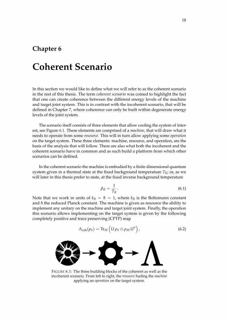


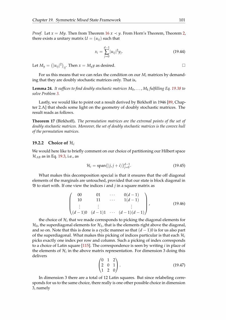


![Optimal Algebraic Manipulation Detection Codes in the Constant-Error …€¦ · Algebraic manipulation detection (AMD) codes, introduced at EUROCRYPT 2008 [5], may, in some sense,](https://static.documents.pub/doc/80x56/5f7002a91d9bb6173a100072/optimal-algebraic-manipulation-detection-codes-in-the-constant-error-algebraic-manipulation.jpg)


