1

Optimal Mechanisms for Robust Coordination inCongestion GamesPhilip N. Brown and Jason R. Marden

Abstract—Uninfluenced social systems often exhibit suboptimalperformance; specially-designed taxes can influence agent choicesand thereby bring aggregate social behavior closer to optimal.A perfect system characterization may enable a planner toapply simple taxes to incentivize desirable behavior, but sys-tem uncertainties may necessitate highly-sophisticated taxationmethodologies. Using a model of network routing, we study theeffect of system uncertainty on a designer’s ability to influencebehavior with financial incentives. We show that in principle, itis possible to design taxes that guarantee that selfish networkflows are arbitrarily close to optimal flows, despite the fact thatagents’ tax-sensitivities and network topology are unknown to thedesigner. In general, these taxes may be large; accordingly, foraffine-cost parallel-network routing games, we explicitly derivethe optimal bounded tolls and the best-possible performanceguarantee as a function of a toll upper-bound. Finally, we restrictattention to simple fixed tolls and show that they fail to providestrong performance guarantees if the designer lacks accurateinformation about network topology or user sensitivities.

I. INTRODUCTION

It is well-known that in systems that are driven by so-cial behavior, lack of coordination and agents’ self-interestedbehavior can significantly degrade system performance. Thispoor performance is commonly referred to as the price ofanarchy, defined as the ratio between the worst-case socialwelfare resulting from selfish behavior and the optimal socialwelfare [2]. This degradation of performance due to selfishbehavior has been the subject of research in areas of networkresource allocation [3], distributed control [4], traffic conges-tion [5], [6], and others. As a result, there is a growing bodyof research geared at influencing social behavior to improvesystem performance [7]–[13].

To study the issues surrounding the problem of influencingselfish social behavior, we turn to a simple model of trafficrouting: a mass of traffic needs to be routed across a networkin a way that minimizes the average network transit time. If acentral planner can direct traffic explicitly, it is straightforwardto compute the routing profile that minimizes total congestion.However, in real systems, it may not be possible to implementsuch direct centralized control or prescribe such optimalcoordinated behavior: for example, if the network represents a

Manuscript received May 2, 2016, revised November 11, 2016 and June 20,2017. This work is supported by ONR Grant #N00014-17-1-2060 and NSFGrant #ECCS-1638214.

P. N. Brown is with the Department of Electrical and Computer Engineer-ing, University of California, Santa Barbara, pnbrown@ece.ucsb.edu.Corresponding author.

J. R. Marden is with the Department of Electrical and Computer Engineer-ing, University of California, Santa Barbara, jrmarden@ece.ucsb.edu.

The conference version of this paper appeared in [1].

city’s road network, individual drivers make their own routingchoices in response to their own personal objectives.

Accordingly, we may model this routing problem as a non-atomic congestion game, where the traffic can be viewedas a collection of infinitely-many users, each controlling aninfinitesimally-small amount of traffic and seeking to minimizeits own transit time. We use the popular concept of a Nash flow(defined as a routing profile in which no user can switch to adifferent path and decrease her transit delay) to characterizethe routing profile resulting from such self-interested behavior.It is widely known that Nash flows can exhibit considerablyhigher congestion than optimal flows. An important result inthis setting states that a Nash flow on a network with generallatency functions can be arbitrarily worse than an optimalflow [14]. That is, the price of anarchy is unbounded; thisis true even on networks consisting of only two links. Recentresearch has investigated the price of anarchy of transportationnetworks under various conditions [15]–[18].

A separate research agenda has investigated methods ofincentivizing individual network users to choose more-efficientroutes, thereby aligning Nash flows with optimal flows. Thiscan be viewed as an attempt to incentivize coordinationbetween the users of the network. A natural approach to this isto charge monetary taxes for the use of network links. Existingresearch has explored methods of designing such optimal taxesgiven that the tax-designer has access to certain informationregarding the system. In [19]–[21] it is shown that optimal“fixed” taxes (i.e., taxes are constant functions of traffic flow)can be computed for any routing game, but the computationrequires precise characterizations of the network topology,user demands, and user tax-sensitivities. In contrast, [22],[23] derive optimal taxes known as “marginal-cost taxes”which require no knowledge of the network topology or userdemands, but require that all users share a common known tax-sensitivity. Furthermore, the marginal-cost taxation functionsmust be strictly flow-varying. Section III details these results.

In this paper, we ask if it is possible to compute optimaltaxes with minimal information about the system, and presentseveral new results showcasing the relationship between avail-able tolling methodologies, uncertainty, and achievable perfor-mance. We term this goal “robust coordination,” as we desireto incentivize agents to behave as though they are coordinatingwith one another, but we require that our behavior-influencingmechanisms are robust to mischaracterizations of the system.Since price of anarchy is simply a cost metric in worst-caseover some set of unknown information, it lends itself naturallyto quantifying the robustness of taxation mechanisms to un-known information. Thus, our analysis represents a departure

2

both from the typical descriptive price of anarchy researchas well as from the complete-information assumptions of thetaxation literature.

Our main contribution is to derive a universal taxationmechanism that guarantees arbitrarily-good performance forany routing game while requiring no prior knowledge of thespecific network, user demand profile, or distribution of usersensitivities. That is, our derived taxes are robust to grossmischaracterizations of the above quantities. This result holdsfor networks with general latency functions and any topology,suggesting that surprisingly-little information is required inprinciple.

Our next result explores the effect of reducing the designer’scapabilities while maintaining a high level of uncertainty. Tothis end, our second contribution is to explore the effect ofplacing an upper bound on the allowable tolling functions.This may have practical value in settings where very large tollsmay be impossible (or politically unpalatable) to implement.For parallel networks with linear-affine latency functions, wederive the optimal tolling functions that minimize worst-case performance degradation for any unknown distributionof user sensitivities and toll upper bound, requiring no priorknowledge of the number of network links. These optimaltolls are simple affine functions of flow. We show that forparallel networks with linear-affine cost functions and simpleuser demands, the worst-case performance degradation strictlydecreases with the toll upper bound. Our results suggestthat large tolls can compensate for a poor characterizationof user sensitivities. Unfortunately, by imposing an upperbound on allowable taxation functions, optimal behavior canno longer be guaranteed. Thus, this result additionally impliesthat unbounded tolls are necessary to enforce optimal flows ifboth the network topology and user sensitivities are unknown.

Our results in Section VI explore a further restriction onthe designer’s capabilities, requiring that tolls do not dependon flow (i.e., requiring fixed tolls rather than tolling func-tions). These results suggest that fixed tolls lack robustness tomischaracterizations of network topology and user sensitivity.First, if the network topology is unknown, fixed tolls cannotenforce perfectly optimal routing, and we present a simplesetting in which network performance can be arbitrarily bad iffixed tolls are not allowed to depend on the network structure.Finally, we show that even if fixed tolls are allowed to dependon the network topology and user demands, they providerelatively poor performance guarantees when the user sensitiv-ities are unknown. Here, by reducing the designer’s capability(by disallowing access to flow-varying taxation functions), wedramatically reduce the achievable performance guarantees inthe presence of uncertainty. That is, fixed tolls are significantlyless robust than flow-varying tolls. Our negative result herevividly demonstrates the need for a clear understanding of therobustness of incentive mechanisms to model imperfections.

II. MODEL AND PERFORMANCE METRICS

A. Routing Game

Consider a network routing problem in which a unit massof traffic needs to be routed across a network (V,E), which

consists of a vertex set V and edge set E ⊆ (V ×V ). We call asource/destination vertex pair (sc, tc) ∈ (V ×V ) a commodity,and the set of all such commodities C. For each c ∈ C, thereis a mass of traffic rc > 0 that needs to be routed from sc totc. We write Pc ⊂ 2E to denote the set of paths available totraffic in commodity c, where each path p ∈ Pc consists of aset of edges connecting sc to tc. Let P = ∪{Pc}.

We write f cp ≥ 0 to denote the mass of traffic fromcommodity c using path p, and fp ,

∑c∈C f

cp . A feasible flow

f ∈ R|P| is an assignment of traffic to various paths such thatfor each c,

∑p∈Pc f cp = rc. Without loss of generality, we

assume that∑c∈C r

c = 1.Given a flow f , the flow on edge e is given by fe =∑p:e∈p fp. To characterize transit delay as a function of traffic

flow, each edge e ∈ E is associated with a specific latencyfunction `e : [0, 1] → [0,∞). We adopt the standard assump-tions that latency functions are nondecreasing, continuouslydifferentiable, and convex. Note that latency functions areanonymous: all traffic affects delay equally. The cost of a flowf is measured by the total latency, given by

L(f) =∑e∈E

fe · `e(fe) =∑p∈P

fp · `p(fp), (1)

where `p(f) =∑e∈p `e(fe) denotes the latency on path p.

We denote the flow that minimizes the total latency by

f∗ ∈ argminf is feasible

L(f). (2)

A routing problem is given by the tuple G = (V,E, C, {`e}).We write the set of all such routing problems as G, and oftenwrite e ∈ G to denote (e ∈ G : G ∈ G).

In this paper we study taxation mechanisms for influencingthe emergent collective behavior resulting from self-interestedprice-sensitive users. To that end, we model the above routingproblem as a non-atomic game in which the traffic modelsa large population of users. Thus, we use the terms “traffic,”“users,” and “agents” interchangeably. We assign each edge1

e ∈ E a flow-dependent, nondecreasing taxation functionτe : [0, 1] → R+. We characterize the taxation sensitivitiesof the users in commodity c with a monotone, nondecreasingfunction sc : [0, rc] → [SL, SU], where each user x ∈ [0, rc]has a taxation sensitivity scx ∈ [SL, SU] ⊆ R+ and SU ≥ SL ≥0 denote upper and lower sensitivity bounds, respectively.Given a flow f , the cost that user x ∈ [0, rc] experiencesfor using path p ∈ Pc is of the form

Jcx(f) =∑e∈p

[`e(fe) + scxτe(fe)] . (3)

Thus, for each user x ∈ [0, rc], the sensitivity scx can be viewedas a constant gain on the toll; a user’s experienced cost is thenthe sum of the latency and sensitivity-weighted toll. Note thatsensitivity can be interpreted as the reciprocal of an agent’svalue-of-time.2 Note that scx need not equal scy for x 6= y. We

1Note that we allow all edges to be taxed (as in [19]–[23]); see [24] for arelaxation of this requirement.

2We adopt this formulation from [19]. Note that constant sensitivity is acommonly-studied special case; alternative formulations are possible [25].

3

assume that each user prefers the lowest-cost path from theavailable source-destination paths. We call a flow f a Nashflow if for all commodities c ∈ C and all users x ∈ [0, rc] wehave

Jcx(f) = minp∈Pc

{∑e∈p

[`e(fe) + scxτe(fe)]

}. (4)

It is well-known that a Nash flow exists for any non-atomicgame of the above form [26].

In our analysis, we assume that each sensitivity distributionfunction sc is unknown; for a given routing problem G andSU ≥ SL ≥ 0 we define the set of possible sensitivitydistributions as the set of monotone, nondecreasing functionsSG = {sc : [0, rc] → [SL, SU]}c∈C . We write s ∈ SG todenote such a specific collection of sensitivity distributions,which we term a population.

B. Price of Anarchy and Robustness

For a given routing problem G ∈ G, we gauge the efficacy ofa collection of taxation functions τ = {τe}e∈E by comparingthe total latency of the resulting Nash flow and the total latencyassociated with the optimal flow, and then performing a worst-case analysis over all possible user populations. Let L∗(G)denote the total latency associated with the optimal flow, andLnf(G, s, τ) denote the total latency of the worst-performingNash flow resulting from taxation functions τ and populations. The worst-case system cost associated with this specificinstance is captured by the price of anarchy which is of theform

PoA(G, τ) = sups∈SG

{Lnf (G, s, τ)

L∗(G)

}≥ 1. (5)

In this context, we seek taxation mechanisms which mini-mize PoA(G, τ) for a wide variety of routing games G. If ataxation mechanism τ brings PoA(G, τ) close to 1 for manygames G (in a sense to be made exact later), this indicatesthat τ is robust to to mischaracterizations of user sensitivities.Traditionally, the price of anarchy is analyzed in worst caseover a given class of games [14]. In our usage, we delay takingthe worst case over all networks until specific settings whenit is called for. For example, Theorem 1 exhibits a taxationmechanism which drives the price of anarchy to 1 for everyG, but the rate at which the price of anarchy approaches 1 mayvary from network to network. On the other hand, Theorem 3provides an expression for the price of anarchy that holds forall parallel networks.

III. RELATED WORK

The following is a brief overview of the existing literatureon taxation mechanisms in this context. A taxation mechanismsimply computes edge tolls as a function of some set ofinformation about the system; here, we focus in particularon the informational dependencies of several well-studiedtaxation approaches.– Omniscient taxation mechanisms: These taxation mecha-nisms are assumed to have access to complete informationregarding the routing game. For edge e ∈ G and populations ∈ SG, the edge tolling function takes the following form:

τe (fe;G, s) . That is, each edge’s taxation function can dependon the entire routing problem G and the population sensi-tivities s. Recent results have identified taxation mechanismsof this form that assign fixed tolls (i.e., for any e ∈ G,τe(fe) = qe for some qe ≥ 0) that can enforce any feasibleflow [20], [21], thus guaranteeing a price of anarchy of 1.However, the robustness of these mechanisms to variations ormischaracterizations of network topology and user sensitivitiesis heretofore unknown.– Network-agnostic taxation mechanisms: This type of tax-ation mechanism is agnostic to network specifications: eachtaxation function is derived from locally-available informationonly. Here, a system designer essentially commits to a taxationfunction for each potential edge e ∈ G, and any networkrealization G ∈ G merely employs a subset of these pre-defined taxation functions. An edge’s toll cannot depend onany other edge’s cost or location in the network, nor can itdepend on the tax-sensitivities of the agents.

A commonly-studied network-agnostic taxation mecha-nisms is the marginal-cost (or Pigovian) taxation mechanismτmc, which is of the following form: for any e ∈ G withlatency function `e, the accompanying taxation function is

τmce (fe) = fe ·

d

dfe`e(fe), ∀fe ≥ 0. (6)

In [22] it is shown that for any G ∈ G we have L∗(G) =Lnf (G, s, τmc) provided that all users have a sensitivity ex-actly equal to 1. Hence, irrespective of the underlying networkstructure, a marginal-cost taxation mechanism always ensuresthe optimality of the resulting Nash flow, provided that allusers share a common known sensitivity.

There are many other results in this area; for example,in [27] the authors investigate the price of anarchy of varioustypes of tolling functions with built-in upper bounds. In [28],it is shown that if taxes can be computed in a centralizedfashion, any feasible flow can be enforced even if the centralplanner does not know the network’s latency functions. Foraffine-cost parallel networks, [29] derives omniscient, flow-varying taxation mechanisms for applications where the totaltraffic rate is unknown. Finally, in [7], the authors show thatmarginal-cost taxes scaled by

√SLSU do possess a degree

of robustness to mischaracterizations of user sensitivities foraffine-cost parallel networks.

IV. A UNIVERSAL TAXATION MECHANISM

In this paper, we prove that network- and sensitivity-agnostic tolls exist which can drive the price of anarchy to1 for general networks and latency functions. We term these“universal” because they take the same form and provide thesame performance guarantee regardless of which particularrouting scenario they are applied to. Using this taxation mech-anism, we show in Theorem 1 that for any network, regardlessof network topology, traffic rates {rc}, or price-sensitivityfunctions {sc}, the price of anarchy can be made arbitrarilyclose to 1 with sufficiently-large edge tolls, indicating thattolls exist which are robust to mischaracterizations of all theaforementioned system parameters.

4

Theorem 1. Let G be the set of multi-commodity routinggames where SU ≥ SL > 0. For any network edge e ∈ Gwith convex, nondecreasing, continuously differentiable la-tency function `e, define the universal taxation function onedge e with gain parameter κ ≥ 0 as

τue (fe;κ) = κ

(`e(fe) + fe ·

d

dfe`e(fe)

). (7)

Then for any routing problem G ∈ G,

limκ→∞

PoA (G, τu(κ)) = 1. (8)

That is, on any network being used by any populationof users, the total latency can be made arbitrarily close tothe optimal latency, and each individual link toll is a simplecontinuous function of that link’s flow. The reason for this isthat as κ increases, the original latency function has a smallerand smaller relative effect on the users’ cost functions; in thelarge-toll limit, the only cost experienced by the users is thetolling function itself which is specifically designed to induceoptimal Nash flows.

Proof. Using a sequence of tolls, we construct a sequence ofNash flows that converges to an optimal flow. Let κn be anunbounded, increasing sequence of tolling coefficients.

For any routing problem G ∈ G and price-sensitivities s ∈SG, let fn =

(fnp)p∈P denote the Nash flow resulting from

the tolling coefficient κn. For each commodity c, let Pcn ⊆ Pcdenote the set of paths that have positive flow in fn. For anyp ∈ Pcn, there must be some user x ∈ [0, rc] using p withsensitivity scx; the cost experienced by this user is given by

Jcx(fn) =∑e∈p

[`e(fe) + κns

cx

(`e(fe) + fe ·

d

dfe`e(fe)

)].

Define γn,x , κnscx

1+κnscx. Let `∗e(fe) = fe · d

dfe`e(fe); then for

any other path p′ ∈ Pc \ p, user x must experience a lowercost on p than on p′, or∑e∈p

`e(fe)−∑e∈p′

`e(fe) ≤ γn,x

∑e∈p′

`∗e(fe)−∑e∈p

`∗e(fe)

. (9)

Therefore, for any n ≥ 1, fn must satisfy some set ofinequalities defined by (9). Note that for all c ∈ C and anyx ∈ [0, rc], limκn→∞ γn,x = 1, so because all the functionsin (9) are continuous, fn converges to a set F ∗ of feasibleflows that satisfy∑e∈p

`e(fe)−∑e∈p′

`e(fe) ≤

∑e∈p′

`∗e(fe)−∑e∈p

`∗e(fe)

(10)

for all c, all p ∈ Pc∗, and p′ ∈ Pc, where Pc∗ ⊆ Pc issome subset of paths. But inequalities (10) (combined withthe feasibility constraints on f ) also specify a Nash flow forG for a unit-sensitivity population with marginal-cost taxes asspecified by (6). Any such Nash flow must be optimal [22];that is, any f ∈ F ∗ is a minimum-latency flow for G. Thus,since L(f) is a continuous function of f ,

limn→∞

L (fn) = L∗ (G) , (11)

obtaining the proof of the theorem.

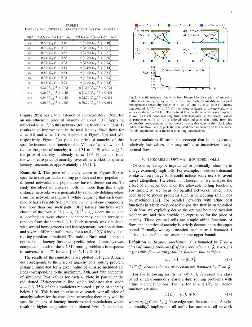
Fig. 1. Base network for Examples 1 and 2. This network has threecommodities (i.e., source-destination pairs): (A,B) (red), (A,E) (green),and (C,D) (blue), with associated traffic rates r1, r2, and r3, respectively.Traffic in each commodity has access to all directed paths that connect therespective source and destination; for example, (A,B) can choose between{e1}, {e2, e3, e4}, and {e2, e7, e8}. For a demonstration of universal tollsapplied to a specific instance of this network, see Figure 2. To demonstrate theeffects of the universal tolls of Theorem 1, random variations of this networkare simulated and the resulting price-of-anarchy values are plotted in Figure 3.

A. Price of Anarchy Bounds for Homogeneous Populations

The result in Theorem 1 is encouraging since it ensuresthat no routing game or user population is so pathologicalthat we cannot enforce optimal routing with sufficiently-high tolls, but it gives no indication of how high these tollsmust be. In our next result in Proposition 2 (which followsfrom a result in [30]), we state that for homogeneous price-sensitive populations (i.e., all users have the same non-zeroprice sensitivity), the performance degradation is uniformlybounded in all games by a simple expression.

Proposition 2. If all users have (unknown) homogeneousprice-sensitivity s ≥ SL > 0, the price of anarchy inducedby τu(κ) is given by

supG∈G

PoA (G, τu(κ)) ≤ 1 + κSL

κSL. (12)

Proof. Immediate from Proposition 6.4 of [30].

B. Examples Illustrating Universal Tolls

Example 1. Consider the network in Figure 1. This net-work has been used to demonstrate dynamic tolling mecha-nisms [13], and we use variations of it to illustrate the universaltolls of Theorem 1. This network has three commodities,labeled in Figure 1 as (A,B) (red), (A,E) (green), and (C,D)(blue), with respective traffic rates r1, r2, and r3. Traffic ineach commodity has access to all paths connecting its sourceto its destination; for example, the (A,B) commodity (shownin red in Figure 1) has access to three paths: {e1}, {e2, e3, e4},and {e2, e7, e8}.

First, consider an instance of this network in which r1 =r2 = r3 = 0.5, all traffic in commodity 1 has sensitivitys1 = 100, and all traffic in commodities 2 and 3 havesensitivity s2 = s3 = 0.1. Let the latency functions begiven by `e(fe) = ae (fe)

4+ be, with coefficients ae and

be given in Table I. Quartic latency functions of this formare a stylized form of the well-known Bureau of PublicRoads (BPR) latency functions, commonly used to modelthe congestion characteristics of physical roads [13], [31].The optimal flow on this network (Figure 2(a)) has a totallatency of approximately 1.49; the un-influenced Nash flow

5

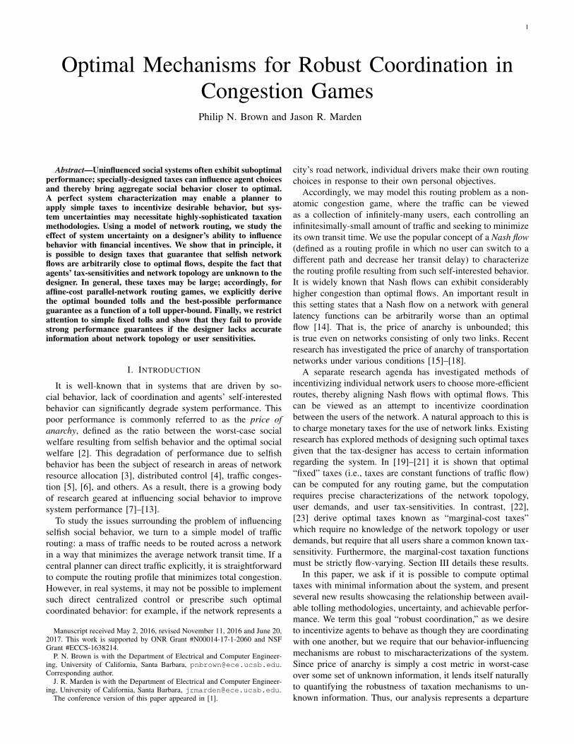
TABLE ILATENCY AND UNIVERSAL TOLLING FUNCTIONS FOR EXAMPLE 1

edge `e(fe) = ae(fe)4 + be τue (fe) = κ(5ae(fe)4 + be

)e1 0.88(fe1 )4 + 0.10 κ

(4.40(fe1 )4 + 0.10

)e2 0.59(fe2 )4 + 0.91 κ

(2.95(fe2 )4 + 0.91

)e3 0.66(fe3 )4 + 0.87 κ

(3.30(fe3 )4 + 0.87

)e4 0.24(fe4 )4 + 0.88 κ

(1.20(fe4 )4 + 0.88

)e5 0.57(fe5 )4 + 0.93 κ

(2.85(fe5 )4 + 0.93

)e6 0.62(fe6 )4 + 0.12 κ

(3.10(fe6 )4 + 0.12

)e7 0.89(fe7 )4 + 0.34 κ

(4.45(fe7 )4 + 0.34

)e8 0.93(fe8 )4 + 0.93 κ

(4.65(fe8 )4 + 0.93

)e9 0.68(fe9 )4 + 0.22 κ

(3.40(fe9 )4 + 0.22

)e10 0.31(fe10 )4 + 0.72 κ

(1.55(fe10 )4 + 0.72

)e11 0.26(fe11 )4 + 0.40 κ

(1.30(fe11 )4 + 0.40

)e12 0.54(fe12 )4 + 0.45 κ

(2.70(fe12 )4 + 0.45

)e13 0.06(fe13 )4 + 0.08 κ

(0.30(fe13 )4 + 0.08

)

(Figure 2(b)) has a total latency of approximately 1.955, foran un-influenced price of anarchy of about 1.31. Applyinguniversal tolls (7) to this network (tolling functions in Table I)results in an improvement in the total latency; Nash flows forκ = 0.5 and κ = 10 are depicted in Figure 2(c) and (d),respectively. Figure 2(e) plots the price of anarchy of thisspecific instance as a function of κ. Values of κ as low as 0.1reduce the price of anarchy from 1.31 to 1.19; when κ ≥ 5,the price of anarchy is already below 1.05. For comparison,the worst-case price of anarchy (over all networks) for quarticlatency functions is approximately 2.15 [14].

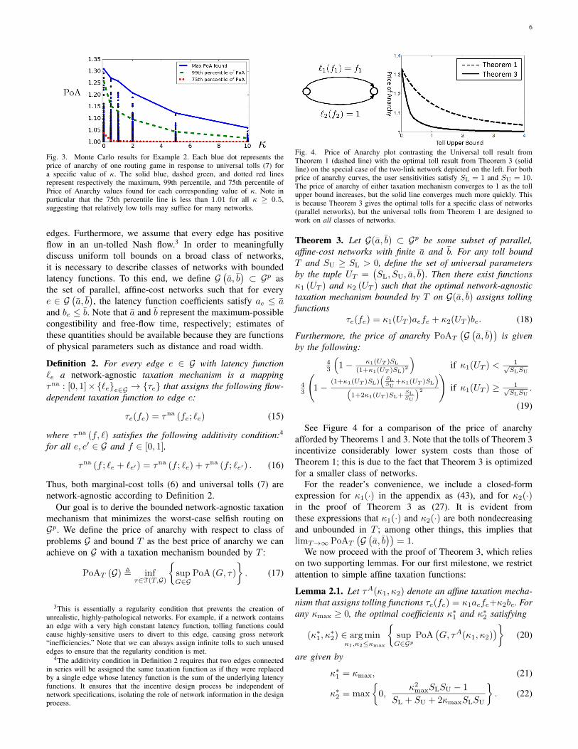
Example 2. The price of anarchy curve in Figure 2(e) isspecific to one particular routing problem and user population;different networks and populations have different curves. Tostudy the effect of universal tolls on more than this singleinstance, networks were generated by randomly deleting edgesfrom the network in Figure 1 (while requiring that each com-modity has a feasible S-D path and that at least one commodityhas more than one such path). BPR latency functions werechosen of the form `e(fe) = ae (fe)

4+ be, where the ae and

be coefficients were chosen independently and uniformly atrandom from the interval [0, 1]. Each network was simulatedwith several homogeneous and heterogeneous user populationsand several different traffic rates, for a total of 2,314 individualrouting problems simulated. The ratio of Nash total latency tooptimal total latency (instance-specific price of anarchy) wascomputed on each of these 2,314 routing problems in responseto universal tolls (7) for κ ∈ {0, 0.5, 1, 2, 5, 10}.

The results of the simulations are plotted in Figure 3. Eachdot corresponds to the price of anarchy of a routing probleminstance simulated for a given value of κ. Also included arelines corresponding to the maximum, 99th, and 75th percentileof simulated PoA values for each κ. Note in particular thered dotted 75th-percentile line which indicates that whenκ = 0.5, 75% of the simulations reported a price of anarchybelow 1.01. This is not an exhaustive search over all price ofanarchy values for the considered networks; there may well bespecific choices of latency functions and populations whichresult in higher congestion than plotted here. Nonetheless,

Fig. 2. Specific instance of network from Figure 1 for Example 1. Commoditytraffic rates are r1 = r2 = r3 = 0.5, and each commodity is assignedhomogeneous sensitivity values of s1 = 100 and s2 = s3 = 0.1. Latencyfunctions of `e(fe) = ae (fe)4 + be were assigned to the network, withvalues as shown in Table I. The optimal flow on the network was computed,as well as Nash flows resulting from universal tolls (7) for several valuesof parameter κ. In (a)-(d), a colored edge indicates that traffic from thecommodity corresponding to that color is using that edge; a thin black edgeindicates no flow. Part (e) plots the simulated price of anarchy on this network,for this population, as a function of tolling parameter κ.

these simulations illustrate the concept that in many cases,relatively low values of κ may suffice to incentivize nearly-optimal flows.

V. THEOREM 3: OPTIMAL BOUNDED TOLLS

Of course, it may be impractical or politically infeasible tocharge extremely high tolls. For example, if network demandis elastic, very large tolls could induce some users to avoidtravel altogether. Therefore, in Theorem 3, we analyze theeffect of an upper bound on the allowable tolling functions.For simplicity, we focus on parallel networks, which havebeen used to model problems such as scheduling small jobson machines [32]. For parallel networks with affine costfunctions in which every edge has positive flow in an un-tolledNash flow, we explicitly derive the optimal bounded taxationmechanism, and then provide an expression for the price ofanarchy. These optimal tolls are simple affine functions offlow, and the price of anarchy is strictly decreasing in the upperbound. Formally, we say a taxation mechanism is bounded ifall its taxation functions respect some upper bound:

Definition 1. Taxation mechanism τ is bounded by T on aclass of routing problems G if for every edge e ∈ G, τ assignsa (possibly flow-varying) tolling function that satisfies

τe : [0, 1]→ [0, T ]. (13)

T(T, G

)denotes the set of mechanisms bounded by T on G.

For the following results, let Gp ⊆ G represent the classof all single-commodity, parallel-link routing problems withaffine latency functions. That is, for all e ∈ Gp, the latencyfunction satisfies

`e(fe) = aefe + be (14)

where ae ≥ 0 and be ≥ 0 are edge-specific constants. “Single-commodity” implies that all traffic has access to all network

6

Fig. 3. Monte Carlo results for Example 2. Each blue dot represents theprice of anarchy of one routing game in response to universal tolls (7) fora specific value of κ. The solid blue, dashed green, and dotted red linesrepresent respectively the maximum, 99th percentile, and 75th percentile ofPrice of Anarchy values found for each corresponding value of κ. Note inparticular that the 75th percentile line is less than 1.01 for all κ ≥ 0.5,suggesting that relatively low tolls may suffice for many networks.

edges. Furthermore, we assume that every edge has positiveflow in an un-tolled Nash flow.3 In order to meaningfullydiscuss uniform toll bounds on a broad class of networks,it is necessary to describe classes of networks with boundedlatency functions. To this end, we define G

(a, b)⊂ Gp as

the set of parallel, affine-cost networks such that for everye ∈ G

(a, b), the latency function coefficients satisfy ae ≤ a

and be ≤ b. Note that a and b represent the maximum-possiblecongestibility and free-flow time, respectively; estimates ofthese quantities should be available because they are functionsof physical parameters such as distance and road width.

Definition 2. For every edge e ∈ G with latency function`e a network-agnostic taxation mechanism is a mappingτna : [0, 1]×{`e}e∈G → {τe} that assigns the following flow-dependent taxation function to edge e:

τe(fe) = τna (fe; `e) (15)

where τna (f, `) satisfies the following additivity condition:4

for all e, e′ ∈ G and f ∈ [0, 1],

τna (f ; `e + `e′) = τna (f ; `e) + τna (f ; `e′) . (16)

Thus, both marginal-cost tolls (6) and universal tolls (7) arenetwork-agnostic according to Definition 2.

Our goal is to derive the bounded network-agnostic taxationmechanism that minimizes the worst-case selfish routing onGp. We define the price of anarchy with respect to class ofproblems G and bound T as the best price of anarchy we canachieve on G with a taxation mechanism bounded by T :

PoAT (G) , infτ∈T(T,G)

{supG∈G

PoA (G, τ)

}. (17)

3This is essentially a regularity condition that prevents the creation ofunrealistic, highly-pathological networks. For example, if a network containsan edge with a very high constant latency function, tolling functions couldcause highly-sensitive users to divert to this edge, causing gross network“inefficiencies.” Note that we can always assign infinite tolls to such unusededges to ensure that the regularity condition is met.

4The additivity condition in Definition 2 requires that two edges connectedin series will be assigned the same taxation function as if they were replacedby a single edge whose latency function is the sum of the underlying latencyfunctions. It ensures that the incentive design process be independent ofnetwork specifications, isolating the role of network information in the designprocess.

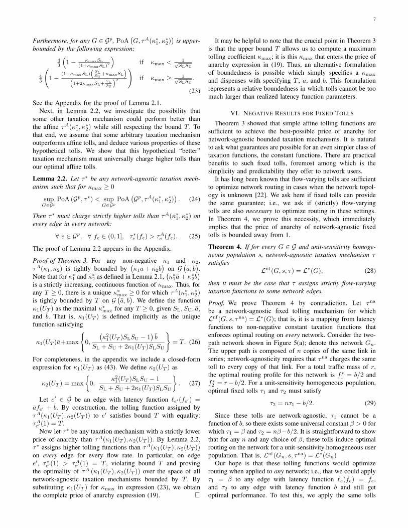
Fig. 4. Price of Anarchy plot contrasting the Universal toll result fromTheorem 1 (dashed line) with the optimal toll result from Theorem 3 (solidline) on the special case of the two-link network depicted on the left. For bothprice of anarchy curves, the user sensitivities satisfy SL = 1 and SU = 10.The price of anarchy of either taxation mechanism converges to 1 as the tollupper bound increases, but the solid line converges much more quickly. Thisis because Theorem 3 gives the optimal tolls for a specific class of networks(parallel networks), but the universal tolls from Theorem 1 are designed towork on all classes of networks.

Theorem 3. Let G(a, b) ⊂ Gp be some subset of parallel,affine-cost networks with finite a and b. For any toll boundT and SU ≥ SL > 0, define the set of universal parametersby the tuple UT =

(SL, SU, a, b

). Then there exist functions

κ1 (UT ) and κ2 (UT ) such that the optimal network-agnostictaxation mechanism bounded by T on G(a, b) assigns tollingfunctions

τe(fe) = κ1(UT )aefe + κ2(UT )be. (18)

Furthermore, the price of anarchy PoAT

(G(a, b))

is givenby the following:

43

(1− κ1(UT )SL

(1+κ1(UT )SL)2

)if κ1(UT ) < 1√

SLSU

43

(1−

(1+κ1(UT )SL)(

SLSU

+κ1(UT )SL

)(1+2κ1(UT )SL+

SLSU

)2

)if κ1(UT ) ≥ 1√

SLSU.

(19)

See Figure 4 for a comparison of the price of anarchyafforded by Theorems 1 and 3. Note that the tolls of Theorem 3incentivize considerably lower system costs than those ofTheorem 1; this is due to the fact that Theorem 3 is optimizedfor a smaller class of networks.

For the reader’s convenience, we include a closed-formexpression for κ1(·) in the appendix as (43), and for κ2(·)in the proof of Theorem 3 as (27). It is evident fromthese expressions that κ1(·) and κ2(·) are both nondecreasingand unbounded in T ; among other things, this implies thatlimT→∞ PoAT

(G(a, b))

= 1.We now proceed with the proof of Theorem 3, which relies

on two supporting lemmas. For our first milestone, we restrictattention to simple affine taxation functions:

Lemma 2.1. Let τA(κ1, κ2) denote an affine taxation mecha-nism that assigns tolling functions τe(fe) = κ1aefe+κ2be. Forany κmax ≥ 0, the optimal coefficients κ∗1 and κ∗2 satisfying

(κ∗1, κ∗2) ∈ arg min

κ1,κ2≤κmax

{supG∈Gp

PoA(G, τA(κ1, κ2)

)}(20)

are given by

κ∗1 = κmax, (21)

κ∗2 = max

{0,

κ2maxSLSU − 1

SL + SU + 2κmaxSLSU

}. (22)

7

Furthermore, for any G ∈ Gp, PoA(G, τA(κ∗1, κ

∗2))

is upper-bounded by the following expression:

43

(1− κmaxSL

(1+κmaxSL)2

)if κmax <

1√SLSU

43

(1−

(1+κmaxSL)(

SLSU

+κmaxSL

)(1+2κmaxSL+

SLSU

)2

)if κmax ≥ 1√

SLSU.

(23)

See the Appendix for the proof of Lemma 2.1.Next, in Lemma 2.2, we investigate the possibility that

some other taxation mechanism could perform better thanthe affine τA(κ∗1, κ

∗2) while still respecting the bound T . To

that end, we assume that some arbitrary taxation mechanismoutperforms affine tolls, and deduce various properties of thesehypothetical tolls. We show that this hypothetical “better”taxation mechanism must universally charge higher tolls thanour optimal affine tolls.

Lemma 2.2. Let τ∗ be any network-agnostic taxation mech-anism such that for κmax ≥ 0

supG∈Gp

PoA (Gp, τ∗) < supG∈Gp

PoA(Gp, τA(κ∗1, κ

∗2)). (24)

Then τ∗ must charge strictly higher tolls than τA(κ∗1, κ∗2) on

every edge in every network:

∀ e ∈ Gp, ∀ fe ∈ (0, 1], τ∗e (fe) > τAe (fe). (25)

The proof of Lemma 2.2 appears in the Appendix.

Proof of Theorem 3. For any non-negative κ1 and κ2,τA(κ1, κ2) is tightly bounded by

(κ1a+ κ2b

)on G

(a, b).

Note that for κ∗1 and κ∗2 as defined in Lemma 2.1,(κ∗1a+ κ∗2b

)is a strictly increasing, continuous function of κmax. Thus, forany T ≥ 0, there is a unique κ∗max ≥ 0 for which τA(κ∗1, κ

∗2)

is tightly bounded by T on G(a, b). We define the function

κ1(UT ) as the maximal κ∗max for any T ≥ 0, given SL, SU, a,and b. That is, κ1(UT ) is defined implicitly as the uniquefunction satisfying

κ1(UT )a+max

{0,

(κ21(UT )SLSU − 1

)b

SL + SU + 2κ1(UT )SLSU

}= T. (26)

For completeness, in the appendix we include a closed-formexpression for κ1(UT ) as (43). We define κ2(UT ) as

κ2(UT ) = max

{0,

κ21(UT )SLSU − 1

SL + SU + 2κ1(UT )SLSU

}. (27)

Let e′ ∈ G be an edge with latency function `e′(fe′) =afe′ + b. By construction, the tolling function assigned byτA(κ1(UT ), κ2(UT )) to e′ satisfies bound T with equality:τAe′ (1) = T .

Now let τ∗ be any taxation mechanism with a strictly lowerprice of anarchy than τA(κ1(UT ), κ2(UT )). By Lemma 2.2,τ∗ assigns higher tolling functions than τA(κ1(UT ), κ2(UT ))on every edge for every flow rate. In particular, on edgee′, τ∗e′(1) > τAe′ (1) = T , violating bound T and provingthe optimality of τA (κ1(UT ), κ2(UT )) over the space of allnetwork-agnostic taxation mechanisms bounded by T . Bysubstituting κ1(UT ) for κmax in expression (23), we obtainthe complete price of anarchy expression (19).

It may be helpful to note that the crucial point in Theorem 3is that the upper bound T allows us to compute a maximumtolling coefficient κmax; it is this κmax that enters the price ofanarchy expression in (19). Thus, an alternative formulationof boundedness is possible which simply specifies a κmax

and dispenses with specifying T , a, and b. This formulationrepresents a relative boundedness in which tolls cannot be toomuch larger than realized latency function parameters.

VI. NEGATIVE RESULTS FOR FIXED TOLLS

Theorem 3 showed that simple affine tolling functions aresufficient to achieve the best-possible price of anarchy fornetwork-agnostic bounded taxation mechanisms. It is naturalto ask what guarantees are possible for an even simpler class oftaxation functions, the constant functions. There are practicalbenefits to such fixed tolls, foremost among which is thesimplicity and predictability they offer to network users.

It has long been known that flow-varying tolls are sufficientto optimize network routing in cases when the network topol-ogy is unknown [22]. We ask here if fixed tolls can providethe same guarantee; i.e., we ask if (strictly) flow-varyingtolls are also necessary to optimize routing in these settings.In Theorem 4, we prove this necessity, which immediatelyimplies that the price of anarchy of network-agnostic fixedtolls is bounded away from 1.

Theorem 4. If for every G ∈ G and unit-sensitivity homoge-neous population s, network-agnostic taxation mechanism τsatisfies

Lnf(G, s, τ) = L∗(G), (28)

then it must be the case that τ assigns strictly flow-varyingtaxation functions to some network edges.

Proof. We prove Theorem 4 by contradiction. Let τna

be a network-agnostic fixed tolling mechanism for whichLnf(G, s, τna) = L∗(G); that is, it is a mapping from latencyfunctions to non-negative constant taxation functions thatenforces optimal routing on every network. Consider the two-path network shown in Figure 5(a); denote this network Gn.The upper path is composed of n copies of the same link inseries; network-agnosticity requires that τna charges the sametoll to every copy of that link. For a total traffic mass of r,the optimal routing profile for this network is f∗1 = b/2 andf∗2 = r− b/2. For a unit-sensitivity homogeneous population,optimal fixed tolls τ1 and τ2 must satisfy

τ2 = nτ1 − b/2. (29)

Since these tolls are network-agnostic, τ1 cannot be afunction of b, so there exists some universal constant β > 0 forwhich τ1 = β and τ2 = nβ−b/2. It is straightforward to showthat for any n and any choice of β, these tolls induce optimalrouting on the network for a unit-sensitivity homogeneous userpopulation. That is, Lnf(Gn, s, τ

na) = L∗(Gn)Our hope is that these tolling functions would optimize

routing when applied to any network; i.e., that we could applyτ1 = β to any edge with latency function `e(fe) = fe,and τ2 to any edge with latency function b and still getoptimal performance. To test this, we apply the same tolls

8

Fig. 5. Networks for Theorem 4 Proof. In both networks, `1(f1) = f1and `2(f2) = b, with b > 0. (a): Network with n copies of the same linkin series on the upper path. Since every upper edge has the same latencyfunction, network-agnostic tolls must charge the same amount to each edge.(b): The same network with n = 1; if network-agnostic tolls τ1 and τ2 weredesigned for network (a), they can cause highly inefficient performance onnetwork (b).

to the network in Figure 5(b), which we denote G1. Here,we find that τ2 = nβ − b/2 is now much too high; if thetotal traffic rate is high enough, these tolls induce a flow withf1 = β(n − 1) + b/2 and f2 = 0, even though the optimalflow has f1 = b/2. This allows us to compute a lower boundon the price of anarchy for these tolling functions:

Lnf(G1, s, τna)

L∗(G1)≥(β(n− 1) + b

2

)2b(β(n− 1) + b

4

) , (30)

which is unbounded in both n and β, generating a contractionto our hypothesis that for all G, Lnf(G, s, τna) = L∗(G).

In light of this negative result, in Theorem 5, we ask whatguarantees are possible with fixed tolls if we know the networkstructure but do not know the user sensitivities; refer to thelast row of Table II for a quick summary of the setting weinvestigate here. Since we are allowing these fixed tolls todepend on network structure (e.g., the number of edges inthe network), we denote such taxation functions by τ ft(G) ={τ fte (G)}e∈G. The following theorem demonstrates that anynetwork-dependent fixed-toll taxation mechanism generallyprovides poor performance guarantees when compared withthe optimal bounded taxation mechanism from Theorem 3.

Theorem 5. Consider any network-dependent fixed-toll taxa-tion mechanism τ ft. For any network G ∈ Gp,

sups∈SLnf

(G, s, τ ft(G)

)≥ sup

s∈SLnf

(G, s, τA(1/SU, 0)

), (31)

with affine tolls τA(·) as defined in Lemma 2.1. Thus,

supG∈G

PoA(G, τ ft

)≥ supG∈Gp

PoA(G, τA(1/SU, 0)

)=

4

3

(1− SL/SU

(1 + SL/SU)2

). (32)

We point out that the right-hand side of (32) representsthe price of anarchy due to network-agnostic affine tolls fora very low toll upper bound. For example, in the canonicalPigou network depicted in Figure 4, if SU = 10, affine tollsprescribed by τA(1/SU, 0) imply a toll upper-bound of just0.1. As shown in Figure 4, the price of anarchy for optimalaffine tolls is steeply decreasing in the toll upper-bound, so adesigner wishing to exploit the simplicity of fixed tolls mayneed to accept lower performance guarantees as a result.

Furthermore, it is important to note that Theorem 5 showsthat τA, a network-agnostic tolling mechanism, provides betterperformance guarantees (even for moderately low tolls) than

Fig. 6. Comparison of Price of Anarchy guaranteed by Theorems 3 and 5. Allplots are for SL = 1 and a = b = 1. The horizontal axis represents the levelof certainty in price-sensitivity; note that most taxation mechanisms guaranteea price of anarchy of 1 for complete certainty unless they are restricted by avery low upper-bound. The solid line represents the price of anarchy resultingfrom fixed tolls (according to (32)), and the marked lines represent the priceof anarchy resulting from optimal flow-varying affine tolls for a given tollbound (according to (19)). Note that for a very low toll bound, fixed tollsslightly outperform affine tolls for well-characterized populations; this is dueto the fact that the fixed tolls are not restricted by the toll upper bound.

τ ft, a network-dependent tolling mechanism. This shows thepower of Theorem 3’s taxation mechanism: given less informa-tion, it performs better than any fixed-toll taxation mechanism.

See Figure 6 for a comparison of the price of anarchyafforded by Theorems 3 and 5, and note that fixed tolls onlyoutperform flow-varying affine tolls when both uncertainty andthe toll upper bound are low. In all other situations, optimalaffine tolls provide better performance guarantees.

The proof of Theorem 5 first considers homogeneous sen-sitivity distributions and then extends to heterogeneous. Wewrite f ft(G, s, τ) and Lnf (G, s, τ) to denote a Nash flow andits associated total latency induced by fixed tolls τ ∈ Rnon network G, with homogeneous sensitivity s ∈ [SL, SU].Similarly, we write the total latency of a Nash flow resultingfrom affine tolls τA(κ1, κ2) as Lnf

(G, s, τA(κ1, κ2)

).

Define the optimal fixed tolls τ∗ as

τ∗ ∈ arg minτ∈Rn

maxs∈[SL,SU]

Lnf(G, s, τ). (33)

That is, τ∗ is in the set of edge tolls that minimize the totallatency for the worst possible user sensitivity.

In Lemma 5.1, we see that there is a curious relationshipbetween the total latencies of Nash flows resulting from fixedtolls and those resulting from affine tolls τA(1/SU, 0). Thatis, the optimal fixed tolls guarantee the same worst-caseperformance as affine tolls with extremely low coefficients.

Lemma 5.1. For any G ∈ Gp, for a homogeneous population,the worst-case total latency resulting from the optimal fixedtolls τ∗ is equal to the worst-case total latency resultingfrom τA(1/SL, 0):

maxs∈[SL,SU]

Lnf (G, s, τ∗) = maxs∈[SL,SU]

Lnf(G, s, τA(1/SU, 0)

).

(34)The proof of Lemma 5.1 appears in the appendix.Proof of Theorem 5. Since the set of homogeneous popula-tions is a strict subset of the set of heterogeneous ones, wecan only make things worse by extending from homogeneousto heterogeneous populations, so the bound in (32) must hold.The expression in (32) is obtained by substituting 1/SU in forκmax in the first part of expression (23).

9

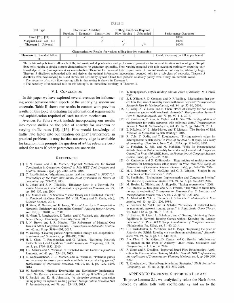
TABLE II

Toll Type Information Available Tolling Functions RequiredTopology Demands Sensitivities Flow-Varying Unbounded Performance Guarantee

Fixed [20], [21] X X X 100%Marginal-Cost [22], [23] X X† 100%Theorem 1: Universal X X‡ 100%

Characterization Results for various tolling-function constraintsTheorem 3: Bounded Affine X Good, increasing in toll upper bound

g

The relationship between allowable tolls, informational dependencies and performance guarantees for several taxation methodologies. Simplefixed tolls require a precise system characterization to guarantee optimality. Flow-varying marginal-cost tolls guarantee optimality, requiring onlyknowledge of the (homogeneous) user-sensitivities. Theorem 1’s universal tolls require none of this information, but may be arbitrarily large.Theorem 3 disallows unbounded tolls and derives the optimal information-independent bounded tolls for a sub-class of networks. Theorem 5disallows even flow-varying tolls and shows that sensitivity-agnostic fixed tolls perform relatively poorly even if they are network-aware.† The necessity of strictly flow-varying tolls in this setting is shown in Theorem 4.‡ The necessity of unbounded tolls in this setting is an immediate corollary of Theorem 3.

VII. CONCLUSION

In this paper we have explored several avenues for influenc-ing social behavior when aspects of the underlying system areuncertain. Table II shows our results in context with previousresults on this topic, illustrating the informational requirementsand sophistication required of each taxation mechanism.

Avenues for future work include incorporating our resultsinto recent studies on the price of anarchy for unknown orvarying traffic rates [15], [16]. How would knowledge oftraffic rate factor into our taxation designs? Furthermore, inpractical problems, it may be that not every edge is availablefor taxation; this prompts the question of which edges are best-suited for taxes if other parameters are uncertain.

REFERENCES

[1] P. N. Brown and J. R. Marden, “Optimal Mechanisms for RobustCoordination in Congestion Games,” in 54th IEEE Conf. Decision andControl, (Osaka, Japan), pp. 2283–2288, 2015.

[2] C. Papadimitriou, “Algorithms, games, and the internet,” in STOC ’01:Proceedings of the thirty-third annual ACM symposium on Theory ofcomputing, pp. 749–753, 2001.

[3] R. Johari and J. N. Tsitsiklis, “Efficiency Loss in a Network Re-source Allocation Game,” Mathematics of Operations Research, vol. 29,pp. 407–435, aug 2004.

[4] J. R. Marden and J. S. Shamma, “Game Theory and Distributed Control,”in Handbook of Game Theory Vol. 4 (H. Young and S. Zamir, eds.),Elsevier Science, 2014.

[5] H. Youn, M. Gastner, and H. Jeong, “Price of Anarchy in TransportationNetworks: Efficiency and Optimality Control,” Physical Review Letters,vol. 101, p. 128701, sep 2008.

[6] N. Nisan, T. Roughgarden, E. Tardos, and V. Vazirani, eds., AlgorithmicGame Theory. Cambridge University Press, 2007.

[7] P. N. Brown and J. R. Marden, “The Robustness of Marginal-CostTaxes in Affine Congestion Games,” Transactions on Automatic Control,vol. 62, no. 8, pp. 3999–4004, 2017.

[8] M. Gairing, “Covering games: Approximation through non-cooperation,”in Internet and Economics, pp. 184–195, 2009.

[9] H.-L. Chen, T. Roughgarden, and G. Valiant, “Designing NetworkProtocols for Good Equilibria,” SIAM Journal on Computing, vol. 39,no. 5, pp. 1799–1832, 2010.

[10] J. R. Marden and A. Wierman, “Distributed Welfare Games,” OperationsResearch, vol. 61, pp. 155–168, 2013.

[11] R. Gopalakrishnan, J. R. Marden, and A. Wierman, “Potential gamesare necessary to ensure pure nash equilibria in cost sharing games,”Mathematics of Operations Research, vol. 39, no. 4, pp. 1252–1296,2014.

[12] W. Sandholm, “Negative Externalities and Evolutionary Implementa-tion,” The Review of Economic Studies, vol. 72, pp. 885–915, jul 2005.

[13] F. Farokhi and K. H. Johansson, “A piecewise-constant congestiontaxing policy for repeated routing games,” Transportation Research PartB: Methodological, vol. 78, pp. 123–143, 2015.

[14] T. Roughgarden, Selfish Routing and the Price of Anarchy. MIT Press,2005.

[15] S. J. O’Hare, R. D. Connors, and D. P. Watling, “Mechanisms that gov-ern how the Price of Anarchy varies with travel demand,” TransportationResearch Part B: Methodological, vol. 84, pp. 55–80, 2016.

[16] C. Wang, X. V. Doan, and B. Chen, “Price of anarchy for non-atomiccongestion games with stochastic demands,” Transportation ResearchPart B: Methodological, vol. 70, pp. 90–111, 2014.

[17] G. Karakostas, T. Kim, A. Viglas, and H. Xia, “On the degradation ofperformance for traffic networks with oblivious users,” TransportationResearch Part B: Methodological, vol. 45, no. 2, pp. 364–371, 2011.

[18] E. Nikolova, N. E. Stier-Moses, and T. Lianeas, “The Burden of RiskAversion in Mean-Risk Selfish Routing,” 2015.

[19] R. Cole, Y. Dodis, and T. Roughgarden, “Pricing network edges forheterogeneous selfish users,” in Proc. of the 35th ACM symp. on Theoryof computing, (New York, New York, USA), pp. 521–530, 2003.

[20] L. Fleischer, K. Jain, and M. Mahdian, “Tolls for HeterogeneousSelfish Users in Multicommodity Networks and Generalized CongestionGames,” in Proc. 45th IEEE Symp. on Foundations of Computer Science,(Rome, Italy), pp. 277–285, 2004.

[21] G. Karakostas and S. Kolliopoulos, “Edge pricing of multicommoditynetworks for heterogeneous selfish users,” in Proc. 45th IEEE Symp. onFoundations of Computer Science, (Rome, Italy), pp. 268–276, 2004.

[22] M. J. Beckmann, C. B. McGuire, and C. B. Winsten, “Studies in theEconomics of Transportation,” 1955.

[23] W. Sandholm, “Evolutionary Implementation and Congestion Pricing,”The Review of Economic Studies, vol. 69, no. 3, pp. 667–689, 2002.

[24] M. Hoefer, L. Olbrich, and A. Skopalik, “Taxing subnetworks,” 2008.[25] P. J. Mackie, S. Jara-Dıaz, and A. S. Fowkes, “The value of travel time

savings in evaluation,” Transportation Research Part E: Logistics andTransportation Review, vol. 37, no. 2-3, pp. 91–106, 2001.

[26] A. Mas-Colell, “On a Theorem of Schmeidler,” Mathematical Eco-nomics, vol. 13, pp. 201–206, 1984.

[27] V. Bonifaci, M. Salek, and G. Schafer, “Efficiency of restricted tollsin non-atomic network routing games,” in Algorithmic Game Theory,vol. 6982 LNCS, pp. 302–313, 2011.

[28] U. Bhaskar, K. Ligett, L. Schulman, and C. Swamy, “Achieving TargetEquilibria in Network Routing Games without Knowing the LatencyFunctions,” in Proc. IEEE Symp. Foundations of Computer Science,(Philadelphia, PA, USA), pp. 31–40, 2014.

[29] G. Christodoulou, K. Mehlhorn, and E. Pyrga, “Improving the price ofAnarchy for Selfish Routing via coordination mechanisms,” Algorith-mica, vol. 69, no. 3, pp. 619–640, 2014.

[30] P.-a. Chen, B. De Keijzer, D. Kempe, and G. Shaefer, “Altruism andIts Impact on the Price of Anarchy,” ACM Trans. Economics andComputation, vol. 2, no. 4, 2014.

[31] R. Singh and R. Dowling, “Improved Speed-Flow Relationships: Appli-cation To Transportation Planning Models,” Seventh TRB Conference onthe Application of Transportation Planning Methods, no. 4, pp. 340–349,2002.

[32] T. Roughgarden, “Stackelberg Scheduling Strategies,” SIAM Journal onComputing, vol. 33, no. 2, pp. 332–350, 2004.

APPENDIX: PROOFS OF SUPPORTING LEMMAS

To prove Lemma 2.1, we analytically relate the Nash flowsinduced by affine tolls with coefficients κ1 and κ2 to the

10

Nash flows induced by marginal-cost tolls scaled by κ1 forsome other sensitivity distribution s′. We can then use knownanalytical techniques for scaled marginal-cost tolls to derivethe optimal κ1 and κ2. We make use of the following theorem:

Theorem 6 (Brown and Marden, [7]). For any routing prob-lem G ∈ Gp satisfying the assumptions of Theorem 3, thescaled marginal-cost taxation mechanism τ smc(κ) assigns thefollowing tolls to any edge e ∈ Gp for κ ≥ 0:

τ smce (fe) = κaefe. (35)

The unique cost-minimizing marginal-cost toll scalar is

κ∗ =1√SLSU

= arg minκ≥0

{PoA(G, τ smc(κ))} . (36)

Finally, for any G ∈ Gp, for q = SL/SU , the price of anar-chy resulting from the optimal scaled marginal-cost taxationmechanism is

PoA (G, τ smc(κ∗)) ≤ 4

3

(1−

√q(

1 +√q)2). (37)

Proof of Lemma 2.1

Let G ∈ Gp and κ1 ≥ κ2 ≥ 0.5 For user x ∈ [0, 1] withsensitivity sx ∈ [SL, SU], the cost of edge e ∈ G given flowf under affine tolls is given by

Jex(f) = (1 + κ1sx)aefe + (1 + κ2sx)be.

Note that we may scale Jex(f) by any edge-independent factorwithout changing the underlying preferences of agent x. Thus,without loss of generality, we may write

Jex(f) =1 + κ1sx1 + κ2sx

aefe + be. (38)

Now, define sensitivity distribution s′ by the following: forany x ∈ [0, 1], s′x satisfies

s′x =sx(κ1 − κ2)

κ1(1 + κ2sx). (39)

By a series of algebraic manipulations, we may combine (38)and (39) to obtain

Jex(f) = (1 + κ1s′x) aefe + be, (40)

which is simply the cost resulting from scaled marginal-costtolls (35). Thus, for any sensitivity distribution s, we maymodel a Nash flow resulting from affine tolls with coefficientsκ1 and κ2 as a Nash flow for sensitivity distribution s′

resulting from scaled marginal-cost tolls with κ = κ1.Thus, by Theorem 6, assuming first that κmax is sufficiently

high, our optimal choice of κ1 is that which satisfies

κ1 =1√S′LS

′U

, (41)

where S′L and S′U are computed according to (39).Combining (39) and (41) yields the following character-

ization of the optimal κ2 with respect to κ1, for κmax ≥(SLSU)

−1/2:

5Here, the requirement that κ1 ≥ κ2 is without loss of generality; lateranalysis shows that κ2 > κ1 would always result in a Nash flow with highercongestion than the un-tolled case.

κ2 =κ21SLSU − 1

SL + SU + 2κ1SLSU. (42)

Evaluating (37) at q = S′L/S′U verifies the second part

of (23) as the correct expression for PoA(G, τA(κ∗1, κ

∗2))

when κmax is large.Consider the case when κmax < (SLSU)

−1/2. Now, (42)would prescribe a negative value for κ2, so the optimal choiceis to let κ2 saturate at 0. Now, we are precisely applyingscaled marginal-cost tolls with κ = κ1, so we apply the factshown in Lemma 1.2 of [7] that on this class of networks, ifκ ≤ (SLSU)

−1/2, the worst-case total latency of a Nash flowalways occurs for the extreme low-sensitivity homogeneoussensitivity distribution given by sx ≡ SL for all x ∈ [0, 1].

Equation (35) in [7] gives the total latency of a Nash flowfor a homogeneous population with sensitivity SL as

Lnf(G,SL, κ) = LR −κSL

(1 + κSL)2 Θ, (44)

where LR and Θ are positive constants depending only onG, satisfying Θ ≤ LR. It is easy to verify that the aboveexpression is minimized on a subset of

[0, (SLSU)

−1/2]

bymaximizing κ, and using the fact that Θ ≤ LR, we may verifythat the price of anarchy for κmax < (SLSU)

−1/2 is given bythe first part of (23), completing the proof of Lemma 2.1.

Proof of Lemma 2.2

Here, we derive properties of any taxation mechanism thatoutperforms τA(κ∗1, κ

∗2). We define the set of routing problems

G0 as follows: G ∈ G0 is a parallel network consisting of twoedges, with `1(f1) = cf1 and `2(f2) = c.

Let G ∈ G0. For any c, the optimal flow on G is (f∗1 , f∗2 ) =

(1/2, 1/2) and the optimal total latency is L∗(G) = 3c/4, butthe un-tolled Nash flow has a total latency of Lnf(G, s, ∅) = c,so the un-tolled price of anarchy is 4/3. It is straightforwardto show furthermore that if SU > SL ≥ 0, for any κmax > 0,this network constitutes a worst-case example and the priceof anarchy bound of this particular network is tight; i.e., itequals the expression given in (23): PoA

(G, τA(κ∗1, κ

∗2))

=supG∈Gp PoA

(G, τA(κ∗1, κ

∗2)). Thus, if our hypothetical τ∗

outperforms τA in general, it must specifically outperform τA

on any network G ∈ G0, or

PoA (G, τ∗) < PoA(G, τA(κ∗1, κ

∗2)). (45)

Now, we investigate the performance of the hypotheticaltolling mechanism τ∗ on networks in G0. Given a networkG ∈ G0, τ∗ assigns edge tolling functions τ∗1 (f1) and τ∗2 (f2).Recall that since τ∗ is network-agnostic, there is some functionτ∗ (f ; a, b) such that an edge e ∈ E with latency function`e(fe) = aefe + be is assigned tolling function τ∗(fe; ae, be).By analyzing networks in G0, we can deduce properties ofthe function with the 2nd and 3rd arguments set to 0, sinceτ∗1 (f1) = τ∗(f1; c, 0) and τ∗2 (f2) = τ∗(f2; 0, c).

Now we show that τ∗ must assign higher tolls thanτA(κ∗1, κ

∗2). Let SU > SL. By design, the worst-case Nash

flows resulting from τA(κ∗1, κ∗2) occur for homogeneous pop-

ulations with s = SL and s = SU. Since any network G ∈ G0has only 2 links, we can characterize a Nash flow simply by

11

κ1(U) = min

Ta , 2TSLSU − (SL + SU)a+√

((SL + SU) a+ 2TSLSU)2

+ 4bSLSU

(2a+ b+ T (SL + SU)

)2SLSU

(2a+ b

) (43)

Fig. 7. Closed-form expression for κ1(U) used in Theorem 3. Note that it is a continuous, unbounded, strictly increasing function of T .

the flow on edge 1; accordingly, let fL(c) denote the flow asa function of c on edge 1 in the Nash flow resulting fromsensitivity distribution s = SL, and fH(c) the correspondingedge 1 flow for s = SU. These flows are the solutions to thefollowing equations:

cfL(c) (1 + κ∗1SL) = c (1 + κ∗2SL) , (46)cfH(c) (1 + κ∗1SU) = c (1 + κ∗2SU) . (47)

Summing (46) and (47) yields

κ∗1 (fL(c)− fH(c)) =fH(c)

SU− fL(c)

SL+

1

SL− 1

SU. (48)

It is always true that fH(c) < fL(c). By design, L(fL(c)) =L(fH(c)). Note that L is simply a concave-up parabola in theflow on edge 1.

Now, let f∗L(c) and f∗H(c) be defined as the Nash flowsresulting from τ∗ for a given value of c; i.e., the solutions to

cf∗L(c) + τ∗1 (f∗L(c))SL = c+ τ∗2 (1− f∗L(c))SL, (49)cf∗H(c) + τ∗1 (f∗H(c))SU = c+ τ∗2 (1− f∗H(c))SU. (50)

Since τ∗ guarantees better performance than τA(κ∗1, κ∗2), it

must do so in particular for these homogeneous sensitivitydistributions s = SL and s = SU. Since L is a parabola, thismeans that for any c, fH(c) < f∗H(c) < f∗L(c) < fL(c).

Define the nondecreasing function ∆∗(f) = τ∗2 (f)−τ∗1 (1−f) (which is implicitly also a function of c), so equations (49)and (50) can be combined and rearranged to show

∆∗(f∗L(c))−∆∗(f∗H(c)) > c

[fH(c)

SU− fL(c)

SL+

1

SL− 1

SU

]= κ∗1c (fL(c)− fH(c)) (51)

The above inequality can be further loosened by replacingf∗L(c) with fL(c) and f∗H(c) with fH(c), and substitutingfrom (48) and rearranging, we finally obtain

∆∗(fL(c))−∆∗(fH(c))

fL(c)− fH(c)> κ∗1c. (52)

Since this must be true for any c > 0, the average slope of∆∗(f) must be greater than κ∗1c for all f > 0. Since τ∗2 (f) ≥ 0this implies that τ∗1 (f) > κ∗1cf for all f > 0, or that

τ∗(f ; a, 0) > τA(f ; a, 0) (53)

for all positive f and a.Now consider the following rearrangement of (50):

τ∗2 (1− f∗H(c)) = [cf∗H(c) + τ∗1 (f∗H(c))− cSU] · 1

SU

> c [(1 + κ∗1SU) fH(c)− 1] · 1

SU

= κ∗2cSU = τA2 (f). (54)

This implies that τ∗2 (f) > κ∗2c for all f > 0, or that

τ∗(f ; 0, b) > τA(f ; 0, b) (55)

for all positive f and b.Finally, note that the additivity assumption of Definition 2

implies that τ∗(f ; a, b) is additive in its second and thirdarguments. That is, we may add inequalities (53) and (55)to conclude that for all nonnegative f , a, and b, it is true that

τ∗(f ; a, b) > κ∗1af + κ∗2b, (56)

or that a necessary condition for supG∈Gp PoA(G, τ∗) <supG∈Gp PoA(G, τA) is that τ∗ must charge higher tolls onevery edge in every network.

Proof of Lemma 5.1

We first derive a simple expression for a Nash flow for ahomogeneous population as a linear function of the tolls τ .Note that in the context of fixed tolls, Nash flows are uniquein cost: for a given routing game, every Nash flow exhibitsthe same cost on all edges [19].

Claim 5.1.1. A Nash flow on G ∈ G for sensitivity s ∈ S1and fixed tolls τ ∈ Rn that has positive traffic on all links canbe described by the following linear function:

f ft(G, s, τ) = R+H(b+ sτ), (57)

where R ∈ Rn and H ∈ Rn×n are constant matricesdepending only on G. The total latency of this flow is givenby the following convex quadratic in τ :

Lft(G, s, τ) = LR + sτTHT (2AH + I)b+ s2τTHTAHτ.(58)

Proof. Since all users share the same sensitivity, all links haveequal cost to all agents in a Nash flow, so when all networkedges have positive flow, for any ei, ej ∈ E,

aifi + bi + sτi = ajfj + bj + sτj .

Similar to the approach in the proof of Lemma 1.2 in [7], aNash flow f ft(G, s, τ) is a solution f to the linear systema1 −a2 · · · 00 a2 · · · 0... 0

. . ....

1 1 · · · 1

︸ ︷︷ ︸

P

f =

0...01

︸︷︷︸r

+

−1 1 · · · 00 −1 · · · 0... 0

. . ....

0 0 · · · 0

︸ ︷︷ ︸

X

(b+ sτ).

(59)P is invertible, so letting H = P−1X and R = P−1r, a Nashflow is given by the linear equation (57).

The following observations will be helpful to our proof:

12

Observation 5.1. The matrices H and R possess the followingproperties for any G ∈ G:

1THb = 0T, (60)

1TR = 1, (61)AR ∈ sp {1} , (62)

bTHTAHb = −MT b. (63)

Finally, every column of (AH + I) is in sp{1}.

These facts follow algebraically from the fact that by defi-nition, f ft(G, s, τ) satisfies (59). Subsutiting (57) into (1) andsimplifying using the facts in Observation 5.1 yields (58).

Next, we establish a necessary condition for a set of fixedtolls to be optimal in the sense of (33).

Claim 5.1.2. Fixed tolls τ∗ satisfying (33) must also satisfy

H

(τ∗ +

b

SL + SU

)= 0. (64)

Proof. By (58) the total latency due to fixed tolls is a concaveparabola in s, so for any τ , the maximum total latency on[SL, SU] occurs at either SL or SU. Since Lft(G, s, τ) iscontinuous and convex in τ , this means that τ∗ must satisfy

Lft(G,SL, τ∗) = Lft(G,SU, τ

∗). (65)

Thus, for any optimal fixed tolls τ∗, Lft(G, s, τ∗) is a parabolacentered at s = SL+SU

2 :

argmins∈[SL,SU]

Lft(G, s, τ∗) = (SL + SU)/2. (66)

Our goal is to find the parabola with minimum as in (66)which minimizes the values in (65).

Equation (58) implies that for all τ, τ ′ ∈ Rn, Lft(G, 0, τ) =Lft(G, 0, τ ′); that is, the s = 0 endpoint of the parabolahas the same value for all tolls. Thus, for τ satisfy-ing (66), Lft(G,SL, τ

∗) < Lft(G,SL, τ) if and only ifLft(G, SL+SU

2 , τ∗)< Lft

(G, SL+SU

2 , τ).

By concavity, any tolls which result in globally optimalrouting for s = SL+SU

2 will also be optimal in the senseof (33). It is easily verified that for a known homogeneoussensitivity s, any tolls τ which satisfy

H (τ + b/(2s)) = 0 (67)

result in globally optimal routing. The proof of this is obtainedby substituting (67) into the gradient (with respect to τ ) ofLft(G, s, τ) and applying the facts from Observation 5.1.

Therefore, any τ which satisfies (67) with s = SL+SU

2 willbe uncertainty-optimal. That is, τ∗ satisfies (64).

Evaluating (57) with tolls satisfying (64) yields an expres-sion for a Nash flow induced by τ∗ as a function of s:

f ft(G, s, τ∗) = R+Hb (SL + SU − s) / (SL + SU) , (68)

implying that (R+Hb) specifies an un-tolled Nash flow. Forparallel networks, it is easy to show that every element of Ris non-negative; thus, since α ,

(SL+SU−sSL+SU

)∈ [0, 1], it must

be that (R+Hbα) represents a feasible flow.

There are two possible worst-case flows using fixed toll τ∗:one when the sensitivity is SU, the other when the sensitivityis SL. In terms of (68), we write these flows as:

f ft− = f ft(G,SL, τ∗) = R+Hb (SU/(SL + SU)) . (69)

f ft+ = f ft(G,SU, τ∗) = R+Hb (SL/(SL + SU)) . (70)

Next we show that f ft− and f ft+ , the worst-case flows foroptimal fixed tolls, are actually exactly equal to worst-caseflows achievable with scaled marginal-cost tolls (35) witha particular scalar. The machinery of Claim 5.1.1 describesthe Nash flows f smc(G, s, κ) resulting from homogeneoussensitivity s and marginal-cost tolls scaled by κ > 0:

f smc(G, s, κ) = R+Hb/ (1 + sκ) . (71)

The derivation of this is straightforward; it is detailed in [7].The worst worst-case flows occur when the sensitivity of

the population has been grossly over- or under-estimated; forexample, if a population with sensitivity SU is using a networkwith κ = 1/SL (and vice-versa). There are two such flows:

f smc− = R+

Hb

1 + SL/SUand f smc

+ = R+Hb

1 + SU/SL.

Comparing the above to (69) and (70), we see that f smc− = f ft−

and f smc+ = f ft+ . Thus, since

f ft(G,SL, τ∗) = f smc(G,SL, 1/SU),

f ft(G,SU, τ∗) = f smc(G,SU, 1/SL),

it must be true that (re-writing now in terms of affine tolls)

Lnf(G,SL, τ∗) = Lnf(G,SL, τ

A(1/SU, 0)), (72)

Lnf(G,SU, τ∗) = Lnf(G,SU, τ

A(1/SL, 0)). (73)

By design, (72) equals (73), so we have that

maxs∈[SL,SU]

Lnf(G, s, τA(1/SU, 0)

)= maxs∈[SL,SU]

Lnf (G, s, τ∗) .

Philip N. Brown is a PhD candidate in the Department of Electrical andComputer Engineering at the University of California, Santa Barbara. Philipreceived the Bachelor of Science in Electrical Engineering in 2007 fromGeorgia Tech, after which he spent several years designing control systemsand process technology for the biodiesel industry. He received the Master ofScience in Electrical Engineering in 2015 from the University of Colorado atBoulder under the supervision of Jason R. Marden, where he was a recipientof the University of Colorado Chancellor’s Fellowship.

Jason R. Marden is an Assistant Professor in the Department of Electricaland Computer Engineering at the University of California, Santa Barbara.Jason received the Bachelor of Science in Mechanical Engineering in 2001from UCLA, and the PhD in Mechanical Engineering in 2007, also fromUCLA, under the supervision of Jeff S. Shamma, where he was awardedthe Outstanding Graduating PhD Student in Mechanical Engineering. Aftergraduating from UCLA, he served as a junior fellow in the Social andInformation Sciences Laboratory at the California Institute of Technologyuntil 2010, and then as an Assistant Professor at the University of Coloradountil 2015. Jason is a recipient of an ONR Young Investigator Award (2015),NSF Career Award (2014), AFOSR Young Investigator Award (2012), SIAMCST Best Sicon Paper Award (2015), and the American Automatic ControlCouncil Donald P. Eckman Award (2012). Jason’s research interests focus ongame theoretic methods for the control of distributed multiagent systems.