Federal Reserve Bank of Dallas Globalization and Monetary Policy Institute

Working Paper No. 272 http://www.dallasfed.org/assets/documents/institute/wpapers/2016/0272.pdf

Optimal Monetary Policy in Open Economies Revisited*

Ippei Fujiwara

Keio University and ANU

Jiao Wang Australian National University

May 2016

Abstract This paper revisits optimal monetary policy in open economies, in particular, focusing on the noncooperative policy game under local currency pricing in a two-country dynamic stochastic general equilibrium model. We first derive the quadratic loss functions which noncooperative policy makers aim to minimize. Then, we show that noncooperative policy makers face extra trade-offs regarding stabilizing the real marginal costs induced by deviations from the law of one price under local currency pricing. As a result of the increased number of stabilizing objectives, welfare gains from cooperation emerge even when two countries face only technology shocks, which usually leads to equivalence between cooperation and noncooperation. Still, gains from cooperation are not large, implying that frictions other than nominal rigidities are necessary to strongly recommend cooperation as an important policy framework to increase global welfare. JEL codes: E52, F41, F42

* Ippei Fujiwara, Keio University A2-15-45 Mita, Minato-ku, Tokyo 108-8345 Japan. ippei.fujiwara@keio.jp. Jiao Wang, Australian National University, Canberra ACT 0200 Australia. jiao.wang@anu.edu.au. We have benefited from discussions with Kosuke Aoki, Pierpaolo Benigno, Richard Dennis, Mick Devereux, Charles Engel, Jinill Kim, Warwick McKibbin and seminar participants at the Australian National University and the University of Melbourne. Fujiwara is grateful for financial support from JSPS KAKENHI Grant-in-Aid for Scientific Research (A) Grant Number 15H01939. The views in this paper are those of the authors and do not necessarily reflect the views of the Federal Reserve Bank of Dallas or the Federal Reserve System.

1 IntroductionIn a world of integrated trade in goods and assets, sovereign nations become moreand more interdependent. The prolonged recession after the Global Financial Crisisagain reminds policy makers in major economies of the depth and scope of such inter-relations. Understanding the nature of cross-country spillovers of shocks and policyimpacts comes back to center stage in policy discussions. Should central banks co-operate in order to internalize the possible externality from policy reactions? Is thereany gain from such cooperation? And if so, how large might it be?

The desirability of policy cooperation, namely whether there exist gains from co-operation, has been one of the central issues in macroeconomics. The root of the dis-cussion can be traced way back to Hume (1752), who first noticed possible policyspillovers among countries. Since then, there have been vast studies investigatingthe nature of policy games in open economies. Recently, many have studied optimalmonetary policy in open economies using the microfounded, open-economy sticky-price models based on the so-called New Open Economy Macroeconomics (hereafter,NOEM) initiated by Obstfeld and Rogoff (1995) and Svensson and van Wijnbergen(1989). Contrary to the traditional studies using the Mundell-Fleming model, cor-rect welfare can be computed with the NOEM models. Thus, comparison of differentpolicies becomes possible without resort to ad hoc criteria.

As will be discussed in detail in the next subsection, optimal monetary policy inopen economies has been investigated under many different settings in the NOEM,such as under cooperation or noncooperation, producer currency pricing (hereafter,PCP) or local currency pricing (hereafter, LCP), and with or without home bias. Con-sequently, our understanding of how monetary policy should be conducted in an in-terconnected world is deepened. There is, however, one last missing piece, which hasnot yet been analyzed in a theoretical dynamic stochastic general equilibrium (here-after, DSGE) model. That is, how the optimal noncooperative monetary policy underLCP should be conducted, or whether there is any gain from cooperation under LCP.These are the questions to which we aim to give answers in this paper.

For this purpose, we first solve the equilibrium conditions under monopolisticcompetition and sticky prices in a two-country model. Also, the Ramsey (determinis-tic) steady states under both cooperative and noncooperative regimes are computed.In both schemes, the deterministic steady state turns out to be identical to that underthe flexible-price equilibrium.1 Thus, the exact welfare comparison between cooper-ation and noncooperation becomes possible. Then, we approximate welfare aroundthis deterministic steady state up to the second order. In a noncooperative regime,

1In addition, this steady state is at efficient levels since the optimal sales subsidy, which is identicalregardless of cooperation and noncooperation, eliminates the steady state distortion stemming fromsuboptimally low output under monopolistic competition. Early literature with the linear-quadraticoptimal monetary policy problems such as Rotemberg and Woodford (1997) or Woodford (2003) as-sume such a subsidy to obtain the correct second-order approximated welfare. Benigno and Woodford(2005) propose a method to compute the correct second-order welfare measure when the steady stateis distorted.

2

even if the steady state is efficient thanks to the optimal subsidy, linear terms can-not be eliminated. Following Sutherland (2002), Benigno and Woodford (2005) andBenigno and Benigno (2006), we take a second-order approximation to the structuralequations to substitute out the linear terms by only second-order terms. Correct wel-fare metrics up to the second-order approximation are thus obtained.

Our loss functions show that noncooperative policy makers naturally aim to sta-bilize variables whose fluctuations are to be minimized by cooperative policy makersas analyzed in Engel (2011), including output, producer price index (hereafter, PPI)inflation rates, import price inflation rates, and deviations from the law of one price.2In addition, they also seek to stabilize fluctuations in the real marginal costs that firmsface when setting prices in both domestic and export markets. These additional ob-jectives are unique to the noncooperative game and therefore the sources for potentialgains from cooperation, which are absent in the previous studies on optimal monetarypolicy in open economies.3

Then, in order to clarify the nature of optimal monetary policy in open economies,we compare impulse responses under optimal monetary policies among three cases:(1) PCP; (2) cooperative regime and LCP; (3) noncooperative regime and LCP. Notethat in our setting with only technology shocks, optimal cooperative as well as non-cooperative policies result in identical allocations and prices under PCP.4

Fluctuations in consumer price index (hereafter, CPI) inflation rates become smallerunder LCP than under PCP. This is because the violation of the law of one price in-duces inefficient price dispersions within producer as well as export prices, as em-phasized by Engel (2011). As a result, the ‘inward-looking’ policy that focuses onstabilization of PPI inflation rates is no more optimal under LCP. In addition, underLCP, noncooperative policy makers stabilize CPI inflation rates more than cooperativecentral banks do. This larger stabilization motive arises from the unique objectives inthe loss functions under noncooperation. Inability to cooperate constrains the dy-namics toward more efficient outcomes. Reactions of domestic output to a domestictechnology shock become smaller under noncooperation. Without any frictions, theglobal welfare increases when the production of the country with favorable efficiencyshocks increases. This difference in the responses of output creates room for coopera-tive policies to improve global welfare.

We also compute the welfare gain from cooperation under LCP by solving the non-linear Ramsey problem. Welfare gains from cooperation become largest with log util-ity even though both countries become insular in structural equations under PCP. Still,welfare gains computed from nonlinear Ramsey problems are not sizable with onlytechnology shocks. Within the reasonable range of parameter calibration, the wel-

2Note that last terms are not considered under PCP, since the law of one price holds.3Technically, these additional objectives arise from the linear terms in the second-order approxi-

mated welfare, that are eventually substituted by second-order approximated aggregate supply condi-tions.

4Note that our model assumes a Cobb-Douglas aggregator for domestic and foreign goods. Forthe cases where cooperative and noncooperative policies produce different outcomes, see Benigno andBenigno (2003).

3

fare cost stemming from the inability to cooperate can only be, at most, 0.04 per centin consumption units, in response to one standard deviation of technology shocks.Corsetti (2008) remarks that in early leading studies, the quantitative assessment ofthe welfare gains from cooperation is found far from sufficient to be in favor of coop-eration, and whether it still holds in richer models is a critical research question. Ourpaper finds that given only price rigidities,sizable welfare gains may not arise fromcooperation.

1.1 Literature ReviewLet us first classify the previous studies on optimal monetary policy in open economiesby three dimensions.5 The first dimension regards the assumption on nominal rigidi-ties, that is, either the one-period ahead price setting or the staggered price setting ala Calvo (1983).6 In early studies using the NOEM framework, nominal rigidities areintroduced as the one-period ahead price setting. With money supply as the controlvariable of monetary policy, analytical solutions can be obtained. Thus, no approxi-mation is necessary for optimal policy analysis. With more relevance to the price set-ting behavior and monetary policy in practice, the staggered price contract togetherwith nominal interest rates controlled by the central bank becomes the major assump-tion about nominal frictions, in particular after Clarida, Galı, and Gertler (2002) in theopen-economy context.7 In contrast to the one-period ahead price setting, optimalmonetary policy is analyzed in a linear-quadratic framework following Rotembergand Woodford (1997), Woodford (2003) and Benigno and Woodford (2005). Centralbanks maximize the correctly approximated social welfare up to the second order sub-ject to the linearly approximated structural equations. The second dimension is aboutexport price setting, namely PCP or LCP.8 In the former, export prices fully reflect ex-change rate fluctuations, while not at all in the latter. The third dimension is whethermonetary policy in open economies is conducted in a cooperative or noncooperativemanner.

Table 1 offers a taxonomy of previous studies on optimal monetary policy in openeconomies. Regarded as the beginning of the NOEM framework for monetary pol-icy analysis in open economies, Obstfeld and Rogoff (1995) develop a micro-foundedtwo-country model with PCP and a one-period in advance price setting rule to ana-

5Corsetti, Dedola, and Leduc (2010) offer a comprehensive survey of optimal monetary policy inopen economies including other aspects such as financial market imperfections.

6Rotemberg (1982) proposes a different type of price stickiness due to a staggered cost adjustmentprocess.

7According to the Calvo rule, firms reset prices in a forward-looking rational expectation manner.This raises the question of how to affect and/or manage the private sector’s rational expectation formonetary policy practice. Related theoretical discussions include conducting monetary policy undercommitment versus under discretion, delegation problem, credibility of cooperation, targeting rulesversus instrument rules, etc.. Investigation of these issues are beyond the scope of this paper. As anincomplete list, see, for example, Persson and Tabellini (1995), Benigno (2002), Bilbiie (2002), Jensen(2002), Woodford (2003) and Svensson (2002, 2003, 2004).

8Corsetti and Pesenti (2005b) briefly analyze a third and less used pricing behavior: Dollar-pricing.

4

lyze the dynamics of exchange rates and other variables in response to money supplyshocks. Their investigation of the (log-linearized) global welfare appraises the first-order welfare effect of monetary expansion on raising global demand and world out-put. It also suggests that the conventional Mundell-Fleming paradigm may overstatethe importance of the beggar-thy-neighbor effects that a currency-depreciating countryinflicts on trading partners since the induced terms-of-trade and current-account ef-fects are only of second-order welfare importance. Corsetti and Pesenti (2001) extendthe model of Obstfeld and Rogoff (1995) to highlight the international dimension ofdistortions stemming from a country’s monopoly power on its terms of trade by as-suming different elasticities of substitution within and across goods categories.9 Theykeep the assumptions of PCP, one-period ahead price resetting rule and money supplyshocks but focus on national welfares. A domestic monetary expansion can be eitherbeggar-thy-neighbor or beggar-thyself depending on the elasticity of substitution, givingrise to national policy makers’ incentives to manipulate the terms of trade in favorof their own welfare. Obstfeld and Rogoff (2002) assume the one-period ahead rulefor nominal wage setting (prices for goods are flexible) and the existence of the non-tradable sector for their examination of international cooperation under PCP. Utilityof each country is expressed in terms of covariances of logs of endogenous variables,and monetary rules are assumed as explicit (log-linear) functions of exogenous pro-ductivity shocks in a stochastic environment.10 When nominal stickiness has littleinteraction with real distortions, welfare gains from cooperation (in percentage out-put) are relatively small.11

Devereux and Engel (2003) assume LCP and both strategic games in a two-countrymodel while keeping the price setting in the period-by-period basis.12 They deriveand compare optimal monetary rules (as log-linear functions of productivity and ve-locity shocks) to examine the desirability of flexible exchange rates as advocated inFriedman (1953). The flexible exchange rate regime is no longer optimal under LCP.Distortions stemming from the violation of the law of one price should be correctedby restricting the fluctuations of nominal exchange rates. Thus, optimal policy underLCP fully stabilizes fluctuations in exchange rates in both games. Corsetti and Pe-senti (2005a) propose a unifying approach to model the exchange rate pass-throughin which PCP and LCP are two extreme cases of the parameterization.13 No welfaregains from cooperation are found under either complete or no exchange rate pass-through. In general cases with partial exchange rate pass-through they argue that acountry can do better than ‘keeping one’s house in order’ but whether the gains are

9For a detailed discussion on this issue, see Tille (2001).10Productivity shocks, along with cost-push shocks, become the main sources of exogenous distur-

bances that optimal monetary policy responds to in later studies.11Note that Obstfeld and Rogoff (2002) define the cooperation gain as the gain from deviating from

flex-wage equilibrium to cooperative equilibrium. Noncooperative equilibrium lies between the flex-wage and cooperative policy responses and thus the estimation is an upper bound on the gains frommoving from noncooperation to cooperation.

12Much empirical evidence points to the possibility of LCP, see, for example, Engel (1999), Engel andRogers (2001), Parsley and Wei (2001), and Atkeson and Burstein (2008).

13Corsetti and Pesenti (2005a) also offer insights from the staggered price setting.

5

sizable is left for future studies with more realistic model settings.Clarida, Galı, and Gertler (2002), Benigno and Benigno (2003, 2006) all assume

the staggered price adjustment rule a la Calvo (1983) and obtain quadratic loss func-tions under cooperation as well as noncooperation for their respective optimal policyanalysis under PCP.14 By contrast, Clarida, Galı, and Gertler (2002) choose output aspolicy variables under noncooperative regime and set the first derivative of nationalutility function to zero by assuming an appropriate subsidy to eliminate the linearterms in the second-order approximation of the utility function. As a result, Ramseysteady states become different between cooperation and noncooperation. Benignoand Benigno (2003) set up a ratio of the notional price over the average actual price asnoncooperative policy instruments, and obtain a zero first derivative of the nationalutility function from households’ price setting condition as monopolists selling goodsto achieve the elimination of the linear terms. The quadratic loss function under non-cooperation can be derived since price stability turns out to be optimal monetary pol-icy. Benigno and Benigno (2006) choose PPI inflation rates for their noncooperativegames and make use of second-order approximations of some of the structural equa-tions to substitute out those linear terms following Sutherland (2002) and Benignoand Woodford (2005). Besides the methodological differences, these three studies alsotake on different focuses on the implications of optimal policy analysis. Specifically,Clarida, Galı, and Gertler (2002) appraise the potential gains from cooperation arisingfrom internalizing the terms-of-trade externalities, in the context of (inefficient) cost-push shocks and discretionary optimal policy. Benigno and Benigno (2003) explorethe theoretical conditions under which flexible-price allocations are optimal, and co-operative and noncooperative allocations coincide under PCP. Finally, Benigno andBenigno (2006) show how to design simple rules for noncooperative policy makersto achieve cooperative allocations in the linear-quadratic framework with technologyshocks, markup shocks and government spending shocks.

Engel (2011) incorporates the staggered price setting rule for optimal monetaryanalysis under LCP and the cooperative regime. Home bias in consumption prefer-ences is also assumed.15 With home bias, central banks face the trade-off between thecosts of currency misalignment and stabilization of asymmetric output fluctuations.The derived quadratic global loss function highlights international relative price mis-alignments stemming from the violation of the law of one price under LCP. Thus,optimal cooperative policy under LCP should trade off these misalignments with in-flation and output goals, and should target CPI inflation rates rather than just PPIinflation rates. Our paper is an extension from Engel (2011) to the noncooperativegame, providing the final block of the class of the NOEM literature as summarized in

14Benigno and Benigno (2003) also assume a one-period ahead price setting rule for policies undercommitment and the Calvo rule for policies under discretion.

15Faia and Monacelli (2008) and Duarte and Obstfeld (2008) also consider different consumptionpreferences for a similar purpose.

6

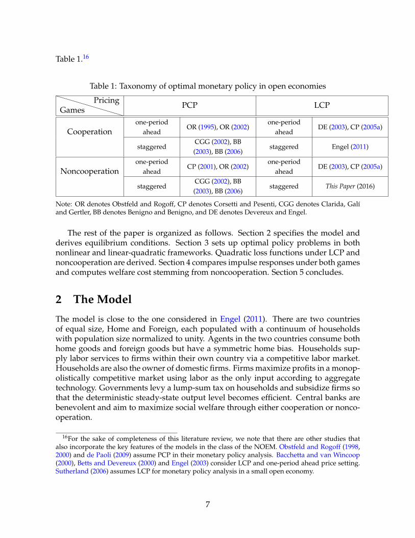
Table 1.16

Table 1: Taxonomy of optimal monetary policy in open economies

GamesPricing PCP LCP

Cooperationone-period

aheadOR (1995), OR (2002)

one-periodahead

DE (2003), CP (2005a)

staggeredCGG (2002), BB(2003), BB (2006)

staggered Engel (2011)

Noncooperationone-period

aheadCP (2001), OR (2002)

one-periodahead

DE (2003), CP (2005a)

staggeredCGG (2002), BB(2003), BB (2006)

staggered This Paper (2016)

Note: OR denotes Obstfeld and Rogoff, CP denotes Corsetti and Pesenti, CGG denotes Clarida, Galıand Gertler, BB denotes Benigno and Benigno, and DE denotes Devereux and Engel.

The rest of the paper is organized as follows. Section 2 specifies the model andderives equilibrium conditions. Section 3 sets up optimal policy problems in bothnonlinear and linear-quadratic frameworks. Quadratic loss functions under LCP andnoncooperation are derived. Section 4 compares impulse responses under both gamesand computes welfare cost stemming from noncooperation. Section 5 concludes.

2 The ModelThe model is close to the one considered in Engel (2011). There are two countriesof equal size, Home and Foreign, each populated with a continuum of householdswith population size normalized to unity. Agents in the two countries consume bothhome goods and foreign goods but have a symmetric home bias. Households sup-ply labor services to firms within their own country via a competitive labor market.Households are also the owner of domestic firms. Firms maximize profits in a monop-olistically competitive market using labor as the only input according to aggregatetechnology. Governments levy a lump-sum tax on households and subsidize firms sothat the deterministic steady-state output level becomes efficient. Central banks arebenevolent and aim to maximize social welfare through either cooperation or nonco-operation.

16For the sake of completeness of this literature review, we note that there are other studies thatalso incorporate the key features of the models in the class of the NOEM. Obstfeld and Rogoff (1998,2000) and de Paoli (2009) assume PCP in their monetary policy analysis. Bacchetta and van Wincoop(2000), Betts and Devereux (2000) and Engel (2003) consider LCP and one-period ahead price setting.Sutherland (2006) assumes LCP for monetary policy analysis in a small open economy.

7

2.1 HouseholdsA representative household in the home country maximizes welfare:

WH,t0 ⌘ Et0

•

Ât=t0

bt�t0 [u (Ct)� v (ht)] (2.1)

subject to the budget constraint:

Et [mt,t+1At+1] + Bt+1 + PtCt At + (1 + it�1) Bt + Wtht + Pt + Tt,

for t � t0, where the consumption aggregator Ct, the aggregate consumption of locallyproduced goods CH,t, and the aggregate consumption of imported goods CF,t is givenby

Ct = Cn2H,tC

1� n2

F,t , (2.2)

CH,t =

"1

0CH,t (j)1� 1

# dj

# ##�1

, (2.3)

CF,t =

"1

0CF,t (j⇤)1� 1

# dj⇤# #

#�1

, (2.4)

respectively. u (.) is the period utility function, increasing and concave in consump-tion. v (.) is the period disutility function, increasing and convex in labor ht (mea-sured by working hours). Wt denotes the nominal wage. At+1 denotes the holdingsof the state contingent (Arrow) securities at the end of period t denominated in thedomestic currency, which equates the marginal rates of substitutions of two countrieseven ex post. mt,t+1 denotes the price of the Arrow securities in period t which givesan unitary return in period t + 1. Bt is the amount of one-period risk-free nominalbonds held at the beginning of period t with net rate of return it�1. Pt represents thedividend from the ownership of firms. Tt represents the lump-sum tax levied by thegovernment. b is the discount factor. e denotes the elasticity of substitution amongdifferentiated varieties within each country. n 2 [0, 2] determines the (symmetric)home bias. When n is larger (smaller) than unity, consumer preference exhibits home(foreign) bias. There is no home bias when n equals unity. CH,t (j) and CF,t (j⇤) de-note the home representative household’s consumption of the goods produced by thehome firm j and the foreign firm j⇤, respectively. Note that Lagrange multipliers onthe constraints in equations (2.2) to (2.4) represent CPI Pt, PPI PH,t, and the importprice index PF,t. A representative household in the foreign country solves a similaroptimization problem on the welfare:

WF,t0 ⌘ Et0

•

Ât=t0

bt�t0 [u (C⇤t )� v (h⇤t )] . (2.5)

8

2.2 FirmsFirm j in the home country sets prices in a monopolistically competitive market tomaximize the present discounted value of profits:

Et0

•

Ât=t0

qt�t0mt0,tPt (j) ,

where

Pt (j) = (1 + t) PH,t(j)CH,t(j) + (1 + t) StP⇤H,t(j)C⇤

H,t(j)� Wtht (j)

subject to the production function:

Yt (j) = exp (zt) ht (j) , (2.6)

and the resource constraint:

Yt (j) = CH,t(j) + C⇤H,t(j). (2.7)

St denotes the nominal exchange rate of the foreign currency in units of the home cur-rency. t represents the government subsidy rate. Firm j produces Yt (j) of the productby hiring ht (j) of labor service from the domestic households according to aggregateproduction technology exp (zt), where zt follows an AR(1) exogenous process. Firmsset their optimal prices in a staggered manner a la Calvo (1983) rule. Each time, onlywith probability 1� q, can they re-optimize their prices. Note that the Lagrange multi-plier on a constraint where the production function in equation (2.6) and the resourceconstraint in equation (2.7) are combined represents nominal marginal costs:

NMCt =Wt

exp (zt).

There is no firm specificity in marginal costs.Regarding the export price, there are two types of price setting. Under PCP, firms

fully reflect changes in exchange rates in export prices. Thus, the law of one priceholds:

PH,t(j) = StP⇤H,t(j).

On the other hand, under LCP, firms faces the same Calvo (1983) friction even whensetting export prices. As a result, firm j reoptimizes both PH,t(j) and P⇤

H,t(j) in orderto maximize profits.17

Firm j⇤ in the foreign country solves a similar profit maximization problem.

17We do not consider interim cases as in Monacelli (2005).

9

2.3 Governments and Central BanksThe government in each country collects a lump sum tax from households and subsi-dizes firms to eliminate steady state distortions stemming from monopolistic compe-tition.18 Thus, the subsidy rate is given by

t =1

e � 1.

Governments’ budget constraints are

Tt = t1

0

⇥PH,t(j)CH,t(j) + StP⇤

H,t(j)C⇤H,t(j)

⇤dj,

T⇤t = t

1

0

PF,t(j⇤)

StCF,t(j⇤) + P⇤

F,t(j⇤)C⇤F,t(j⇤)

�dj⇤.

Balanced budgets are always achieved for the two governments.Benevolent central banks aim to maximize social welfare as Ramsey planners. We

consider two cases: both central banks cooperate to maximize global welfare; eachmaximizes social welfare of its own country in a noncooperative game. Details ofsuch optimal policies will be discussed later.

2.4 Aggregate ConditionsTaking the integral of equation (2.6) over j gives the aggregate production function ofthe home country:

Yt = exp (zt) ht.

Taking the integral of the resource constraint equation (2.7) over j and making use ofthe Hicksian demand functions for good j by consumers in both countries gives theaggregate resource constraint of the home country:

Yt = CH,tDH,t + C⇤H,tD

⇤H,t,

where DH,t ⌘ 10

hPH,t(j)

PH,t

i�edj and D⇤

H,t ⌘ 10

hP⇤H,t(j)P⇤

H,t

i�edj are the price dispersion

terms. (Derivation of the Hicksian demand functions is in Appendix A.) The foreigncountry has an analogous production function and resource constraint.

We assume a complete assets market, and thus trades in the Arrow securitiesequate the marginal rates of substitution between two countries even ex post:

u0 (Ct+1)u0 (Ct)

Pt

Pt+1=

u0 �C⇤t+1

�

u0 (C⇤t )

StP⇤t

St+1P⇤t+1

.

18There is no strategic interaction between the government and the central bank.

10

With the assumption of the symmetric initial conditions of wealth, the standard risksharing condition is obtained as follows:

u0 (C⇤t ) = etu0 (Ct) ,

where we define the real exchange rate:

et ⌘StP⇤

tPt

.

Note that et is unity only when purchasing power parity (PPP) holds (i.e. identicalconsumption preferences and under PCP). Otherwise it is time-varying either becauseof the non-identical consumption preferences under PCP, or due to the imperfect pass-through under LCP.

2.4.1 Gains from Price Stability

Under PCP,

D⇤H,t ⌘

1

0

"StP⇤

H,t(j)StP⇤

H,t

#�e

dj = DH,t.

Resource constraint and production function becomes

CH,t + C⇤H,t = D�1

H,tYt = D�1H,texp (zt) ht.

Price dispersion stemming from the staggered price contracts becomes distortionaryand works as if it were a negative technology shock. Thus, welfare can be enhancedby achieving price stability, namely PH,t(j) = PH,t, P⇤

H,t(j) = P⇤H,t or DH,t = D⇤

H,t = 1.

2.5 Equilibrium ConditionsThe home representative household’s period utility is specified as

u (Ct) ⌘ C1�st � 11 � s

,

v (ht) ⌘ ch1+w

t1 + w

.

The system of equations consists of the first-order necessary conditions from solv-ing households’ as well as firms’ optimization problem together with market clear-ing conditions. All nominal variables are detrended as follows: pH,t = PH,t/Pt,p⇤H,t = P⇤

H,t/P⇤t , pF,t = PF,t/Pt, p⇤F,t = P⇤

F,t/P⇤t , pt = Pt/Pt�1, p⇤

t = P⇤t /P⇤

t�1, pH,t =PH,t/PH,t�1, p⇤

H,t = P⇤H,t/P⇤

H,t�1, pF,t = PF,t/PF,t�1, p⇤F,t = P⇤

F,t/P⇤F,t�1, MCt = NMCt/Pt,

MC⇤t = NMC⇤

t /P⇤t , wt = Wt/Pt and w⇤

t = W⇤t /P⇤

t . Thus the system of equilibrium

11

conditions is summarized as follows:

Table 2: Equilibrium conditions

Home Foreign

(i) C�st = bEt

1+itpt+1

C�st+1, (xix) (C⇤

t )�s = bEt

1+i⇤tp⇤

t+1

�C⇤

t+1��s ,

(ii) chwt

C�st

= wt, (xx) c(h⇤t )w

(C⇤t )

�s = w⇤t ,

(iii) CH,t =n2 p�1

H,tCt, (xxi) C⇤H,t =

�1 � n

2�

p⇤�1H,t C⇤

t ,

(iv) CF,t =�1 � n

2�

p�1F,t Ct, (xxii) C⇤

F,t =n2 p⇤�1

F,t C⇤t ,

(v) pn2H,t p1� n

2F,t =

�n2� n

2�1 � n

2�1� n

2 , (xxiii)�

p⇤H,t�1� n

2�

p⇤F,t� n

2 =�

n2� n

2�1 � n

2�1� n

2 ,

(vi) MCt =wt

exp(zt), (xxiv) MC⇤

t = w⇤t

exp(z⇤t ),

(vii) exp (zt) ht = CH,tDH,t + C⇤H,tD

⇤H,t, (xxv) exp (z⇤t ) h⇤t = CF,tDF,t + C⇤

F,tD⇤F,t,

(viii) Yt = exp (zt) ht, (xxvi) Y⇤t = exp (z⇤t ) h⇤t ,

(ix) DH,t = (1 � q)

✓1�qpe�1

H,t1�q

◆ ee�1

(xxvii) DF,t = (1 � q)

✓1�qpe�1

F,t1�q

◆ ee�1

+qpeH,tDH,t�1, +qpe

F,tDF,t�1,

(x) D⇤H,t = (1 � q)

✓1�qp⇤e�1

H,t1�q

◆ ee�1

(xxviii) D⇤F,t = (1 � q)

1�q(p⇤

F,t)e�1

1�q

� ee�1

+q�p⇤

H,t�e D⇤

H,t�1, +q�p⇤

F,t�e D⇤

F,t�1,

(xi) KH,t = FH,t

1�q(pH,t)

e�1

1�q

� 11�e

, (xxix) KF,t = FF,t

1�q(pF,t)

e�1

1�q

� 11�e

,

(xii) KH,t =CH,t MCt

et(xxx) KF,t = etCF,t MC⇤

t

+bqEtC�s

t+1et+1

C�st et

peH,t+1KH,t+1, +bqEt

C⇤�st+1 et

C⇤�st et+1

peF,t+1KF,t+1,

(xiii) FH,t =CH,t pH,t

et(xxxi) FF,t = CF,t pF,t

+bqEtC�s

t+1et+1

C�st et

pe�1H,t+1FH,t+1, +bqEt

C⇤�st+1 et

C⇤�st et+1

pe�1F,t+1FF,t+1,

(xiv) K⇤H,t = F⇤

H,t

1�q(p⇤

H,t)e�1

1�q

� 11�e

, (xxxii) K⇤F,t = F⇤

F,t

1�q(p⇤

F,t)e�1

1�q

� 11�e

,

(xv) K⇤H,t =

C⇤H,t MCt

et(xxxiii) K⇤

F,t = etC⇤F,t MC⇤

t

+bqEtC�s

t+1et+1

C�st et

⇣p⇤

H,t+1

⌘eK⇤

H,t+1, +bqEtC⇤�s

t+1 et

C⇤�st et+1

⇣p⇤

F,t+1

⌘eK⇤

F,t+1,

(xvi) F⇤H,t = C⇤

H,t p⇤H,t (xxxiv) F⇤F,t = etC⇤

F,t p⇤F,t

+bqEtC�s

t+1et+1

C�st et

⇣p⇤

H,t+1

⌘e�1F⇤

H,t+1, +bqEtC⇤�s

t+1 et

C⇤�st et+1

⇣p⇤

F,t+1

⌘e�1F⇤

F,t+1,

12

Home Foreign

(xvii) pH,t = ptpH,t

pH,t�1, (xxxv) pF,t = pt

pF,tpF,t�1

,

(xviii) p⇤H,t = p⇤

tp⇤H,t

p⇤H,t�1, (xxxvi) p⇤

F,t = p⇤t

p⇤F,tp⇤F,t�1

,

(xxxvii) (C⇤t )

�s = etC�st .

These equations together with monetary policy rules solve the rational expecta-tions equilibrium. Equations (xi) to (xiii), (xiv) to (xvi), (xxix) to (xxxi) and (xxxii) to(xxxiv), which are derived from firms’ profit maximization problems, represent thenew Keynesian Phillips curves for pH, p⇤H, pF and p⇤F, respectively. Ks and Fs areauxiliary variables, the details of which are shown in Appendix A.

Under PCP, equations (xiv) to (xvi) and (xxix) to (xxxi) collapse to

(xxxviii) p⇤H,t =pH,tet

,

(xxxix) pF,t = et p⇤F,t,

and equations (x) and (xxvii) are replaced by

(xxxx) D⇤H,t = DH,t,

(xxxxi) DF,t = D⇤F,t.

2.6 Log-Linearized EquationsWe approximate the above structural equations around the deterministic steady stateup to the first order. Note that the deterministic steady state is efficient as monopolis-tic distortion in production is effectively eliminated by an appropriate subsidy. Thus,this deterministic steady state coincides with the Ramsey steady state, which will bediscussed in the following section.19 Details of the derivation of the steady state arealso shown in Appendix A. Below, the circumflex ˆ indicates the log-deviation of avariable from its respective steady state.

Linear approximation to equations (xi) to (xiii), (xxxii) to (xxxiv), (xxix) to (xxxi)

19As Woodford (2003), Chapter 6 argues, this type of steady state is the one that is appropriate forranking alternative policies. See also Benigno and Woodford (2005) and Khan, King, and Wolman(2003).

13

and (xiv) to (xvi) leads to the New Keynesian Phillips curves:

pH,t = bEtpH,t+1 +(1 � bq) (1 � q)

q(cmct � pH,t) , (2.8)

p⇤F,t = bEtp

⇤F,t+1 +

(1 � bq) (1 � q)q

�cmc⇤t � p⇤F,t

�, (2.9)

pF,t = bEtpF,t+1 +(1 � bq) (1 � q)

q

�cmc⇤t � pF,t + et

�, (2.10)

p⇤H,t = bEtp

⇤H,t+1 +

(1 � bq) (1 � q)q

�cmct � p⇤H,t � et

�. (2.11)

As in the closed-economy model of Galı and Gertler (1999) or the open-economymodel under PCP of Benigno and Benigno (2006), in equations (2.8) and (2.9), PPIinflation rates depend on the real marginal costs that producers face when settingprices for the domestic market. Equations (2.10) and (2.11), appearing specifically inthe open-economy model under LCP, show that import price inflation rates dependon the real marginal costs that producers face when setting prices for the importingcountry’s market.20

First-order approximation to equations (ix) to (x) and (xvii) to (xviii) results in

DH,t = D⇤H,t = D⇤

F,t = DF,t = 0.

Together with linearly approximated equations (ii) to (viii), (xx) to (xxvi), and (xxxvii),we have

cmct � pH,t = (s + w) yt � (1 + w) zt +(2 � n) (1 � s)

2(qt + et) +

2 � n

2dt, (2.12)

cmc⇤t � p⇤F,t = (s + w) y⇤t � (1 + w) z⇤t +(2 � n) (1 � s)

2(q⇤t � et) +

2 � n

2d⇤t ,(2.13)

cmc⇤t � pF,t + et = (s + w) y⇤t � (1 + w) z⇤t +(2 � n) (1 � s)

2(q⇤t � et)�

n

2d⇤t , (2.14)

cmct � p⇤H,t � et = (s + w) yt � (1 + w) zt +(2 � n) (1 � s)

2(qt + et)�

n

2dt, (2.15)

where qt and q⇤t denote log deviations of the domestic and foreign terms of trade fromtheir steady states:

Qt ⌘ PF,tStP⇤

H,t=

pF,tet p⇤H,t

, (2.16)

Q⇤t ⌘

StP⇤H,t

PF,t=

et p⇤H,tpF,t

, (2.17)

20Note that MCtpH,t

= NMCtPH,t

is the marginal cost evaluated at output price level while MCt =NMCt

Ptis

the marginal cost evaluated at consumer price level. The former is relevant to firms’ pricing decisions.

14

and dt and d⇤t denote those of the deviations from the law of one price:

Dt ⌘StP⇤

H,tPH,t

=et p⇤H,tpH,t

, (2.18)

D⇤t ⌘ PF

StP⇤F,t

=pF,t

et p⇤F,t. (2.19)

Equations (2.12) to (2.15) show that, in open economies, deviations from steadystate of the real marginal costs are not only proportional to deviations from steadystate of output, but also depend on relative prices. The first and the second terms arethose also included in the New Keynesian models in the closed economy. The thirdand the fourth terms appear only in open economies. Specifically, the third termscapture the interdependence: economic activities abroad affect the domestic economyvia international relative prices. The qualitative impacts depend on s. When s > 1(s < 1), positive changes in the international relative prices exert negative (positive)impacts on the real marginal costs. When s = 1, the spillovers are zero. Note that thetransmission mechanism of such spillovers differs under PCP and LCP. Under PCP,the real exchange rate moves in proportion to the terms of trade of the home country.A deterioration of the terms of trade, associated with a real exchange rate deprecia-tion, has two opposing effects: it increases the consumption through the global assetsmarket and therefore increases the marginal costs; it decreases the consumption dueto higher import prices and therefore decreases the marginal costs. According to theterminologies by Clarida, Galı, and Gertler (2002) for PCP, the former is called therisk-sharing effect while the latter is called the terms-of-trade effect. When s > 1 (s < 1),the latter (former) dominates or, in other words, the home and foreign goods are Edge-worth substitutes (complements). When s = 1, the two effects are cancelled out and thustwo countries become insular. Under LCP, on the other hand, consumer prices of theimported goods are inelastic to movements in exchange rates and thus changes in theterms of trade do not entail the expenditure-switching effect as under PCP. Consump-tion and the real marginal costs are less responsive to the international relative pricesrepresented by the third terms.21 A depreciation of the real exchange rate leads to animprovement of the home terms of trade under LCP due to the increases in the home-currency denominated revenues from export sales. It is deviations from the law of oneprice that affect the real marginal costs under LCP, which are the fourth terms. Equa-tions (2.12) and (2.15) illustrate that deviations from the law of one price for the homegoods increase (decrease) the real marginal costs that firms face when selling the homegoods domestically (abroad), ceteris paribus. The changes in the marginal costs in turnlead to PPI inflation at home (import price deflation abroad), via the New KeynesianPhillips curves in equations (2.8) and (2.11). As will be shown later, these terms arealso objectives to be minimized by noncooperative policy makers under LCP. Notethat the spillovers on the marginal costs represented by the fourth terms exist inde-

21See also Corsetti and Pesenti (2005b) for a discussion in a one-period ahead price adjustment modelunder LCP and Corsetti, Dedola, and Leduc (2010) for a discussion focusing on effects of internationalrelative prices on consumption.

15

pendently of goods’ substitutability or complementarity, that is whether s is greater,smaller or equal to 1.

Log-linearization to the aggregate resource constraints in equations (vii) and (xxv),and the risk sharing condition in equation (xxxvii) gives

yt � y⇤t +n

2pH,t +

2 � n

2p⇤H,t �

(n � 1)s

et �n

2p⇤F,t �

2 � n

2pF,t = 0. (2.20)

Also, we have log exact deviations for the definitions of inflation rates in equations(xvii), (xviii), (xxxv) and (xxxvi):

pH,t = pt + pH,t � pH,t�1, (2.21)p⇤

H,t = p⇤t + p⇤H,t � p⇤H,t�1, (2.22)

pF,t = pt + pF,t � pF,t�1, (2.23)p⇤

F,t = p⇤t + p⇤F,t � p⇤F,t�1, (2.24)

Note that under PCP, the law of one price holds, thus

dt = d⇤t = 0.

Consequently,

pH,t = et + p⇤H,t,pF,t = et + p⇤F,t.

3 Optimal Monetary Policy in Open EconomiesIn this section, we first set up the Ramsey problem. Optimal monetary policy undernoncooperation is derived in an open-loop Nash equilibrium. Then, we derive thequadratic loss functions which central banks aim to minimize by the second-orderapproximation to social welfare around the Ramsey steady state.

3.1 Ramsey Policy ProblemsCentral banks under cooperation maximize global welfare:

WW,t0 = WH,t0 + WF,t0 ,

subject to the nonlinear equilibrium conditions in equations (i) to (xxxvii).On the other hand, under noncooperation, the domestic central bank maximizes

equation (2.1) subject to equations (i) to (xxxvii) given {p⇤F,t}•

t=t0, while the foreign

central bank maximizes equation (2.5) subject to equations (i) to (xxxvii) given {pH,t}•t=t0

.The equilibrium conditions of the Ramsey policy under both cooperation and nonco-operation are shown in Appendix B. The choice of the policy variables taken as given

16

in a noncooperative game is crucial in determining the equilibrium.22 We follow Be-nigno and Benigno (2006) and choose PPI inflation rates as the policy variables for thenoncooperative game.

The aims of computing the Ramsey policy in this paper are twofold. First, weneed to obtain the Ramsey steady state around which the equilibrium conditions areapproximated. It turns out that irrespective of cooperation or noncooperation, theRamsey steady state is that under the flexible price equilibrium, or the equilibriumunder the constant aggregate price levels. Second, we compute the welfare cost stem-ming from the inability to cooperate. The welfare cost is computed in the next sectionin a conventional manner following Lucas (1992) in a consumption unit.

3.2 Linear-Quadratic FrameworkAs Appendix B shows, the characteristics of the optimal noncooperative monetarypolicy under LCP is not easy to be understood from the optimality conditions fromthe Ramsey policy. In this subsection, we derive the quadratic objective functionswhich the central banks aim to minimize under LCP in a noncooperative game.

The domestic welfare can be approximated up to the second order as

WH,t0 ⌘ Et0

•

Ât=t0

bt�t0

C1�s

t � 11 � s

� ch1+w

t1 + w

!(3.1)

⇡ Et0

•

Ât=t0

bt�t0C1�s✓

ct � ht +1 � s

2c2

t �1 + w

2h2

t

◆+ t.i.p + h.o.t,

where C is steady-state value of Ct, t.i.p and h.o.t denote the terms independent ofpolicy and higher order term than the second order, respectively. As shown by Kimand Kim (2003) with a simple example, existence of the linear terms in the loss func-tions leads to spurious welfare evaluation. Thus, these must be substituted out by thesecond-order terms.

In a closed economy, the log exact form of the resource constraint is given by

zt + ht = ct + DH,t.

Thus, as shown by Woodford (2003), the linear terms ct � ht are replaced by the pricedispersion terms �DH,t, which is of the second order and eventually replaced by thequadratic term of inflation rates (see Appendix C).23

In open economies, linear terms cannot be easily substituted out as in the closedeconomy. For example, under PCP with a logarithmic utility function, as shown in Fu-

22Wang (2015) examines a set of choices as policy variables including PPI inflation rates, import priceinflation rates, CPI inflation rates, outputs and nominal interest rates in a two-country model with LCP.When nominal interest rates are chosen to be the policy variables, equilibrium indeterminacy occurs.This repeats the findings in Blake (2012), de Fiore and Liu (2002) and Coenen et al. (2010) although theyuse different models with nominal rigidities from Wang (2015).

23Note that zt is independent of policy.

17

jiwara, Kam, and Sunakawa (2015), the log exact form of the home resource constraintis given by

zt + ht = � pH,t + ct + DH,t

= 2qt + ct + DH,t.

The linear terms ct � ht are now replaced by not only the price dispersion terms �DH,tbut also the terms of trade �qt which is absent in the closed economy. Thus, each cen-tral bank in an open economy is incentivized to strategically manipulate the terms oftrade in its favor. This indeed represents the terms-of-trade externality as analyzed inCorsetti and Pesenti (2001), Benigno (2002) and Benigno and Benigno (2006). Suther-land (2002), Benigno and Woodford (2005) and Benigno and Benigno (2006) substituteout the linear terms by the quadratic terms by using the second-order approximationto the structural equations for correct welfare evaluation. Note that under coopera-tive regime, the sum of the linear terms of the global welfare ct � ht + c⇤t � h⇤t leads tothe cancellation of the terms-of-trade term by using the log exact form of the foreignresource constraint:

z⇤t + h⇤t = �2qt + c⇤t + D⇤F,t.

The terms of trade externality is internalized, by definition, under cooperation. Thus,even with LCP, as shown by Engel (2011), social welfare under cooperation can be ap-proximated up to the second order without resort to the second-order approximationto the equilibrium conditions. Log-linear approximation to the resource constraintsin equations (vii) and (xxv) results in

zt + ht = ct +n

2��pH,t + DH,t

�+

2 � n

2

✓�p⇤H,t �

1s

et + D⇤H,t

◆,

z⇤t + h⇤t = c⇤t +n

2��p⇤F,t + D⇤

F,t�+

2 � n

2

✓�pF,t +

1s

et + DF,t

◆,

where the log exact forms of the demands in equations (iii), (xxi), (iv), (xxii) and therisk sharing condition in equation (xxxvii) are substituted. Together with the log exactforms of equations (v) and (xxiii), we can derive

ct � ht + c⇤t � h⇤t = �n

2DH,t �

2 � n

2D⇤

H,t �n

2D⇤

F,t �2 � n

2DF,t.

Thus, central banks under cooperation aim to stabilize fluctuations in four inflationrates: pH,t p⇤

H,t, p⇤F,t and pF,t. Appendix C shows how to transform price dispersions

into inflation rates.Under the noncooperative regime and LCP, linear terms for the terms of trade can-

not be eliminated. Thus, they need to be substituted out by the second-order approxi-mation to AS equations under the assumption of commitment, resource constraints

18

and price dispersions. Details are shown in Appendix C. In particular, equations(6.118) and (6.119) in Appendix C show how linear terms can be replaced by quadraticterms.

Upon obtaining the quadratic expressions for the linear terms, the loss functionthat the home central bank aims to minimize is then given by

Lt0 = Et0

•

Ât=t0

bt�t0

8>>>>>>>>>>>>>>>>>>>>>>>>>>>>>>>>>>>>>>>>>>>>>>><

>>>>>>>>>>>>>>>>>>>>>>>>>>>>>>>>>>>>>>>>>>>>>>>:

1 + w

2(yt � zt)

2

+n (2 � n)

16

✓1 +

s + w (n � 1)g

◆✓p⇤H,t +

1s

et � pH,t

◆2

+n (2 � n)

16

✓1 � s + w (n � 1)

g

◆✓pF,t �

1s

et � p⇤F,t

◆2

+en

8d

✓1 +

a

g

◆(pH,t)

2 +e (2 � n)

8d

✓1 +

a

g

◆(pF,t)

2

+en

8d

✓1 � a

g

◆ �p⇤

F,t�2

+e (2 � n)

8d

✓1 � a

g

◆ �p⇤

H,t�2

+

"s � 1

2� (s � 1)2 (2 � n) (wn + 1)

4g

#✓yt �

2 � n

2qt +

(2 � n) (1 � s)2s

et

◆2

+(s � 1)2 (2 � n) (wn + 1)

4g

✓y⇤t �

2 � n

2q⇤t �

(2 � n) (1 � s)2s

et

◆2

+n (2 � n) (�s + 1 + w)

8g

(1 + w) (yt � zt) +

2 � n

2

✓p⇤H,t +

1s

et � pH,t

◆�2

+n (2 � n)

�s � 1 + w + 2

n

�

8g

(1 + w) (y⇤t � z⇤t )�

n

2

✓pF,t �

1s

et � p⇤F,t

◆�2

�n (2 � n) (�s + 1 + w)8g

(1 + w) (y⇤t � z⇤t ) +

2 � n

2

✓pF,t �

1s

et � p⇤F,t

◆�2

�n (2 � n)

�s � 1 + w + 2

n

�

8g

(1 + w) (yt � zt)�

n

2

✓p⇤H,t +

1s

et � pH,t

◆�2

9>>>>>>>>>>>>>>>>>>>>>>>>>>>>>>>>>>>>>>>>>>>>>>>=

>>>>>>>>>>>>>>>>>>>>>>>>>>>>>>>>>>>>>>>>>>>>>>>;

,

19

and the loss function that the foreign central bank aims to minimize is given by

L⇤t0= Et0

•

Ât=t0

bt�t0

8>>>>>>>>>>>>>>>>>>>>>>>>>>>>>>>>>>>>>>>>>>>>>>><

>>>>>>>>>>>>>>>>>>>>>>>>>>>>>>>>>>>>>>>>>>>>>>>:

1 + w

2(y⇤t � z⇤t )

2

+n (2 � n)

16

✓1 � s + w (n � 1)

g

◆✓p⇤H,t +

1s

et � pH,t

◆2

+n (2 � n)

16

✓1 +

s + w (n � 1)g

◆✓pF,t �

1s

et � p⇤F,t

◆2

+en

8d

✓1 � a

g

◆(pH,t)

2 +e (2 � n)

8d

✓1 � a

g

◆(pF,t)

2

+en

8d

✓1 +

a

g

◆ �p⇤

F,t�2

+e (2 � n)

8d

✓1 +

a

g

◆ �p⇤

H,t�2

+(s � 1)2 (2 � n) (wn + 1)

4g

✓yt �

2 � n

2qt +

(2 � n) (1 � s)2s

et

◆2

+

"s � 1

2� (s � 1)2 (2 � n) (wn + 1)

4g

#✓y⇤t �

2 � n

2q⇤t �

(2 � n) (1 � s)2s

et

◆2

�n (2 � n) (�s + 1 + w)8g

(1 + w) (yt � zt) +

2 � n

2

✓p⇤H,t +

1s

et � pH,t

◆�2

�n (2 � n)

�s � 1 + w + 2

n

�

8g

(1 + w) (y⇤t � z⇤t )�

n

2

✓pF,t �

1s

et � p⇤F,t

◆�2

+n (2 � n) (�s + 1 + w)

8g

(1 + w) (y⇤t � z⇤t ) +

2 � n

2

✓pF,t �

1s

et � p⇤F,t

◆�2

+n (2 � n)

�s � 1 + w + 2

n

�

8g

(1 + w) (yt � zt)�

n

2

✓p⇤H,t +

1s

et � pH,t

◆�2

9>>>>>>>>>>>>>>>>>>>>>>>>>>>>>>>>>>>>>>>>>>>>>>>=

>>>>>>>>>>>>>>>>>>>>>>>>>>>>>>>>>>>>>>>>>>>>>>>;

,

where a = w + 1 + (1 � s) (1 � n), g = snw (2 � n) + s + w (1 � n)2, and d =(1�q)(1�bq)

q . The expressions of the loss functions are simplified and more intuitivewhen we set s = 1. Note that as discussed in Section 2.6, the international spilloversexist under LCP even when s = 1 so imposing this restriction does not mean theabsence of gains from cooperation.

When s = 1, the quadratic loss function which the domestic central bank aims to

20

minimize is given by

Lt0 = Et0

•

Ât=t0

bt�t0

8>>>>>>>>>>>>>>>>>>>>>>>><

>>>>>>>>>>>>>>>>>>>>>>>>:

1 + w

2(yt � zt)

2

+en

4d(pH,t)

2 +e (2 � n)

4d(pF,t)

2

+n (2 � n)W

8

⇣dt

⌘2+

n (2 � n) (1 � W)8

⇣d⇤t⌘2

+n (1 � W)

4

✓(1 + w) (yt � zt) +

2 � n

2dt

◆2

+(2 � n)W

4

⇣(1 + w) (y⇤t � z⇤t )�

n

2d⇤t⌘2

�n (1 � W)4

✓(1 + w) (y⇤t � z⇤t ) +

2 � n

2d⇤t

◆2

� (2 � n)W4

⇣(1 + w) (yt � zt)�

n

2dt

⌘2

9>>>>>>>>>>>>>>>>>>>>>>>>=

>>>>>>>>>>>>>>>>>>>>>>>>;

, (3.2)

while that for the foreign central bank is

L⇤t0= Et0

•

Ât=t0

bt�t0

8>>>>>>>>>>>>>>>>>>>>>>>><

>>>>>>>>>>>>>>>>>>>>>>>>:

1 + w

2(y⇤t � z⇤t )

2

+en

4d

�p⇤

F,t�2

+e (2 � n)

4d

�p⇤

H,t�2

+n (2 � n)W

8

⇣d⇤t⌘2

+n (2 � n) (1 � W)

8

⇣dt

⌘2

+n (1 � W)

4

✓(1 + w) (y⇤t � z⇤t ) +

2 � n

2d⇤t

◆2

+(2 � n)W

4

⇣(1 + w) (yt � zt)�

n

2dt

⌘2

�n (1 � W)4

✓(1 + w) (yt � zt) +

2 � n

2dt

◆2

� (2 � n)W4

⇣(1 + w) (y⇤t � z⇤t )�

n

2d⇤t⌘2

9>>>>>>>>>>>>>>>>>>>>>>>>=

>>>>>>>>>>>>>>>>>>>>>>>>;

, (3.3)

where W ⌘ 1+w n2

1+w and 0 < W 6 1.Equations (3.2) and (3.3) show that the noncooperative loss function of each policy

maker under LCP consists of nine quadratic terms. The first terms, quadratic devia-tions from steady state of output (employment), represent the inefficient fluctuationsin output and therefore consumption stemming from markup fluctuations in the re-alization of productivity shocks, which hinder consumption smoothing; the secondand third terms, squared inflation rates of local as well as imported products, arisefrom the staggered price contracts, which create price dispersions; the fourth and

21

fifth terms are the direct consequences from the breakdown of the law of one price;the final four terms, as explained in Section 2.6, represent inefficient fluctuations inthe real marginal costs, which leads to fluctuations in both PPI and import price infla-tion rates. The signs associated with those terms represent the national central bank’sincentives to simultaneously stabilize the inflation rates relevant to its own countryand destabilize those relevant to the counterpart country.

Table 3 offers comparison of the loss functions under LCP and noncooperationto those under (1) PCP and cooperation, (2) PCP and noncooperation, and (3) LCPand cooperation. We start the comparison given LCP (Table 3, column 2). The firstfive terms in the noncooperative loss functions, in equations (3.2) and (3.3), are alsothose in the cooperative loss functions. The last four terms regarding fluctuationsin the real marginal costs, representing the terms-of-trade externality, are unique tothe noncooperative policy makers. The existence of the additional terms indicatesnational policy makers’ additional concern for stabilization of inflation rates in bothgoods categories. Under LCP, that means gains from stabilization of CPI inflationrates.

Then, we compare column 2 to column 1. The number of objectives (trade-offs)that policy makers aim to minimize is substantially reduced from LCP to PCP, regard-less of the nature of strategic games. The key to understand this difference is the lawof one price, which holds only under PCP, renders (a) price dispersions within exportgoods identical to those within locally produced and consumed goods; (b) dt = d⇤t = 0by definitions; and (c) stabilization of the real marginal costs is in line with stabiliza-tion of output fluctuations. Therefore, the additional trade-offs regarding fluctuationsin the real marginal costs that separate the noncooperative loss functions away fromthe cooperative ones under LCP no longer exist under PCP. Allocations and pricesunder both games coincide under PCP.

22

Table 3: Quadratic loss functions under PCP / LCP and under cooperation / nonco-operation

PCP LCP

Cooperation

1 + w

2(yt � zt)

2

+1 + w

2(y⇤t � z⇤t )

2

+e

2d(pH,t)

2 +e

2d

�p⇤

F,t�2

1 + w

2(yt � zt)

2

+1 + w

2(y⇤t � z⇤t )

2

+en

4d(pH,t)

2 +e (2 � n)

4d(pF,t)

2

+en

4d

�p⇤

F,t�2

+e (2 � n)

4d

�p⇤

H,t�2

+n (2 � n)

8

⇣dt

⌘2+

n (2 � n)8

⇣d⇤t⌘2

Noncooperation

(Home)

(1 + w) n

4(yt � zt)

2

+(1 + w) (2 � n)

4(y⇤t � z⇤t )

2

+en

4d(pH,t)

2 +e (2 � n)

4d

�p⇤

F,t�2

1 + w

2(yt � zt)

2

+en

4d(pH,t)

2 +e (2 � n)

4d(pF,t)

2

+n (2 � n)W

8

⇣dt

⌘2+

n (2 � n) (1 � W)8

⇣d⇤t⌘2

+n (1 � W)

4

✓(1 + w) (yt � zt) +

2 � n

2dt

◆2

+(2 � n)W

4

⇣(1 + w) (y⇤t � z⇤t )�

n

2d⇤t⌘2

� n (1 � W)4

✓(1 + w) (y⇤t � z⇤t ) +

2 � n

2d⇤t

◆2

� (2 � n)W4

⇣(1 + w) (yt � zt)�

n

2dt

⌘2

Noncooperation

(Foreign)

(1 + w) n

4(y⇤t � z⇤t )

2

+(1 + w) (2 � n)

4(yt � zt)

2

+en

4d

�p⇤

F,t�2

+e (2 � n)

4d(pH,t)

2

1 + w

2(y⇤t � z⇤t )

2

+en

4d

�p⇤

F,t�2

+e (2 � n)

4d

�p⇤

H,t�2

+n (2 � n)W

8

⇣d⇤t⌘2

+n (2 � n) (1 � W)

8

⇣dt

⌘2

+n (1 � W)

4

✓(1 + w) (y⇤t � z⇤t ) +

2 � n

2d⇤t

◆2

+(2 � n)W

4

⇣(1 + w) (yt � zt)�

n

2dt

⌘2

� n (1 � W)4

✓(1 + w) (yt � zt) +

2 � n

2dt

◆2

� (2 � n)W4

⇣(1 + w) (y⇤t � z⇤t )�

n

2d⇤t⌘2

Note: we present the period loss functions in the Table. The loss function of each policy maker is the present discounted valueof the sum of current and expected future period loss functions.

23

Quadratic loss functions are minimized by the central banks subject to the con-straint relating to cross country output difference, equation (2.20), the familiar NewKeynesian Phillips curves with equations (2.12)-(2.15) substituted into equations (2.8)-(2.11):

pH,t = bEtpH,t+1 + d

(s + w) yt � (1 + w) zt +

(2 � n) (1 � s)2

(qt + et) +2 � n

2dt

�, (3.4)

pF,t = bEtpF,t+1 + d

(s + w) y⇤t � (1 + w) z⇤t +

(2 � n) (1 � s)2

(q⇤t � et)�n

2d⇤t

�, (3.5)

p⇤F,t = bEtp

⇤F,t+1 + d

(s + w) y⇤t � (1 + w) z⇤t +

(2 � n) (1 � s)2

(q⇤t � et) +2 � n

2d⇤t

�, (3.6)

p⇤H,t = bEtp

⇤H,t+1 + d

(s + w) yt � (1 + w) zt +

(2 � n) (1 � s)2

(qt + et)�n

2dt

�, (3.7)

where qt = pF,t � et � p⇤H,t, q⇤t = et + p⇤H,t � pF,t, dt = p⇤H,t + et � pH,t, and d⇤t =pF,t � et � p⇤F,t, as well as the relations between inflation rates and relative prices fromdetrending the system, equations (2.21)-(2.24), and definitions of aggregate price in-dexes:

n

2pH,t +

2 � n

2pF,t = 0, (3.8)

2 � n

2p⇤H,t +

n

2p⇤F,t = 0. (3.9)

Under noncooperation, the domestic central bank minimizes (3.2) subject to equations(2.20), (2.21)-(2.24), (3.4)-(3.7), and (3.8)-(3.9), given foreign PPI inflation rates {p⇤

F,t}for all t � t0. Similarly, the foreign central bank minimizes (3.3) subject to equations(2.20), (2.21)-(2.24), (3.4)-(3.7), and (3.8)-(3.9), given domestic PPI inflation rates {pH,t}for all t � t0. Each central bank conducts optimal commitment policy from the timelessperspective as in Woodford (2003).

4 ResultsIn this section, we first draw impulse responses of the two countries to a positivetechnology shock to the home country. The dynamics are obtained under the optimalmonetary policy in Section 3.2. We consider cooperative and noncooperative gamesunder both PCP and LCP. As discussed in previous section, cooperative and nonco-operative allocations and prices coincide under PCP. We then compute welfare gainsfrom cooperation using the Ramsey policy problem presented in Section 3.1.

4.1 Impulse ResponsesThe baseline parameters are calibrated as in Table 4. b, c and the probability of notbeing able to reset prices q are set at the conventional values. n is set at 1.5 as inEngel (2011) which means that households put 3/4 of the weight on consumption

24

of domestic goods in utility. s usually takes the range from 1 to 5. We set it to 1,consistent with our derivation of simplified loss functions in previous section. Theelasticity of substitution among different varieties within goods category is set at 7.66.Empirical data show that the range of the inverse of the Frisch elasticity 1/w is 0.05-0.3 so we set w at 4.71 in the range. Note that Engel (2011) assumes a linear disutilityof labor, w = 0, which later we will show to be a special case in which welfare gainsfrom cooperation are zero. In addition, the log-technology follows an AR(1) stochasticprocess with serial correlation r set at 0.856 and standard deviation at 0.0064.24

Table 4: Parameter values (Baseline)

Parameter Value Descriptionb 0.99 Subjective discount factor

q 0.75Probability of a firm not being chosen to reset its prices at eachperiod

e 7.66Elasticity of substitution among different products within goodscategory

n 1.5Weight that households put on consumption of domestic goodsin utility (n/2)

s 1Inverse of the intertemporal elasticity of substitution ofconsumption

c 1 Coefficient associated with disutility of laborw 4.71 Inverse of the Frisch elasticity

Figure 1 depicts the impulse responses under PCP and under LCP to one stan-dard deviation of a positive technology shock to the home country (we scale up theimpulse responses by 100 so the dynamics in Figure 1 are measured in per cent). Inresponse to technology improvement shocks, optimal policy is always expansionaryin the country experiencing such shocks and contractionary in the country withoutshocks. Specific to results in Figure 1, it means a (nominal and) real exchange ratedepreciation for the home country.

Under PCP, optimal policy brings in efficient responses of output and fully sta-bilizes PPI inflation rates, in response to efficient shocks. A one standard deviationof the home technology shocks leads to an increase of home output by 0.64 per cent.With the efficient responses of output, optimal policy is able to fully stabilize PPI in-flation rates of the two countries. Imported goods prices then fluctuate with exchangerates and changes in CPI inflation rates reflect changes in import price inflation ratesproportionately (the proportion is equal to the weight of imported goods in the con-sumption basket, i.e. 25%). The home terms of trade weakens with the real deprecia-tion. Foreign output stays unchanged when s = 1 because there are no spillovers.

Under LCP and cooperation, optimal policy trades off output responses with sta-bilization of CPI inflation rates. Specifically, a one standard deviation of the home

24For the range of s, see Benigno and Benigno (2006), for the range of w, see Erceg, Gust, and Lopez-Salido (2007), and for technology calibration, see Schmitt-Grohe and Uribe (2007).

25

productivity improvement shock now leads to an increase of home output by lessthan 0.64 per cent, which translates into a fall in PPI inflation rates of the home coun-try. The real exchange rate depreciation under LCP leads to an improvement of thehome terms of trade, raising the real purchasing power of the home country at anygiven price level. Thus demand for both goods rises and foreign output increases tomeet the higher demand. CPI inflation rates of both countries are stabilized to a muchlarger extent by optimal policy under LCP than under PCP.

Under LCP and noncooperation, optimal policy seeks to stabilize CPI inflationrates more so than it does under cooperation, as demonstrated by the additional termsin the noncooperative loss functions in Section 3.2. As a trade-off, home output in-creases less than it does under cooperation and home PPI inflation rates fall further.Optimal policy is less expansionary in the home country and thus the real exchangerate depreciates less under noncooperation than under cooperation. The home termsof trade deteriorates and the foreign terms of trade improves, compared to their re-spective cooperative positions. Given any price level, foreign consumers’ demand forthe foreign goods increases and foreign output rises further accordingly.

26

Figure 1: Impulse responses under PCP and LCP to a positive technology shock to thehome country by one S.D.

5 10 15 20

0.2

0.4

0.6

y

PCPLCP-CooperationLCP-Noncooperation

5 10 15 200

0.02

0.04

0.06

0.08y∗

5 10 15 20

0

0.05

0.1

0.15

π

5 10 15 20

-0.15

-0.1

-0.05

0

π*

5 10 15 20

-0.04

-0.03

-0.02

-0.01

0

πH

5 10 15 20

0

0.01

0.02

0.03

0.04

πF

*

5 10 15 20

0

0.2

0.4

0.6

πF

5 10 15 20

-0.6

-0.4

-0.2

0

πH

*

5 10 15 20

0.2

0.4

0.6

0.8e

5 10 15 20

-0.5

0

0.5

TOT

4.2 Welfare CostThe welfare cost from noncooperation is measured in consumption units by Lucas(1992). Specifically, the welfare cost measures the proportion of aggregate consump-tion that a representative household has to give up so that it is as well-off under thecooperative regime as under the noncooperative regime. Denote ‘c’ and ‘n’ as super-script for the cooperative game and noncooperative game, respectively. FollowingSchmitt-Grohe and Uribe (2007), denote lc as the welfare cost from noncooperation

27

for the home representative household and we have

WnH,t0

= Et0

•

Ât=t0

bt�t0 [u ((1 � lc)Cct )� v (hc

t)] .

When s = 1,

WnH,t0

= Et0

•

Ât=t0

bt�t0

log [(1 � lc)Cc

t ]� c(hc

t)1+w

1 + w

!,

thus lc is given by

lc = 1 � exp (1 � b)⇣

WnH,t0

� WcH,t0

⌘,

where WcH,t0

and WnH,t0

are the present discounted value of the lifetime utility of thehome representative household under cooperation and noncooperation, respectively,as defined in equation (2.1). When s 6= 1,

WnH,t0

= Et0

•

Ât=t0

bt�t0

[(1 � lc)Cc

t ]1�s

1 � s� c

(hct)

1+w

1 + w

!,

thus lc is given by

lc = 1 �

WnH,t0

+ Hct0

Cct0

! 11�s

,

where Cct0

= Et0 •t=t0

bt�t0 (Cct )

1�s

1�s and Hct0

= Et0 •t=t0

bt�t0c(hc

t )1+w

1+w are the presentdiscounted value of the home representative household’ lifetime stream of consump-tion and working hours under cooperative policy, respectively, and Wn

H,t0is the present

discounted value of the lifetime utility of the home representative household undernoncooperative policy.

We apply the perturbation method to the nonlinear model in Section 3.1 to com-pute Wc

H,t0and Wn

H,t0.25 Figure 2 depicts the welfare cost from noncooperation of the

home country, the foreign country and the world economy as functions of n and s for0 n 2 and s = 1, 3, 5 when w = 4.71. Figure 3 depicts the three-dimension figuresof the welfare cost from noncooperation as functions of n and s for 0 n 2 and1 s 5 when w = 4.71. The remaining parameters are calibrated as in Table 4.

In the baseline parameterization as shown by the line of s = 1 in Figure 2, theestimated mean welfare cost from noncooperation is lc = 0.037% in response to apositive home technology shock of one standard deviation. It means that the homehouseholds under the cooperative optimal policy have to give up 0.037 per cent of

25We develop our code in Dynare and execute it in MATLAB. Code is available upon request.

28

their consumption to be as well-off as under the noncooperative regime. Figures 3shows that in general there exist nonzero gains from cooperation under LCP. Thewelfare gains from cooperation are largest under s = 1 even though two countriesare insular in structural equations under PCP. Overall, the size of the gain is relativelysmall, though not negligible. These results imply that in order to have a large welfaregain from cooperation, frictions other than nominal rigidities or other shocks must beconsidered.

There are two special cases in which gains from cooperation under LCP becomezero: 1) consumption preferences exhibit no home bias, n = 1 and closed economy,n = 0 or 2; and 2) disutility of labor becomes linear, i.e. w = 0. The former makes thetwo countries identical in every aspect or reduce to closed economies. In particular,when there is no home bias, as mentioned in Engel (2011), there exists no trade-offbetween eliminating distortions from the breakdown of the law of one price and theinefficient output fluctuations. The latter eliminates the costs stemming from fluctu-ating labor and therefore output, which are the sources of the deviations from the lawof one price as a determinant of the real marginal costs.

29

Figure 2: Welfare costs from noncooperation as functions of n under s = 1, 3, 5, inpercentage

0.2 0.4 0.6 0.8 1 1.2 1.4 1.6 1.8ν

0

0.005

0.01

0.015

0.02

0.025

0.03

0.035

λc

Welfare cost from noncooperation in Home country, ω = 4.71, in percentage

σ = 1σ = 3σ = 5

0.2 0.4 0.6 0.8 1 1.2 1.4 1.6 1.8ν

0

0.005

0.01

0.015

0.02

0.025

0.03

0.035

λc

Welfare cost from noncooperation in Foreign country, ω = 4.71, in percentage

σ = 1σ = 3σ = 5

0.2 0.4 0.6 0.8 1 1.2 1.4 1.6 1.8ν

0

0.005

0.01

0.015

0.02

0.025

0.03

0.035

λc

Welfare cost from noncooperation in the world economy, ω = 4.71, in percentage

σ = 1σ = 3σ = 5

30

Figure 3: Welfare costs from noncooperation as functions of n and s in three-dimension, in percentage

0

1

0.005

1.5

0.01

2

0.015

2.5 1.8

0.02

λc

1.6

σ

3

0.025

1.4

Welfare cost from noncooperation in Home country, ω = 4.71, in percentage

1.23.5

ν

0.03

14 0.8

0.035

0.64.5 0.4

0.25

0

0.005

0.01

0.015

0.02

0.025

0.03

0.035

0

1

0.005

1.5

0.01

2

0.015

2.5

0.02

1.8

λc

1.6

σ

3

0.025

1.4

Welfare cost from noncooperation in Foreign country, ω = 4.71, in percentage

1.23.5

0.03

ν

1

0.035

4 0.80.6

4.5 0.40.2

5

0

1

0.005

1.5

0.01

2

0.015

2.5

0.02

λc

1.8

σ

1.63

0.025

1.4

Welfare cost from noncooperation in the world country, ω = 4.71, in percentage

1.2

0.03

3.5

ν

1

0.035

4 0.80.6

4.5 0.40.2

5

31

5 ConclusionThis paper finds that there exist gains from cooperation with optimal monetary policyunder LCP in response to technology shocks. A two-country DSGE model is devel-oped in the paper and a linear-quadratic approach is adopted to obtain the quadraticloss functions of noncooperative policy makers. The paper shows that noncooperativepolicy makers under LCP face extra trade-offs regarding stabilizing the real marginalcosts induced by deviations from the law of one price. Optimal monetary policy seeksto stabilize CPI inflation rates more so than it does under cooperation. Also, our studysuggests that as long as nominal rigidities are the sole distortions in the economy,gains from cooperation are not sizable.

This paper follows Engel (2011) in the optimal monetary policy analysis. One ofthe strong assumptions of the model is a complete assets market. Corsetti, Dedola,and Leduc (2010) review the development in the NOEM literature and point out thata complete assets market is a highly restrictive assumption which prohibits investiga-tions of inefficiencies other than nominal rigidities. Given the findings in this paper,it would be interesting to investigate the welfare implication of optimal monetarypolicy under LCP and the incomplete assets market.

32

ReferencesAtkeson, A., Burstein, A., 2008. Pricing-to-market, trade costs, and international rela-

tive prices. The American Economic Review 98 (5), 1998–2031.

Bacchetta, P., van Wincoop, E., 2000. Does exchange-rate stability increase trade andwelfare? The American Economic Review 90 (5), 1093–1109.

Benigno, G., Benigno, P., 2003. Price stability in open economies. The Review of Eco-nomic Studies 70 (4), 743–764.

Benigno, G., Benigno, P., 2006. Designing targeting rules for international monetarypolicy cooperation. Journal of Monetary Economics 53 (3), 473–506.

Benigno, P., 2002. A simple approach to international monetary policy coordination.Journal of International Economics 57 (1), 177–196.

Benigno, P., Woodford, M., 2005. Inflation stabilization and welfare: The case of adistorted steady state. Journal of the European Economic Association 3 (6), 1185–1236.

Betts, C., Devereux, M. B., 2000. Exchange rate dynamics in a model of pricing-to-market. Journal of International Economics 50 (1), 215–244.

Bilbiie, F. O., 2002. Perfect versus optimal contracts: An implementability-efficiencytradeoff. European University Institute, unpublished.

Blake, A., 2012. Fixed interest rate over finite horizons. Bank of England WorkingPaper No. 454.

Calvo, G. A., 1983. Staggered prices in a utility-maximizing framework. Journal ofMonetary Economics 12 (3), 383–398.

Clarida, R., Galı, J., Gertler, M., 2002. A simple framework for international monetarypolicy analysis. Journal of Monetary Economics 49 (5), 879–904.

Coenen, G., Lombardo, G., Smets, F., Straub, R., 2010. International transmission andmonetary policy cooperation. In: Galı, J., Gertler, M. J. (Eds.), International Dimen-sions of Monetary Policy. University of Chicago Press, pp. 157–192.

Corsetti, G., 2008. New open economy macroeconomics. In: Durlauf, S. N., Blume,L. E. (Eds.), The New Palgrave Dictionary of Economics, 2nd Edition. PalgraveMacmillan, Basingstoke.

Corsetti, G., Dedola, L., Leduc, S., 2010. Optimal monetary policy in open economies.In: Friedman, B. M., Woodford, M. (Eds.), Handbook of Monetary Economics.Vol. 3. North-Holland, Amsterdam, pp. 861–933.

33

Corsetti, G., Pesenti, P., 2001. Welfare and macroeconomic interdependence. TheQuarterly Journal of Economics 116 (2), 421–445.

Corsetti, G., Pesenti, P., 2005a. International dimensions of optimal monetary policy.Journal of Monetary Economics 52 (2), 281–305.

Corsetti, G., Pesenti, P., 2005b. The simple geometry of transmission and stabilizationin closed and open economies. NBER Working Paper No. 11341.

de Fiore, F., Liu, Z., 2002. Open and equilibrium determinacy under interest rate rules.European Central Bank Working Paper No. 173.

de Paoli, B., 2009. Monetary policy and welfare in a small open economy. Journal ofInternational Economics 77 (1), 11–22.

Devereux, M. B., Engel, C., 2003. Monetary policy in the open economy revisited:Price setting and exchange-rate flexibility. The Review of Economic Studies 70 (4),765–783.

Duarte, M., Obstfeld, M., 2008. Monetary policy in the open economy revisited: Thecase for exchange-rate flexibility restored. Journal of International Money and Fi-nance 27 (6), 949–957.

Engel, C., 1999. Accounting for U.S. real exchange rate changes. Journal of PoliticalEconomy 107 (3), 507–538.

Engel, C., 2003. Expenditure switching and exchange-rate policy. In: Gertler, M., Ro-goff, K. (Eds.), NBER Macroeconomics Annual 2002. Vol. 17. MIT Press, Cambridge,MA, pp. 231–300.

Engel, C., 2011. Currency misalignments and optimal monetary policy: A reexamina-tion. The American Economic Review 101 (6), 2796–2822.

Engel, C., Rogers, J. H., 2001. Violating the law of one price: Should we make a federalcase out of it? Journal of Money, Credit and Banking 33 (1), 1–15.

Erceg, C. J., Gust, C., Lopez-Salido, D., 2007. The transmission of domestic shocks inthe open economy. NBER Working Paper No. 13613.

Faia, E., Monacelli, T., 2008. Optimal monetary policy in a small open economy withhome bias. Journal of Money, Credit and Banking 40 (4), 721–750.

Friedman, M., 1953. The case for flexible exchange rates. In: Essays in Positive Eco-nomics. University of Chicago Press, Chicago, IL, pp. 157–203.

Fujiwara, I., Kam, T., Sunakawa, T., 2015. Sustainable international monetary policycooperation. Federal Reserve Bank of Dallas Working Paper No. 234.

34

Galı, J., Gertler, M., 1999. Inflation dynamics: A structural econometric analysis. Jour-nal of Monetary Economics 44 (2), 195–222.

Hume, D., 1752. Essays: Moral, Political and Literary. Liberty Fund, Indianapolis, IN.

Jensen, H., 2002. Targeting nominal income growth or inflation? The American Eco-nomic Review 92 (4), 928–956.

Khan, A., King, R. G., Wolman, A. L., 2003. Optimal monetary policy. The Review ofEconomic Studies 70 (4), 825–860.

Kim, J., Kim, S. H., 2003. Spurious welfare reversals in international business cyclemodels. Journal of International Economics 60 (2), 471–500.

Lucas, R. E., 1992. On efficiency and distribution. The Economic Journal 102 (411),233–247.

Monacelli, T., 2005. Monetary policy in a low pass-through environment. Journal ofMoney, Credit and Banking 37 (6), 1047–1066.

Obstfeld, M., Rogoff, K., 1995. Exchange rate dynamics redux. Journal of PoliticalEconomy 103 (3), 624–60.

Obstfeld, M., Rogoff, K., 1998. Risk and exchange rates. NBER Working Paper No.6694.

Obstfeld, M., Rogoff, K., 2000. New directions for stochastic open economy models.Journal of International Economics 50 (1), 117–153.

Obstfeld, M., Rogoff, K., 2002. Global implications of self-oriented national monetaryrules. The Quarterly Journal of Economics 117 (2), 503–535.

Parsley, D. C., Wei, S.-J., 2001. Explaining the border effect: The role of exchangerate variability, shipping costs, and geography. Journal of International Economics55 (1), 87–105.

Persson, T., Tabellini, G., 1995. Double-edged incentives: Institutions and policy co-ordination. In: Grossman, G. M., Rogoff, K. (Eds.), Handbook of International Eco-nomics. Vol. 3. North-Holland, Amsterdam, pp. 1973–2030.

Rotemberg, J., Woodford, M., 1997. An optimization-based econometric frameworkfor the evaluation of monetary policy. In: NBER Macroeconomics Annual 1997.Vol. 12. MIT Press, Cambridge, MA, pp. 297–361.

Rotemberg, J. J., 1982. Monopolistic price adjustment and aggregate output. The Re-view of Economic Studies 49 (4), 517–531.

Schmitt-Grohe, S., Uribe, M., 2007. Optimal simple and implementable monetary andfiscal rules. Journal of Monetary Economics 54 (6), 1702–1725.

35

Sutherland, A., 2002. A simple second-order solution method for dynamic generalequilibrium models. University of St. Andrews, Discussion Paper Series No. 0211.

Sutherland, A., 2006. The expenditure switching effect, welfare and monetary policyin a small open economy. Journal of Economic Dynamics and Control 30 (7), 1159–1182.

Svensson, L. E., 2002. Inflation targeting: Should it be modeled as an instrument ruleor a targeting rule? European Economic Review 46 (4), 771–780.

Svensson, L. E., 2003. What is wrong with Taylor rules? Using judgment in monetarypolicy through targeting rules. Journal of Economic Literature 41 (2), 426–477.

Svensson, L. E., 2004. Targeting rules vs. instrument rules for monetary policy: Whatis wrong with McCallum and Nelson? NBER Working Paper No. 10747.

Svensson, L. E. O., van Wijnbergen, S., 1989. Excess capacity, monopolistic competi-tion, and international transmission of monetary disturbances. The Economic Jour-nal 99 (397), 785–805.

Tille, C., 2001. The role of consumption substitutability in the international transmis-sion of monetary shocks. Journal of International Economics 53 (2), 421–444.

Wang, J., 2015. Choices of policy variables for noncooperative monetary policy. Aus-tralian National University, unpublished.

Woodford, M., 2003. Interest and Price: Foundations of A Theory of Monetary Policy.Princeton University Press, Princeton, NJ.

36

6 Appendix

Appendix A. Structural equations

A.1 Structural Equations of Private AgentsIn this section we show the derivation of the first-order conditions listed in Table2 in the text. First, equations (i)-(ii), (xix)-(xx) are derived from the representativehousehold’s optimization problem with respect to consumption, labor and nominalbond holdings in the home and foreign country, respectively. Next, equations (iii)-(iv),(xxi)-(xxii) are from cost minimization problem of the two representative households.The home representative household, for example, chooses CH,t and CF,t to minimize

PH,tCH,t + PF,tCF,t

subject to the aggregate consumption

Ct = Cn2H,tC

1� n2

F,t , (6.1)

taking as given the price indexes PH,t and PF,t. The first-order conditions give (iii)-(iv). Similarly the foreign consumers’ cost minimization problem gives (xxi)-(xxii).Substituting the Hicksian demand functions (iii)-(iv) into equation (6.1) gives priceindex equation (v). Analogously, substitution of the foreign Hicksian demand func-tions into foreign consumption aggregator C⇤

t gives (xxiii). Equations (vi)-(viii) for thehome country and (xxiv)-(xxvi) for the foreign country are derived in the text.

Next, we derive firms’ price optimizing conditions under LCP. Specifically, homefirm j takes into account the probability that it will not get to reset prices consecutivelyfor certain periods of time and chooses PH,t0 (j) and P⇤

H,t0(j) to maximize its present

discounted value of profits

Et0

•

Ât=t0

qt�t0mt0,t�(1 + t) PH,t0(j)CH,t(j) + (1 + t) StP⇤

H,t0(j)C⇤

H,t(j)� Wtht (j)

subject to the demand functions

CH,t (j) =✓

PH,t0 (j)PH,t

◆�e

CH,t

C⇤H,t (j) =

P⇤

H,t0(j)

P⇤H,t

!�e

C⇤H,t

and the resource constraint

Yt (j) = exp (zt) ht = CH,t (j) + C⇤H,t (j) ,

37

taking as given the aggregate price indexes PH,t, P⇤H,t and consumption levels CH,t,

C⇤H,t. Since all the domestic firms face the same optimizing problem, they eventually

set the same price for the same market. Denote the optimal price as PH,t0 and P⇤H,t0

.The first-order conditions with respect to PH,t0 = PH,t0 (j) are given by

✓PH,t0

PH,t0

◆=

e

(e � 1) (1 + t)

Et0 •t=t0

(bq)t�t0C�st CH,tMCt

⇣PH,t0PH,t

⌘�e

Et0 •t=t0

(bq)t�t0C�st CH,t pH,t

⇣PH,t0PH,t

⌘1�e.

In addition, the price index PH,t0 evolves according to

P1�eH,t0

= qP1�eH,t0�1 + (1 � q)P1�e

H,t0,

that is

PH,t0

PH,t0

=

"1 � q (pH,t0)

e�1

1 � q

# 11�e

,

where we define pH,t0 =PH,t0

PH,t0�1.

Combining the above two equations regardingPH,t0PH,t0

and define

KH,t0 ⌘ Et0

•

Ât=t0

(bq)t�t0C�st CH,tMCt

✓PH,t0

PH,t

◆�e

FH,t0 ⌘ Et0

•

Ât=t0

(bq)t�t0C�st CH,t pH,t

✓PH,t0

PH,t

◆1�e

and we obtain equation (xi) in Table 2. Write KH,t0 and FH,t0 for any t � t0 in arecursive way and we have equations (xii)-(xiii). Note that we have imposed thesubsidy condition e

(e�1)(1+t) = 1 in the text.The first-order conditions with respect to P⇤

H,t0= P⇤

H,t0(j) are given by

P⇤

H,t0

P⇤H,t0

!=

e

(e � 1) (1 + t)

Et0 •t=t0

(bq)t�t0C�st C⇤

H,tMCt

✓P⇤

H,t0P⇤

H,t

◆�e

Et0 •t=t0

(bq)t�t0C�st C⇤

H,tet p⇤H,t

✓P⇤

H,t0P⇤

H,t

◆1�e

38

and the evolution of P⇤H,t0

is given by

P⇤H,t0

P⇤H,t0

=

2

641 � q

⇣p⇤

H,t0

⌘e�1

1 � q

3

75

11�e

.

Define K⇤H,t0

and F⇤H,t0

in an analogous way and combine the two above equations,and we obtain equation (xiv). Equations (xv) and (xvi) are the recursive expressionsof K⇤

H,t0and F⇤

H,t0for any t � t0. Repeat the proceeding process for foreign firm j⇤’s

optimization problem and we have equations (xxix)-(xxxiv).Next, equations regarding price dispersions, (ix)-(x) and (xxvii)-(xxviii) are de-

rived as follows: Take, for example, the definition of price dispersion within homegoods sold in the domestic market,

DH,t =1

0

PH,t(j)

PH,t

��e

dj.

By the law of large number, it can be written as

DH,t =q

0

PH,t�1(j)

PH,t

��e

dj +1

q

PH,tPH,t

��e

dj

= q1

0

✓PH,t�1

PH,t

◆�e PH,t�1(j)PH,t�1

��e

dj + (1 � q)1

0

PH,tPH,t

��e

dj

= q

✓PH,t�1

PH,t

◆�e 1

0

PH,t�1(j)

PH,t�1

��e

dj + (1 � q)

PH,tPH,t

��e

= q

✓PH,t�1

PH,t

◆�e

DH,t�1 + (1 � q)

2

641 � q

⇣PH,t�1

PH,t

⌘1�e

1 � q

3

75

ee�1

.

In the last step we make use of the definition for period t � 1 and the price evolutionprocess of PH,t as shown above. The remaining three price dispersion equations canbe derived similarly.

Finally, equations (xvii)-(xviii) and (xxxv)-(xxxvi) are from the detrending defini-tions. Equation (xxxvii) is the risk sharing condition from the assumption of completeassets market in the text.

A.2 Deterministic Steady StateIn this section we derive the deterministic steady-state values of endogenous variablesin Table 2. At this steady state, log-technology is at its zero mean, that is z = 0. Pricesare stable, that is DH = D⇤

H = DF = D⇤F = 1; p = p⇤ = pH = p⇤

H = pF = p⇤F = 1;

KH = FH; K⇤F = F⇤

F ; K⇤H = F⇤

H; KF = FF. Given these relations, the steady-state system

39

in Table 2 can be solved as follows:

pH = pF = p⇤H = p⇤F = MC = MC⇤ = w = w⇤ = k

e = 1

i = i⇤ =1b� 1

C⇤ = C

KH = FH = K⇤F = F⇤

F =n

2 (1 � bq)C

K⇤H = F⇤

H = KF = FF =2 � n

2 (1 � bq)C

CH = C⇤F =

n

2k�1C

C⇤H = CF =

⇣1 � n

2

⌘k�1C

Y = h = Y⇤ = h⇤ = k�1C,

where steady-state aggregate consumption C is given by

C =

✓k1+w

c

◆1/(w+s)

and k ⌘�

n2� n

2�1 � n

2�1� n

2 . Note that the steady-state equations equating the real wageto marginal rate of substitution between consumption and leisure, and the steady-state equation regarding the resource constraint are given as

chwCs = k

h = k�1C.

They are useful for the second-order approximation to the utility functions that wewill show later.

40

Appendix B. Ramsey PolicyIn this section, we first set up the Ramsey problem for the cooperative global policymaker and derive the necessary optimality conditions. We then solve for the deter-ministic steady state of this system. We repeat the proceeding process for the nonco-operative policy makers.

The structural equations describing decentralized decisions of private agents andaggregate equilibrium conditions are given as follows (they are listed in Table 2 in thetext and k =

�n2� n

2�1 � n

2�1� n

2 in the following equations):

C�st wt � chw

t = 0 (6.2)

bEt

✓1 + it

pt+1C�s

t+1

◆� C�s

t = 0 (6.3)

n

2p�1

H,tCt � CH,t = 0 (6.4)

⇣1 � n

2

⌘p�1

F,t Ct � CF,t = 0 (6.5)

1 � k�1 (pH,t)n/2 (pF,t)

1�n/2 = 0 (6.6)

(C⇤t )

�s w⇤t � c (h⇤t )

w = 0 (6.7)

bEt

1 + i⇤tp⇤

t+1

�C⇤

t+1��s

!� (C⇤

t )�s = 0 (6.8)

(1 � n

2)p⇤�1

H,t C⇤t � C⇤

H,t = 0 (6.9)

n

2p⇤�1

F,t C⇤t � C⇤

F,t = 0 (6.10)

41

1 � k�1 �p⇤H,t�1�n/2 �p⇤F,t

�n/2= 0 (6.11)

C�st et � (C⇤

t )�s = 0 (6.12)

wt

exp (zt)� MCt = 0 (6.13)

CH,tDH,t + C⇤H,tD

⇤H,t � exp (zt) ht = 0 (6.14)

exp (zt) ht � Yt = 0 (6.15)

(1 � q)

"1 � q (pH,t)

e�1

1 � q

# ee�1

+ q (pH,t)e DH,t�1 � DH,t = 0 (6.16)

(1 � q)

2

641 � q

⇣p⇤

H,t

⌘e�1

1 � q

3

75

ee�1

+ q�p⇤

H,t�e D⇤

H,t�1 � D⇤H,t = 0 (6.17)

FH,t

"1 � q (pH,t)

e�1

1 � q

# 11�e

� KH,t = 0 (6.18)

�FH,t +CH,t pH,t

et+ bqEt

C�st+1

C�st

et+1et

pe�1H,t+1FH,t+1 = 0 (6.19)

�KH,t +CH,tMCt

et+ bqEt

C�st+1

C�st

et+1et

peH,t+1KH,t+1 = 0 (6.20)

42

F⇤H,t

2

641 � q

⇣p⇤

H,t

⌘e�1

1 � q

3

75

11�e

� K⇤H,t = 0 (6.21)

�F⇤H,t + C⇤

H,t p⇤H,t + bqEtC�s

t+1et+1

C�st et

�p⇤

H,t+1�e�1 F⇤

H,t+1 = 0 (6.22)

�K⇤H,t +

C⇤H,tMCt

et+ bqEt

C�st+1et+1

C�st et

�p⇤

H,t+1�e K⇤

H,t+1 = 0 (6.23)

w⇤t

exp (z⇤t )� MC⇤

t = 0 (6.24)

CF,tDF,t + C⇤F,tD

⇤F,t � exp (z⇤t ) h⇤t = 0 (6.25)

exp (z⇤t ) h⇤t � Y⇤t = 0 (6.26)

(1 � q)

"1 � q (pF,t)

e�1

1 � q

# ee�1

+ q (pF,t)e DF,t�1 � DF,t = 0 (6.27)

(1 � q)

2

641 � q

⇣p⇤

F,t

⌘e�1

1 � q

3

75

ee�1

+ q�p⇤

F,t�e D⇤

F,t�1 � D⇤F,t = 0 (6.28)

F⇤F,t

2

641 � q

⇣p⇤

F,t

⌘e�1

1 � q

3

75

11�e

� K⇤F,t = 0 (6.29)

43

�F⇤F,t + etC⇤

F,t p⇤F,t + bqEt

�C⇤

t+1��s et

(C⇤t )

�s et+1

�p⇤

F,t+1�e�1 F⇤

F,t+1 = 0 (6.30)

�K⇤F,t + etC⇤

F,tMC⇤t + bqEt

�C⇤

t+1��s et

(C⇤t )

�s et+1

�p⇤

F,t+1�e K⇤

F,t+1 = 0 (6.31)

FF,t

"1 � q (pF,t)

e�1

1 � q

# 11�e

� KF,t = 0 (6.32)

�FF,t + CF,t pF,t + bqEt

�C⇤

t+1��s et

(C⇤t )

�s et+1pe�1

F,t+1FF,t+1 = 0 (6.33)

�KF,t + etCF,tMC⇤t + bqEt

�C⇤

t+1��s et

(C⇤t )

�s et+1pe

F,t+1KF,t+1 = 0 (6.34)

ptpH,t

pH,t�1� pH,t = 0 (6.35)

p⇤t

p⇤H,tp⇤H,t�1

� p⇤H,t = 0 (6.36)

p⇤t

p⇤F,tp⇤F,t�1

� p⇤F,t = 0 (6.37)

ptpF,t

pF,t�1� pF,t = 0 (6.38)

B.1 CooperationA global policy maker maximizes welfare of both countries

WW,t0 = Et0

•

Ât=t0

bt�t0

C1�s

t � 11 � s

+C⇤1�s

t � 11 � s

� ch1+w

t1 + w

� ch⇤1+w

t1 + w

!

44

with respect to 39 endogenous variables {it, i⇤t , Ct, C⇤t , CH,t, CF,t, C⇤

H,t, C⇤F,t, ht, h⇤t , pt,

p⇤t , pH,t, p⇤

H,t, pF,t, p⇤F,t, pH,t, pF,t, p⇤H,t, p⇤F,t, wt, w⇤

t , et, MCt, MC⇤t , Yt, Y⇤

t , DH,t, D⇤H,t,

DF,t, D⇤F,t, KH,t, FH,t, K⇤

H,t, F⇤H,t, KF,t, FF,t, K⇤

F,t, F⇤F,t} for all t � t0, subject to the above 37

structural constraints equations (6.2) ⇠ (6.38) associated with Lagrangian multipliersl1,t ⇠ l37,t in sequence.

The 39 first-order conditions for all t � t0 are as follows (we use an itemized list tokeep track of the endogenous variable with respect to which the particular first-ordercondition is derived).

• it :

l2,tbEtC�s

t+1pt+1

= 0

that is

l2,t = 0 (6.39)

• i⇤t :

l7,tbEtC⇤�s

t+1p⇤

t+1= 0

that is

l7,t = 0 (6.40)

• Ct :

C�st + l1,t(�s)C�s�1

t wt + l3,tn

2p�1

H,t + l4,t(1 �n

2)p�1

F,t + l11,t(�s)C�s�1t et

+l18,tbqsEtC�s

t+1

C�s+1t

et+1et

pe�1H,t+1FH,t+1 + l18,t�1q(�s)

C�s�1tC�s

t�1

et

et�1pe�1

H,t FH,t

+l19,tbqsEtC�s

t+1

C�s+1t

et+1et

peH,t+1KH,t+1 + l19,t�1q(�s)

C�s�1tC�s

t�1

et

et�1pe

H,tKH,t

+l21,tbqsEtC�s

t+1

C�s+1t

et+1et

p⇤e�1H,t+1F⇤

H,t+1 + l21,t�1q(�s)C�s�1

tC�s

t�1

et

et�1p⇤e�1

H,t F⇤H,t

+l22,tbqsEtC�s

t+1

C�s+1t

et+1et

p⇤eH,t+1K⇤

H,t+1 + l22,t�1q(�s)C�s�1

tC�s

t�1

et

et�1p⇤e

H,tK⇤H,t = 0

(6.41)

45

• C⇤t :

C⇤�st + l6,t(�s)C⇤�s�1

t w⇤t + l8,t(1 �

n

2)p⇤�1

H,t + l9,tn

2p⇤�1

F,t � l11,t(�s)C⇤�s�1t

+l29,tbqsEtC⇤�s

t+1 et

C⇤�s+1t et+1

�p⇤

F,t+1�e�1 F⇤

F,t+1 � l29,t�1qsC⇤�s�1

tC⇤�s

t�1

et�1et

�p⇤

F,t�e�1 F⇤

F,t

+l30,tbqsEtC⇤�s

t+1 et

C⇤�s+1t et+1

�p⇤

F,t+1�e K⇤

F,t+1 � l30,t�1qsC⇤�s�1

tC⇤�s

t�1

et�1et

�p⇤

F,t�e K⇤

F,t

+l32,tbqsEtC⇤�s

t+1 et

C⇤�s+1t et+1

(pF,t+1)e�1 FF,t+1 � l32,t�1qs

C⇤�s�1tC⇤�s

t�1

et�1et

(pF,t)e�1 FF,t

+l33,tbqsEtC⇤�s

t+1 et

C⇤�s+1t et+1

(pF,t+1)e KF,t+1 � l33,t�1qs

C⇤�s�1tC⇤�s

t�1

et�1et

(pF,t)e KF,t = 0

(6.42)

• CH,t :

�l3,t + l13,tDH,t + l18,t pH,te�1t + l19,tMCte�1

t = 0 (6.43)

• C⇤H,t :

�l8,t + l13,tD⇤H,t + l21,t p⇤H,t + l22,tMCte�1

t = 0 (6.44)

• CF,t :

�l4,t + l24,tDF,t + l32,t pF,t + l33,tMC⇤t et = 0 (6.45)

• C⇤F,t :

�l9,t + l24,tD⇤F,t + l29,t p⇤F,tet + l30,tMC⇤

t et = 0 (6.46)

• ht :

�chwt � l1,twchw�1

t � l13,texp (zt) + l14,texp (zt) = 0 (6.47)

• h⇤t :

�ch⇤wt � l6,twch⇤w�1

t � l24,texp (z⇤t ) + l25,texp (z⇤t ) = 0 (6.48)

46

• pt :

+l34,tpH,t

pH,t�1+ l37,t

pF,tpF,t�1

= 0 (6.49)

• p⇤t :

+l35,tp⇤H,t

p⇤H,t�1+ l36,t

p⇤F,tp⇤F,t�1

= 0 (6.50)

• pH,t :

�l15,t

"1 � q (pH,t)

e�1

1 � q

# 1e�1

qepH,te�2

+l15,tqepH,te�1DH,t�1

+l17,tFH,t

"1 � q (pH,t)

e�1

1 � q

# e1�e

(q

1 � q)(pH,t)

e�2

+l18,t�1q (e � 1)C�s

tC�s

t�1

et

et�1pe�2

H,t FH,t

+l19,t�1q (e)C�s

tC�s

t�1

et

et�1pe�1

H,t KH,t

�l34,t = 0 (6.51)

47

• p⇤H,t :

�l16,t

2

641 � q

⇣p⇤

H,t

⌘e�1

1 � q

3

75

1e�1

qe(p⇤H,t)

e�2

+l16,tqe(p⇤H,t)

e�1D⇤H,t�1

+l20,tF⇤H,t

2

641 � q

⇣p⇤

H,t

⌘e�1

1 � q

3

75

e1�e

(q

1 � q)(p⇤

H,t)e�2

+l21,t�1q (e � 1)C�s

tC�s

t�1

et

et�1p⇤e�2

H,t F⇤H,t

+l22,t�1q (e)C�s

tC�s

t�1

et

et�1p⇤e�1

H,t K⇤H,t

�l35,t = 0 (6.52)

• pF,t :

�l26,t

"1 � q (pF,t)

e�1

1 � q

# 1e�1

qe(pF,t)e�2

+l26,tqe(pF,t)e�1DF,t�1

+l31,tFF,t

"1 � q (pF,t)

e�1

1 � q

# e1�e

(q

1 � q)(pF,t)

e�2

+l32,t�1q (e � 1)C⇤�s

tC⇤�s

t�1

et�1et

pe�2F,t FF,t

+l33,t�1q (e)C⇤�s

tC⇤�s

t�1

et�1et

pe�1F,t KF,t

�l37,t = 0 (6.53)

48

• p⇤F,t :

�l27,t

2

641 � q

⇣p⇤

F,t

⌘e�1

1 � q

3

75

1e�1

qe(p⇤F,t)

e�2

+l27,tqe(p⇤F,t)

e�1D⇤F,t�1

+l28,tF⇤F,t

2

641 � q

⇣p⇤

F,t

⌘e�1

1 � q

3

75

e1�e

(q

1 � q)(p⇤

F,t)e�2

+l29,t�1q (e � 1)C⇤�s

tC⇤�s

t�1

et�1et

p⇤e�2F,t F⇤

F,t

+l30,t�1q (e)C⇤�s

tC⇤�s

t�1

et�1et

p⇤e�1F,t K⇤

F,t

�l36,t = 0 (6.54)

• pH,t :

�l3,tn

2Ct

p2H,t

� l5,tn

2k�1 (pH,t)

�1+n/2 (pF,t)1�n/2

+l18,tCH,t

et+ l34,tpt

1pH,t�1

� l34,t+1bEt(pt+1)pH,t+1

p2H,t= 0 (6.55)

• p⇤H,t :

�l8,t

⇣1 � n

2

⌘ C⇤t

p⇤2H,t

� l10,t

⇣1 � n

2

⌘k�1 �p⇤H,t

��n/2 �p⇤F,t�n/2

+l21,tC⇤H,t + l35,tp

⇤t

1p⇤H,t�1

� l35,t+1bEt(p⇤t+1)

p⇤H,t+1

p⇤2H,t= 0 (6.56)

49

• pF,t :

�l4,t

⇣1 � n

2

⌘ Ct

p2F,t

� l5,t

⇣1 � n

2

⌘k�1 (pH,t)

n/2 (pF,t)�n/2

+l32,tCF,t + l37,tpt1

pF,t�1� l37,t+1bEt(pt+1)

pF,t+1

p2F,t= 0 (6.57)

• p⇤F,t :

�l9,tn

2C⇤

tp⇤2

F,t� l10,t

n

2k�1 �p⇤H,t

�1�n/2 �p⇤F,t��1+n/2

+l29,tetC⇤F,t + l36,tp

⇤t

1p⇤F,t�1

� l36,t+1bEt�p⇤

t+1� p⇤F,t+1

p⇤2F,t= 0 (6.58)

• wt :

l1,tC�st + l12,t

1exp (zt)

= 0 (6.59)

• w⇤t :

l6,tC⇤�st + l23,t

1exp (z⇤t )

= 0 (6.60)

50

• et :

l11,tC�st � l18,t

CH,t pH,t

e2t

� l19,tCH,tMCt

e2t

� l22,tC⇤

H,tMCt

e2t

+l29,tC⇤F,t p⇤F,t + l30,tC⇤

F,tMC⇤t + l33,tCF,tMC⇤

t

�l18,tbqEtC�s

t+1

C�st

et+1

e2t

pe�1H,t+1FH,t+1 + l18,t�1q

C�st

C�st�1

1et�1

pe�1H,t FH,t

�l19,tbqEtC�s

t+1

C�st

et+1

e2t

peH,t+1KH,t+1 + l19,t�1q

C�st

C�st�1

1et�1

peH,tKH,t

�l21,tbqEtC�s

t+1

C�st

et+1

e2t

p⇤e�1H,t+1F⇤

H,t+1 + l21,t�1qC�s

tC�s

t�1

1et�1

p⇤e�1H,t F⇤

H,t

�l22,tbqEtC�s

t+1

C�st

et+1

e2t

p⇤eH,t+1K⇤

H,t+1 + l22,t�1qC�s

tC�s

t�1

1et�1

p⇤eH,tK

⇤H,t

+l29,tbqEtC⇤�s

t+1

C⇤�st

1et+1

p⇤e�1F,t+1F⇤

F,t+1 � l29,t�1qC⇤�s

tC⇤�s

t�1

et�1

e2t

p⇤e�1F,t F⇤

F,t

+l30,tbqEtC⇤�s

t+1

C⇤�st

1et+1

p⇤eF,t+1K⇤

F,t+1 � l30,t�1qC⇤�s

tC⇤�s

t�1

et�1

e2t

p⇤eF,tK

⇤F,t

+l32,tbqEtC⇤�s

t+1

C⇤�st

1et+1

pe�1F,t+1FF,t+1 � l32,t�1q

C⇤�st

C⇤�st�1

et�1

e2t

pe�1F,t FF,t

+l33,tbqEtC⇤�s

t+1

C⇤�st

1et+1

peF,t+1KF,t+1 � l33,t�1q

C⇤�st

C⇤�st�1

et�1

e2t

peF,tKF,t

= 0(6.61)

• MCt :

�l12,t + l19,tCH,t

et+ l22,t

C⇤H,tet

= 0 (6.62)

• MC⇤t :

�l23,t + l30,tetC⇤F,t + l33,tetCF,t = 0 (6.63)

• Yt :

l14,t = 0 (6.64)

• Y⇤t :

l25,t = 0 (6.65)

51

• DH,t :

l13,tCH,t � l15,t + l15,t+1bqEt(pH,t+1)e = 0 (6.66)

• D⇤H,t :

l13,tC⇤H,t � l16,t + l16,t+1bqEt(p

⇤H,t+1)

e = 0 (6.67)

• DF,t :

l24,tCF,t � l26,t + l26,t+1bqEt(pF,t+1)e = 0 (6.68)

• D⇤F,t :

l24,tC⇤F,t � l27,t + l27,t+1bqEt(p

⇤F,t+1)

e = 0 (6.69)

• FH,t :

l17,t

2

641 � q

⇣1

pH,t

⌘1�e

1 � q

3

75

11�e

� l18,t + l18,t�1qC�s

tC�s

t�1

et

et�1pe�1

H,t = 0 (6.70)

• KH,t :

�l17,t � l19,t + l19,t�1qC�s

tC�s

t�1

et

et�1pe

H,t = 0 (6.71)

• F⇤H,t :

l20,t

2

641 � q

⇣1

p⇤H,t

⌘1�e

1 � q

3

75

11�e

� l21,t + l21,t�1qC�s

tC�s

t�1

et

et�1p⇤e�1

H,t = 0 (6.72)

• K⇤H,t :

�l20,t � l22,t + l22,t�1qC�s

tC�s

t�1

et

et�1p⇤e

H,t = 0 (6.73)

52

• FF,t :

l31,t

2

641 � q

⇣1

pF,t

⌘1�e

1 � q

3

75

11�e

� l32,t + l32,t�1qC⇤�s

tC⇤�s

t�1

et�1et

pe�1F,t = 0 (6.74)

• KF,t :

�l31,t � l33,t + l33,t�1qC⇤�s

tC⇤�s

t�1

et�1et

peF,t = 0 (6.75)

• F⇤F,t :

l28,t

2

641 � q

⇣1

p⇤F,t

⌘1�e

1 � q

3

75

11�e

� l29,t + l29,t�1qC⇤�s

tC⇤�s

t�1

et�1et

p⇤e�1F,t = 0 (6.76)

• K⇤F,t :

�l28,t � l30,t + l30,t�1qC⇤�s

tC⇤�s

t�1

et�1et

p⇤eF,t = 0 (6.77)

The cooperative Ramsey problem thus consists of the above 76 equations for 76 un-knowns.

The deterministic steady state is derived in two steps: First, steady-state values ofthe 39 endogenous variables are derived in Appendix A.2. Given these steady-stateendogenous variables, the above optimality conditions (dropping time subscripts) cansolve for the steady-state values of the 37 Lagrange multipliers.

B.2 NoncooperationThe home policy maker maximizes

WH,t0 = Et0

•

Ât=t0

bt�t0

C1�s

t � 11 � s

� ch1+w

t1 + w

!

with respect to 38 endogenous variables {it, i⇤t , Ct, C⇤t , CH,t, CF,t, C⇤

H,t, C⇤F,t, ht, h⇤t ,

pt, p⇤t , pH,t, p⇤

H,t, pF,t, pH,t, pF,t, p⇤H,t, p⇤F,t, wt, w⇤t , et, MCt, MC⇤

t , Yt, Y⇤t , DH,t, D⇤

H,t,DF,t, D⇤

F,t, KH,t, FH,t, K⇤H,t, F⇤

H,t, KF,t, FF,t, K⇤F,t, F⇤

F,t}, taking as given {p⇤F,t} for all t � t0,

subject to 37 structural constraints equations (6.2) ⇠ (6.38) associated with Lagrangianmultipliers l1,t ⇠ l37,t in sequence.

53

The 38 first-order conditions are as follows:

• it: equation (6.39)

• i⇤t : equation (6.40)

• Ct: equation (6.41)

• C⇤t :

l6,t(�s)C⇤�s�1t w⇤

t + l8,t(1 �n

2)p⇤�1

H,t + l9,tn

2p⇤�1

F,t � l11,t(�s)C⇤�s�1t

+l29,tbqsEtC⇤�s

t+1 et

C⇤�s+1t et+1

�p⇤

F,t+1�e�1 F⇤

F,t+1 � l29,t�1qsC⇤�s�1

tC⇤�s

t�1

et�1et

�p⇤

F,t�e�1 F⇤

F,t

+l30,tbqsEtC⇤�s

t+1 et

C⇤�s+1t et+1

�p⇤

F,t+1�e K⇤

F,t+1 � l30,t�1qsC⇤�s�1

tC⇤�s

t�1

et�1et

�p⇤

F,t�e K⇤

F,t

+l32,tbqsEtC⇤�s

t+1 et

C⇤�s+1t et+1

(pF,t+1)e�1 FF,t+1 � l32,t�1qs

C⇤�s�1tC⇤�s

t�1

et�1et

(pF,t)e�1 FF,t

+l33,tbqsEtC⇤�s

t+1 et

C⇤�s+1t et+1

(pF,t+1)e KF,t+1 � l33,t�1qs

C⇤�s�1tC⇤�s

t�1

et�1et

(pF,t)e KF,t

= 0(6.78)

• CH,t: equation (6.43)

• CF,t: equation (6.45)

• C⇤H,t: equation (6.44)

• C⇤F,t: equation (6.46)

• ht: equation (6.47)

• h⇤t :

�l6,twch⇤w�1t � l24,texp (z⇤t ) + l25,texp (z⇤t ) = 0 (6.79)

• pt: equation (6.49)

• p⇤t : equation (6.50)

• pH,t: equation (6.51)

• p⇤H,t: equation (6.52)

• pF,t: equation (6.53)

54

• pH,t: equation (6.55)

• p⇤H,t: equation (6.56)

• pF,t: equation (6.57)

• p⇤F,t: equation (6.58)

• wt: equation (6.59)

• w⇤t : equation (6.60)

• et: equation (6.61)

• MCt: equation (6.62)

• MC⇤t : equation (6.63)

• Yt: equation (6.64)

• Y⇤t : equation (6.65)

• DH,t: equation (6.66)

• D⇤H,t: equation (6.67)

• DF,t: equation (6.68)

• D⇤F,t: equation (6.69)

• FH,t: equation (6.70)

• KH,t: equation (6.71)

• F⇤H,t: equation (6.72)

• K⇤H,t: equation (6.73)

• FF,t: equation (6.74)

• KF,t: equation (6.75)

• F⇤F,t: equation (6.76)

• K⇤F,t: equation (6.77).

The foreign policy maker maximizes

WF,t0 = Et0

•

Ât=t0

bt�t0

C⇤1�s

t � 11 � s

� ch⇤1+w

t1 + w

!

55

with respect to 38 endogenous variables {it, i⇤t , Ct, C⇤t , CH,t, CF,t, C⇤

H,t, C⇤F,t, ht, h⇤t , pt,

p⇤t , p⇤

H,t, pF,t, p⇤F,t, pH,t, pF,t, p⇤H,t, p⇤F,t, wt, w⇤

t , et, MCt, MC⇤t , Yt, Y⇤

t , DH,t, D⇤H,t, DF,t,

D⇤F,t, KH,t, FH,t, K⇤

H,t, F⇤H,t, KF,t, FF,t, K⇤

F,t, F⇤F,t}, taking as given {pH,t} for all t � t0,

subject to 37 structural constraint equations (6.2) ⇠ (6.38) associated with Lagrangianmultipliers l⇤

1,t ⇠ l⇤37,t in sequence.

Note that we use lambda with asterisk as Lagrangian multipliers for the foreignmaximization problem. While most of the first-order conditions in this optimizationproblem are the same with those in the cooperative optimization above, and we in-deed make references to them to save space, one needs to keep in mind that all li,t inthe following first-order conditions should be replaced to l⇤

i,t for i = {1, ...37}.The 38 first-order conditions are

• it: equation (6.39)

• i⇤t : equation (6.40)

• Ct:

l⇤1,t(�s)C�s�1

t wt + l⇤3,t

n

2p�1

H,t + l⇤4,t(1 �

n

2)p�1

F,t + l⇤11,t(�s)C�s�1

t et

+l⇤18,tbqsEt

C�st+1

C�s+1t

et+1et

pe�1H,t+1FH,t+1 + l⇤

18,t�1q(�s)C�s�1

tC�s

t�1

et

et�1pe�1

H,t FH,t

+l⇤19,tbqsEt

C�st+1

C�s+1t

et+1et

peH,t+1KH,t+1 + l⇤

19,t�1q(�s)C�s�1

tC�s

t�1

et

et�1pe

H,tKH,t

+l⇤21,tbqsEt

C�st+1

C�s+1t

et+1et

p⇤e�1H,t+1F⇤

H,t+1 + l⇤21,t�1q(�s)

C�s�1tC�s

t�1

et

et�1p⇤e�1

H,t F⇤H,t

+l⇤22,tbqsEt

C�st+1

C�s+1t

et+1et

p⇤eH,t+1K⇤

H,t+1 + l⇤22,t�1q(�s)

C�s�1tC�s

t�1

et

et�1p⇤e

H,tK⇤H,t

= 0(6.80)

• C⇤t : equation (6.42)

• CH,t: equation (6.43)

• CF,t: equation (6.45)

• C⇤H,t: equation (6.44)

• C⇤F,t: equation (6.46)

• ht:

�l⇤1,twchw�1

t � l⇤13,texp (zt) + l⇤

14,texp (zt) = 0 (6.81)

56

• h⇤t : equation (6.48)

• pt: equation (6.49)

• p⇤t : equation (6.50)

• p⇤H,t: equation (6.52)

• pF,t: equation (6.53)

• p⇤F,t: equation (6.54)

• pH,t: equation (6.55)

• p⇤H,t: equation (6.56)

• pF,t: equation (6.57)

• p⇤F,t: equation (6.58)

• wt: equation (6.59)

• w⇤t : equation (6.60)

• et: equation (6.61)

• MCt: equation (6.62)

• MC⇤t : equation (6.63)

• Yt: equation (6.64)

• Y⇤t : equation (6.65)

• DH,t: equation (6.66)

• D⇤H,t: equation (6.67)

• DF,t: equation (6.68)

• D⇤F,t: equation (6.69)

• FH,t: equation (6.70)

• KH,t: equation (6.71)

• F⇤H,t: equation (6.72)

• K⇤H,t: equation (6.73)

• FF,t: equation (6.74)

57

• KF,t: equation (6.75)

• F⇤F,t: equation (6.76)

• K⇤F,t: equation (6.77)

The noncooperative Ramsey problem thus consists of 113 equations for 113 unknowns.The deterministic steady state is derived in two steps: First, steady-state values of

the 39 endogenous variables are derived in Appendix A.2. Given these values, theabove optimality conditions (dropping time subscripts) can solve for the steady-statevalues of 74 Lagrange multipliers.

We note that thanks to the efficient subsidy, the steady-state values of endogenousvariables are always given by Appendix A.2 regardless of strategic games, which al-lows for meaningful welfare comparison.

58

Appendix C. Second-order Approximation

Section (C.1) to (C.4) show how to substitute linear terms ct � ht and c⇤t � h⇤t withsecond-order terms by using the second-order approximation to some of the struc-tural equations. Specifically, C.1 shows the second-order approximation to the pricedispersion terms which comes in useful later. C.2 shows the second-order approxima-tion to the price setting conditions to obtain AS equations. C.3 shows the second-orderapproximation to the resource constraints. C.4 solves for the linear terms using resultsobtained in C.1-3.

Section C.5 presents the general form and simplified form of the quadratic lossfunctions for noncooperative policy makers under LCP, making use of the results inC.4.

C.1Price dispersion terms are shown in equations (ix)-(x) and (xxvii)-(xxviii) in the text.

Take a second-order approximation to equation (ix) around its deterministic steadystate DH = 1 and we have

DH,t =qe

2 (1 � q)p2

H,t + qDH,t�1.

Taking a summation on both sides from initial time t0 to infinity gives

Et0

•

Ât=t0

bt�t0DH,t = Et0

•

Ât=t0

bt�t0qe

2 (1 � q)p2

H,t + qDH,t0�1 + qbEt0

•

Ât=t0

bt�t0DH,t,

that is

Et0

•

Ât=t0

bt�t0DH,t = Et0

•

Ât=t0

bt�t0eq

2 (1 � bq) (1 � q)p2

H,t, (6.82)

where DH,t0�1 = 0.Analogously, equations (x), (xxvii) and (xxviii) are approximated to be

Et0

•

Ât=t0

bt�t0D⇤H,t = Et0

•

Ât=t0

bt�t0eq

2 (1 � bq) (1 � q)p⇤2

H,t (6.83)

Et0

•

Ât=t0

bt�t0DF,t = Et0

•

Ât=t0

bt�t0eq

2 (1 � bq) (1 � q)p2

F,t (6.84)

Et0

•

Ât=t0

bt�t0D⇤F,t = Et0

•

Ât=t0

bt�t0eq

2 (1 � bq) (1 � q)p⇤2

F,t. (6.85)

59

C.2We consider home firms’ optimal pricing conditions first. Consider an arbitrary pe-riod of time in the infinite time horizon, t, where t � t0, as shown in equations (xi)-(xvi) in the text, the optimality conditions with LCP can be written as

PH,tPH,t

=KH,tFH,t

(6.86)

PH,tPH,t

=

2

641 � q

⇣PH,t�1

PH,t

⌘1�e

1 � q

3

75

11�e

(6.87)

where

KH,t ⌘ Et •T=t(bq)T�tC�s

T CH,T MCT

⇣PH,tPH,T

⌘�e(6.88)

FH,t ⌘ Et •T=t(bq)T�tC�s

T CH,T pH,T

⇣PH,tPH,T

⌘1�e(6.89)

for choosing PH,t for the domestic market, and

P⇤H,t

P⇤H,t

=K⇤

H,tF⇤

H,t(6.90)

P⇤H,t

P⇤H,t

=

2

641 � q

⇣P⇤H,t�1P⇤

H,t

⌘1�e

1 � q

3

75

11�e

(6.91)

where

K⇤H,t ⌘ Et

•

ÂT=t

(bq)T�tC�sT C⇤

H,T MCT

P⇤

H,tP⇤

H,T

!�e

(6.92)

F⇤H,t ⌘ Et

•

ÂT=t

(bq)T�tC�sT C⇤

H,TeT p⇤H,T

P⇤

H,tP⇤

H,T

!1�e

. (6.93)

for choosing P⇤H,t for the export destination market. Note that we use a slightly dif-

ferent notation for summation as we are now considering the path from an arbitrarytime t onward.

Following Benigno and Woodford (2005) we take a second-order approximation to(6.86) and (6.87) and make use of the second-order approximation to equations (6.88)

60

and (6.89). After a few messy steps we obtain the second-order home AS equation

Et0

•

Ât=t0

bt�t0 (cmct � pH,t) (6.94)

=� Et0

•

Ât=t0

bt�t0

12(cmct � pH,t) (2 (�sct + cH,t) + pH,t + cmct) +

e

2dp2

H,t

�+ t.i.p

where we have used equation (6.82), and the t.i.p term contains terms that are inde-pendent of policy and determined by parameters and predetermined initial condi-tions only:

VH,t0 = pH,t0 �(1 � 2e + eq)

2 (1 � q)p2

H,t0+

(1 � bq)2

pH,t0 ZH,t0 , (6.95)

where ZH,t0 = Et0 •t=t0

(bq)t�t0⇣

2 (�sct + cH,t) + pH,t + cmct � bq(1�2e)(1�bq) pH,t+1

⌘.

Similarly we approximate equations (6.90) and (6.91) along with (6.92) and (6.93)up to the second order and obtain

Et0

•

Ât=t0

bt�t0�cmct � p⇤H,t � et

�(6.96)

=� Et0

•

Ât=t0

bt�t0

12�cmct � p⇤H,t � et

� �2��sct + c⇤H,t

�+ p⇤H,t + et + cmct

�+

e

2dp⇤2

H,t

�+ t.i.p,

where we have used equation (6.83) and the t.i.p term contains

V⇤H,t0

= p⇤H,t0

� (1 � 2e + eq)2 (1 � q)

p⇤2H,t0

+(1 � bq)

2p⇤

H,t0Z⇤

H,t0, (6.97)

where Z⇤H,t0

= Et0 •t=t0

(bq)t�t0⇣

2⇣�sct + c⇤H,t

⌘+ cmct + p⇤H,t + et � bq(1�2e)

(1�bq) p⇤H,t+1

⌘.

We then look at foreign firms’ optimal pricing conditions. As shown in equations(xxix)-(xxxiv) in the text, the optimality conditions can be written as

P⇤F,t

P⇤F,t

=K⇤

F,tF⇤

F,t(6.98)

P⇤F,t

P⇤F,t

=

2

641 � q

⇣P⇤F,t�1P⇤

F,t

⌘1�e

1 � q

3

75

11�e

(6.99)

where

K⇤F,t = Et

•

ÂT=t

(bq)T�tC⇤�sT C⇤

F,T MC⇤T

P⇤

F,tP⇤

F,T

!�e

(6.100)

61

F⇤F,t = Et

•

ÂT=t

(bq)T�tC⇤�sT C⇤

F,T p⇤F,T

P⇤

F,tP⇤

F,T

!1�e

(6.101)

for choosing P⇤F,t for the domestic market and

PF,tPF,t

=KF,tFF,t

(6.102)

PF,tPF,t

=

2

641 � q

⇣PF,t�1

PF,t

⌘1�e

1 � q

3

75

11�e

(6.103)

where

KF,t = Et

•

ÂT=t

(bq)T�tC⇤�sT CF,T MC⇤

T

✓PF,tPF,T

◆�e

(6.104)

FF,t = Et

•

ÂT=t

(bq)T�tC⇤�sT CF,T pF,Te�1

T

✓PF,tPF,T

◆1�e

(6.105)

for choosing PF,t for the export destination market.Repeat the exact same procedure as in approximating home firms’ price setting

equations and we obtain the two second-order foreign AS equations

Et0

•

Ât=t0

bt�t0�cmc⇤t � p⇤F,t

�(6.106)

=� Et0

•

Ât=t0

bt�t0

12�cmc⇤t � p⇤F,t

� �2��sc⇤t + c⇤F,t

�+ p⇤F,t + cmc⇤t

�+

e

2dp⇤2

F,t

�+ t.i.p,

and

Et0

•

Ât=t0

bt�t0�cmc⇤t � pF,t + et

�(6.107)

=� Et0

•

Ât=t0

bt�t0

12�cmc⇤t � pF,t + et

� �2 (�sc⇤t + cF,t) + pF,t � et + cmc⇤t

�+

e

2dp2

F,t

�+ t.i.p,

where we have used equations (6.85) and (6.84), and the first t.i.p contains

V⇤F,t0

= p⇤F,t0

� (1 � 2e + eq)2 (1 � q)

p⇤2F,t0

+(1 � bq)

2p⇤

F,t0Z⇤

F,t0, (6.108)

62

where Z⇤F,t0

= Et0 •t=t0

(bq)t�t0⇣

2⇣�sc⇤t + c⇤F,t

⌘+ p⇤F,t + cmc⇤t �

bq(1�2e)(1�bq) p⇤

F,t+1

⌘, and

the second t.i.p contains

VF,t0 = pF,t0 �(1 � 2e + eq)

2 (1 � q)p2

F,t0+

(1 � bq)2

pF,t0 ZF,t0 , (6.109)

where ZF,t0 = Et0 •t=t0

(bq)t�t0⇣

2 (�sc⇤t + cF,t) + pF,t � et + cmc⇤t �bq(1�2e)(1�bq) pF,t+1

⌘.

Look at the four AS equations. The real marginal costs and aggregate consump-tion of each type of goods can be substituted out by using the exact and approximatedlog-linear forms of structural equations (ii)-(viii) and (xx)-(xxvi).26 They are now ex-pressed as

wht + sct � pH,t = �12

(w + 1) (yt � zt) +

2 � n

2

✓p⇤H,t +

1s

et � pH,t

◆�2(6.110)

+12(1 � s)2 c2

t �e

2dp2

H,t

wht + sc⇤t +n

2 � np⇤F,t = �1

2

(w + 1) (yt � zt)�

n

2

✓p⇤H,t +

1s

et � pH,t

◆�2(6.111)

+12(1 � s)2 c⇤2

t � e

2dp⇤2

H,t

wh⇤t + sc⇤t � p⇤F,t = �12

(w + 1) (y⇤t � z⇤t ) +

2 � n

2

✓pF,t �

1s

et � p⇤F,t

◆�2(6.112)

+12(1 � s)2 c⇤2

t � e

2dp⇤2

F,t

wh⇤t + sct +n

2 � npH,t = �1

2

(w + 1) (y⇤t � z⇤t )�

n

2

✓pF,t �

1s

et � p⇤F,t

◆�2(6.113)

+12(1 � s)2 c2

t �e

2dp2

F,t

C.3Now we approximate resource constraints, equations (vii) and (xxv), in the text.

Make use of equations (iii) and (xxi) to write equation (vii) as

exp (zt) ht =n

2p�1

H,tCtDH,t +2 � n

2p⇤�1

H,t C⇤t D⇤

H,t.

Take a second-order approximation around its deterministic steady state and we ob-

26Although one needs to be careful in the substitution: exact log-linear equations can be used tosubstitute both linear terms and squared terms while log-linearized equations can be used to substitutethe squared terms only.

63

tain

zt + ht �n

2ct �

2 � n

2c⇤t +

n

2pH,t +

2 � n

2p⇤H,t

= �12

⇣ht + zt

⌘2+

n

4( pH,t � ct)

2 +2 � n

4�

p⇤H,t � c⇤t�2

+n

2DH,t +

2 � n

2D⇤

H,t.

Note that up to the first order, the above equation is approximated to

zt + ht =n

2ct �

n

2pH,t +

2 � n

2c⇤t �

2 � n

2p⇤H,t

which is sufficient to substitute⇣

ht + zt

⌘2. As Benigno and Woodford (2005) ar-

gue, linear technology terms are independent of policy when as part of quadraticpolicy objective, so we can drop out zt. Then we make use of exact log-linear relationsof price index (xxiii), risk sharing condition (xxxvii) and quadratic price dispersionequations (6.82)-(6.83) and obtain

Et0

•

Ât=t0

bt�t0

⇣ht � ct

⌘+

2 � n

2(ct � c⇤t ) +

n

2�

pH,t � p⇤F,t��

(6.114)

= Et0

•

Ât=t0

bt�t0

"n (2 � n)

8

✓p⇤H,t +

1s

et � pH,t

◆2+

n

2eq

2 (1 � bq) (1 � q)p2

H,t +2 � n

2eq

2 (1 � bq) (1 � q)p⇤2

H,t

#.

Similarly foreign resource constraint, equation (xxv) is approximated as

Et0

•

Ât=t0

bt�t0

⇣h⇤t � c⇤t

⌘� 2 � n

2(ct � c⇤t )�

n

2�

pH,t � p⇤F,t��

(6.115)

= Et0

•

Ât=t0

bt�t0

"n (2 � n)

8

✓pF,t �

1s

et � p⇤F,t

◆2+

n

2eq

2 (1 � bq) (1 � q)p⇤2

F,t +2 � n

2eq

2 (1 � bq) (1 � q)p2

F,t

#.

C. 4Given the results in C.1-3, we now have enough second-order equations to find purequadratic expressions for the linear terms ct � ht and c⇤t � h⇤t . Note that the linearterms of interest appear explicitly in resource constraints (6.114) and (6.115) only. Soour indirect goal is to find the appropriate linear combination for ct � c⇤t and pH,t � p⇤F,tfirst.

Write equations (6.110)-(6.113) (6.114)-(6.115) as a group and denote the (purequadratic) expressions on the RHS of each of the equations as f1, f2, f3, f4, f5 and

64

f6:

wht + sct � pH,t = f1

wht + sc⇤t +n

2 � np⇤F,t = f2

wh⇤t + sc⇤t � p⇤F,t = f3

wh⇤t + sct +n

2 � npH,t = f4

⇣ht � ct

⌘+

2 � n

2(ct � c⇤t ) +

n

2�

pH,t � p⇤F,t�

= f5⇣

h⇤t � c⇤t⌘� 2 � n

2(ct � c⇤t )�

n

2�

pH,t � p⇤F,t�

= f6

After a few steps of algebra we obtain

pH,t � p⇤F,t = �2 � n

2

✓s + w (1 � n)

g

◆( f1 � f3)

�2 � n

2

✓s � w (1 � n)

g

◆( f2 � f4)

+sw (2 � n)

g( f5 � f6)

ct � c⇤t =n

2

✓1 + w (2 � n)

g

◆( f1 � f3)

�2 � n

2

✓1 + nw

g

◆( f2 � f4)

+w (1 � n)

g( f5 � f6)

where g = snw (2 � n) + s + w (1 � n)2. Substitute the two expressions in equations(6.114) and (6.115) and we finally obtain

ct � ht = �n

22 � n

2

✓s � 1 � w

g

◆( f1 � f3)

�n

22 � n

2

s � 1 + w + 2

n

g

!

( f2 � f4)

�12

✓1 +

s � w (1 � n)g

◆f5

�12

✓1 � s � w (1 � n)

g

◆f6 (6.116)

65

and

c⇤t � h⇤t =n

22 � n

2

✓s � 1 � w

g

◆( f1 � f3)

+n

22 � n

2

s � 1 + w + 2

n

g

!

( f2 � f4)

�12

✓1 � s � w (1 � n)

g

◆f5

�12

✓1 +

s � w (1 � n)g

◆f6. (6.117)

Plug in the denoted expressions of f1 to f6 and we obtain

�⇣

ct � ht

⌘= +

n (2 � n)16

✓1 +

s � w (1 � n)g

◆✓p⇤H,t +

1s

et � pH,t

◆2

+n (2 � n)

16

✓1 � s � w (1 � n)

g

◆✓pF,t �

1s

et � p⇤F,t

◆2

+e

4d

n

2

✓1 +

a

g

◆p2

H,t +2 � n

2

✓1 +

a

g

◆p2

F,t

�

+e

4d

n

2

✓1 � a

g

◆p⇤2

F,t +2 � n

2

✓1 � a

g

◆p⇤2

H,t

�

� (s � 1)2

2

✓2 � n

2

◆✓wn + 1

g

◆(ct)

2

+(s � 1)2

2

✓2 � n

2

◆✓wn + 1

g

◆(c⇤t )

2

+n (2 � n)

8

✓�s + 1 + w

g

◆ (w + 1) (yt � zt) +

2 � n

2

✓p⇤H,t +

1s

et � pH,t

◆�2

+n (2 � n)

8

s � 1 + w + 2

n

g

!(w + 1) (y⇤t � z⇤t )�

n

2

✓pF,t �

1s

et � p⇤F,t

◆�2

�n (2 � n)8

✓�s + 1 + w

g

◆ (w + 1) (y⇤t � z⇤t ) +

2 � n

2

✓pF,t �

1s

et � p⇤F,t

◆�2

�n (2 � n)8

s � 1 + w + 2

n

g

!(w + 1) (yt � zt)�

n

2

✓p⇤H,t +

1s

et � pH,t

◆�2.

(6.118)

66

and

�⇣

c⇤t � h⇤t⌘

= +n (2 � n)

16

✓1 � s � w (1 � n)

g

◆✓p⇤H,t +

1s

et � pH,t

◆2

+n (2 � n)

16

✓1 +

s � w (1 � n)g

◆✓pF,t �

1s

et � p⇤F,t

◆2

+e

4d

n

2

✓1 � a

g

◆p2

H,t +2 � n

2

✓1 � a

g

◆p2

F,t

�

+e

4d

n

2

✓1 +

a

g

◆p⇤2

F,t +2 � n

2

✓1 +

a

g

◆p⇤2

H,t

�

� (s � 1)2

2

✓2 � n

2

◆✓wn + 1

g

◆(c⇤t )

2

+(s � 1)2

2

✓2 � n

2

◆✓wn + 1

g

◆(ct)

2

�n (2 � n)8

✓�s + 1 + w

g

◆ (w + 1) (yt � zt) +

2 � n

2

✓p⇤H,t +

1s

et � pH,t

◆�2

�n (2 � n)8

s � 1 + w + 2

n

g

!(w + 1) (y⇤t � z⇤t )�

n

2

✓pF,t �

1s

et � p⇤F,t

◆�2

+n (2 � n)

8

✓�s + 1 + w

g

◆ (w + 1) (y⇤t � z⇤t ) +

2 � n

2

✓pF,t �

1s

et � p⇤F,t

◆�2

+n (2 � n)

8

s � 1 + w + 2

n

g

!(w + 1) (yt � zt)�

n

2

✓p⇤H,t +

1s

et � pH,t

◆�2,

(6.119)

where we denote

a = w + 1 + (1 � s) (1 � n)

g = snw (2 � n) + s + w (1 � n)2

d =(1 � q) (1 � bq)

q.

67

In the special case imposing s = 1, the above expressions reduce to

�⇣

ct � ht

⌘=

en

4d(pH,t)

2 +e (2 � n)

4d(pF,t)

2

+n (2 � n)W

8

⇣dt

⌘2+

n (2 � n) (1 � W)8

⇣d⇤t⌘2

+n (1 � W)

4

✓(w + 1) (yt � zt) +

2 � n

2dt

◆2

+(2 � n)W

4

⇣(w + 1) (y⇤t � z⇤t )�

n

2d⇤t⌘2

�n (1 � W)4

✓(w + 1) (y⇤t � z⇤t ) +

2 � n

2d⇤t

◆2

� (2 � n)W4

⇣(w + 1) (yt � zt)�

n

2dt

⌘2, (6.120)

and

�⇣

c⇤t � h⇤t⌘

=en

4d

�p⇤

F,t�2

+e (2 � n)

4d

�p⇤

H,t�2

+n (2 � n)W

8

⇣d⇤t⌘2

+n (2 � n) (1 � W)

8

⇣dt

⌘2

�n (1 � W)4

✓(w + 1) (yt � zt) +

2 � n

2dt

◆2

� (2 � n)W4

⇣(w + 1) (y⇤t � z⇤t )�

n

2d⇤t⌘2

+n (1 � W)

4

✓(w + 1) (y⇤t � z⇤t ) +

2 � n

2d⇤t

◆2

+(2 � n)W

4

⇣(w + 1) (yt � zt)�

n

2dt

⌘2. (6.121)

where we denote W =1+w n

21+w , 0 < W 6 1, dt = p⇤H,t + et � pH,t and d⇤t = pF,t � et � p⇤F,t.

C.5Given the second-order expressions of the linear terms in the utility functions, equa-tions (6.118) and (6.119), the quadratic loss function of the home noncooperative pol-

68

icy maker under LCP is given by

Lt0 = Et0

•

Ât=t0

bt�t0

8>>>>>>>>>>>>>>>>>>>>>>>>>>>>>>>>>>>>>>>>>>>>>>><

>>>>>>>>>>>>>>>>>>>>>>>>>>>>>>>>>>>>>>>>>>>>>>>:

1 + w

2(yt � zt)

2

+n (2 � n)

16

✓1 +

s + w (n � 1)g

◆✓p⇤H,t +

1s

et � pH,t

◆2

+n (2 � n)

16

✓1 � s + w (n � 1)

g

◆✓pF,t �

1s

et � p⇤F,t

◆2

+en

8d

✓1 +

a

g

◆(pH,t)

2 +e (2 � n)

8d

✓1 +

a

g

◆(pF,t)

2

+en

8d

✓1 � a

g

◆ �p⇤

F,t�2

+e (2 � n)

8d

✓1 � a

g

◆ �p⇤

H,t�2

+

"s � 1

2� (s � 1)2 (2 � n) (wn + 1)

4g

#✓yt �

2 � n

2qt +

(2 � n) (1 � s)2s

et

◆2

+(s � 1)2 (2 � n) (wn + 1)

4g

✓y⇤t �

2 � n

2q⇤t �

(2 � n) (1 � s)2s

et

◆2

+n (2 � n) (�s + 1 + w)

8g

(1 + w) (yt � zt) +

2 � n

2

✓p⇤H,t +

1s

et � pH,t

◆�2

+n (2 � n)

�s � 1 + w + 2

n

�

8g

(1 + w) (y⇤t � z⇤t )�

n

2

✓pF,t �

1s

et � p⇤F,t

◆�2

�n (2 � n) (�s + 1 + w)8g

(1 + w) (y⇤t � z⇤t ) +

2 � n

2

✓pF,t �

1s

et � p⇤F,t

◆�2

�n (2 � n)

�s � 1 + w + 2

n

�

8g

(1 + w) (yt � zt)�

n

2

✓p⇤H,t +

1s

et � pH,t

◆�2

9>>>>>>>>>>>>>>>>>>>>>>>>>>>>>>>>>>>>>>>>>>>>>>>=

>>>>>>>>>>>>>>>>>>>>>>>>>>>>>>>>>>>>>>>>>>>>>>>;

,

(6.122)

69

while the quadratic loss function of the foreign noncooperative policy maker underLCP is given by

L⇤t0

= Et0

•

Ât=t0

bt�t0

8>>>>>>>>>>>>>>>>>>>>>>>>>>>>>>>>>>>>>>>>>>>>>>><

>>>>>>>>>>>>>>>>>>>>>>>>>>>>>>>>>>>>>>>>>>>>>>>:

1 + w

2(y⇤t � z⇤t )

2

+n (2 � n)

16

✓1 � s + w (n � 1)

g

◆✓p⇤H,t +

1s

et � pH,t

◆2

+n (2 � n)

16

✓1 +

s + w (n � 1)g

◆✓pF,t �

1s

et � p⇤F,t

◆2

+en

8d

✓1 � a

g

◆(pH,t)

2 +e (2 � n)

8d

✓1 � a

g

◆(pF,t)

2

+en

8d

✓1 +

a

g

◆ �p⇤

F,t�2

+e (2 � n)

8d

✓1 +

a

g

◆ �p⇤

H,t�2

+(s � 1)2 (2 � n) (wn + 1)

4g

✓yt �

2 � n

2qt +

(2 � n) (1 � s)2s

et

◆2

+

s � 1

2� (s � 1)2 (2 � n) (wn + 1)

4g

!✓y⇤t �

2 � n

2q⇤t �

(2 � n) (1 � s)2s

et

◆2

�n (2 � n) (�s + 1 + w)8g

(1 + w) (yt � zt) +

2 � n

2

✓p⇤H,t +

1s

et � pH,t

◆�2

�n (2 � n)

�s � 1 + w + 2

n

�

8g

(1 + w) (y⇤t � z⇤t )�

n

2

✓pF,t �

1s

et � p⇤F,t

◆�2

+n (2 � n) (�s + 1 + w)

8g

(1 + w) (y⇤t � z⇤t ) +

2 � n

2

✓pF,t �

1s

et � p⇤F,t

◆�2

+n (2 � n)

�s � 1 + w + 2

n

�

8g

(1 + w) (yt � zt)�

n

2

✓p⇤H,t +

1s

et � pH,t

◆�2

9>>>>>>>>>>>>>>>>>>>>>>>>>>>>>>>>>>>>>>>>>>>>>>>=

>>>>>>>>>>>>>>>>>>>>>>>>>>>>>>>>>>>>>>>>>>>>>>>;

.

(6.123)

In the text, we obtain two simplified expressions of the loss functions by imposings = 1. In this case, the second-order approximation of the welfare function will makeuse of equations (6.120) and (6.121) above. Specifically, the quadratic loss function of

70

the home policy maker under LCP and noncooperation is given by

Lt0 = Et0

•

Ât=t0

bt�t0

8>>>>>>>>>>>>>>>>>>>>>>>><

>>>>>>>>>>>>>>>>>>>>>>>>:

1 + w

2(yt � zt)

2

+en

4d(pH,t)

2 +e (2 � n)

4d(pF,t)

2

+n (2 � n)W

8

⇣dt

⌘2+

n (2 � n) (1 � W)8

⇣d⇤t⌘2

+n (1 � W)

4

✓(1 + w) (yt � zt) +

2 � n

2dt

◆2

+(2 � n)W

4

⇣(1 + w) (y⇤t � z⇤t )�

n

2d⇤t⌘2

�n (1 � W)4

✓(1 + w) (y⇤t � z⇤t ) +

2 � n

2d⇤t

◆2

� (2 � n)W4

⇣(1 + w) (yt � zt)�

n

2dt

⌘2

9>>>>>>>>>>>>>>>>>>>>>>>>=

>>>>>>>>>>>>>>>>>>>>>>>>;

, (6.124)

and the quadratic loss function of the foreign policy maker is given by

L⇤t0= Et0

•

Ât=t0

bt�t0

8>>>>>>>>>>>>>>>>>>>>>>>><

>>>>>>>>>>>>>>>>>>>>>>>>:

1 + w

2(y⇤t � z⇤t )

2

+en

4d

�p⇤

F,t�2

+e (2 � n)

4d

�p⇤

H,t�2

+n (2 � n)W

8

⇣d⇤t⌘2

+n (2 � n) (1 � W)

8

⇣dt

⌘2

+n (1 � W)

4

✓(1 + w) (y⇤t � z⇤t ) +

2 � n

2d⇤t

◆2

+(2 � n)W

4

⇣(1 + w) (yt � zt)�

n

2dt

⌘2

�n (1 � W)4

✓(1 + w) (yt � zt) +

2 � n

2dt

◆2

� (2 � n)W4

⇣(1 + w) (y⇤t � z⇤t )�

n

2d⇤t⌘2

9>>>>>>>>>>>>>>>>>>>>>>>>=

>>>>>>>>>>>>>>>>>>>>>>>>;

. (6.125)

They are equations (3.2) and (3.3) in the text.

71

Appendix D. Log-linearizationIn this section, we show the complete set of exact or approximated log-linear form ofthe structural equations (as in Table 2 in the text).

Exact log-linear form of deviations from the law of one price:

dt = p⇤H,t + et � pH,t (6.126)

d⇤t = pF,t + et � p⇤F,t. (6.127)

Log deviations of the terms of trade from the steady state are

qt = pF,t � et � p⇤H,t,q⇤t = �qt,

and exact log-linear form of price indexes equations (v) and (xxiii):

n

2pH,t +

2 � n

2pF,t = 0, (6.128)

n

2p⇤F,t +

2 � n

2p⇤H,t = 0. (6.129)

Exact log-linear form of definitions of detrending, equations (xvii), (xviii), (xxxv)and (xxxvi):

pH,t = pt + pH,t � pH,t�1

pF,t = pt + pF,t � pF,t�1

p⇤H,t = p⇤

t + p⇤H,t � p⇤H,t�1p⇤

F,t = p⇤t + p⇤F,t � p⇤F,t�1.

Subtracting the first equation by the second and using (6.128) gives

pH,t � pH,t�1 =2 � n

2(pH,t � pF,t) ; (6.130)

Subtracting the fourth equation by the third and using (6.129) gives

p⇤F,t � p⇤F,t�1 =2 � n

2�p⇤

F,t � p⇤H,t�

. (6.131)

Exact log-linear form of equation (xxxvii):

ct � c⇤t =1s

et. (6.132)

72

Exact log-linear form of equations (iii), (iv), (xxi) and (xxii):

cH,t = � pH,t + ct (6.133)cF,t = � pF,t + ct (6.134)c⇤H,t = � p⇤H,t + c⇤t (6.135)c⇤F,t = � p⇤F,t + c⇤t (6.136)

Exact log-linear form of equations (ii) and (xx):

wt = wht + sct (6.137)w⇤

t = wh⇤t + sc⇤t (6.138)

Exact log-linear form of equations (vi) and (xxiv):

cmct = wt � zt (6.139)cmc⇤t = wt � z⇤t (6.140)

Exact log-linear form of equations (viii) and (xxvi):

yt = zt + ht (6.141)y⇤t = z⇤t + h⇤t (6.142)

so from the above conditions (6.137)-(6.142) we obtain deviations from steady state ofthe real marginal costs: (equations (2.12)-(2.15) in the text.)

cmct � pH,t = (s + w) yt � (1 + w) zt +2 � n

2(1 � s) (qt + et) +

2 � n

2dt, (6.143)

cmc⇤t � p⇤F,t = (s + w) y⇤t � (1 + w) z⇤t +2 � n

2(1 � s) (q⇤t � et) +

2 � n

2d⇤t , (6.144)

cmc⇤t � pF,t + et = (s + w) y⇤t � (1 + w) z⇤t +2 � n

2(1 � s) (q⇤t � et)�

n

2d⇤t , (6.145)

cmct � p⇤H,t � et = (s + w) yt � (1 + w) zt +2 � n

2(1 � s) (qt + et)�

n

2dt. (6.146)

Log-linearized resource constraints, equations (vii) and(xxv):

yt = ct �n

2pH,t �

2 � n

2p⇤H,t �

2 � n

21s

et, (6.147)

y⇤t = c⇤t �n

2p⇤F,t �

2 � n

2pF,t +

2 � n

21s

et, (6.148)

so subtracting equation (6.148) from (6.147) gives

yt � y⇤t = �n

2pH,t �

2 � n

2p⇤H,t +

(n � 1)s

et +n

2p⇤F,t +

2 � n

2pF,t,

where we have used equation (6.132). This is equation (2.20) in the text.

73

New Keynesian Phillips curves are derived as follows. Write the second-orderapproximation of the AS equation (6.95) in Appendix C in a recursive way:

VH,t = dzH,t +d

2zH,t xH,t +

e

2p2

H,t + bEt (VH,t+1) .

Up to the first order, it reduces to

VH,t = dzH,t + bEtpH,t+1.

where we have defined zH,t = cmct � pH,t and d = (1�bq)(1�q)q . Up to the first order,

equation (6.95) itself reduces to

VH,t = pH,t,

so combining the above two equations, we obtain the corresponding log-linear NKPC

pH,t = bEtpH,t+1 +(1 � bq) (1 � q)

q(cmct � pH,t) . (6.149)

Similarly, we can obtain the other three New Keynesian Phillips curves as follows:

p⇤F,t = bEtp

⇤F,t+1 +

(1 � bq) (1 � q)q

�cmc⇤t � p⇤F,t

�, (6.150)

pF,t = bEtpF,t+1 +(1 � bq) (1 � q)

q

�cmc⇤t � pF,t + et

�, (6.151)

p⇤H,t = bEtp

⇤H,t+1 +

(1 � bq) (1 � q)q

�cmct � p⇤H,t � et

�. (6.152)

These are equations (2.8)-(2.11) in the text.

74