Optimal monetary policy with staggered wage and price ...yashiv/Erceg et al.pdf · Federal Reserve...

qWe appreciate comments and suggestions received from Robert Barsky, Susanto Basu, Law-rence Christiano, Martin Eichenbaum, Jon Faust, Stefan Gerlach, Marvin Goodfriend, MichaelKiley, Jinill Kim, Miles Kimball, Robert King, Matthew Shapiro, Lars Svensson, John Taylor, Petervon zur Muehlen, Alex Wolman, and an anonymous referee, and outstanding research assistancefrom Carolina Marquez. We are particularly indebted to Michael Woodford, whose joint work withJulio Rotemberg provided the foundations for our analysis, and whose comments and assistancehave been invaluable. The views in this paper are solely the responsibility of the authors and shouldnot be interpreted as re#ecting the views of the Board of Governors of the Federal Reserve System orof any other person associated with the Federal Reserve System.

*Corresponding author. Tel.: #(202)-452-2343; fax: #(202)-736-5638.E-mail address: [email protected] (D.W. Henderson).

Journal of Monetary Economics 46 (2000) 281}313

Optimal monetary policy with staggeredwage and price contractsq

Christopher J. Erceg, Dale W. Henderson*, Andrew T. Levin

Federal Reserve Board, Mail Stop 24, 20th & C Streets NW, Washington, DC 20551, USA

Received 11 August 1998; received in revised form 22 November 1999; accepted 17 December 1999

Abstract

We formulate an optimizing-agent model in which both labor and product marketsexhibit monopolistic competition and staggered nominal contracts. The unconditionalexpectation of average household utility can be expressed in terms of the unconditionalvariances of the output gap, price in#ation, and wage in#ation. Monetary policy cannotachieve the Pareto-optimal equilibrium that would occur under completely #exiblewages and prices; that is, the model exhibits a tradeo! in stabilizing the output gap, pricein#ation, and wage in#ation. We characterize the optimal policy rule for reasonablecalibrations of the model. We also "nd that strict price in#ation targeting generatesrelatively large welfare losses, whereas several other simple policy rules perform nearly aswell as the optimal rule. ( 2000 Published by Elsevier Science B.V. All rights reserved.

JEL classixcation: E31; E32; E52

Keywords: Monetary policy; In#ation targeting; Nominal wage and price rigidity; Stag-gered contracts

0304-3932/00/$ - see front matter ( 2000 Published by Elsevier Science B.V. All rights reserved.PII: S 0 3 0 4 - 3 9 3 2 ( 0 0 ) 0 0 0 2 8 - 3

1The seminal papers include Phelps and Taylor (1977); Taylor (1979,1980). Some recent examplesinclude Bryant et al. (1993); Henderson and McKibbin (1993); Tetlow and von zur Muehlen (1996);Williams (1999); Levin et al. (1999); Rudebusch and Svensson (1999).

2Contributions include Goodfriend and King (1997), King and Wolman (1999), Ireland (1997),Rotemberg and Woodford (1997,1999).

1. Introduction

For several decades, economists have investigated the monetary policytradeo! between price in#ation variability and output gap variability, usinga wide variety of theoretical and empirical models.1 However, the existence ofa variance tradeo! has been called into question in recent analysis of dynamicgeneral equilibrium models with optimizing agents. In these models, staggeredprice setting is the sole form of nominal rigidity, and monetary policy rules thatkeep the in#ation rate constant also minimize output gap variability.2 Themonetary authorities can achieve the Pareto-optimal welfare level (that is, thewelfare level that would occur in the absence of nominal inertia and mono-polistic distortions) through the remarkably simple policy of strict price in#a-tion targeting, irrespective of the parameter values or other speci"c features ofthese models.

In this paper, we analyze an optimizing-agent model with staggered nominalwage setting in addition to staggered price setting. As in recent contributions,volatility of aggregate price in#ation induces dispersion in prices across "rmsand hence ine$cient dispersion in output levels. Similarly, with staggered wagecontracts, volatility of aggregate wage in#ation induces ine$ciencies in thedistribution of employment across households. Hence, achieving the Pareto-optimal equilibrium would require not only a zero output gap and completestabilization of price in#ation, but also complete stabilization of wage in#ation.

These considerations lead directly to our main result: it is impossible formonetary policy to attain the Pareto optimum except in the special cases whereeither wages or prices are completely #exible. Nominal wage in#ation and pricein#ation would remain constant only if the aggregate real wage rate werecontinuously at its Pareto-optimal level. Such an outcome is impossible becausethe Pareto-optimal real wage moves in response to various shocks, whereas theactual real wage could never change in the absence of nominal wage or priceadjustment. Given that the Pareto optimum is infeasible, the monetarypolicymaker faces tradeo!s in stabilizing wage in#ation, price in#ation, and theoutput gap.

Under staggered wage and price setting, the optimal monetary policy ruledepends on the speci"c structure and parameter values of the model. Thesefeatures a!ect both the set of feasible monetary policy choices (the policyfrontier) and the preferences of the policymaker (the indi!erence loci implied bythe social welfare function). For example, optimal monetary policy depends on

282 C.J. Erceg et al. / Journal of Monetary Economics 46 (2000) 281}313

3Kimball (1995) and Yun (1996) pioneered the use of price contracts with Calvo-style timing instochastic, optimizing-agent models.

4Solow and Stiglitz (1968), Blanchard and Kiyotaki (1987), Kollmann (1997), Erceg (1997), andKim (2000) also incorporate both nominal price and wage inertia.

the relative duration of wage and price contracts: the optimal rule inducesgreater variability in the more #exible nominal variable.

The welfare level under the optimal monetary policy rule provides a naturalbenchmark against which to measure the performance of alternative policyrules. We "nd that strict price in#ation targeting can induce substantial welfarecosts under staggered wage setting, due to excessive variation in nominal wagein#ation and the output gap. This policy forces all adjustment in real wages tooccur through nominal wages, which in turn requires variation in the outputgap. We also analyze hybrid rules in which the nominal interest rate responds toeither wage in#ation or the output gap in addition to price in#ation. Theperformance of each hybrid rule is virtually indistinguishable from that of theoptimal rule for a wide range of structural parameters.

This paper is organized as follows. We outline the model in Section 2. InSection 3, we derive the social welfare function using essentially the samemethods as Rotemberg and Woodford (1997). In Section 4, we present keyresults concerning the policy frontier. We use numerical methods to characterizeoptimal monetary policy in Section 5, and investigate the welfare costs ofalternative policy rules in Section 6. Conclusions and directions for futureresearch are given in Section 7.

2. The model

Our model is similar in many respects to recent optimizing-agent models withnominal price inertia. Monopolistically competitive producers set prices instaggered contracts with timing like that of Calvo (1983).3 This price-settingbehavior implies an equation linking price in#ation to the gap between the realwage and the marginal product of labor. In contrast to most recent contribu-tions, we assume that monopolistically competitive households set nominalwages in staggered contracts.4 Household wage-setting behavior implies anequation linking wage in#ation to the gap between the real wage and themarginal rate of substitution of consumption for leisure.

Under monopolistic competition, output and labor supply would be belowtheir Pareto-optimal levels in the absence of government intervention, even withperfectly #exible wages and prices. We assume that the central task of monetarypolicy is to mitigate the e!ects of nominal inertia, while "scal policy is respon-sible for o!setting distortions associated with imperfect competition. Therefore,

C.J. Erceg et al. / Journal of Monetary Economics 46 (2000) 281}313 283

5Monopolistic competition rationalizes the assumption that "rms are willing to satisfy unex-pected increases in demand even when they are temporarily constrained not to change their prices.

following recent studies, we assume that output and labor are each subsidized at"xed rates to ensure that the equilibrium would be Pareto optimal if wages andprices were completely #exible.

2.1. Firms and price setting

We assume a continuum of monopolistically competitive "rms (indexed onthe unit interval), each of which produces a di!erentiated good that is consumedsolely by households.5 Because households have identical preferences, it isconvenient to abstract from the household's problem of choosing the optimalquantity of each di!erentiated good >

t( f ) for f3[0,1]. Thus, we assume that

there is a representative &output aggregator' who combines the di!erentiatedgoods into a single product that we refer to as the &output index'. The outputaggregator combines the goods in the same proportions as households wouldchoose, and then sells the output index to households. Thus, the aggregator'sdemand for each di!erentiated good is equal to the sum of household demands.

The output index>tis assembled using a constant returns to scale technology

of the Dixit and Stiglitz (1977) form (which mirrors the preferences of house-holds):

>t"CP

1

0

>t( f )1@(1`hp ) dfD

1`hp(1)

where hp'0. The output aggregator chooses the bundle of goods that minim-

izes the cost of producing a given quantity of the output index >t, taking as

given the price Pt( f ) of the good >

t( f ). The aggregator sells units of the output

index at their unit cost Pt:

Pt"CP

1

0

Pt( f )~1@hp dfD

~hp. (2)

It is natural to interpret Pt

as the aggregate price index. The aggregator'sdemand for each good >

t( f ) } or equivalently total household demand for this

good } is given by

>t( f )"C

Pt( f )

PtD

~(1`hp )@hp>

t(3)

Each di!erentiated good is produced by a single "rm that hires capital servicesK

t( f ) and a labor index ¸

t( f ) de"ned below. Every "rm faces the same

Cobb}Douglas production function, with an identical level of total factor


6For simplicity, the variables in Eq. (7) are not explicitly indexed by the state of nature.

7The state-contingent discount factor tt,t`j

indicates the price in period t of a claim that paysone dollar in a given state of nature in period t#j, divided by the probability that state willoccur.

productivity Xt:

>t( f )"X

tK

t( f )a¸

t( f )1~a. (4)

The aggregate capital stock is "xed at KM , and capital and labor are perfectlymobile across "rms. Each "rm chooses K

t( f ) and ¸

t( f ), taking as given both the

rental price of capital and the wage index=tde"ned below. The standard static

"rst-order conditions for cost minimization imply that all "rms have identicalmarginal cost per unit of output (MC

t). Marginal cost can be expressed as

a function of the wage index, the aggregate labor index ¸t, the aggregate capital

stock, and total factor productivity, or equivalently, as the ratio of the wageindex to the marginal product of labor (MP¸

t):

MCt"

=t¸a

t(1!a)KM aX

t

"

=t

MP¸t

, (5)

MP¸t"(1!a)KM a¸~a

tX

t. (6)

Producers set prices in staggered contracts with random duration: in anygiven period, the "rm is allowed to reset its price contract with probability(1!m

p). Note that the probability that a "rm will be allowed to reset its contract

price in any period does not depend on how long its existing contract has been ine!ect, and this probability is invariant to the aggregate state vector. Thus,a constant fraction (1!m

p) of "rms reset their contract prices each period.

When a "rm is allowed to reset its price in period t, the "rm chooses Pt( f ) to

maximize the following pro"t functional:

Et

=+j/0

mjptt,t`j

((1#qp)PjP

t( f )>

t`j( f )!MC

t`j>

t`j( f )). (7)

The operator Et

represents the conditional expectation based on informationthrough period t and taken over states of nature in which the "rm is not allowedto reset its price.6 The "rm's output is subsidized at a "xed rate q

p. The "rm

discounts pro"ts received at date t#j by the probability that the "rm will nothave been allowed to reset its price (mj

p) and by the discount factor t

t,t`j.7 Note

that whenever the "rm is not allowed to reset its contract, the "rm's price isautomatically increased at the unconditional mean rate of gross in#ation, P.Thus, if "rm f has not adjusted its contract price since period t, then its price inperiod t#j is P

t`j( f )"PjP

t( f ).


The "rst-order condition for a price-setting "rm is

Et

=+j/0

mjptt,t`jA

(1#qp)

(1#hp)PjP

t( f )!MC

t`jB>t`j( f )"0. (8)

Thus, the "rm sets its contract price so that discounted real marginal revenue(inclusive of subsidies) is equal to discounted real marginal cost, in expectedvalue terms. We assume that production is subsidized to eliminate the monopol-istic distortion associated with a positive markup; that is, q

p"h

p. Thus, in the

limiting case in which all "rms are allowed to set their prices every period(m

pP0), Eq. (8) reduces to the familiar condition that price equals marginal cost,

or equivalently, that the real wage equals the marginal product of labor:

=t/P

t"MP¸

t(9)

2.2. Households and wage setting

We assume a continuum of monopolistically competitive households (indexedon the unit interval), each of which supplies a di!erentiated labor service to theproduction sector; that is, goods-producing "rms regard each household's laborservices N

t(h), h3[0,1], as an imperfect substitute for the labor services of other

households. It is convenient to assume that a representative labor aggregator (or&employment agency') combines households' labor hours in the same propor-tions as "rms would choose. Thus, the aggregator's demand for each house-hold's labor is equal to the sum of "rms' demands. The labor index ¸

thas the

Dixit}Stiglitz form:

¸t"CP

1

0

Nt(h)1@(1`hw )dhD

1`hw(10)

where hw'0. The aggregator minimizes the cost of producing a given amount

of the aggregate labor index, taking each household's wage rate=t(h) as given,

and then sells units of the labor index to the production sector at their unit cost=

t:

=t"CP

1

0

=t(h)~1@hw dhD

~hw. (11)

It is natural to interpret =t

as the aggregate wage index. The aggregator'sdemand for the labor hours of household h } or equivalently, the total demandfor this household's labor by all goods-producing "rms } is given by

Nt(h)"C

=t(h)

=tD

~(1`hw )@hw¸t. (12)


The utility functional of household h is

Et

=+j/0

bjAU(Ct`j

(h),Qt`j

)#V(Nt`j

(h), Zt`j

)#k0

1!kAM

t`j(h)

Pt`j

B1~kB,

U(Ct(h),Q

t)"

1

1!p(C

t(h)!Q

t)1~p,

V(Nt(h),Z

t)"

1

1!s(1!N

t(h)!Z

t)1~s, (13)

where the operator Ethere represents the conditional expectation over all states

of nature, and the discount factor b satis"es 0(b(1. The period utilityfunction is separable in three arguments: net consumption, net leisure, and realmoney balances. Net consumption is de"ned by subtracting the consumptionshock Q

tfrom the household's consumption index C

t(h). Net leisure is de"ned

by subtracting hours worked Nt(h) and the leisure shock Z

tfrom the house-

hold's time endowment (normalized to unity). The consumption and leisureshocks are common to all households. Real money balances are nominal moneyholdings M

t(h) de#ated by the aggregate price index P

t.

Household h's budget constraint in period t states that consumption expendi-tures plus asset accumulation must equal disposable income:

PtC

t(h)#M

t(h)!M

t~1(h)#d

t`1,tB

t(h)!B

t~1(h)

" (1#qw)=

t(h)N

t(h)#C

t(h)#¹

t(h). (14)

Asset accumulation consists of increases in money holdings and the net acquisi-tion of state-contingent claims. Each element of the vector d

t`1,trepresents the

price of an asset that will pay one unit of currency in a particular state of naturein the subsequent period, while the corresponding element of the vector B

t(h)

represents the quantity of such claims purchased by the household. Bt~1

(h)indicates the value of the household's claims given the current realization of thestate of nature. Labor income=

t(h)N

t(h) is subsidized at a "xed rate q

w. Each

household owns an equal share of all "rms and of the aggregate capital stock,and receives an aliquot share C

t(h) of aggregate pro"ts and rental income.

Finally, each household receives a lump-sum government transfer ¹t(h). The

government's budget is balanced every period, so that total lump-sum transfersare equal to seignorage revenue less output and labor subsidies.

In every period t, each household h maximizes the utility functional (13) withrespect to consumption, money balances, and holdings of contingent claims,subject to its labor demand function (12) and its budget constraint (14). The"rst-order conditions for consumption and holdings of state-contingent claimsimply the familiar &consumption Euler equation' linking the marginal cost offoregoing a unit of consumption in the current period to the expected marginal


bene"t in the following period:

UC,t

"Et[b(1#R

t)U

C,t`1]"E

tCb(1#It)

Pt

Pt`1

UC,t`1D (15)

where the risk-free real interest rate Rtis the rate of return on an asset that pays

one unit of consumption under every state of nature at time t#1, and thenominal interest rate I

tis the rate of return on an asset that pays one unit of

currency under every state of nature at time t#1. Note that the omission of thehousehold-speci"c index h in Eq. (15) re#ects our assumption of completecontingent claims markets for consumption (but not for leisure), which impliesthat consumption is identical across households in every period (C

t(h)"C

t).

Households set nominal wages in staggered contracts that are analogous tothe price contracts described above. In particular, a constant fraction (1!m

w) of

households renegotiate their wage contracts in each period. In any period t inwhich household h is able to reset its contract wage, the household maximizes itsutility functional (13) with respect to the wage rate=

t(h), yielding the following

"rst-order condition:

Et

=+j/0

bjmjwA

(1#qw)

(1#hw)

Pj=t(h)

Pt`j

UC,t`j

#VN(h),t`jBNt`j

(h)"0 (16)

where Et

here indicates the conditional expectation taken only over states ofnature in which the household is unable to reset its wage. Whenever thehousehold is not allowed to renegotiate its contract, its wage rate is automati-cally increased at the unconditional mean rate of gross in#ation, P. Thus, ifhousehold h has not reset its contract wage since period t, then its wage rate inperiod t#j is=

t`j(h)"Pj=

t(h).

According to Eq. (16), the household sets its wage so that the discountedmarginal utility of the income (inclusive of subsidies) from an additional unit oflabor is equal to its discounted marginal disutility, in expected value terms. Weassume that employment is subsidized to eliminate the monopolistic distortionassociated with a positive markup; that is, q

w"h

w. Thus, in the limiting case in

which all households are allowed to set their wages every period (mwP0),

Eq. (16) reduces to the condition that the real wage equals the marginal rate ofsubstitution of consumption for leisure (MRS

t):

=t/P

t"MRS

t, (17)

MRSt"!

VN,t

UC,t

"

(Ct!Q

t)~p

(1!Nt!Z

t)~s

. (18)

2.3. The steady state

The non-stochastic steady state of our model is derived by setting the threeshocks to their mean values (XM , QM , and ZM ). Given that both wage and price


8We set QM "0.3163, XM "4.0266, ZM "0.03, and KM "30QM . Using the baseline calibration de-scribed in Section 5.1 (namely, a"0.3, and p"s"1.5), we obtain M̧ "0.27 and >M "10QM "3.163.Thus, M̧ and ZM together account for about one-third of the household's time endowment, and thesteady-state capital/output ratio is equal to 3.

contracts are indexed to the steady-state in#ation rate P, the steady state is thesame as if wages and prices were fully #exible. Thus, given our assumptionsabout production and employment subsidies, the steady state is Pareto optimal.All "rms produce the same amount of output (>M ( f )">M ), using the sameamount of labor, and all households supply the same quantity of labor( M̧ ( f )" M̧ "NM "NM (h)), where variables with bars represent steady-state values.Using the production function (4) to solve for labor hours in terms of output,equilibrium values of the real wage and output are determined by the conditionthat MP¸

t"MRS

t, using Eqs. (6) and (18). The real interest rate RM is deter-

mined by the consumption Euler equation (15).8

2.4. The Pareto optimum

For comparative purposes, we consider the equilibrium of our model under#exible prices and wages, henceforth referred to as the Pareto optimum. Wefollow the standard approach of log-linearizing around the steady state of themodel. Small letters denote the deviations of logarithms of the correspondingvariables from their steady-state levels, and letters with asterisks representPareto-optimal values of the corresponding variables. We solve for values ofPareto-optimal output (yH

t), the real wage (fH

t), and real interest rate (rH

t) using

the same equations that were used above to obtain the steady state:

yHt"

(1#slN)

Kxt#

(1!a)plQ

Kqt!

(1!a)slZ

Kzt,

fHt"

slN#al

CK

xt!

aplQ

Kqt#

aslN

Kzt,

rHt"pl

C(yH

t`1@t!yH

t)#pl

Q(q

t`1@t!q

t),

K"a#slN#(1!a)pl

C, (19)

where

lC"

CM(CM !QM )

, lQ"

QM(CM !QM )

, lN"

NM(1!NM !ZM )

, lZ"

ZM(1!NM !ZM )

.

(20)

The subscript t#1Dt indicates a one-step-ahead forecast of the variable basedon information available through period t.


9See, for example, Woodford (1996) and Kerr and King (1996).

10See Yun (1996) and the papers cited in Footnote 2. A very similar price-setting equation isimplied by the assumption of quadratic menu costs of adjusting nominal prices, as in Rotemberg(1996).

As usual, a positive productivity shock xtraises both yH

tand fH

t. A positive

consumption shock qtraises the marginal utility of a given level of the consump-

tion index, inducing an increase in labor supply that raises yHt

and reduces fHt.

A positive leisure shock zt

directly reduces labor supply by raising the mar-ginal disutility of a given amount of labor hours, thereby decreasing yH

tand

increasing fHt.

2.5. The dynamic equilibrium

With staggered wage and price setting, the key equations of the model arelisted in Table 1. Given that output can deviate from its Pareto-optimal level, wede"ne the output gap g

t"y

t!yH

t.

In the consumption Euler equation (T1.1) (see Table 1), the expected change inthe output gap depends on the deviation of the short-term real interest rate (thatis, the nominal interest rate i

tless expected output price in#ation n

t`1@t) from the

equilibrium real interest rate rHt. Solving the equation forward, the current

output gap depends negatively on an unweighted sum of current and futureshort-term real interest rates, naturally interpreted as the &long-term' real inter-est rate. This equation resembles a Keynesian IS curve.9

Equations (T1.2) and (T1.3) are simple transformations of Eqs. (6) and (18),respectively. The marginal product of labor, mpl

t, is negatively related to the

output gap, while the marginal rate of substitution, mrst, is positively related to

the output gap. The output gap is zero at the intersection of the mpltand mrs

tschedules, namely, at the Pareto-optimal real wage rate, fH

t.

Using the "rst-order condition of each price-setting "rm (8), it is straightfor-ward to obtain an aggregate equation that has been derived in earlier work:namely, price in#ation depends on the percentage deviation of real marginalcost from its constant desired level of unity.10 Our price-setting equation (T1.4)follows from the equality between real marginal cost and the ratio of the realwage to the marginal product of labor.

Current price in#ation (as a deviation from steady state) depends positivelyboth on expected price in#ation and on the percentage by which the real wage,ft, exceeds the marginal product of labor, mpl

t. Solving the equation forward

reveals that price in#ation depends on current and expected future gaps betweenreal wages and marginal products of labor. Thus, price in#ation is at itssteady-state value only when the real wage and the marginal product of laborare equal and are expected to remain so. Otherwise, there is a non-degenerate


Table 1Key equations

gt"g

t`1@t!

1

plC

(it!n

t`1@t!rH

t)

(goods demand) (T1.1)

mplt"fH

t!j

mplgt

(marginal product of labor) (T1.2)where j

mpl"a/(1!a)

mrst"fH

t#j

mrsgt

(marginal rate of substitution) (T1.3)where j

mrs"sl

N/(1!a)#pl

C

nt"bn

t`1@t#i

p(f

t!mpl

t) (price setting) (T1.4)

where ip"(1!m

pb)(1!m

p)/m

p

ut"bu

t`1@t#i

w(mrs

t!f

t) (wage setting) (T1.5)

where iw"

(1!mwb)(1!m

w)

mw(1#sl

N(1`hwhw ))

ft"f

t~1#u

t!n

t(real wage change) (T1.6)

11Earlier work on disequilibrium models by Clower, Patinkin, Barro and Grossman, Benassy,Grandmont, Malinvaud, Negishi, and others is cited in Cuddington et al. (1984).

distribution of output prices across "rms, and mplt!f

tshould be interpreted as

the average across "rms.As shown in Appendix A, the wage-setting equation (T1.5) is derived using the

household's "rst-order condition for setting its contract wage rate (16). Thisequation states that the amount by which current wage in#ation exceeds itssteady-state value (P) depends on the percentage by which households' averagemarginal rate of substitution, mrs

t, exceeds the real wage f

t, taking expected

wage in#ation next period as given. Wage in#ation is at its steady-state valueonly when the real wage and the marginal rate of substitution are equal and areexpected to remain so. Otherwise, there is a non-degenerate distribution of wagerates and labor hours across households, and mrs

t!f

tshould be interpreted as

the average across all households. The wage-setting equation, like the price-setting equation, can be expressed equivalently in terms of the wage markup,namely, the percentage deviation of the real wage from the mrs

tof households.

The identity (T1.6) expresses the change in the real wage as the di!erencebetween wage in#ation and price in#ation. Finally, a monetary policy rule isrequired to close the model. Such a rule is not listed in Table 1, but in Section5 we will consider feedback rules in which the short-term nominal interest rate i

t(expressed as a deviation from its steady-state value) responds linearly to one ormore of the endogenous variables and exogenous disturbances.

It is interesting to note that the model in Table 1 has some formal similarity tothe earlier work on &disequilibrium'models.11 In particular, wages and prices are


12This equivalence follows from E+=j/0

bjWt`j

"(1/(1!b))E(Wt).

13That is, we assume that the weight k0

in Eq. (13) is arbitrarily close to zero.

14The economy with staggered contracts has the same steady state as the Pareto-optimaleconomy, because both wage and price contracts are indexed to steady-state in#ation.

subject to nominal inertia and exhibit partial adjustment toward the Pareto-optimal equilibrium. However, the wage and price equations in Table 1 arederived from optimizing behavior, and thus depend on the underlying structureof preferences and technology as well as exogenously speci"ed mean contractduration parameters.

3. The welfare function

The monetary policymaker maximizes the unconditional expectation of theunweighted average of household utility functionals. This problem is equivalentto maximizing the unconditional expectation of the average of household periodutility functions, W

t, referred to hereafter as the policymaker's period welfare

function.12

Wt"U(C

t, Q

t)#P

1

0

V(Nt(h),Z

t) dh. (21)

In this expression, consumption is identical across households whereas laborhours may vary across households (due to complete contingent claims forconsumption but not for leisure). In addition, this expression for W

tre#ects our

assumption that the welfare losses related to #uctuations in real balances aresu$ciently small to be ignored.13 The Pareto-optimal period welfare function isgiven by WH

t"U(CH

t,Q

t)#V(NH

t,Z

t).

3.1. Approximation of the period welfare function

To analyze the deviation of the policymaker's period welfare from the Paretooptimum, we derive the second-order Taylor approximations of W

tand

WHt

around the steady-state period welfare level W1 , and take their di!erence.14As shown in Appendix B,

Wt!WH

t"!

1

2U

C(CM ,QM )CM (j

mrs#j

mpl)g2

t#

1

2V

NN(NM ,ZM )NM 2var

hnt(h)

#

1

2V

N(NM ,ZM )NM A

hw

1#hw

varhnt(h)#

1

1!ahp

1#hp

varf

yt( f )B

(22)


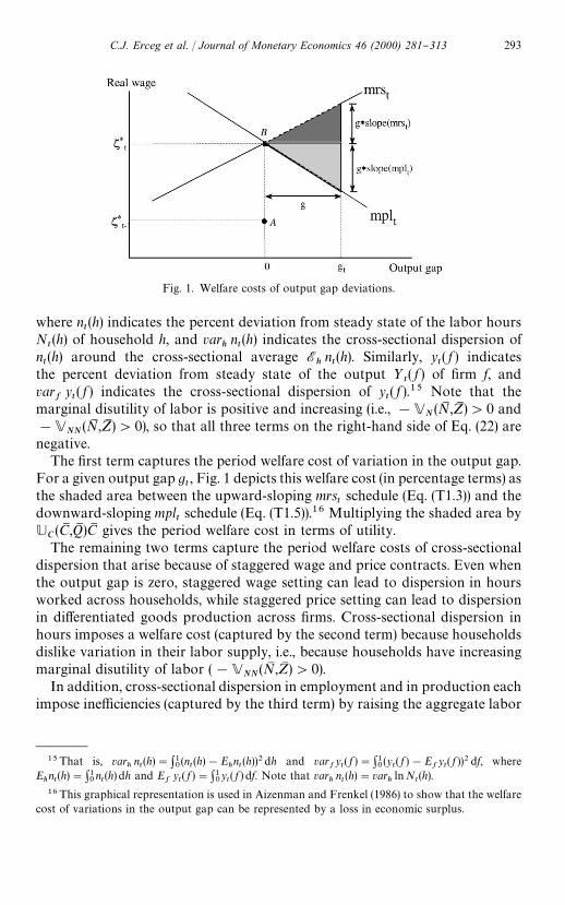
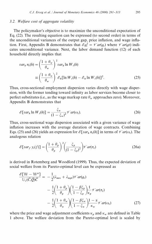
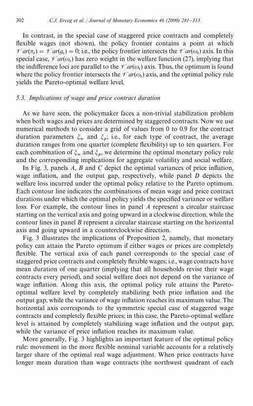
Fig. 1. Welfare costs of output gap deviations.

15That is, varhnt(h)":1

0(n

t(h)!E

hnt(h))2dh and var

fyt( f )":1

0(y

t( f )!E

fyt( f ))2 df, where

Ehnt(h)":1

0nt(h) dh and E

fyt( f )":1

0yt( f ) df. Note that var

hnt(h)"var

hlnN

t(h).

16This graphical representation is used in Aizenman and Frenkel (1986) to show that the welfarecost of variations in the output gap can be represented by a loss in economic surplus.

where nt(h) indicates the percent deviation from steady state of the labor hours

Nt(h) of household h, and var

hnt(h) indicates the cross-sectional dispersion of

nt(h) around the cross-sectional average E

hnt(h). Similarly, y

t( f ) indicates

the percent deviation from steady state of the output >t( f ) of "rm f, and

varf

yt( f ) indicates the cross-sectional dispersion of y

t( f ).15 Note that the

marginal disutility of labor is positive and increasing (i.e., !VN(NM ,ZM )'0 and

!VNN

(NM ,ZM )'0), so that all three terms on the right-hand side of Eq. (22) arenegative.

The "rst term captures the period welfare cost of variation in the output gap.For a given output gap g

t, Fig. 1 depicts this welfare cost (in percentage terms) as

the shaded area between the upward-sloping mrstschedule (Eq. (T1.3)) and the

downward-sloping mpltschedule (Eq. (T1.5)).16 Multiplying the shaded area by

UC(CM ,QM )CM gives the period welfare cost in terms of utility.The remaining two terms capture the period welfare costs of cross-sectional

dispersion that arise because of staggered wage and price contracts. Even whenthe output gap is zero, staggered wage setting can lead to dispersion in hoursworked across households, while staggered price setting can lead to dispersionin di!erentiated goods production across "rms. Cross-sectional dispersion inhours imposes a welfare cost (captured by the second term) because householdsdislike variation in their labor supply, i.e., because households have increasingmarginal disutility of labor (!V

NN(NM ,ZM )'0).

In addition, cross-sectional dispersion in employment and in production eachimpose ine$ciencies (captured by the third term) by raising the aggregate labor


17As a second-order approximation, Eq. (22) omits higher-order terms that involve the interac-tion between productive ine$ciencies and aggregate output #uctuations, as well as higher-orderterms associated with the response of employment dispersion to #uctuations in the labor hours ofthe average household.

hours, Nt":1

0N

t(h) dh, needed to produce a given level of the output index.

These ine$ciencies would arise even if the marginal disutility of labor wereconstant (V

NN(NM ,ZM )"0).17 Labor services of households are imperfect substi-

tutes in production, and di!erentiated goods are imperfect substitutes in con-sumption; thus, the magnitudes of the ine$ciencies increase with the degrees ofconcavity of the labor index and of the output index (as determined by thevalues of the wage markup rate h

wand the price markup rate h

p). Since each

household's labor hours enter symmetrically into the aggregate labor index, andevery household has equal weight in the social welfare function, the Pareto-optimal equilibrium has the property that the number of labor hours is identicalacross households. Under staggered wage setting, however, the economy nolonger exhibits this optimality property. The ine$ciency associated with cross-sectional dispersion of labor hours can be expressed in terms of the percentageincrease in aggregate labor hours required to produce a given level of the laborindex:

nt"l

t#

1

2Ahw

1#hwBvar

hnt(h) (23)

where ntis the percent deviation from steady state of average labor hours, N

t,

and ltis the percent deviation from steady state of the labor index, ¸

t.

Similarly, staggered price setting induces cross-sectional dispersion in produc-tion, and thereby increases the average level of di!erentiated goods outputrequired to produce a given level of the output index. Since all "rms face thesame Cobb}Douglas production function (Eq. (4)), this ine$ciency can beexpressed in terms of the percentage increase in the labor index required toproduce a given level of the output index:

lt"

1

(1!a)(y

t!x

t)#

1

2

1

(1!a)Ahp

1#hpBvar

fyt( f ) (24)

where ytand x

tare the percent deviations from steady state of the output index

>t

and of total factor productivity Xt, respectively. The second term on the

right-hand side of Eq. (24) represents the increased amount of labor hoursrequired because of cross-sectional dispersion in production.

The "nal term in the welfare approximation (Eq. (22)) is obtained by multiply-ing the ine$ciency terms in Eqs. (23) and (24) by the factor V

N(NM ,ZM )NM .


3.2. Welfare cost of aggregate volatility

The policymaker's objective is to maximize the unconditional expectation ofEq. (22). The resulting equation can be expressed (to second order) in terms ofthe unconditional variances of the output gap, price in#ation, and wage in#a-tion. First, Appendix B demonstrates that Eg2

t"Var(g

t) where Var(gt) indi-

cates unconditional variance. Next, the labor demand function (12) of eachhousehold directly implies that

varhnt(h)"A

1#hw

hwB

2var

hln=

t(h)

,A1#h

whwB

2Eh[ln=

t(h)!E

hln=

t(h)]2. (25)

Thus, cross-sectional employment dispersion varies directly with wage disper-sion, with the former tending toward in"nity as labor services become closer toperfect substitutes (i.e., as the wage markup rate h

wapproaches zero). Moreover,

Appendix B demonstrates that

E[varhln=

t(h)]"

mw

(1!mw)2Var(u

t). (26)

Thus, cross-sectional wage dispersion associated with a given variance of wagein#ation increases with the average duration of wage contracts. CombiningEqs. (25) and (26) yields an expression for E[var

hnt(h)] in terms of Var(u

t). The

analogous relation

E[varf

yt( f )]"A

1#hp

hpB

2

Amp

(1!mp)2BVar(n

t) (26a)

is derived in Rotemberg and Woodford (1999). Thus, the expected deviation ofsocial welfare from its Pareto-optimal level can be expressed as

E[W!WH]

Uc(CM ,QM )CM

"!

1

2(j

mrs#j

mpl)Var(g

t)

!

1

2A1#h

phpBA

1!bmp

1!mpB

1

ip

Var(nt)

!

1

2A1#h

whwBA

1!bmw

1!mwB1!aiw

Var(ut) (27)

where the price and wage adjustment coe$cients ip

and iw

are de"ned in Table1 above. The welfare deviation from the Pareto-optimal level is scaled by


18 It is important to note that our log-linear approximation becomes relatively inaccurate as thedegree of substitutability of di!erentiated goods or labor services approaches in"nity, that is, aseither h

por h

wapproach zero.

UC(CM ,QM )CM , so that the right-hand side of Eq. (27) expresses these welfare losses as

a fraction of Pareto-optimal consumption.Several important qualitative features of the social welfare function are

evident from Eq. (27). The welfare cost of price in#ation volatility increases withthe degree of substitutability across di!erentiated goods (which is inverselyrelated to the price markup rate h

p) and with the mean duration of price

contracts (which varies positively with mp

and negatively with ip).18 Welfare is

independent of the variance of price in#ation only in the special case ofcompletely #exible prices (i.e., m

p"0 and hence i

p"R). Similarly, the welfare

cost of wage in#ation volatility increases with the degree of substitutabilityacross di!erentiated labor inputs (which is inversely related to the wage markuprate h

w) and with the mean duration of wage contracts (which varies positively

with mw

and negatively with iw). Finally, it should be noted that the welfare cost

of output gap volatility does not depend on either mpor m

w. Thus, the relative

weight on output gap volatility declines with the mean duration of pricecontracts and the mean duration of wage contracts.

4. The policy frontier

We have shown that the policymaker's welfare function can be expressed interms of the variances of three aggregate variables: the output gap, pricein#ation, and wage in#ation. We demonstrate the impossibility of completelystabilizing more than one of these three variables. This result depends only onthe aggregate supply relations (T1.2)}(T1.5), and not on the particular speci"ca-tion of goods demand or the monetary policy rule. It follows that monetarypolicy cannot achieve the Pareto-optimal level of social welfare. Instead, thepolicymaker faces tradeo!s in stabilizing the three variables; these tradeo!s aresummarized by the policy frontier. The Pareto optimum can be achieved only inthe two special cases in which either prices or wages are completely #exible.

4.1. The general case

Our result for the general case of staggered wage and price setting is stated inthe following proposition:

Proposition 1. With staggered wage and price setting (mw'0 and m

p'0), there

exists a tradeow in stabilizing the output gap, the price inyation rate, and the wage


19According to Eqs. (T1.3) and (T1.5) any shock shifts both schedules vertically by the amount ofthe change in the equilibrium real wage. We consider a positive productivity shock as an example.

inyation rate: it is impossible for more than one of the three variables gt, n

t, and

ut

to have zero variance. Therefore, monetary policy cannot attain the Pareto-optimal social welfare level.

Proof. From Eq. (T1.4), price in#ation remains at steady state if and only if thereal wage and the marginal product of labor are equal; i.e., n

t"n

t`1@t"0 if and

only if ft"mpl

t, where the mpl

tschedule is given by Eq. (T1.2). Similarly, from

Eq. (T1.5), wage in#ation remains at steady state if and only if the real wage andthe marginal rate of substitution are equal; i.e., u

t"u

t`1@t"0 if and only if

ft"mrs

t, where the mrs

tschedule is given by Eq. (T1.3). The mpl

tand mrs

tschedules intersect at the Pareto optimum; i.e., g

t"0 and f

t"fH

tif and only if

ft"mpl

t"mrs

t. Thus, any two of the three conditions (g

t"0, f

t"mpl

t, and

ft"mrs

t) imply the third condition, so that the output gap would remain at

zero and nominal wage in#ation and price in#ation would remain constant onlyif the aggregate real wage rate were continuously at its Pareto-optimal level.However, it is evident from Eq. (19) that the Pareto-optimal real wage fH

tmoves

in response to each of the exogenous shocks, whereas the actual real wageftwould always remain at its steady-state value if neither prices nor wages ever

adjusted. Given this contradiction, it follows that no more than one of the threevariables g

t, n

t, and u

tcan have zero variance when the exogenous shocks have

non-zero variance. Therefore, the Pareto-optimal social welfare level is in-feasible, because the variances of all three variables enter the policymaker'swelfare function with weights that are strictly negative.

The proof is illustrated in Fig. 1. Point A represents an initial Pareto-optimalequilibrium. Point B represents the Pareto-optimal equilibrium following a pos-itive productivity shock.19 Completely stabilizing any two of the three variablesgt, n

t, and u

tis impossible, because doing so would imply that the economy was

simultaneously at both points A and B.

4.2. Two special cases

As noted in the introduction, recent studies have characterized optimalmonetary policy in optimizing-agent models in which staggered price setting isthe sole form of nominal rigidity. The salient "nding of these studies is thatmonetary policy faces no tradeo! between minimizing variability in the outputgap and minimizing variability in price in#ation, so the Pareto optimal welfarelevel can be attained. This "nding is consistent with the implication of the specialcase of our model in which wages are completely #exible. We prove thefollowing proposition:


20See Kiley (1998) and McCallum and Nelson (1999). In the resulting equation, if price in#ation iscompletely stabilized, then the variance of the output gap is proportional to the variance of theexogenous shock.

Proposition 2. (A) With staggered price contracts and completely yexible wages(m

p'0 and m

w"0), monetary policy can completely stabilize price inyation and

the output gap, thereby attaining the Pareto-optimal social welfare level.(B) With staggered wage contracts and completely yexible prices (m

w'0 and

mp"0), monetary policy can completely stabilize wage inyation and the output gap,

thereby attaining the Pareto-optimal social welfare level.

To prove Proposition 2(A), note that in this case, nominal wages can adjustfreely to ensure that the real wage is equal to the marginal rate of substitution(f

t"mrs

t). Combining this condition with Eqs. (T1.2), (T1.3), and (T1.4) yields

an expectational Phillips curve that looks reasonably familiar except for theabsence of an error term:

nt"bn

t`1@t#A

ipK

1!aBgt . (28)

This equation implies that the output gap has zero variance if price in#ation iscompletely stabilized (i.e., g

t"0 if n

t"n

t`1@t"0). Solving Eq. (28) forward

shows that stabilizing the output gap also stabilizes price in#ation. Given thatwages are completely #exible, the variance of wage in#ation receives zero weightin the social welfare function (27). Thus, it is possible to attain the Pareto-optimal social welfare level by strictly targeting either price in#ation (as recom-mended by Goodfriend and King (1997) and King and Wolman (1999)), orequivalently, the output gap.

Proposition 2(A) indicates that staggered price setting by itself does not implya price in#ation}output gap variance tradeo!. To obtain such a tradeo!, oneapproach taken in the literature has been to add an exogenous shock to Eq.(28).20 Such a shock has been interpreted as representing aggregate pricingmistakes or other unexplained deviations from the optimality condition (28). Incontrast, a price in#ation}output gap variance tradeo! arises endogenously inour model with staggered wage and price setting. By substituting the mpl

tschedule (T1.2) into the price-setting equation (T1.4), we obtain the followingrelationship:

nt"bn

t`1@t#i

pjmpl

gt#i

p(f

t!fH

t). (29)

A stabilization tradeo! arises because of the "nal term ip(f

t!fH

t) in Eq. (29),

rather than from an ad hoc shock. Furthermore, this tradeo! depends on thepreference and technology parameters of the model as well as the exogenousdisturbances x

t, q

t, and z

t.


21Examples include Levin (1989), Bryant et al. (1993), Henderson and McKibbin (1993),Blanchard (1997), and Friedman (1999).

22See Erceg et al. (1998). By taking this approach, we also avoid the need to calibrate a contem-poraneous covariance matrix for the three disturbances.

To prove Proposition 2(B), note that prices can adjust freely to ensure that thereal wage is equal to the marginal product of labor (f

t"mpl

t). Combining this

condition with Eqs. (T1.2), (T1.3), and (T1.5) yields the following relationship:

ut"bu

t`1@t#A

iwK

1!aBgt. (30)

Comparison of Eqs. (28) and (30) reveals the formal symmetry between the twospecial cases. Eq. (30) implies that complete wage in#ation stabilization(u

t"u

t`1@t"0) stabilizes the output gap, while prices adjust freely to keep the

real wage at its Pareto-optimal value. Given that the variance of price in#ationdoes not enter the social welfare function (27), it is possible to attain thePareto-optimal social welfare level.

Evidently, in this special case with staggered wage setting and completely#exible prices, complete output gap stabilization generates positive variance ofprice in#ation. Such a variance tradeo! has been derived previously in othermodels with sticky wages and #exible prices.21 Nevertheless, as is evident fromProposition 2(B), this tradeo! does not necessarily have any consequences forsocial welfare.

5. Optimal monetary policy

In this section we use numerical methods to characterize optimal monetarypolicy. In particular, for speci"ed values of the structural parameters, we "nd theinterest rate rule that maximizes the welfare function (27) subject to the log-linearized behavioral equations given in Table 1. For the sake of brevity andclarity, we focus exclusively on volatility induced by exogenous productivityshocks; consumption and leisure shocks imply qualitatively similar properties ofthe monetary policy frontier.22

5.1. Parameterization and computation

Throughout this section, we use a discount factor b of 0.99 (corresponding toa quarterly periodicity of the model), and we use household utility parametersp"s"1.5 (so that utility is nearly logarithmic in consumption and leisure).Unless otherwise speci"ed, the Cobb}Douglas capital share parameter a"0.3


23To determine the general form of the optimal interest rate rule, we followed the approach ofTetlow and von zur Muehlen (1999).

24A detailed description of the solution algorithm and recent enhancements may be found inAnderson (1997). Using Matlab version 5.2 on a 400 Mhz Pentium II, this algorithm generates therational expectations solution within a few seconds for every case considered here.

(implying that output has a labor elasticity of 0.7); the wage and price markuprates h

w"h

p"1

3; and the wage and price contract duration parameters

mw"m

p"0.75 (implying an average contract duration of 1/(1!0.75)"4 quar-

ters). We assume that the productivity shock xtfollows an AR(1) process with

"rst-order autocorrelation of 0.95, where the innovation ex,t

is i.i.d. with meanzero and variance p2ex .

The full model consists of the equations in Table 1 and the optimal interestrate rule. Given our assumptions about the exogenous shocks, the optimalinterest rate rule has the following general form:23

it"c

0nt#c

1it~1

#c2ft~1

#c3xt~1

#c4ex,t#c

5ft~2

#c6xt~2

#c7ex,t~1

.

(31)

It is important to note that this rule includes a "xed parameter c0

on currentprice in#ation n

t; this parameter must be large enough to ensure determinacy

(i.e., the existence of a unique stationary rational expectations equilibrium). Theparticular value chosen for c

0does not a!ect the reduced-form solution when

the other parameters in Eq. (31) are chosen optimally.To con"rm that the determinacy conditions are satis"ed and to compute the

reduced-form solution of the model for a given set of parameters, we use thenumerical algorithm of Anderson and Moore (1985), which provides an e$cientimplementation of the method proposed by Blanchard and Kahn (1980). Havingobtained the reduced-form solution, it is straightforward to compute the vari-ances of the output gap, price in#ation, and wage in#ation. These variances inturn are used to evaluate the welfare function (27). For a given set of structuralparameters, we use a hill-climbing algorithm to determine the values of themonetary policy parameters that maximize social welfare.24 Throughoutthe remainder of the paper, the variances of the endogenous variables andthe corresponding welfare loss are all scaled by the productivity innovationvariance.

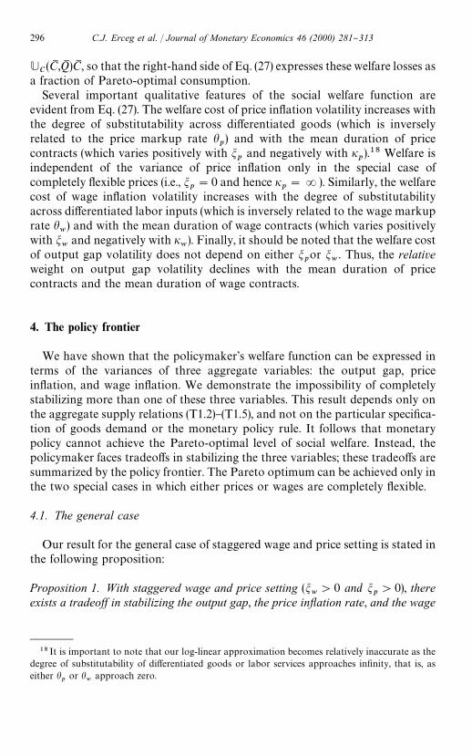
5.2. Geometric representation

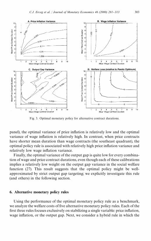
Using the numerical methods described above, we can depict the policy-maker's optimization problem geometrically, thereby highlighting the parallelswith the standard social planner's problem. In particular, each level set of the


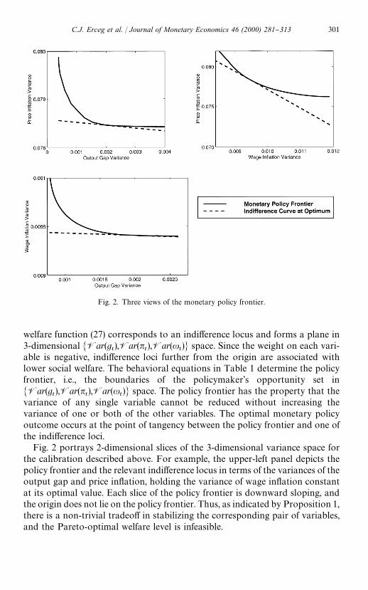
Fig. 2. Three views of the monetary policy frontier.

welfare function (27) corresponds to an indi!erence locus and forms a plane in3-dimensional MVar(g

t),Var(n

t),Var(u

t)N space. Since the weight on each vari-

able is negative, indi!erence loci further from the origin are associated withlower social welfare. The behavioral equations in Table 1 determine the policyfrontier, i.e., the boundaries of the policymaker's opportunity set inMVar(g

t),Var(n

t),Var(u

t)N space. The policy frontier has the property that the

variance of any single variable cannot be reduced without increasing thevariance of one or both of the other variables. The optimal monetary policyoutcome occurs at the point of tangency between the policy frontier and one ofthe indi!erence loci.

Fig. 2 portrays 2-dimensional slices of the 3-dimensional variance space forthe calibration described above. For example, the upper-left panel depicts thepolicy frontier and the relevant indi!erence locus in terms of the variances of theoutput gap and price in#ation, holding the variance of wage in#ation constantat its optimal value. Each slice of the policy frontier is downward sloping, andthe origin does not lie on the policy frontier. Thus, as indicated by Proposition 1,there is a non-trivial tradeo! in stabilizing the corresponding pair of variables,and the Pareto-optimal welfare level is infeasible.


In contrast, in the special case of staggered price contracts and completely#exible wages (not shown), the policy frontier contains a point at whichVar(n

t)"Var(g

t)"0; i.e., the policy frontier intersects the Var(u

t) axis. In this

special case, Var(ut) has zero weight in the welfare function (27), implying that

the indi!erence loci are parallel to the Var(ut) axis. Thus, the optimum is found

where the policy frontier intersects the Var(ut) axis, and the optimal policy rule

yields the Pareto-optimal welfare level.

5.3. Implications of wage and price contract duration

As we have seen, the policymaker faces a non-trivial stabilization problemwhen both wages and prices are determined by staggered contracts. Now we usenumerical methods to consider a grid of values from 0 to 0.9 for the contractduration parameters m

wand m

p; i.e., for each type of contract, the average

duration ranges from one quarter (complete #exibility) up to ten quarters. Foreach combination of m

wand m

p, we determine the optimal monetary policy rule

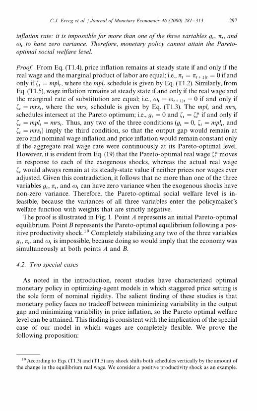
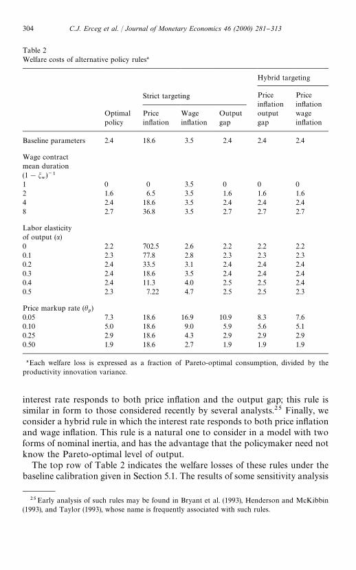
and the corresponding implications for aggregate volatility and social welfare.In Fig. 3, panels A, B and C depict the optimal variances of price in#ation,

wage in#ation, and the output gap, respectively, while panel D depicts thewelfare loss incurred under the optimal policy relative to the Pareto optimum.Each contour line indicates the combinations of mean wage and price contractdurations under which the optimal policy yields the speci"ed variance or welfareloss. For example, the contour lines in panel A represent a circular staircasestarting on the vertical axis and going upward in a clockwise direction, while thecontour lines in panel B represent a circular staircase starting on the horizontalaxis and going upward in a counterclockwise direction.

Fig. 3 illustrates the implications of Proposition 2, namely, that monetarypolicy can attain the Pareto optimum if either wages or prices are completely#exible. The vertical axis of each panel corresponds to the special case ofstaggered price contracts and completely #exible wages; i.e., wage contracts havemean duration of one quarter (implying that all households revise their wagecontracts every period), and social welfare does not depend on the variance ofwage in#ation. Along this axis, the optimal policy rule attains the Pareto-optimal welfare level by completely stabilizing both price in#ation and theoutput gap, while the variance of wage in#ation reaches its maximum value. Thehorizontal axis corresponds to the symmetric special case of staggered wagecontracts and completely #exible prices; in this case, the Pareto-optimal welfarelevel is attained by completely stabilizing wage in#ation and the output gap,while the variance of price in#ation reaches its maximum value.

More generally, Fig. 3 highlights an important feature of the optimal policyrule: movement in the more #exible nominal variable accounts for a relativelylarger share of the optimal real wage adjustment. When price contracts havelonger mean duration than wage contracts (the northwest quadrant of each


Fig. 3. Optimal monetary policy for alternative contract durations.

panel), the optimal variance of price in#ation is relatively low and the optimalvariance of wage in#ation is relatively high. In contrast, when price contractshave shorter mean duration than wage contracts (the southeast quadrant), theoptimal policy rule is associated with relatively high price in#ation variance andrelatively low wage in#ation variance.

Finally, the optimal variance of the output gap is quite low for every combina-tion of wage and price contract durations, even though each of these calibrationsimplies a relatively low weight on the output gap variance in the social welfarefunction (27). This result suggests that the optimal policy might be well-approximated by strict output gap targeting; we explicitly investigate this rule(and others) in the following section.

6. Alternative monetary policy rules

Using the performance of the optimal monetary policy rule as a benchmark,we analyze the welfare costs of "ve alternative monetary policy rules. Each of the"rst three rules focuses exclusively on stabilizing a single variable: price in#ation,wage in#ation, or the output gap. Next, we consider a hybrid rule in which the


Table 2Welfare costs of alternative policy rules!

Strict targeting

Hybrid targeting

Optimalpolicy

Pricein#ation

Wagein#ation

Outputgap

Pricein#ationoutputgap

Pricein#ationwagein#ation

Baseline parameters 2.4 18.6 3.5 2.4 2.4 2.4

Wage contractmean duration(1!m

w)~1

1 0 0 3.5 0 0 02 1.6 6.5 3.5 1.6 1.6 1.64 2.4 18.6 3.5 2.4 2.4 2.48 2.7 36.8 3.5 2.7 2.7 2.7

Labor elasticityof output (a)0 2.2 702.5 2.6 2.2 2.2 2.20.1 2.3 77.8 2.8 2.3 2.3 2.30.2 2.4 33.5 3.1 2.4 2.4 2.40.3 2.4 18.6 3.5 2.4 2.4 2.40.4 2.4 11.3 4.0 2.5 2.5 2.40.5 2.3 7.22 4.7 2.5 2.5 2.3

Price markup rate (hp)

0.05 7.3 18.6 16.9 10.9 8.3 7.60.10 5.0 18.6 9.0 5.9 5.6 5.10.25 2.9 18.6 4.3 2.9 2.9 2.90.50 1.9 18.6 2.7 1.9 1.9 1.9

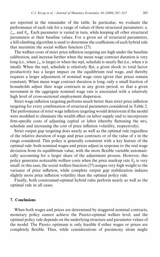
!Each welfare loss is expressed as a fraction of Pareto-optimal consumption, divided by theproductivity innovation variance.

25Early analysis of such rules may be found in Bryant et al. (1993), Henderson and McKibbin(1993), and Taylor (1993), whose name is frequently associated with such rules.

interest rate responds to both price in#ation and the output gap; this rule issimilar in form to those considered recently by several analysts.25 Finally, weconsider a hybrid rule in which the interest rate responds to both price in#ationand wage in#ation. This rule is a natural one to consider in a model with twoforms of nominal inertia, and has the advantage that the policymaker need notknow the Pareto-optimal level of output.

The top row of Table 2 indicates the welfare losses of these rules under thebaseline calibration given in Section 5.1. The results of some sensitivity analysis


are reported in the remainder of the table. In particular, we evaluate theperformance of each rule for a range of values of three structural parameters: a,mw, and h

p. Each parameter is varied in turn, while keeping all other structural

parameters at their baseline values. For a given set of structural parameters,a hill-climbing algorithm is used to determine the coe$cients of each hybrid rulethat maximize the social welfare function (27).

The welfare costs of strict price in#ation targeting are high under the baselinecalibration, and increase further when the mean wage contract duration is verylong (i.e., when m

wis large) or when the mpl

tschedule is nearly #at (i.e., when a is

small). When the mplt

schedule is relatively #at, a given shock to total factorproductivity has a larger impact on the equilibrium real wage, and therebyrequires a larger adjustment of nominal wage rates (given that prices remainconstant). When mean wage contract duration is long, only a small fraction ofhouseholds adjust their wage contracts in any given period, so that a givenmovement in the aggregate nominal wage rate is associated with a relativelyhigh level of cross-sectional employment dispersion.

Strict wage in#ation targeting performs much better than strict price in#ationtargeting for every combination of structural parameters considered in Table 2.The performance of strict wage in#ation targeting would deteriorate if the modelwere modi"ed to eliminate the wealth e!ect on labor supply and to incorporate"rm-speci"c costs of adjusting capital or labor (thereby #attening the mrs

tschedule and increasing the cost of price in#ation volatility, respectively).

Strict output gap targeting does nearly as well as the optimal rule regardlessof the relative duration of wage and price contracts or of the value of a in therange considered. This policy is generally consistent with a key feature of theoptimal rule: both nominal wages and prices adjust in response to the real wagedeviation from its equilibrium value, with the more #exible variable automati-cally accounting for a larger share of the adjustment process. However, thispolicy generates noticeable welfare costs when the price markup rate h

pis very

small: in this case, the social welfare function (27) assigns very high weight to thevariance of price in#ation, while complete output gap stabilization inducesslightly more price in#ation volatility than the optimal policy rule.

Finally, both constrained-optimal hybrid rules perform nearly as well as theoptimal rule in all cases.

7. Conclusions

When both wages and prices are determined by staggered nominal contracts,monetary policy cannot achieve the Pareto-optimal welfare level, and theoptimal policy rule depends on the underlying structure and parameter values ofthe model. The Pareto optimum is only feasible if either wages or prices arecompletely #exible. Thus, while considerations of parsimony alone might


26Barro (1977) is sometimes cited to support this view. However, Barro himself applies thisargument to prices as well as wages.

suggest an exclusive focus on either staggered price setting or staggered wagesetting, the inclusion of both types of nominal inertia makes a critical di!erencein the monetary policy problem.

More generally, our analysis suggests that the existence of a monetary policytradeo! is not contingent on the particular speci"cation of staggered wageand price setting considered here. For example, our model is isomorphic toa model with di!erentiated goods at two stages of production, in which theprices of both intermediate inputs and "nal goods are determined by staggerednominal contracts. We conjecture that a monetary policy tradeo! would alsoexist under alternative formulations, such as (1) one-period input pricecontracts and staggered output price contracts, and (2) #exible input prices andstaggered output price contracts, where di!erentiated goods producers faceidiosyncratic productivity shocks or shifts in relative demand. In each of thesecases, the prices of several inputs and/or outputs are determined by nominalcontracts that are not completely synchronized, and some of the relative pricesof these items vary in response to exogenous shocks in the Pareto-optimalequilibrium.

Although it is worthwhile to consider alternative formulations of nominalinertia, we believe that both wages and prices are sticky in actual economies,and that the relative price of labor plays an important role in generatinga non-trivial policy tradeo!. Our position is consistent with the long historyof analyses (dating back at least to Keynes (1935)) in which nominal wage inertiaplays a signi"cant role in generating aggregate #uctuations. In contrast,recent contributions have emphasized sticky prices rather than sticky wages, atleast in part because state-contingent employment contracts can, in principle,prevent any misallocation of labor due to nominal wage contracts.26 However,one can also imagine state-contingent output contracts which ensure that stickyprices have no allocative e!ects; such state-contingent contracts are neithermore nor less plausible than the analogous employment contracts. Hence, itseems reasonable to assume that both wage and price contracts have signi"cantallocative e!ects, at least until further guidance is provided by empiricalresearch.

We have used numerical methods to analyze the properties of optimalmonetary policy and to quantify the welfare losses of alternative policy rules.For the speci"cations considered here, we "nd that strict price in#ation target-ing generates relatively large welfare losses, whereas several other simple policyrules perform nearly as well as the optimal rule. These "ndings should beinvestigated further in models that relax some of our key simplifying


27Other key simplifying assumptions include time-separable preferences, no capital accumula-tion, no adjustment costs, and exogenous duration of wage and price contracts. The sensitivity ofcontract duration to monetary policy has been studied previously by Canzoneri (1980), Gray (1978),and Dotsey et al. (1997), among others.

assumptions such as complete consumption risk sharing and complete informa-tion of private agents and policymakers.27

Appendix A

In this appendix, we derive the aggregate wage-setting equation (T1.5) using"rst-order Taylor approximations where appropriate. For every householdhIt

that resets its contract wage in period t, de"ne dt(hI

t)"ln=

t(hI

t)!ln=

t.

Then the log di!erential of the "rst-order condition (16) around the steadystate is

dt(hI

t)

1!mwb#E

t+

=

j/0

mjwbj(f

t`j#UK

C,t`j#VK

N,t`j(hI

t)!+

j

k/1

ut`k

)"0.

(A.1)

Using the labor demand Eq. (12), we can rewrite VKN,t`j

(hIt) as

VKN,t`j

(hIt)"VK

N,t`j#sl

NA1#h

whwBAdt (hI t )!

j+k/1

ut`kB (A.2)

where !VKN,t`j

"s(lNlt#l

Zzt) is the average of marginal disutilities of labor

across households. Eq. (18) implies that mrst"!(UK

C,t#VK

N,t), while the ag-

gregate wage de"nition (11) implies that dt(hI

t)"(m

w/(1!m

w))u

t. Thus, substitu-

ting (A.2) into (A.1) yields

mw

(1!mw)(1!m

wb)

ut"E

t

=+j/1

mjwbj

j+k/1

ut`k

#Et

=+j/0

mjwbjA

mrst`j

!ft`j

1#(1`hwhw )slNB .

(A.3)

Forwarding (A.3) by one period, multiplying the result by mwb, subtracting the

outcome from (A.3), and rearranging yields (T1.5).

Appendix B

In this appendix, we derive the approximation of Wt!WH

tgiven in Eq. (22).

We also show that Eg2t"Var(g

t) and that E[var

hMln=

t(h)N]"

(mw/(1!m

w)2)Var(u

t) (see equation (26)). Throughout this appendix, we use

second-order Taylor approximations.


We use two approximations repeatedly. If A is a generic variable, the relation-ship between its arithmetic and logarithmic percentage changes is

A!AMAM

"

dA

AMKa#

1

2a2, a,lnA!lnAM (B.1)

If A"[:10A( j )(dj]1@(, the logarithmic approximation of A is

aKEja( j )#1

2/(E

ja( j )2!(E

ja( j ))2)"E

ja( j )#1

2/var

ja( j ). (B.2)

B.1. The derivation of the approximation of W!WH

Eq. (21) without time subscripts is repeated here for convenience:

W"U(C,Q)#P1

0

V(N(h),Z) dh"U(C,Q)#EhV(N(h),Z). (B.3)

First, we approximate U(C,Q):

U(C,Q)KUM #UCCM

dC

CM#U

QQM

dQ

QM

#

1

2AUCCCM 2A

dC

CM B2#2U

CQCM QM

dC

CMdQ

QM#U2

QQQM 2A

dQ

QM B2

B.(B.4)

Making use of result (B.1) yields

U(C,Q)KUM #UCCM (y#1

2y2)#U

QQM (q#1

2q2)

# 12(U

CCCM 2y2#2U

CQCM QM yq#U2

QQQM 2q2). (B.5)

Next we approximate EhV(N(h),Z):

EhV(N(h),Z)KVM #E

hV

NNM

dN(h)

NM#V

ZZM

dZ

ZM

#

1

2AEhV

NNNM 2A

dN(h)

NM B2#E

hV

NZNM ZM

dN(h)

NMdZ

ZM

#VZZ

ZM 2AdZ

ZM B2

B (B.6)


Making use of result (B.1) yields

EhV(N(h),Z)KVM #V

NNM (E

hn(h)#1

2E

hn(h)2)#V

ZZM (z#1

2z2)

# 12(V

NNNM 2E

hn(h)2#2V

NZNM ZM zE

hn(h)#V

ZZZM 2z2).

(B.7)

The aggregate supply of labor by households is ¸"[:10N(h)1@(1`hw )dh]1`hW .

Thus,

l"lnCP1

0

N(h)1@(1`hw ) dhD1`hw

!ln M̧ KEhn(h)

#

1

2A1

1#hwBvar

hn(h). (B.8)

The aggregate demand for labor by "rms is ¸":10¸( f ) df"E

f¸( f ). Thus,

l"lnEf¸( f )!ln M̧ KE

fl( f )#1

2var

fl( f ). (B.9)

All "rms choose identical capital labor ratios (K( f )/¸( f )) equal to the aggregateratio (K/¸) because they face the same factor prices, so

>( f )"AK( f )

¸( f )Ba¸( f )X"A

K

¸Ba¸( f )X. (B.10)

Since the total amount of capital is "xed, Eq. (B.10) in turn implies

y( f )"x!al#l( f ), Ef

y( f )"x!al#Efl( f ),

varf

y( f )"varf

l( f ). (B.11)

Substituting the relationships in Eq. (B.11) into Eq. (B.9), and eliminatingEfy( f )

using Eq. (B.2) yields Eq. (24), repeated here for convenience:

lK1

1!a(y!x)#

1

2A1

1!aBAhp

1#hpBvar

fy( f ). (B.12)

Solving Eq. (B.8) for Ehn(h) and eliminating l using Eq. (B.12) yields

Ehn(h)K

1

1!a(y!x)#

1

2A1

1!aBAhp

1#hpBvar

fy( f )

!

1

2A1

1#hwBvar

hn(h). (B.13)


Using the relationship Ehn(h)2"var

hn(h)#[E

hn(h)]2 to eliminate E

hn(h)2, and

Eq. (B.13) to eliminate Ehn(h), Eq. (B.7) can be rewritten as

EhV(N(h),Z) dhKVM #V

ZZM z#V

NNM A

y!x

1!aB#

1

2C(VZZM #V

ZZZM 2)z2#2V

NZNM ZM A

(y!x)z

1!a B# (V

NNM #V

NNNM 2)A

y!x

1!aB2

#AVNNM A

hw

1#hwB#V

NNNM 2Bvar

hn(h)

#AV

NNM

1!aBAhp

1#hpBvar

fy(

f)D. (B.14)

Approximating the utility associated with consumption and labor at thePareto optimum, U(CH, Q) and E

hV(NH(h), Z), respectively, in analogous ways

and subtracting the sum of the results from the sum of Eqs. (B.5) and (B.14)yields

W!WHKA!(V

NNM #V

NNNM 2)

(1!a)2x#U

CQCM QM q#

VNZ

NM ZM1!a

zB(y!yH)

#

1

2AUCCM #U

CCCM 2#

VNNM #V

NNNM 2

(1!a)2 B(y2!yH2)

#

1

2AVNNM A

hw

1#hwB#V

NNNM 2Bvar

hn(h)

#

1

2

VNNM

1!aAhp

1#hpBvar

fy( f ) (B.15)

since the "rst-order condition (17) implies that UCCM #V

NNM /(1!a)"0. Our

model implies that UC"(C!Q)~p, U

CC"!U

CQ"!p(C!Q)~p~1,

VN"!(1!N!Z)~s, and V

NN"<

NZ"!s(1!N!Z)~s~1. Thus,

UCC

/UC"!U

CQ/U

C"!p/(C!Q) and V

NN/V

N"V

NZ/V

N"s/(1!N!Z).

Using these relationships together with the solution for Pareto-optimal output(19), the "rst and second lines can be expressed as (KU

CCM /(1!a))yH(y!yH) and

(KUCCM /2(1!a))(yH2!y2), respectively. Combining terms we arrive at Eq. (22).

B.2. Proof that Eg2t"Var(g

t)

Now we show thatEgtis of second order, so that (Eg

t)2 can be neglected in the

second-order approximation. We assume that the model has a unique stationary


solution, so that the deviation of aggregate output>tfrom the Pareto optimum

>Ht

can be expressed as >t!>H

t"B(g

t,g

t~1,g

t~2,2), where g

tis the vector of

mean-zero i.i.d. innovations at time t. Because the economy with staggeredcontracts has the same steady state as the Pareto-optimal economy,B(0,0,0,2)"0. Thus, taking unconditional expectations of the second-orderTaylor approximation yields

EA>

t!>H

t>M B"

1

2>M=+j/0

Bgt~j ,gt~jVar(g

t). (B.16)

Applying expression (B.1) to>t!>H

t, taking unconditional expectations, and

rearranging terms yields

Egt"EA

>t!>H

t>M B!

1

2[Var(g

t)#(Eg

t)2]. (B.17)

Taken together, Eqs. (B.16) and (B.17) imply that Egtis of second order.

B.3. The Approximation of EvarhMln=

t(h)N

As in Appendix A, let =t(hI

t) indicate the wage of every household hI

tthat

resets its contract wage in period t, and let dt(hI

t)"ln=

t(hI

t)!ln=

t. Note that

ln=t(h)"ln=

t~1(h)#lnP for each of the remaining m

whouseholds that

cannot reset their wages. Thus, cross-sectional wage dispersion is

varhln=

t(h)"m

wEh(ln=

t~1(h)#lnP!E

hln=

t(h))2

# (1!mw)(ln=

t(hI

t)!E

hln=

t(h))2. (B.18)

For those households that cannot reset their wages, the wage dispersionaround the current aggregate wage is

Eh(ln=

t~1(h)#ln P!E

hln=

t(h))2"var

hln=

t~1(h)#u2

t(B.19)

because ut,ln=

t!ln=

t~1!lnP and because (E

hln=

t(h)!ln=

t) and

(Ehln=

t(h)!ln=

t) are of second order from (B.2) so their squares and cross

products can be ignored in the second-order approximation.Similarly, (ln=

t(hI

t)!E

hln=

t(h))2"(d

t(hI

t))2. Thus, the squared logarithmic

deviation of the contract wage from the current aggregate wage is

(ln=t(hI

t)!E

hln=

t(h))2"A

mw

1!mwB

2u2

t. (B.20)

Substituting Eqs. (B.19) and (B.20) into Eq. (B.18) and rearranging terms, weobtain

varhln=

t(h)"m

wvar

hln=

t~1(h)#

mw

1!mw

u2t. (B.21)


Finally, taking unconditional expectations and rearranging terms yields

E varhln=

t(h)"

mw

(1!mw)2Eu2

t"

mw

(1!mw)2Var(u

t). (B.22)

Note that Eu2t"Var(u

t) because Eu

t(like Eg

t) is of second order.

References

Aizenman, J., Frenkel, J.A., 1986. Wage indexation, supply shocks, and monetary policy in a smallopen economy, In: Edwards, S., Ahamed, L. (Eds.), Economic Adjustment and Exchange RateChanges in Developing Countries. University of Chicago Press, Chicago.

Anderson, G.S., Moore, G., 1985. A linear algebraic procedure for solving linear perfect foresightmodels. Economic Letters 17, 247}252.

Barro, R.J., 1977. Long-term contracting, sticky prices, and monetary policy. Journal of MonetaryEconomics 3, 305}316.

Blanchard, O., 1997. Comment, In: NBER Macroeconomics Annual 1997. MIT Press, Cambridge,MA, pp. 289}295.

Blanchard, O., Kahn, C.M., 1980. The solution of linear di!erence models under rational expecta-tions. Econometrica 48, 1305}1311.

Blanchard, O.J., Kiyotaki, N., 1987. Monopolistic competition and the e!ects of aggregate demand.American Economic Review 77 (4), 647}666.

Bryant, R., Hooper, P., Mann, C., 1993. Evaluating Policy Regimes: New Research in EmpiricalMacroeconomics. Brookings Institution, Washington, D.C.

Calvo, G., 1983. Staggered prices in a utility maximizing framework. Journal of Monetary Econ-omics 12, 383}398.

Canzoneri, M.B., 1980. Labor contracts and monetary policy. Journal of Monetary Economics 6,241}245.

Cuddington, J.T., Johansson, P.-O., LoK fgren, K.-G., 1984. Disequilibrium Macroeconomics in OpenEconomies. Basil Blackwell, Oxford.

Dixit, A.K., Stiglitz, J., 1977. Monopolistic competition and optimum product diversity. AmericanEconomic Review 67, 297}308.

Dotsey, M., King, R.G., Wolman, A.L., 1997. State dependent pricing and dynamics of businesscycles. Working paper No. 97-2, Federal Reserve Bank of Richmond.

Erceg, C.J., 1997. Nominal wage rigidities and the propagation of monetary disturbances. Interna-tional Finance Discussion Papers, No. 590, Federal Reserve Board.

Erceg, C.J., Henderson, D.W., Levin, A.T., 1998. Tradeo!s between in#ation and output-gapvariances in a optimizing-agent model. International Finance Discussion Papers, No. 627,Federal Reserve Board.

Friedman, B., 1999. Comment. In: Taylor, J. (Ed.), Monetary Policy Rules. The University ofChicago Press, Chicago, pp. 398}402.

Goodfriend, M., King, R., 1997. The new neoclassical synthesis and the role of monetary policy. In:Bernanke, B.S., Rotemberg, J.J. (Eds.), NBER Macroeconomics Annual 1997. MIT Press,Cambridge, pp. 233}283.

Gray, J., 1978. On indexation and contract length. Journal of Political Economy 86, 1}18.Henderson, D., McKibbin, W., 1993. A comparison of some basic monetary policy regimes for open

economies: implications of di!erent degrees of instrument adjustment and wage persistence.Carnegie-Rochester Series on Public Policy 39, 221}317.

Ireland, P.N., 1997. A small structural, quarterly model for monetary policy evaluation. Carnegie-Rochester Series on Public Policy 47, 83}108.


Kerr, W., King, R.G., 1996. Limits on interest rate rules in the IS model. Federal Reserve Bank ofRichmond Economic Quarterly 82, 47}75.

Keynes, J.M., 1935. The General Theory of Employment, Interest, and Money. Harcourt, Brace, andWorld, New York.

Kiley, M.T., 1998. Monetary policy under neoclassical and new-Keynesian Phillips curves, with anapplication to price level and in#ation targeting. Finance and Economics Discussion Series No.1998-27, Federal Reserve Board.

Kim, J., 2000. Constructing and estimating a realistic optimizing model of monetary policy. Journalof Monetary Economics 45, 329}359.

Kimball, M.S., 1995. The quantitative analysis of the basic neomonetarist model. Journal of Money,Credit, and Banking 27, 1241}1277.

King, R.G., Wolman, A.L., 1999. What should the monetary authority do when prices are sticky?. In:Taylor, J. (Ed.), Monetary Policy Rules. The University of Chicago Press, Chicago, pp. 349}398.

Kollmann, R., 1997. The exchange rate in a dynamic-optimizing current account model withnominal rigidities: a quantitative investigation. Working paper, International Monetary Fund.

Levin, A., 1989. The theoretical and empirical relevance of staggered wage contract models. Ph.D.Dissertation, Stanford University.

Levin, A., Wieland, V., Williams, J.C., 1999. Robustness of simple monetary policy rules under modeluncertainty. In: Taylor, J. (Ed.), Monetary Policy Rules. The University of Chicago Press,Chicago, pp. 263}299.

McCallum, B.T., Nelson, E., 1999. Performance of operational policy rules in an estimated semiclas-sical structural model. In: Taylor, J. (Ed.), Monetary Policy Rules. The University of ChicagoPress, Chicago, pp. 349}398.

Phelps, E.S., Taylor, J.B., 1977. Stabilizing powers of monetary policy under rational expectations.Journal of Political Economy 85, 163}190.

Rotemberg, J.J., 1996. Prices, output, and hours: an empirical analysis based on a sticky price model.Journal of Monetary Economics 37, 505}533.

Rotemberg, J.J., Woodford, M., 1997. An optimization-based econometric framework for theevaluation of monetary policy. In: Bernanke, B.S., Rotemberg, J.J. (Eds.), NBER Macroeco-nomics Annual 1997. MIT Press, Cambridge, pp. 297}346.

Rotemberg, J.J., Woodford, M., 1999. Interest-rate rules in an estimated sticky price model. In:Taylor, J. (Ed.), Monetary Policy Rules. The University of Chicago Press, Chicago, pp. 57}119.

Rudebusch, G.D., Svensson, L.E.O., 1999. Policy rules for in#ation targeting. In: Taylor, J. (Ed.),Monetary Policy Rules. The University of Chicago Press, Chicago, pp. 203}246.

Solow, R., Stiglitz, J., 1968. Output, employment, and wages in the short run. Quarterly Journal ofEconomics 82, 537}560.

Taylor, J., 1979. Staggered contracts in a macro model. American Economic Review 69, 108}113.Taylor, J., 1980. Aggregate dynamics and staggered contracts. Journal of Political Economy 88, 1}24.Taylor, J.B., 1993. Discretion versus policy rules in practice. Carnegie-Rochester Series on Public

Policy 39, 195}214.Tetlow, R., von zur Muehlen, P., 1996. Monetary policy rules in a small forward-looking maco

model. Processed, Federal Reserve Board.Tetlow, R., von zur Muehlen, P., 1999. Simplicity versus optimality: the choice of monetary policy

rules when agents must learn, Finance and Economics Discussion Series No. 1999-10, FederalReserve Board.

Williams, J.C., 1999. Simple rules for monetary policy. Finance and Economics Discussion SeriesNo. 1999-12, Federal Reserve Board.

Woodford, M., 1996. Control of the public debt: a requirement for price stability?. NBER WorkingPaper 5684, National Bureau of Economic Research.

Yun, T., 1996. Nominal price rigidity, money supply endogeneity, and business cycles. Journal ofMonetary Economics 37, 345}370.


Date post:	29-May-2018
Category:	Documents
Upload:	dinhmien
View:	214 times
Download:	0 times

Optimal monetary policy with staggered wage and price ...yashiv/Erceg et al.pdf · Federal Reserve...

Documents