Optimal Multi-scale Capacity Planning for

Power-Intensive Continuous Processes under

Time-sensitive Electricity Prices and Demand

Uncertainty, Part I: Modeling

Sumit Mitra∗, Jose M. Pinto†, Ignacio E. Grossmann∗‡

May 22, 2013

Abstract

With the advent of deregulation in electricity markets and an in-creasing share of intermittent power generation sources, time-sensitiveelectricity prices (as part of so-called demand-side management in thesmart grid) offer potential economical incentives for large industrialcustomers. These incentives have to be analyzed from two perspec-tives. First, on an operational level, aligning the production planningwith the electricity price signal might be advantageous, if the plant hasenough flexibility to do so. Second, on a strategic level, investmentsin retrofits of existing plants, such as installing additional equipment,upgrading existing equipment, or increasing product storage capacity,facilitate cost savings on the operational level by increasing operationalflexibility.

In part I of this paper, we propose an MILP formulation that in-tegrates the operational and strategic decision-making for continuouspower-intensive processes under time-sensitive electricity prices. Wedemonstrate the trade-off between capital and operating expenditureswith an industrial case study for an air separation plant. Further-more, we compare the insights obtained from a model that assumesdeterministic demand with those obtained from a stochastic demandmodel. The value of the stochastic solution (VSS) is discussed, whichcan be significant in cases with an unclear setup, such as mediumbaseline product demand and growth rate, large variance or skeweddemand distributions. While the resulting optimization models arevery large-scale, they can mostly be solved within up to three days ofcomputational time. A decomposition algorithm that allows solvingthe problems faster is described in part II of the paper.

∗Center for Advanced Process Decision-making, Department of Chemical Engineering,Carnegie Mellon University, Pittsburgh, PA 15213†Praxair Inc., Danbury, CT‡Corresponding author. Email address: grossmann@cmu.edu

1

1 Background

1.1 Motivation

The manufacturing base in the U.S. has been eroding over the last twodecades in the face of fierce international competition. However, recent de-velopments such as the gas production from very large deposits of shale gas(Chang, 2010), as well as trends in onshoring due to rising labor cost inemerging countries (Sirkin et al., 2011), provide hope in the revitalization ofU.S. manufacturing. While the economic recovery deserves further observa-tion in the aftermath of the recession of 2008 and the current unemploymentand financial market volatility, future competitiveness of industrial compa-nies requires them to optimally design and retrofit their production facilitiesin anticipation of price and demand growth forecasts.

A group of chemical processes for which the design and capacity plan-ning is very challenging is the group of power-intensive processes, such as airseparation plants (compression), cement production (grinding), chlor-alkalisynthesis, steel and aluminum production (electrolysis) and paper pulp pro-duction (drying). These industries in fact consume 15% of the total indus-trial electric power in the United States.

At the same time, the power grid is in transition to the so-called smartgrid with the ambition to improve reliability, energy security, economics andgreenhouse gas emissions (Samad and Kiliccote, 2012). A growing shareof intermittent renewable energies, such as wind and solar, increases thechallenge that grid operators face every day and every minute: balancingsupply and demand of electricity on a real-time basis. A set of measures,such as co-generation, micro-grids, future storage technologies and demand-side management (DSM), is expected to play an important role in helpingtoday’s power grid, mastering the transition to the smart grid.

The societal benefit of DSM in the US is estimated to be $59 Billionby 2019, of which 40% is attributed to large commercial and industrial con-sumers (McKinsey study by Davito, Tai and Uhlaner, 2010). Hence, from anindustrial consumer’s perspective, demand-side management (DSM), con-sisting of Energy Efficiency (EE) and Demand Response (DR), deservesspecial attention. The idea of DSM is to influence the “amount and/ortiming of the customers use of electricity for the collective benefit of the so-ciety, the utility and its customers” (Charles River Associates, 2005). WhileEE aims for permanently reducing demand for energy, DR focuses on theoperational level (Voytas et al., 2007).

As a consequence, variability in time-sensitive electricity prices can beobserved on various time scales, including hourly variations for so-calledday-ahead (DA) prices that industrial consumers are exposed to in manyelectricity markets around the globe. However, economic benefits can berealized if the industrial consumer has the flexibility to adjust consumption

2

Figure 1: DSM potential for residential, commercial and industrialsectors in the US.

(Mitra et al., 2012a).Interestingly, industrial DR still seems to be a large untapped grid re-

source according to data released by the Energy Information Administration(EIA, 2010). The EIA investigates the actual and potential peak load reduc-tion (in MW) attributed to DR. While nearly 80 % of the DR potential inthe residential and in the commercial sectors was realized throughout 2006-2010, only 50-60% of the DR potential was accessed in the industrial sector,as one can see in Fig. 1. We conjecture that this data can be explained bythe fact that DSM is part of a complex multi-scale design, capacity planningand operations problem, which requires a sufficient set of decision-makingsupport tools in order to facilitate optimal decisions.

With pressure on both sides, the revenue side (uncertainty in productdemand) and the cost side (variability in electricity prices), new designsand plant retrofits can be viable options for power-intensive processes inthe context of DSM. Retrofitting includes replacing existing equipment withmore energy-efficient alternatives, improving design flexibility (with respectto DR incentives), adding further production equipment and installing ad-ditional storage tanks. All these design decisions, which could potentiallylead to lower operating costs, are part of strategic capacity planning of thechemical companies. Typically, the financial analysis in terms of net presentvalue (NPV) or return on investment (ROI) for the investment decisionsis performed for a time horizon of multiple years, e.g. 10-15 years. Thus,

3

investigating the trade-off between the capital investment costs for new de-signs or retrofits, and the operating costs related to electricity prices, whichcan vary on an hourly basis, leads to a complex multi-scale optimizationproblem.

1.2 Literature review

Multi-period design and capacity planning for continuous multi-productplants has been widely studied in the literature. Sahinidis et al. (1989)propose a comprehensive deterministic MILP model for process networks.Liu and Sahinidis (1996) extend the model to account for demand uncer-tainty. Van den Heever and Grossmann (1999) use disjunctive programmingtechniques to extend the methodology to the case of multi-period design andplanning of nonlinear chemical process systems. All these papers share theidea to cover a total time horizon of multiple years, which is divided into anumber of time periods, typically several months or several years. There-fore, model parameters such as prices, demands are assumed to be constantover each time period.

More recent research aims at integrating multiple layers of decision-making, i.e. capacity planning with operations. For pharmaceutical productdevelopment and capacity planning, Maravelias and Grossmann (2001) pro-pose an MILP formulation that integrate a scheduling formulation with acapacity planning model. Colvin and Maravelias (2008) model the endoge-nous stochastic behavior of the outcome of clinic trials with a stochasticprogramming framework. Sundaramoorthy et al. (2012) propose a two-stage stochastic programming formulation for the integrated capacity andoperations planning that assumes exogenous stochastic clinic trials. For achemical supply chain, Sousa, Shah and Papageorgiou (2008) propose a for-mulation that addresses the integrated supply chain design and operationsplanning. You et al. (2010) model supply chain responsiveness by integrat-ing a simple cyclic scheduling model with the capacity planning of a supplychain. For a good overview on different modeling approaches for problemsin the context of enterprise-wide optimization, such as supply chain designproblems in the chemical and the pharmaceutical industry, we refer to thereview papers by Grossmann (2005), Shah (2005), Varma et al. (2007) andGrossmann (2012).

Processes at the interface of power systems and the chemical industrythat face similar challenges like power-intensive processes with respect toelectricity prices are co-generation and poly-generation plants. Differentresearchers (Iyer and Grossmann (1998), Bruno et al. (1998), Aguilar etal. (2007a, 2007b)) address the integration of operations and design forco-generation plants. However, the detailed operational schedules are notmodeled, since they assume that the plants are exposed to a pre-determinednumber of hours with on-peak and off-peak prices per year. Liu, Pistikopou-

4

los and Li (2010) as well as Chen et al. (2011) investigate the design of flexi-ble poly-generation systems under uncertainty. They use a similar scenario-based approach to consider different price levels. However, for each scenarioonly one steady state is determined. A detailed operational modeling, whichallows to account for fluctuations in electricity prices on an hourly basis ina dynamic market environment, is not performed.

Note that if prices and demands fluctuate on an hourly and seasonalbasis, there is a need for a much finer discretization of time, i.e. a moredetailed representation for the scheduling of the process.

Therefore, the subject of this paper is the design and capacity planningfor power-intensive processes with the target of introducing flexibility inthe operations to exploit changes in hourly electricity prices. The majorchallenge lies in the multi-scale integration of the operational level with thedesign and capacity planning decisions, while accounting for variability inelectricity prices on an hourly basis and uncertainty in product demand.In section 2, we give a formal problem statement. The integrated modelis described in section 3. An industrial case study for the retrofit of anair separation plant is presented in section 4. In section 5, we provideconclusions on our work.

2 Generic Problem Statement

Given is a set of products g ∈ G that can be produced in a continuouslyoperated plant. While some products can be stored on-site, others mustbe delivered directly to customers. It is possible to make the followinglong-term investments at the plant over a time horizon of several years: a)Add new equipment n ∈ N ; b) Perform upgrades (replacements) u ∈ Uof existing equipment; c) Install additional storage facilities st ∈ ST . Thetime horizon is divided into time periods t ∈ T and investments are allowedduring the periods Tinvest ⊂ T . All investments have fixed standard sizesand the associated costs are known and discounted appropriately. The planthas to satisfy product demands, specified on a weekly, daily or hourly basis.We assume that the operating costs due to electricity prices within period t,vary for every hour h ∈ H and undergo seasonal changes. With this setup,we can consider day-ahead (DA) prices, which vary on an hourly basis, aswell as time-of-use (TOU) pricing, for which blocks of hours either followoff-peak, mid-peak or on-peak prices. We assume that a seasonal electricityprice forecast for a typical week is specified on an hourly basis. Hence, thedesign or retrofit of a plant involves strategic, long-term design decisions,and operational, short-term decisions for determining what equipment toturn on or shut down and when. At the strategic level, the problem isto determine what design investments to make and when they should takeplace. Operationally, production levels, modes of operation, inventory levels

5

and sales must be determined on an hourly basis, so that the given demandis met. The objective is to minimize the total cost, consisting of investmentand operating costs.

3 Model Formulation

3.1 Modeling strategy and multi-scale representation

A major modeling challenge is the integration of the different time scales thatare involved in the problem. On the one hand, electricity prices fluctuateon an hourly basis in most electricity markets, e.g. if day-ahead (DA) pricesare considered. On the other hand, strategic capacity planning decisionshave to be justified for a time horizon of multiple years. However, basedon an analysis of multiple years (2004-2010) of PJM data (PJM, 2011), weidentified typical profiles that reflect seasonal behavior in electricity prices.It is known that these typical patterns are also present in other electricitymarkets (Conejo, 2010).

Therefore, we propose four major periods of operation for each year,corresponding to the seasonal behavior of electricity prices: spring, summer,fall and winter. Furthermore, in each season we consider a representativeweek that is repeated cyclically and in which electricity prices are specifiedon an hourly basis (see Fig. 2). In this way, the model for one year consistsof 672 hrs (4 seasons each with a week of 168 hrs) in which electricity priceschange. In contrast to the 8,760 hours in a year, this represents one orderof magnitude reduction.

Another complication is the timing of investment decisions, which aretypically reviewed on a yearly basis. Investment decisions are driven bythe amount of demand that needs to be met. The demand forecast, whichconsists of an estimate of the average weekly demand for each product, anda weekly demand profile, contains a large amount of economic uncertainty.

As one can see in Fig. 2, the investment planning problem is a multi-stage problem, where investments are annually reviewed (each year cor-responds to one stage), and operational decisions are made as the actualdemand is realized. However, the resulting multi-stage stochastic program-ming problem is extremely large and hard to solve computationally. There-fore, we approximate the multi-stage programming problem with a two-stage stochastic program (Birge and Louveaux, 2011) as shown in Fig. 3,where all investment decisions are first-stage variables (here-and-now) andall operational decisions such as production and inventory levels, modes ofoperation and sales are second-stage decisions (wait-and-see) according tothe demand realization of scenario s in time period t. Note that the second-stage variables contain integer decisions related to the modes of operationand associated transitions, which make the resulting two-stage stochasticprogramming problem hard to solve.

6

Figure 2: Multi-scale representation of the multi-period capacityplanning problem with hourly varying electricity prices.

Figure 3: Two-stage representation of investment and operationaldecisions.

7

Figure 4: Example of a feasible region (feasible production ratesaccording to time discretization) with distinct operating modes(from Mitra et al., 2012a).

3.2 Operational representation

Since a full-scale model that includes detailed non-linear process modelscan become prohibitively hard to solve for longer time horizons, we use asurrogate model to represent the operational behavior of the plant for eachtime period t and scenario s. The surrogate operational model (Mitra et al.,2012a, 2012b) is based on two concepts, which will be explained later in thispaper. First, the feasible region of operation is represented in the productspace according to the chosen time discretization (here ∆h = 1 hour, indexh) as shown in Fig. 4. Second, there is a discrete set of operating modes theplant can operate in, as shown in Fig. 5. Hence, a set of logic constraintsthat capture the transitional behavior between different modes of operationis required. Additionally, constraints related to mass balances and demandsatisfaction need to be enforced. In the following, the associated constraintsare described. Note that for all operations in the domain h ∈ H, the wrap-around operator (Shah, Pantelides and Sargent, 1993) is used to enforcecyclic schedules for each time period t and scenario s.

3.2.1 Feasible region

We assume that the feasible region of operation is known in the productspace by using projection techniques in offline computations, e.g. steady-state simulations, empirical models based on plant data or analytical meth-ods (Swaney and Grossmann, 1985; Grossmann and Floudas, 1987; Goyal

8

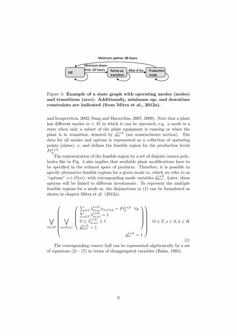
Figure 5: Example of a state graph with operating modes (nodes)and transitions (arcs). Additionally, minimum up- and downtimeconstraints are indicated (from Mitra et al., 2012a).

and Ierapetritou, 2002; Sung and Maravelias, 2007, 2009). Note that a planthas different modes m ∈ M in which it can be operated, e.g. a mode is astate when only a subset of the plant equipment is running or when theplant is in transition, denoted by yt,s,hm (see nomenclature section). Thedata for all modes and options is represented as a collection of operatingpoints (slates), x, and defines the feasible region for the production levelsPrt,s,hg .

The representation of the feasible region by a set of disjoint convex poly-hedra like in Fig. 4 also implies that available plant modifications have tobe specified in the reduced space of products. Therefore, it is possible tospecify alternative feasible regions for a given mode m, which we refer to as“options” o ∈ O(m), with corresponding mode variables yt,s,hm,o . Later, theseoptions will be linked to different investments. To represent the multiplefeasible regions for a mode m, the disjunctions in (1) can be formulated asshown in chapter Mitra et al. (2012a).

∨m∈M

∨

o∈O(m)

∑

i∈I λt,s,hm,o,ixm,o,i,g = Prt,s,hg ∀g∑

i∈I λt,s,hm,o,i = 1

0 ≤ λt,s,hm,o,i ≤ 1

yt,s,hm,o = 1

yt,s,hm = 1

∀t ∈ T, s ∈ S, h ∈ H

(1)The corresponding convex hull can be represented algebraically by a set

of equations (2) - (7) in terms of disaggregated variables (Balas, 1985).

9

∑i∈I

λt,s,hm,o,ixm,o,i,g = Prt,s,hm,o,g ∀m ∈M,o ∈ O(m), g ∈ G, t ∈ T, s ∈ S, h ∈ H (2)∑

i∈Iλt,s,hm,o,i = yt,s,hm,o ∀m ∈M, o ∈ O(m), t ∈ T, s ∈ S, h ∈ H (3)

0 ≤ λt,s,hm,o,i ≤ 1 ∀m ∈M,o ∈ O(m), i ∈ I, t ∈ T, s ∈ S, h ∈ H (4)

Prt,s,hg =∑

m∈M,o∈O(m)

Prt,s,hm,o,g ∀g ∈ G, t ∈ T, s ∈ S, h ∈ H (5)

∑m∈M

yt,s,hm = 1 ∀t ∈ T, s ∈ S, h ∈ H (6)∑o∈O(m)

yt,s,hm,o = yt,s,hm ∀m ∈M, t ∈ T, s ∈ S, h ∈ H (7)

3.2.1.1 Rate of change constraints For transitions between operatingpoints that belong to the same operating mode, the rate of change from hourh to h+ 1 might be restricted. The maximum rate of change in productionof product g (in [mass/∆h]) when operating in mode m (and option o) isdenoted by rm,o,g and calculated according to the same time discretization∆h that is used to calculate the extreme points of the feasible region. Therate of change constraint is written as follows.

|Prt,s,h+1m,o,g − Pr

t,s,hm,o,g| ≤ rm,o,g ∀m ∈M, o ∈ O(m), g ∈ G, t ∈ T, s ∈ S, h ∈ H

(8)

3.2.2 Logic constraints

If the plant switches the mode of operation, logic constraints are required toenforce the feasible transitions that are implied by the state graph, which isshown in Fig. 5. For a detailed derivation of the logic constraints based onpropositional logic (Raman and Grossmann, 1993), we refer to Mitra et al.(2012a, 2012b).

3.2.2.1 Switch variables constraints We introduce binary switchingvariables zt,s,hm,m′ that represent a transition from mode m to m′ in hour h oftime period t and scenario s and link the switching variables with the statevariables yt,s,hm in the following constraint:

∑m′∈M

zt,s,hm′,m−∑m′∈M

zt,s,hm,m′ = yt,s,hm −yt,s,h−1m ∀t ∈ T, s ∈ S, h ∈ H,m ∈M (9)

10

3.2.2.2 Minimum Stay Constraint If the plant needs to stay a min-imum number of hours Km,m′ within a certain mode m′ after a transitionfrom mode m occurred, we can formulate constraint (10). It can be appliedto minimum uptime (after a plant starts up), minimum downtime (after aplant shuts down) and minimum transition time (e.g. during startup proce-dures) constraints.

yt,s,hm′ ≥Kmin

m,m′−1∑θ=0

zt,s,h−θm,m′ ∀(m,m′) ∈MS, ∀t ∈ T, s ∈ S, h ∈ H, (10)

3.2.2.3 Transitional Mode Constraints For the case of a transitionalmode m′, e.g. a startup mode, the plant has to stay Kmin

m,m′ hours withinmode m′ after the transition from mode m (minimum stay, as describedbefore). Afterwards the plant has another transition to mode m′′. Therefore,the two transitions (m to m′ and m′ to m′′) are coupled, which can beexpressed with constraint (11).

zt,s,h−Kmin

m,m′

m,m′ −zt,s,hm′,m′′ = 0 ∀(m,m′,m′′) ∈ Trans,∀t ∈ T, s ∈ S, h ∈ H (11)

The set Trans summarizes all transitions, where a transitional modeconstraint applies.

3.2.2.4 Forbidden Transitions For transitions from mode m to modem′ that are not allowed (summarized in set DAL), the corresponding tran-

sitional variables zt,s,hm,m′ are set to zero, i.e. they do not exist in the model:

zt,s,hm,m′ = 0 ∀(m,m′) ∈ DAL,∀t ∈ T, s ∈ S, h ∈ H (12)

3.2.3 Mass balances and demand satisfaction constraints

Mass balance (13) describes the relationship between current production

levels Prt,s,hg , inventory levels INV t,s,hg and sales St,s,hg for each product g.

If product g cannot be stored (e.g. gas) the upper and lower bounds of theinventory level are zero.

INV t,s,hg + Prt,s,hg = INV t,s,h+1

g + St,s,hg ∀g ∈ G, t ∈ T, s ∈ S, h ∈ H (13)

In constraint (14), the product demand dt,s,hg is met on an hourly level

by either own production or external product purchases, Bt,s,hg , for each

time period t and scenario s. In the particular case of an air separationplant, liquid oxygen and nitrogen are commodity products that can also

11

be shipped from a different plant or be procured from a competitor if theplant is not able to meet demand. The latter case is covered by so-calledproduct-swap agreements that allow to pick up product at a competitor’splant for a pre-set price. On a long-term horizon, shipping product from adifferent plant or product-swap agreements might be attractive in certainhigh-demand scenarios for which it might not be reasonable to expand theplant’s capacity.

St,s,hg +Bt,s,hg ≥ dt,s,hg ∀g ∈ G, t ∈ T, s ∈ S, h ∈ H (14)

3.3 Strategic capacity planning constraints

In the following, we describe the constraints related to strategic capacityplanning decisions: process equipment upgrades, addition of new processequipment and addition of storage tanks.

3.3.1 Process equipment upgrades

We assume that replacing existing equipment does not impact the existenceof the modes the plant initially has. It only changes the polyhedral repre-sentation of the modes that are affected by the equipment upgrade. Hence,the corresponding state variables yt,s,hm,o are linked with binary decisions onupgrades V U tu according to the set Upgrade:

yt,s,hm,o ≤∑

t′∈Tinvest,t′≤tV U t

′u ∀(m, o, u) ∈ Upgrade, t ∈ T, s ∈ S, h ∈ H (15)

In case of an equipment upgrade u that activates option o for mode m,the state variables yt,s,hm,o′ for the other options o′ of mode m, are forced tozero in the current and subsequent time periods.

yt,s,hm,o′ ≤ 1− V U t′u ∀(m, o, u) ∈ Upgrade, o′ ∈ O(m), o′ 6= o,

t ∈ T, t′ ∈ Tinvest, t′ ≤ t, s ∈ S, h ∈ H(16)

Furthermore, we assume that only one equipment upgrade u can be madeover the given time horizon:∑

t∈Tinvest

V U tu ≤ 1 ∀u ∈ U (17)

3.3.2 Addition of new process equipment

If a new equipment n ∈ N is added without removing previously installedequipment, several modes (production and transitional modes) might be

12

introduced. These relations are given by the set NewEq. The state variablesyt,s,hm,o and yt,s,hm are linked with binary decisions on new equipment V N t

n in(18) and (19).

yt,s,hm,o ≤∑

t′∈Tinvest,t′≤tV N t

n ∀(m,n) ∈ NewEq, o ∈ O(m), t ∈ T, s ∈ S, h ∈ H (18)

yt,s,hm ≤∑

t′∈Tinvest,t′≤tV N t

n ∀(m,n) ∈ NewEq, t ∈ T, s ∈ S, h ∈ H (19)

Each investment can be made only once over the given time horizon asper constraint (20). ∑

t∈Tinvest

V N tn ≤ 1 ∀n ∈ N (20)

3.3.3 Addition of product storage tanks

Adding storage capacity of pre-defined size Tankst,g for the final products g,which is indicated by the binary decision variables V Stst,g, does not changethe polyhedral representation of a mode, it only affects the upper bound ofinventory:

INV t,s,hg ≤ INV U

g +∑

st∈ST,t′∈Tinvest,t′≤tTankst,gV S

t′st,g ∀t ∈ T, s ∈ S, h ∈ H, g ∈ G

(21)

3.4 Objective function

The objective function minimizes the total cost TC, which is the sum ofcapital expenses (CAPEXt) and operating expenses (OPEXt,s) across alltime periods t and scenarios s:

TC =∑

t∈Tinvest

CAPEXt +∑

t∈T,s∈Sτ t,sOPEXt,s (22)

3.4.1 Capital expenses (CAPEX)

The capital expenses for time period t ∈ Tinvest are defined by the sumof all investments: new storage tanks (cost coefficient Cstst,g), new processequipment (cost coefficient Cntn) and process equipment upgrades (cost co-efficient Cutu). We assume that all associated cost coefficients are discountedappropriately.

13

CAPEXt =∑

st∈ST,g∈GCstst,gV S

tst,g+

∑n∈N

CntnV Ntn+

∑u∈U

CutuV Utu ∀t ∈ Tinvest

(23)

3.4.2 Operating expenses (OPEX)

The operating expenses for time period t and scenario s consist of fourterms, as shown in equation (24): electricity cost related to production,product procured from competitors, inventory cost and transition cost. It isassumed that the power consumption is known as a linear correlation withthe production levels, where Φm,o,g are the correlation parameters. The costof electricity is given by et,s,h for each season t, scenario s and hour h. Thecost for product procured from a competitor is given by ρt,sg , the cost forinventory holding and the cost for transitions are δg and ζm,m′ respectively.All original cost parameters are multiplied by 13 to match OPEX withCAPEX since we represent one season by a week.

OPEXt,s =∑h∈H

et,s,h(∑

m∈M,o∈O(m),g∈G

Φm,o,gPrt,s,hm,o,g)

+∑g∈G

ρt,sg∑h∈H

Bt,s,hg

+∑g∈G

δg∑h∈H

INVt,s,hg

+∑

m,m′∈Mζm,m′

∑h∈H

zt,s,hm,m′ ∀t ∈ T, s ∈ S

(24)

4 Case Study

One process for which production planning based on time-sensitive pricingcan have significant potential for economic savings is cryogenic air separa-tion, where electricity costs represent 40-50% of overall production costs,which adds $3-5 to the cost of 1 m3 of liquid product. The electricityconsumption is largely due to the high-pressure compression of air that isrequired for the cryogenic separation of its components. Electricity is alsorequired for further compression in order to obtain liquid argon, oxygen andnitrogen.

4.1 Model formulation

In the following, we apply the previously developed modeling framework toan air separation plant, which is illustrated in Fig. 6. The three differ-ent investment options are shown that potentially increase the operational

14

Figure 6: Superstructure of air separation plant with potentialplant modifications: 1. Upgrade existing liquefier (option A) withoption B. 2. Add new liquefier, 3. Add storage tanks for liquidproducts. 1 Simplified scheme.

Figure 7: Operational superstructure in terms of modes: An up-grade of the existing liquefier with “option B”, the polyhedralstructure of mode “existing liquefier” would be replaced. If thesecond liquefier is added, a set of modes is added.

15

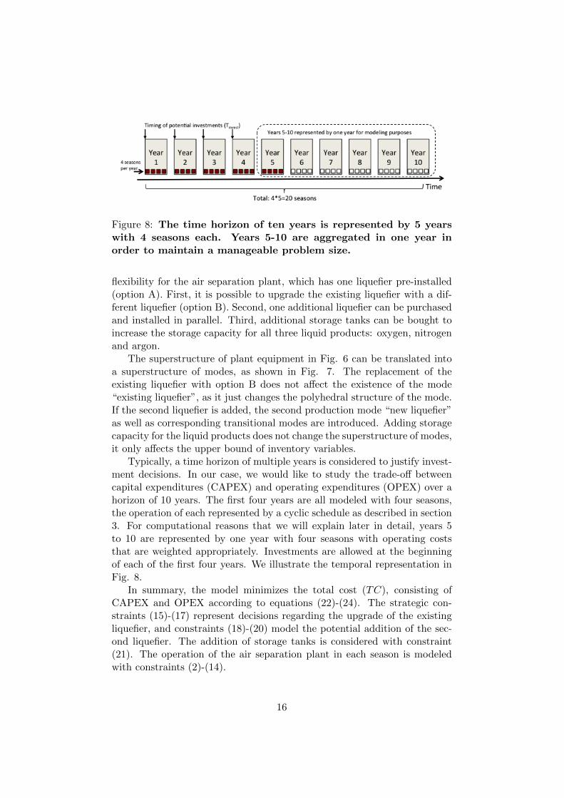
Figure 8: The time horizon of ten years is represented by 5 yearswith 4 seasons each. Years 5-10 are aggregated in one year inorder to maintain a manageable problem size.

flexibility for the air separation plant, which has one liquefier pre-installed(option A). First, it is possible to upgrade the existing liquefier with a dif-ferent liquefier (option B). Second, one additional liquefier can be purchasedand installed in parallel. Third, additional storage tanks can be bought toincrease the storage capacity for all three liquid products: oxygen, nitrogenand argon.

The superstructure of plant equipment in Fig. 6 can be translated intoa superstructure of modes, as shown in Fig. 7. The replacement of theexisting liquefier with option B does not affect the existence of the mode“existing liquefier”, as it just changes the polyhedral structure of the mode.If the second liquefier is added, the second production mode “new liquefier”as well as corresponding transitional modes are introduced. Adding storagecapacity for the liquid products does not change the superstructure of modes,it only affects the upper bound of inventory variables.

Typically, a time horizon of multiple years is considered to justify invest-ment decisions. In our case, we would like to study the trade-off betweencapital expenditures (CAPEX) and operating expenditures (OPEX) over ahorizon of 10 years. The first four years are all modeled with four seasons,the operation of each represented by a cyclic schedule as described in section3. For computational reasons that we will explain later in detail, years 5to 10 are represented by one year with four seasons with operating coststhat are weighted appropriately. Investments are allowed at the beginningof each of the first four years. We illustrate the temporal representation inFig. 8.

In summary, the model minimizes the total cost (TC), consisting ofCAPEX and OPEX according to equations (22)-(24). The strategic con-straints (15)-(17) represent decisions regarding the upgrade of the existingliquefier, and constraints (18)-(20) model the potential addition of the sec-ond liquefier. The addition of storage tanks is considered with constraint(21). The operation of the air separation plant in each season is modeledwith constraints (2)-(14).

16

4.2 Input data

4.2.1 Demand modeling

One of the main drivers, which determines whether an investment shouldbe made or not, is the forecast of the product demand in time period t, Dt,which is a random variable with expected value E(Dt) = µt and associatedstandard deviation σt. As shown in Fig. 9, the annual demand growth ratea, which defines the trajectory of the future demand µt (medium profile), isusually calculated with a regression model that correlates expectations forexternal market factors (e.g. GDP growth) with product demand based onhistorical data. In the following, we refer to the demand of the first year(µ1) as “baseline demand”.

Once the overall demand level is set for a given season, the hourly de-mand dt,s,hg has to be determined. There is a mapping f(µt, σt) → dt,s,hg ,which translates the plant demand into a weekly pattern on an hourly basis.The mapping f is based on historical data. It explains how much product iswithdrawn by the trucks that arrive at the plant during the week, and alsospecifies the ratio of product demands.

In this paper, we investigate the differences in the solutions of the associ-ated optimization problem for two demand models: a deterministic versionand a stochastic model version that addresses the uncertainty in the forecast.

4.2.1.1 Deterministic demand In the deterministic demand model,for each time period t there is just one demand scenario (|S| = 1) withprobability τ t,1 = 1. The demand pattern is based on the expected valueµt. Hence, the demand profile corresponds to the medium demand profilein Fig. 9, and the number of operational subproblems is 4× 5 = 20 due tothe aggregation of years 5-10.

Table 1: Data that characterizes the distributions DI-DIII (seealso Fig. 10), from which demand scenarios are generated forthe stochastic demand model.

Distribution µt σt b τ t,1 τ t,2 τ t,3

(low) (medium) (high)

DI 1 0.065 1.15 25% 50% 25%

DII 1 0.185 1.15 25% 50% 25%

DIII 1 0.23 blow = 1.087 30% 50% 20%bhigh = 1.652

4.2.1.2 Stochastic demand In the stochastic demand model, we ad-ditionally include information that is available regarding the uncertainty in

17

Figure 9: Qualitative illustration of the degrees of freedom in prod-uct demand trajectories and associated scenarios. µt is the ex-pected demand in time period (season) t. σt is the standard devi-ation in time period t. a is the growth rate in demand and blow,bhigh are factors chosen according to the percentile where the lowand high scenarios are centered at.

Figure 10: Distributions DI-DIII and their approximations with 3scenarios that were used in the case study. For DI and DII, thelow and high demand scenarios were centered at the 12.5 and 87.5percentile respectively, and weighted with 25%. The medium sce-nario is weighted with 50%. DI and DII are normal distributions,whereas DIII is skewed.

18

the forecast. First, the distribution of historic demand data is analyzedto determine the underlying distribution. Second, based on the analysis,demand scenarios are generated.

In this paper, we investigate the impact of different demand distribu-tions, such as normal distributions and skewed distributions. Fig. 10 showsthe three distributions DI-DIII, which are used in the case study. All dis-tributions are scaled and centered at 1, as reported in Table 1. DI and DIIare normal distributions, i.e. Dt ∼ N (µt, (σt)2), where 3σtDI ≈ σtDII . DIIIis a skewed distribution with σtDIII > σtDII .

The number of scenarios is limited to three (low, medium, high) pertime period t due to the resulting large size of the optimization problem.Therefore, the number of operational subproblems is 3 × 4 × 5 = 60. Asshown in Fig. 10 and as summarized in Table 1, for DI and DII, the lowand high demand scenarios are centered at the 12.5 and 87.5 percentilerespectively (b = 1.15), and each one is weighted with 25%. The mediumscenario is weighted with 50%, such that

∑s∈S τ

t,s = 1, ∀t. For DIII, thelow demand scenario is closer to the medium demand scenario than the highdemand scenario, since the distribution is skewed. The two different valuesfor b are also reported in Table 1.

4.2.2 Electricity price modeling

The other main influence factor for an investment decision, is electricitycost and in particular the variability in electricity pricing. As mentionedin section 3, the introduction of time periods t, which represent differentseasons of a year, is driven by different typical profiles in electricity prices.We use a weighted average over multiple years of data from PJM (2011) todetermine the baseline price profiles for year one. Based on data publishedby the Energy Information Administration (EIA, 2011), a long-term priceprojection is used to forecast future electricity price levels, while assumingthat the same average pattern will be present in future years as well.

4.2.3 NPV cost modeling

All cost factors in OPEX and CAPEX need to be discounted to consider thetime value of money. We adjust for inflation and use the weighted averagecost of capital (WACC) to discount the cost accordingly.

4.2.4 Summary of the investigated cases

We investigate four cases, in which we vary the baseline demand, the annualgrowth rate, the demand distribution (see section 4.2.1.2) and the price forexternal product purchases. The cases are reported in Table 2. As describedearlier, we solve the cases for deterministic and stochastic demand. In thedeterministic case, the information about the demand distribution is not

19

used. In the stochastic case, the distributions are centered (≡ 1) at thebaseline demand µ1 for year one and at increasing demand values, whichgrow according to the annual growth rate a, for subsequent years.

Table 2: List of investigated cases, for which baseline demand, an-nual growth, the demand distribution and the price for externalpurchases are varied.

case baseline Annual Demand Scaled prices fordemand (µ1) growth (a) distribution external purchases (ρ)

1 65% 3% DI 1.0

2 91% 6.5% DI 1.0

3 81% 4.5% DII 1.0

4 81% 5% DIII 1.33

4.3 Results

4.3.1 Value of current and additional flexibility

For each case, we would like to understand the value of the current flexibility(without new investments) and the value of additional flexibility that can beachieved by retrofitting the air separation plant. Therefore, we investigatethree setups for both, deterministic demand and stochastic demand: (1)constant operation with the currently installed equipment, (2) flexible oper-ation with the currently installed equipment, and (3) the joint optimizationof investment and operational decisions. The difference in total cost between(1) and (2) is the value of the current flexibility. The difference in total costbetween (2) and (3) is the value of additional flexibility. These values maydiffer for the deterministic demand model and the stochastic demand model,which we discuss in the following.

4.3.1.1 Deterministic demand model As one can see in Fig. 11 inwhich total costs are reported for all four cases, the value of current flexibil-ity depends on plant utilization. If utilization is relatively low, as in case 1(65% utilization for the existing liquefier in terms of baseline demand and anannual growth rate of 3%), the plant already has a significant amount of flex-ibility to react to variability in electricity prices with temporary shutdownsand flowrate adjustments during hours of high electricity prices. Therefore,the value of current flexibility is equivalent to a reduction in total costs of13.3% in case 1. In contrast, if the utilization is very high, e.g. in case 2(93% utilization for baseline demand with an annual growth rate of 6%), thevalue of current flexibility to shift production to periods with low electricity

20

Figure 11: Deterministic demand model: Value of current and ad-ditional flexibility. For each case, the value of current flexibilityis the difference between the first two columns; the value of addi-tional flexibility is the difference between the second and the thirdcolumn.

Figure 12: Stochastic demand model: Value of current and addi-tional flexibility. For each case, the value of current flexibility isthe difference between the first two columns; the value of addi-tional flexibility is the difference between the second and the thirdcolumn.

21

prices is low. Hence, the cost savings are relatively small (0.3%). Conse-quently, the value of current flexibility is intermediate if the utilization isalso within a medium range as one can see in cases 3 and 4. Case 3 hasa medium baseline demand of 81% utilization and a growth rate of 4.5%,case 4 has the same baseline demand and a growth rate of 5%. The realizedvalues of current flexibility are equivalent to cost reductions of 2.3% and1.9% respectively.

Only in case 2 investments are made to increase operational flexibility,driven by the higher demand. In the first time period, the second liquefierand an additional storage tank for LN2 are installed. The existing liquefier isnot replaced; neither, additional storage tanks for LO2 or LAr are purchased.The realized cost savings, i.e. the value of additional flexibility, are 7.6%.In all other cases, the joint optimization of investments and operationaldecisions lead to no investments.

4.3.1.2 Stochastic demand model In Fig. 12, the total costs for allcases using the stochastic demand model are reported. As in the determin-istic case, the value of existing flexibility is also a function of utilization.While the absolute total cost values as well as the relative cost savings areslightly different compared to the deterministic solution due to the set ofdemand scenarios, the overall trend is still the same.

In cases 1 and 2, the value of additional flexibility is also similar to thedeterministic solution. While there are no investments made in case 1, thesecond liquefier and one LN2 tank are installed in the first year in case 2,which leads to 7.3% cost savings.

However, in cases 3 and 4, the stochastic solutions suggest a very differentinvestment strategy compared to the deterministic solution. In both cases,the second liquefier and one LN2 tank are installed in the first year. Theassociated values of additional flexibility are 0.5% and 5.9% respectively. Inthe next section, we discuss the origin of the differences and the value of thestochastic solution.

An additional interesting observation is that the investments are alwaysmade during the first time period. Hence, the yearly cost savings due toimproved operational schedules are larger than the potentially lower invest-ment costs due to deferred investments (after inflation and discounting).

4.3.2 Value of the stochastic solution (VSS)

In Fig. 13, one can observe how the additional production capacity of thesecond liquefier increases operational flexibility and allows the plant to ad-just for swings in electricity prices. Furthermore, costs for external productpurchases can be avoided.

In cases 3 and 4, one can observe that the deterministic and the stochas-tic solutions propose different investment strategies. While the deterministic

22

Figure 13: Characteristic operating profiles with and without in-vestments for scenarios at high utilization. Additional productioncapacity of the second liquefier increases operational flexibility andallows the plant to adjust for swings in electricity prices.

23

solutions do not suggest to invest, the stochastic solutions recommend buy-ing the second liquefier and one LN2 tank in the first year. Hence, in Fig.14, we analyze the cost breakdown for the two different investment strategiesunder stochastic demand for cases 3 and 4.

In both cases, the underlying distributions (DII and DIII) have a highstandard deviation from the expected value. Therefore, there are more sce-narios with higher demand that potentially have higher cost due to externalproduct purchases, if no investments are made. Note that the additional liq-uefier provides sufficient production capacity to meet the demand in thesescenarios, such that costs due to external product purchases are practicallyeliminated. Furthermore, the combination of the liquefier with the addi-tional LN2 tanks allows to reduce electricity cost by means of more flexibleproduction schedules. In case 3, the cost difference is 0.5%. In case 4, thecost difference is higher (5.9%) mostly due to the skewed distribution DIII,which generates scenarios with higher deviations from the expected demand,and due to the 33% higher price for external product purchases.

The cost difference we described for cases 3 and 4 is also known as theValue of the Stochastic Solution (VSS). More formally, it can be deter-mined by solving the stochastic version of the problem with the investmentdecisions fixed to the values of the deterministic solution (Birge and Lou-veaux, 2011). If the deterministic and the stochastic solutions suggest thesame investment strategy, the VSS is equal to zero, as in cases 1 and 2.

In Fig. 15, we summarize the drivers behind different investment strate-gies for the deterministic and the stochastic solution with a matrix structure,and classify the investigated cases. Small deviations from the expected de-mand are in favor for similar behavior in both solutions. For cases with lowutilization (low baseline demand and small growth), the deterministic as wellas the stochastic solutions suggest no investments. For cases with high uti-lization (high baseline demand and high growth) both solutions propose newinvestments. However, if the setup is unclear, i.e. if there are large devia-tions from the expected demand, potentially skewed distributions and a highprices for external product purchases, the deterministic and the stochasticsolution behave differently. For those cases, the VSS is greater than zero.

4.3.3 Discussion of computational performance

We solved all test cases within GAMS 23.9.1 (Brooke et al., 2012) on a Inteli7-2600 (3.40 GHz) machine with 8 processors and 8 GB RAM. The com-mercial solver CPLEX 12.4.0.1 was employed using a termination criterionof 0.5% optimality gap. We specified branching priorities on the invest-ment variables V N t

n, V U tu and V Stst,g. Additionally, we used the parallelcomputing capabilities of CPLEX by setting threads=8.

As one can see from Table 3, the problem sizes for the deterministicand the stochastic model are very large due to the multi-scale nature of the

24

Figure 14: Analysis of the value of the stochastic solution (VSS).The flexibility gained from the second liquefier and the additionalLN2 tank reduces electricity cost by means of flexible productionand helps avoiding costs for external product purchases.

Figure 15: Qualitative analysis of VSS (value of stochastic solution)for capacity planning: Stochastic programming helps analyzingunclear demand scenarios.

25

Table 3: Sizes of the resulting optimization problems in terms ofconstraints and variables for the deterministic and the stochasticdemand model.

Deterministic model Stochastic model

Number of 20 60operational problems

Constraints 305,094 915,270

Variables 796,344 2,388,984

Binary Variables 73,940 221,780

optimization problem. In Table 4, we report the computational times andthe corresponding final gaps for deterministic and stochastic demand withthe distinction whether investments are jointly optimized or not.

In 10 out of 16 reported cases, we can converge to the required accuracyof 0.50% final gap. In 5 out of the 6 cases, which do not achieve thataccuracy, the solver runs out of memory, but converges within 1.5% accuracy.Only in one case, the solution process is terminated due to a time limit of80 hours with a final gap of 3.23%. Case 1 is especially difficult to solvebecause the high flexibility leads to a large solution space (3 runs do notconverge to the required accuracy). As expected, the deterministic cases aswell as the cases, in which investments are not optimized, are comparablyeasier to solve due to a smaller solution space.

Since there is a final gap in some cases, it is interesting to understandwhether the obtained solutions are mathematically optimal in terms of in-vestments. In fact, as we will explain in part II of this paper, this questionis one motivating factor for additional research on decomposition methods,which confirms the optimality of the obtained investments for all cases.

5 Conclusion

In this paper, we have described a multi-scale model for the integratedoptimization of investments and operations for continuous power-intensiveprocesses under time-sensitive electricity prices and demand uncertainty. Weapplied the model to an industrial case study of an air separation plant fordeterministic demand as well as stochastic demand.

For different baseline demands, annual growth rates and demand distri-butions, we investigated the current flexibility of the plant and the additionalflexibility due to retrofitting. If the underlying demand distribution has alow standard deviation, the deterministic and the stochastic solution yieldthe same investment strategy. For cases with low utilization, no additionalflexibility needs to be incorporated. For cases with high utilization, the

26

Table 4: Computational times for the investigated cases with flexi-ble operations. Allowed gap: 0.50%. a: out of memory; b: terminatedafter 80 hours of computation

case det./ investments Wall Finalstoch. optimized? time (s) gap (%)

1 det. no 9963 0.50%1 stoch. no 5877 1.25% a

1 det. yes 20128 0.51% a

1 stoch. yes 78810 1.32% a

2 det. no 26 0.09%2 stoch. no 2151 0.38%2 det. yes 1657 0.50%2 stoch. yes 67137 0.50%

3 det. no 37 0.47%3 stoch. no 1190 0.50%3 det. yes 4546 0.50%3 stoch. yes 288000 3.23% b

4 det. no 111 0.46%4 stoch. no 5237 0.55% a

4 det. yes 4814 0.50%4 stoch. yes 154312 0.63% a

27

current flexibility is low and additional flexibility is desirable. However, inunclear demand setups, e.g. medium baseline demand and annual growthrate, with a (potentially skewed) demand distribution that has a large stan-dard deviation, the deterministic and the stochastic solution suggest differ-ent investment strategies. For those case, we showed that the value of thestochastic solution can be significant.

Due to the multi-scale nature of the problem, the resulting MILP prob-lems are large-scale and hard to solve. While most of the investigated prob-lem instances could be solved within at most three days, there is a cleardemand for an efficient algorithm that can solve the problem faster with ahigher numerical accuracy, and can potentially solve instances with a largernumber of scenarios, which would reduce the need for the described aggre-gation of seasons. Therefore, we outline a decomposition algorithm in partII of the paper.

Acknowledgments

We would like to thank Praxair, Inc., and the National Science Foundationfor financial support under grant #1159443.

Nomenclature

Sets

• DAL(m,m′): The set of disallowed transitions from mode m to m′

• G (index g): The set of products. For air separation plants it is{LO2, LN2, LAr, GO2, GN2}.

• H (index h): The set of hours of a week in the operational represen-tation

• I(m, o) (index i), abbreviated as I: The set of extreme points thatrelate to option o of mode m

• M (index m): The set of operating modes

• MS(m,m’) characterizes all minimum stay relationships that hold oncea transition from mode m to mode m′ occurs. Examples include min-imum uptimes, minimum downtimes and minimum transition times.

• N : The set of available new equipment to be added to the plant

• NewEq(m,n), abbreviated as NewEq: The set captures the links be-tween the addition of equipment n with modes m that would be in-troduced to the state graph

28

• O(m) (index o), abbreviated as O: The set of options for mode mdepending on how the plant is modified

• S (index s): The set of demand scenarios

• ST : The set of available storage tanks

• T (index t): The set of time periods related to seasons (four per year);each one’s operation is represented by a cyclic scheduling problem

• Tinvest ⊂ T : The set of time periods, in which investments can takeplace

• Trans(m,m′,m′′): The set of possible transitions from mode m to aproduction mode m′′ with the transitional mode m′ in between

• U : The set of equipment upgrades available

• Upgrade(m, o, u), abbreviated as Upgrade: The set captures the linksbetween the equipment upgrade u and the options o of mode m thatwould be changed in their polyhedral representation

Variables

Binary investment variables

• V U tu: Indicates whether upgrade u is performed in time period t

• V N tn: Describes whether the new equipment n is added in time period

t

• V Stst,g: Indicates whether storage tank st for product g is purchasedin time period t

Binary operational variables

• yt,s,hm : Determines whether the plant operates in mode m in hour h (oftime period t and scenario s)

• yt,s,hm,o : Determines whether the plant operates in option o for mode min hour h (of time period t and scenario s)

• zt,s,hm,m′ : Indicates whether there is a transition from mode m to modem′ from hour h− 1 to h (of time period t and scenario s)

29

Continuous (operational) variables

• Prt,s,hm,o,g: Production amount of product g in option o of mode m in

hour h (of time period t and scenario s)

• Prt,s,hg : Total production of product g in hour h (of time period t andscenario s)

• λt,s,hm,o,i: Variable for the convex combination of slates i to describe thefeasible region of option o of mode m in hour h (of time period t andscenario s)

• INV t,s,hg : Inventory level of product g in hour h (of time period t and

scenario s)

• St,s,hg : Sales of product g in hour h (of time period t and scenario s)

• Bt,s,hg : External product purchases in hour h (of time period t and

scenario s)

• CAPEXt: Capital spent due to investments in time period t

• OPEXt,s: Operating expenses in scenario s of time period t

• TC: Objective function variable that represents total cost

Parameters

• et,s,h: Electricity price in hour h in time period t and scenario s

• Φm,o,g: Coefficient that correlates production level of product g foroption o of mode m with power consumption, in [power/volume]

• ρt,sg : Cost for product g shipped from another plant or procured froma competitor in time period t and scenario s, in [$/volume]

• δg: Cost coefficient for inventory of product g, in [$/volume]

• ζm,m′ : Cost coefficient for transitions from mode m to m′, in [$]

• τ t,s: Probability of scenario s in time period t

• xm,o,i,g: Extreme points of the convex hull of the feasible regions

• Km,m′ : Number of hours the plant has to stay in mode m′ after atransition from mode m

• rm,o,g: Maximum rate of change for product g in option o of mode m

30

• dt,s,hg : Hourly demand for the products g in hour h (in time period tand scenario s).

• INVUg : Current tank capacity for product g

• Tankst,g: Tank size for new storage tank st for product g

• Cstst,g: Cost for purchasing storage tank st for product g in time periodt

• Cntn: Cost for investing in new equipment n in time period t

• Cutu: Cost for investing in the equipment upgrade u in time period t

Other symbols

• Dt: Random variable for the overall product demand in time period t

• µt: The expected demand in time period t, i.e. µt = E(Dt)

• σt: The standard deviation for the demand in time period t

• a: Annual growth rate for product demand

• blow, bhigh: Scaling factors

31

References

[1] Aguilar, O.; Perry, S.J.; Kim, J.-K.; Smith, R. Design and Optimiza-tion of Flexible Utility Systems Subject to Variable Conditions Part1: Modeling Framework. Chemical Engineering Research and Design,85:1136–1148, 2007.

[2] Aguilar, O.; Perry, S.J.; Kim, J.-K.; Smith, R. Design and Optimiza-tion of Flexible Utility Systems Subject to Variable Conditions Part2: Methodology and Applications. Chemical Engineering Research andDesign, 85:1149–1168, 2007.

[3] Balas, E. Disjunctive Programming and a Hierarchy of Relaxationsfor Discrete Optimization Problems. SIAM Journal on Algebraic andDiscrete Methods, 6:466–486, 1985.

[4] Birge, J.R.; Louveaux, F. Introduction to Stochastic Programming.Springer Series in Operations Research. Springer, 2011.

[5] Brooke, A.; Kendrick, D.; Meeraus, A. GAMS: A Users Guide, Release23.9. The Scientific Press, South San Francisco, 2012.

[6] Bruno, J.C.; Fernandez, F.; Castells F.; Grossmann, I.E. MINLP Modelfor Optimal Synthesis and Operation of Utility Plants. Transaction ofthe Institution of Chemical Engineers, 76:246–258, 1998.

[7] Chang, J. Shale Gas is the North American Petrochemical Industry’s“Ace in the Hole”. ICIS Chemical Business, Editors comment, March2010.

[8] Charles River Associates. Primer on Demand-Side Management, Withan Emphasis on Price-responsive Programs, CRA No. D06090. Techni-cal report, The World Bank, 2005.

[9] Chen, Y.; Adams, T.A. II; Barton, P.I. Optimal Design and Operationof Flexible Energy Polygeneration Systems. Industrial & EngineeringChemistry Research, 50:4553–4566, 2011.

[10] Colvin, M.; Maravelias, C.T. A Stochastic Programming Approachfor Clinical Trial Planning in New Drug Development. Computers &Chemical Engineering, 32:2626–2642, 2008.

[11] Conejo, A.J.; Carrion, M.; Morales, J.M. Decision-making under Un-certainty in Electricity Markets. International Series in Operations Re-search and Management Science. Springer, 2010.

[12] Davito, B.; Tai, H.; Uhlaner, R. The Smart Grid and the Promise ofDemand-side Management. McKinsey & Company, 2010.

32

[13] Energy Information Administration. Demand Side Management, An-nual Effects by Program Category. Electric Power Annual, 2009, April2011, 2011.

[14] Goyal, V.; Ierapetritou, M. G. Determination of Operability LimitsUsing Simplicial Approximation. AIChE Journal, 48:2902–2909, 2002.

[15] Grossmann, I.E. Enterprise-wide Optimization: A New Frontier inProcess Systems Engineering. AIChE Journal, 51:1846–1857, 2005.

[16] Grossmann, I.E. Advances in Mathematical Programming Models forEnterprise-wide Optimization. Computers & Chemical Engineering,47:2–18, 2012.

[17] Grossmann, I.E.; C.A. Floudas. Active Constraint Strategy for Flex-ibility Analysis in Chemical Processes. Computers & Chemical Engi-neering, 11:675–693, 1987.

[18] Iyer, R.; Grossmann, I.E. Synthesis and Operational Planning of UtilitySystems for Multiperiod Operation. Computers & Chemical Engineer-ing, 22:979–993, 1998.

[19] Liu, M. L.; Sahinidis, N.V. Optimization in Process Planning underUncertainty. Industrial & Engineering Chemistry Research, 35:4154–4165, 1996.

[20] Liu P.; Pistikopoulos E.N.; Li Z. Decomposition-based Stochastic Pro-gramming Approach for Polygeneration Energy Systems Design underUncertainty. Industrial & Engineering Chemistry Research, 49:3295–3305, 2010.

[21] Maravelias, C.T.; Grossmann, I.E. Simultaneous Planning for NewProduct Development and Batch Manufacturing Facilities. Industrial& Engineering Chemistry Research, 40:6147–6164, 2001.

[22] Mitra, S; Grossmann, I. E.; Pinto, J. M.; Arora, N. Optimal ProductionPlanning under Time-sensitive Electricity Prices for Continuous Power-intensive Processes. Computers & Chemical Engineering, 38:171–184,2012a.

[23] Mitra, S; Sun, L.; Grossmann, I. E. Optimal Scheduling of Indus-trial Combined Heat and Power Plants under Time-sensitive ElectricityPrices. Energy, 2012b. Available online 6 April 2013, ISSN 0360-5442,10.1016/j.energy.2013.02.030.

[24] PJM Interconnection. Daily Day-Ahead Locational Marginal Pricing,2011. http://www.pjm.com.

33

[25] Raman, R.; Grossmann, I.E. Modeling and Computational Techniquesfor Logic Based Integer Programming. Computers & Chemical Engi-neering, 18:563–578, 1993.

[26] Sahinidis, N.V.; Fornari, R.; Grossmann, I.E. Optimization Model forLong Range Planning in the Chemical Industry. Computers & ChemicalEngineering, 13:1049–1063, 1989.

[27] Samad, T.; Kiliccote, S. Smart Grid Technologies and Applications forthe Industrial Sector. Computers & Chemical Engineering, 47:76–84,2012.

[28] Shah, N. Process Industry Supply Chains: Advances and Challenges.Computers & Chemical Engineering, 29:1225–1235, 2005.

[29] Shah, N.; Pantelides, C.C.; Sargent, R. Optimal Periodic Schedulingof Multipurpose Batch Plants. Annals of Operations Research, 42:193–228, 1993.

[30] Sirkin, H.L.; Zinser, M; Hohner, D. Made in America, Again: WhyManufacturing Will Return to the U.S. Boston Consulting Groupstudy., 2011.

[31] Sousa, R.; Shah, N.; Papageorgiou, L.G. Supply Chain Design andMultilevel Planning - An Industrial Case. Computers & Chemical En-gineering, 32:2643–2663, 2008.

[32] Sundaramoorthy, A.; Evans, J. M. B.; Barton, P.I. Capacity Plan-ning under Clinical Trials Uncertainty in Continuous PharmaceuticalManufacturing, 1: Mathematical Framework. Industrial & EngineeringChemistry Research, 51:13692–13702, 2012.

[33] Sung, C.; Maravelias, C. T. An Attainable Region Approach for Effec-tive Production Planning of Multi-product Processes. AIChE Journal,53:1298–1315, 2007.

[34] Sung, C.; Maravelias, C. T. A Projection-Based Method for ProductionPlanning of Multiproduct Facilities. AIChE Journal, 55:2614–2630,2009.

[35] Swaney, R.E.; Grossmann, I.E. An Index for Operational Flexibilityin Chemical Process Design, Part I: Formulation and Theory. AlChEJournal, 31:621–630, 1985.

[36] van den Heever, S. A.; Grossmann, I. E. Disjunctive Multiperiod Op-timization Methods for Design and Planning of Chemical Process Sys-tems. Computers and Chemical Engineering, 23:1075–1095, 1999.

34

[37] Varma, V.A.; Reklaitis, G.V.; Blau, G.; Pekny, J.F. Enterprise-wideModeling & Optimization - An Overview of Emerging Research Chal-lenges and Opportunities. Computers & Chemical Engineering, 31:692–711, 2007.

[38] Voytas, R., Reynolds, J.M., Masiello, J., Pratt, D., Hughes, J.P.,Zarruk, E. et al. Data Collection for Demand-Side Management forQuantifying its Influence on Reliability. Technical report, North Amer-ican Electric Reliability Corporation (NERC), 2007.

[39] You, F.; Grossmann, I.E. Design of Responsive Supply Chains underDemand Uncertainty. Computers & Chemical Engineering, 32:3090–3111, 2008.

35