Optimal Organization: Centralization, Decentralization or

Delegation?

Sergei Severinov∗†

First version: May 15, 1999. This Version: April 2, 2003.

Abstract

The paper addresses the issue of optimal organization of production. I compare three orga-

nizational forms: centralization (one agent produces different inputs), decentralization (each of

two agents produces a different input and contracts directly with the principal), and delegation

(two agents produce different inputs, the principal contracts only with one of them). The key

issue in the comparison of these organizational forms is whether having more information about

costs of production hurts or benefits an agent. I demonstrate that the answer to this question

depends on the degree of substitutability/complementarity between the inputs. I also address

the issue of collusion between agents in the decentralized organization and characterize condi-

tions under which a stake of collusion exists.

JEL Fields: D2, D82, L23

Keywords: organization, incentives, (de)centralization, delegation, collusion,

∗Fuqua School of Business, Duke University, 1 Towerview Drive, Durham, NC 27708, USA, and Department of

Economics, University of Wisconsin-Madison; email:sseverin@duke.edu.†I am grateful to Douglas Bernheim, Peter Hammond, Steve Tadelis, Robert Wilson and seminar participants

at Stanford, University of Pennsylvania, Toronto, Michigan, Vanderbilt, Duke, Wisconsin-Madison for comments

and suggestions. Financial support from Olin Fellowship in Law and Economics and Sloan Foundation is gratefully

acknowledged. All errors are my own.

1 Introduction

One of the central issues in the theory of organizations is how information should be distributed,

exchanged, and processed within an organization. Clearly, providing an answer to this question is

important for the design of optimal organizational structures. The relevant literature has explored

two different approaches to address this issue. The first focuses on the cost of information processing,

while the second studies incentive problems generated by the asymmetry of information between

different parties in an organization.

This paper attempts to contribute to the second strand of literature. It studies an environ-

ment where the principal has to implement a project which requires allocating several tasks to sub-

ordinates (or, alternatively, procuring several inputs from providers) who have private information

regarding the costs of performing these tasks (producing the inputs). The principal has to determine

which organizational structure is optimal and design the contracts with subordinates/providers in

an optimal way. A number of questions naturally arise in this context. Should several tasks (pro-

duction of different inputs) be centralized in the hands of a single agent (supplier), or should those

tasks (production of inputs) be allocated across a number of them? Should the agents be organized

in a hierarchy or not, and should the amount of communication between them be restricted?1

To address these issues, I examine three organizational forms in the context of a production

process requiring two inputs. In a centralized single-agent organization one agent supplies both

inputs. In a decentralized two-agent organization each of the two agents supplies a different input.

Finally, under delegation two agents supply different inputs, but the principal contracts with one

of them and delegates to her the task of contracting with the second agent. The crucial difference

between these organizational forms lies in their informational structure. In the single-agent organi-

zation, the agent has private information about production costs of both inputs, in the two-agent

mechanism each agent knows only the cost of one input, while in the delegated mechanism the

primary contractor serves as an informational intermediary passing the subcontractor’s cost infor-

mation to the principal. Consequently, the relative profitability of these mechanisms depends on the

interaction between these two pieces of information.

Intuitively, the value of information to the agent(s) might be either subadditive or super-

1For example, a city council can hire a single contractor for a municipal project, split the work between several

firms, or allow the primary contractor to subcontract some of the work to others. A firm may train its employees as

specialists in a certain type of tasks, so that several employees typically work on a project. Alternatively, employees

may be trained as generalists who can perform different types of tasks and handle all the work on some projects.

Similar issues arise in a variety of other contexts, including procurement, outsourcing, and regulation. Particularly,

while developing a new defense system, the DoD may decide to procure its components from the same manufacturer

or from different ones. Similarly, the government may allow the existence of a multi-product monopoly, or break it

up into several firms, as in the AT&T case. In more recent examples of deregulation in the electric power industry,

the regulators are called to determine whether a public utility producing the bulk of power could also maintain the

control over the transmission grid, or the latter should be under control of a separate entity.

1

additive. In the subadditive case, the value of using two pieces of information together, as in the

single-agent and delegated mechanisms, is lower than the sum of the values of each piece of informa-

tion used independently, as in the two agent mechanism. In the superadditive case, the ordering goes

in the opposite way.2 Since the principal’s interests are opposite to the agent(s)’ interests, the princi-

pal prefers informational centralization if the value of information is subadditive, and informational

decentralization if the value of information is superadditive.

The main insight of this paper is that the degree of complementarity or substitutability

between the inputs determines whether the value of information is sub- or superadditive. Precisely,

under complementary or small degree of substitutability (to be defined below), the value of infor-

mation is typically (i.e. in the absence of large asymmetries between the two inputs) subadditive,

and it is superadditive when the degree of substitutability is sufficiently large.

To understand why this is so, consider the value of information in a single-agent mechanism.

When the cost of an input is low, the agent earns a rent on this information. The value of this rent

is equal to the surplus obtained by misrepresenting this cost as high, and is therefore proportional

to the quantity of this input delivered under high cost.

Now consider the effect of misrepresenting a low cost of one input on the value of information

about the second input. First, simple incentive compatibility implies that the quantity of the first

input must be decreasing in its cost. Second, the optimal quantity of the second input may be

increasing in the quantity of the first input uniformly in the cost of the second input, as under

complementarity, or decreasing in it, as under substitutability. So, in the first case, misrepresenting

the cost of one input causes the quantity of the second input to go down, and the associated

informational rent to decrease. In the second case, it has the opposite effect.

Thus, the reported cost of one input affects the value of information about the other. We

will refer to this as an ‘internalization factor,’ because a single agent internalizes this effect on

her total payoff. In contrast, in the two-agent mechanism each agent exploits the value of her

information independently taking the other agent’s cost as given, and this effect is not internalized.3

Therefore, under complementarity (substitutability) ‘internalization’ factor tends to make the value

of information subadditive (superadditive).

The comparison between the single-agent and two-agent mechanisms is also affected by an-

other factor - the difference in the structure of incentive constraints. In the single-agent mechanism,

the agent can manipulate both pieces of information, i.e. she can misrepresent production costs of

both goods at the same time. So, a larger set of incentive constraints has to be satisfied there. We2Put otherwise, the main issue is whether from an agent’s point of view the knowledge of another piece of informa-

tion increases the value of the first piece of information or decreases it. In economic literature one can find examples

of situations where more information either unambiguously hurts or benefits the informed party. For example, in

Stackelberg oligopoly game information about a competitor’s action - i.e. her quantity choice- hurts a firm.3This intuition is similar to one explaining why a firm earns more profits in Cournot competition than in Stackelberg

competition where it learns the competitor’s quantity before making its own quantity choice.

2

refer to this as an ‘extra deviation factor.’ This factor makes each piece of information more valuable

when the second piece is also known. So it tends to make information superadditive.

To summarize, whether the value of information is sub- or superadditive and hence which

organizational structure is optimal depends on the relative strength of the ‘internalization’ and the

‘extra deviation’ factors. The single-agent mechanism dominates the two-agent one under comple-

mentarity, because the ‘internalization’ factor favoring a single-agent mechanism is especially potent

in this case. The principal is also able to leverage the effect of the ‘internalization factor’ under sepa-

rability and small degrees of substitutability, and design a mechanism where the value of information

is subadditive. In this mechanism the optimal quantity of one input is increasing in the quantity of

the other input, so the efficient ordering is reversed. But since the degree of substitutability is low,

the associated efficiency losses are small. So, the single-agent mechanism is also optimal in this case.

Nevertheless, the ‘extra deviation’ factor can overturn these results even under complemen-

tarity when there is a strong asymmetry between inputs, i.e. when the marginal product of one

input decreases much more rapidly than the marginal product of the other input and the probability

distributions of input costs are also asymmetric. In this case, it becomes very attractive for a single

agent to make a ‘horizontal’ deviation and misrepresent a combination of low and high cost as high

and low respectively. We show by example (see Proposition 2) that this ‘extra deviation’ factor can

make the two-agent mechanism optimal.

Further, when the degree of substitutability is sufficiently large, it becomes too costly in

terms of efficiency losses to design a mechanism where the quantity of one input increases in the

quantity of the other input. But under reverse ordering the value of information in the single-agent

mechanism becomes superadditive because of the ‘extra deviation’ factor: a low-cost producer of

both inputs can obtain most surplus by misrepresenting both input costs as high. This ‘coordinated’

deviation is infeasible in the two-agent mechanism, so the two agent mechanism is optimal.

Another interesting set of issues arises in the context of delegation. A delegation mechanism

cannot be more profitable than the two-agent mechanism, and the two are equivalent if the primary

contractor could not exploit her position of an informational intermediary to increase her surplus.

Thus, the key issue is whether the primary contractor benefits from intermediating the subcontrac-

tor’s cost information or simply passes it on to the principal. Potentially, she could benefit from

this role in two ways. First, she could try to appropriate some of the subcontractor’s informational

rents. Second, she could manipulate the report regarding the subcontractor’s type to increase the

rent on her own information.

We consider four delegation structures which differ in the extent of the principal’s contractual

abilities. Although the exact conditions under which the two-agent and delegation mechanism are

equivalent vary with the contractual framework, the main conclusion remains the same. The primary

contractor benefits from her role of an informational intermediary if the quantity of one input has

a significant effect on the marginal product of the other input, i.e. if the degree of complementarity

3

or substitutability between the inputs is sufficiently large. This result is easy to understand. Under

these conditions, the quantity of the input produced by the primary contractor and hence her

informational rent are sensitive to the subcontractor’s information. Hence, the primary contractor

has stronger incentives to manipulate the latter.

The issues of incentives within organizations and optimal organizational structure have been

studied by Baron and Besanko (1992), Dana (1993), Gilbert and Riordan (1994), Jansen (1997),

Melumad, Mookherjee and Riechelstein (1995), Laffont and Martimort (1997), (1998), Da Rocha

and de Frutos (1999) and Mookherjee and Tsumagari (2003). Dana (1993) considers the effect of

correlation in the cost structure on the choice between single-agent and two-agent mechanisms under

separability of the production function in the two inputs. He shows that the two-agent mechanism

is optimal when correlation is sufficiently strong, so that the firm can exploit relative performance

evaluation. ‘Informational economies of scope’ discussed by Dana are similar to the effect of ‘internal-

ization factor’ under separability. In contrast, this paper focuses on technological interdependency

and its effect on the relative strength of ‘internalization’ and ‘extra deviation’ factors. There is

no counterpart to our ‘extra deviation’ factor in Dana. Several authors have studied the issue of

optimal organization under perfect complementarity between the inputs. Baron and Besanko (1992)

and Gilbert and Riordan (1994) show that a single-agent mechanism is superior, and the optimal

mechanism can also be implemented via delegation. However, Jansen (1997) demonstrates that the

two-agent mechanism becomes more profitable in the absence of limited liability.4

Perfect complementarity and separability are interesting but quite special cases. Gilbert

and Riordan (1994) point out that their analysis ‘...depends on the fixed proportions production

technology. This is perhaps questionable even in the electricity example, because optimizing the

transmission grid may reduce the need for the new generation capacity...’ i.e. the quality of the grid

and the power output appear to be substitutes. On the other hand, a higher quality of the grid means

a higher stability of the network and a lower probability of outages. This may allow consumers to

substitute out of other forms of energy in favor of electricity. So, the same two inputs may be com-

plements. Other examples with some degree of complementarity or substitutability include express

and regular mail, long distance and local telephony, internet and telephone communication, defense

systems or municipal projects with multiple components. Mookherjee and Tsumagari (2003) estab-

lish results similar to our Proposition 1 and 3 in an environment with continuous type distribution

but symmetric homothetic production function. For this reason, a single-agent mechanism always

dominates a two-agent under complementarity in their framework, and the situation giving rise to

our Proposition 2 does not arise. Furthermore, their definition of complements and substitutes is

based on the properties of the optimal contracts, not the parameters of the model as in this paper.4Iossa (1999) studies the optimal regulatory regime in a two-good economy with one-dimensional uncertainty: the

producer(s) have superior information about the demand for one of the goods, but not about the other. She reaches

a different conclusion that the regulator prefers monopoly (duopoly) when the goods are substitutes (complements).

4

Therefore, there is also no counterparts to our Proposition 4.

The comparison of the single-agent and two-agent mechanisms provides additional insights

regarding the potential for collusion in organizations. Laffont and Martimort (1997) and (1998) have

studied this issue in a similar framework under perfect complementarity. They show that potential

for collusion exists only under additional restrictions on contracts, such as anonymity. Our results

allow to explain why a stake of collusion may not exist then: under complementarity the value of

information is typically subadditive, and so the principal prefers informational centralization. At

the same time, our results imply that potential for collusion exists when the inputs are substitutes:

collusion enables the agents to make a coordinated deviation and report that both costs are high

when they are, in fact, low. More generally, we show that a stake of collusion exists when the

two-agent mechanism is more profitable than a single-agent one.

Our analysis of delegation extends the results of Melumad, Mookherjee and Riechelstein

(1995). We demonstrate that their result on the equivalence of the two-agent and hierarchial mech-

anisms under input observability does not hold generally when the set of possible costs is discrete.

The analysis of the single-agent mechanism involves solving a screening problem with two-

dimensional types. By characterizing the optimal two-dimensional mechanism with a simple distri-

bution of types, but with non-separability between the goods/inputs in the objective function, the

paper contributes to the literature on multidimensional mechanism design (see McAfee and McMil-

lan (1988), Armstrong (1996), and Rochet and Chone (1998)). The contribution in this literature

that is most closely related to our analysis is Armstrong and Rochet (1999) who provide a complete

characterization of the optimal mechanism under separability between the goods, but with arbitrary

degree of correlation between the agents’ types.

The rest of the paper is organized as follows. The model is described in section 2. In section

3, I derive the optimal two-agent mechanism and study the single-agent mechanism. In section 4 I

consider the complementarity case. Section 5 deals with the substitutability case. In section 6 the

results are illustrated via a number of examples. Section 7 studies delegation. In section 8 the issue

of collusion is addressed.

2 Model

A central entity, or principal needs to procure two different goods or inputs. The principal’s benefit

is measured by the production/benefit function v(q1, q2), where q1 (q2) is the quantity of the first

(second) input. I assume that v(., .) is increasing in both arguments, twice continuously differentiable,

and concave. The cross-partial derivative v12(., .) has a constant sign over the relevant domain. We

will say that the inputs are complements (substitutes) if v12(., .) ≥ 0 (v12(., .) < 0). To ensure that

the optimal quantities are positive, I impose Inada boundary condition: limq1→0 v1(q1, q2) = ∞,

∀q2 > 0. This condition is dropped when I consider specific examples.

5

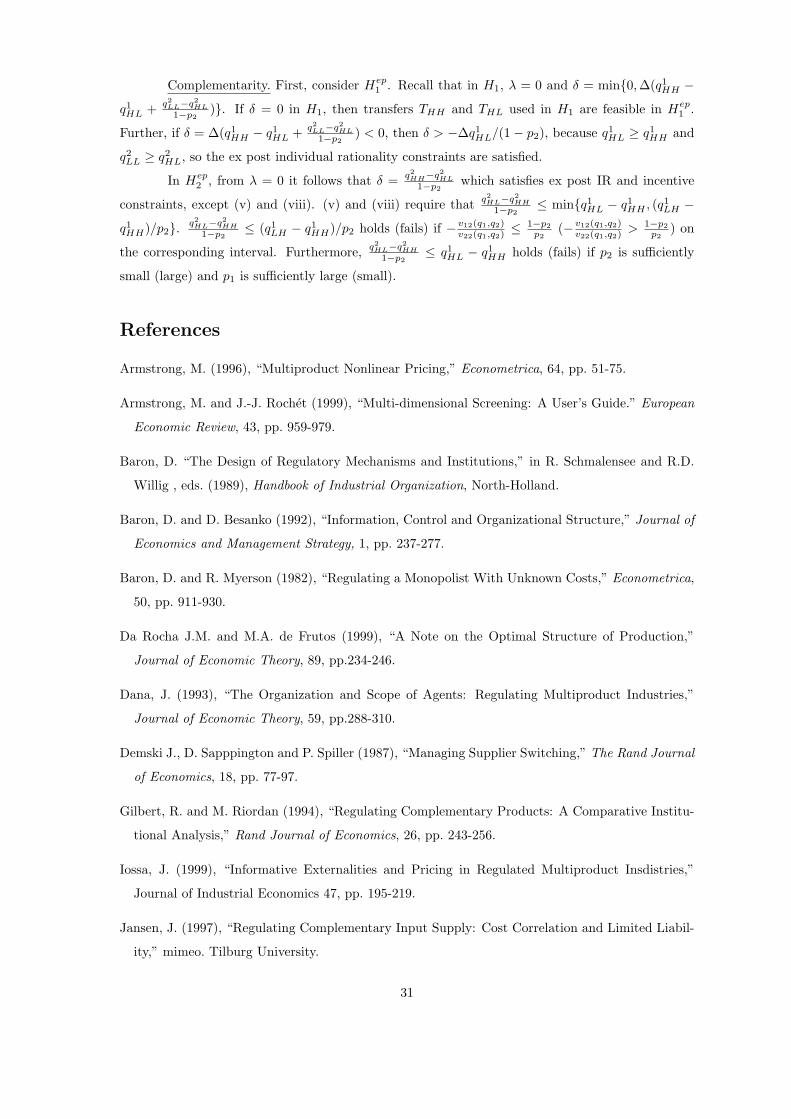
We will compare the performance of the following three organizational forms illustrated in

Figure 1: centralized (one agent produces both inputs), decentralized (each input is produced by

a different agent), or hierarchical delegation (the principal contracts only with the supplier of one

input, who in turn contracts with the supplier of the second input).5

In each organizational form, the principal offers contracts to the agent(s) who may either

accept or reject it. If the contract(s) have been accepted, the agent(s) produce and deliver the goods

(inputs) to the principal and get paid according to the contract(s). Additional stages involving the

contracting between the primary contractor and the subcontractor in the delegation mechanism are

described in section 7.

The principal is risk-neutral, and attempts to maximize her expected benefit net of the

expected payments for the inputs. The agents(s) are risk-neutral and accept the contract after

privately learning their production cost(s). An agent’s reservation utility level is normalized to

zero. An agent cannot produce the good which she is not assigned to. The marginal costs of

production are constant. The levels of production costs are independently distributed across goods

and across agents. Specifically, it is common knowledge that the marginal cost of good i is low (cL)

with probability pi, and is high(cH) with the complementary probability, where cH > cL > 0. Let

∆ = ch−cL. Since production function v(., .) can be arbitrarily asymmetric, the assumption that the

distributions of input costs have a common support is equivalent to a less restrictive ‘common ratio’

assumption c1L

c1H

= c2L

c2H

from which ‘common supports’ can be obtained by simple renormalization of

units. Independence of distributions is assumed in order to abstract from factors on the cost side.

The case of correlated marginal costs is explored in Dana (1993) and Jansen (1997).

Let us now describe the contracts offered by the principal. First, consider single-agent and

two-agent mechanisms. By the Revelation Principle (see e.g. Baron (1989)), we can restrict attention

to direct mechanisms where the agent(s) announce her (their) costs truthfully. A direct mechanism

is a mapping from the set of possible cost types {cL, cH}×{cL, cH} (or states of the world) into the

set of quantities and transfers: R2+×R2 (in the two-agent mechanism), or R2

+×R (in a single-agent

5There is a number of reasons why the principal may want or have to procure all supply of a particular input

from one source. The most common of them is the presence of fixed costs. If large fixed costs in the form of R&D,

investment in equipment, infrastructure and training, etc., have to be sunk by each producer of the good before

she learns her production costs, then having more than one supplier could be prohibitively expensive. Alternatively,

the principal’s commitment to purchase all supply of an input from a particular agent may be required to alleviate

potential hold-up problem and induce this agent to invest.

Consider, for example, the development of a new defense system. In the initial stage of procurement, the government

normally considers bids from a number of firms. However, only one supplier of each major element is ultimately chosen.

Moreover, the final price is usually determined after the contracts have already been awarded. According to Rogerson

(1989), “economies of scale together with very small production runs render it economically infeasible to have two or

more firms build fully functioning production lines... The prices for all production runs may be left to be determined

by future negotiations. Transaction costs together with constantly evolving technological requirements are thought

to render long-term contracts infeasible.”

6

mechanism). The four possible states of the world are denoted by LL, LH,HL and HH. In this

notation, the first (second) letter indicates the marginal cost of the first (second) good.

Let qi = (qiLL, qi

LH , qiHL, qi

HH) denote the vector of quantities of the good i ∈ {1, 2} assigned

in the two-agent mechanism. By convention, the first letter in the subscript refers to the marginal

cost of good i. For example, in the state LH the mechanism assigns quantities q1LH and q2

HL.

Similarly, gi = (giLL, gi

LH , giHL, gi

HH) denotes the vector of quantities of good i assigned in a single-

agent mechanism. Let tiKJ denote the transfer to the agent who produces good i in the two-agent

mechanism, if she announces cost cK and the other agent announces cost cJ (K, J ∈ {L,H}). A

two-agent mechanism has to satisfy the following incentive and individual rationality constraints:

ICi(L) : (tiLL − cLqiLL)pj + (tLH − cLqi

LH)(1− pj) ≥ (tiHL − cLqiHL)pj + (tHH − cLqi

HH)(1− pj)

ICi(H) : (tiHL − cHqiHL)pj + (tHH − cHqi

HH)(1− pj) ≥ (tiLL − cHqiLL)pj + (tLH − cHqi

LH)(1− pj)

IRi(L) : (tiLL − cLqiLL)pj + (tLH − cLqi

LH)(1− pj) ≥ 0

IRi(H) : (tiHL − cHqiHL)pj + (tHH − cHqi

HH)(1− pj) ≥ 0.

Since the principal and the agents are risk-neutral, Bayesian and dominant strategy mecha-

nisms are equivalent, and so the interim incentive and individual rationality constraints can without

loss of generality be replaced by the corresponding ex-post constraints. (For details, see Mookherjee

and Riechelstein (1992)).

Consider now a single-agent mechanism where the agent produces both goods and can

report any possible cost combination. Let TKJ denote the transfer to the agent who announces

costs (cK , cJ), where K, J ∈ {H,L}. Then, the mechanism has to satisfy the following incentive and

individual rationality constraints for all K, J, U, V ∈ {L,H}:

IC(KJ − UV ) : TKJ − cKg1KJ − cJg2

JK ≥ TUV − cUg1UV − cV g2

V U

IR(KJ) : TKJ − cKg1KJ − cJg2

JK ≥ 0.

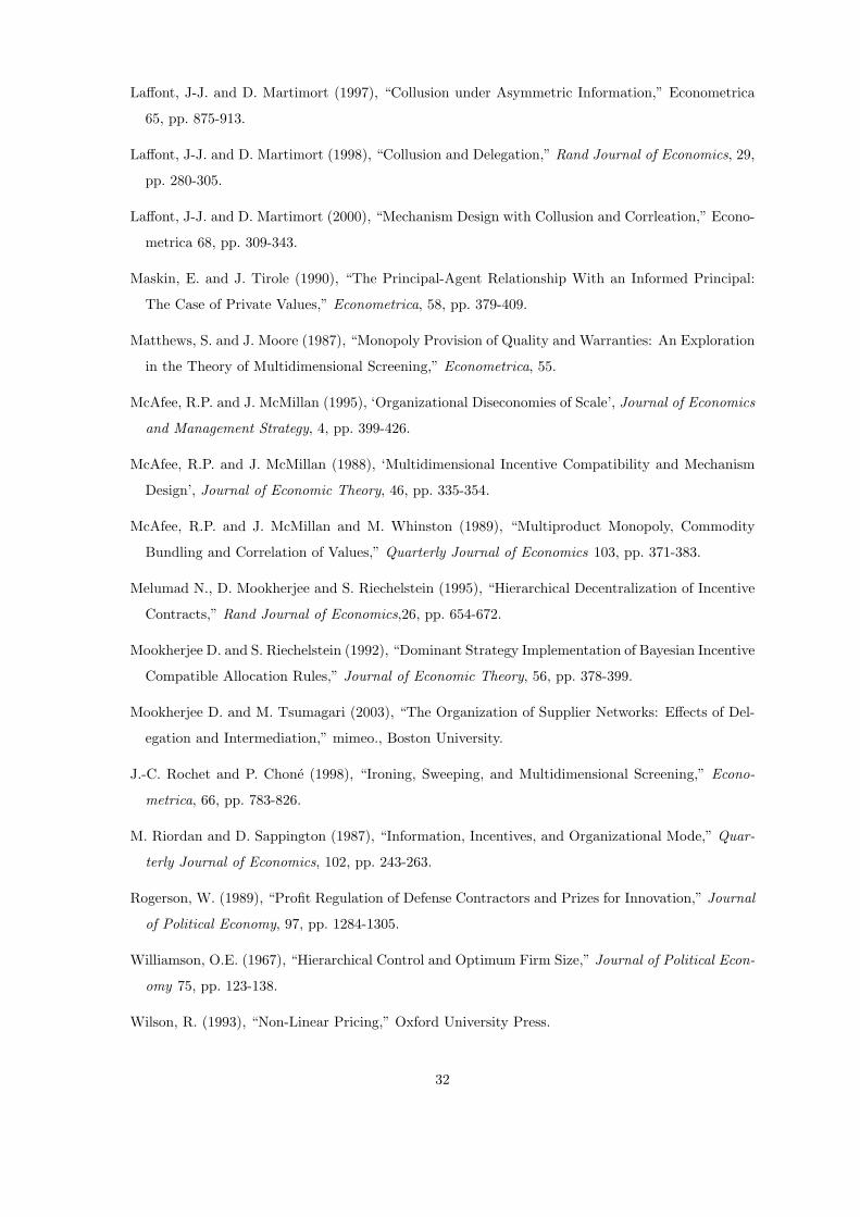
The structures of incentive constraints in the two-agent and single-agent mechanisms are

illustrated in Figure 2. The downward incentive constraint IC(LL−HH), as well as the ‘horizontal’

incentive constraints IC(LH − HL) and IC(HL − LH) in the single-agent mechanism have no

counterparts in a two-agent mechanism, because agents choose their reports independently in the

two-agent mechanism. When any of these constraints are binding, they reduce the profitability of the

single-agent mechanism, so the ‘extra deviation’ factor is effective. On the other hand, constraints

IC(LL − HL), IC(LL − LH) and IC(LL − HH) in the single-agent mechanism are mutually

exclusive, and so the principal can ensure that all these three constraints hold by paying the agent

a single informational rent in the state LL. This is a manifestation of the ‘internalization’ factor.

3 Optimal Mechanisms

First, consider the optimal two-agent mechanism. Essentially, it consists of two submechanisms,

one for each agent. In each of them the individual rationality constraint of the high-cost type

7

and the incentive constraint of the low-cost type are binding. Technological interdependence, i.e.

substitutability or complementarity in the production function, causes the optimal quantity assigned

to one agent to depend on the cost type of the other agent, but has no effect on the set of binding

constraints.

Lemma 1 The optimal two-agent mechanism is unique. The optimal quantities are determined by

the following first-order conditions:

v1(q1LL, q2

LL) = v2(q1LL, q2

LL)v1(q1LH , q2

HL) = v2(q1HL, q2

LH) = cL (1)

v1(q1HL, q2

LH)cH + ∆p1

1− p1(2)

v2(q1LH , q2

HL) = cH + ∆p2

1− p2(3)

v1(q1HH , q2

HH) = cH + ∆p1

1− p1(4)

v2(q1HH , q2

HH) = cH + ∆p2

1− p2(5)

If v12 ≥ 0, qiLL > max{qi

LH , qiHL} and min{qi

LH , qiHL} > qi

HH

If v12 ≤ 0, qiLH > max{qi

LL, qiHH} and min{qi

LL, qiHH} > qi

HL

The principal pays the following transfers to the agents: tiHK = cHqiHK , tiLK = cLqi

LK + ∆qiHK for

K ∈ {L,H}. Thus, the sum of the agents’ expected informational rents equals:

EIR(2) = ∆(p1p2(q1

HL + q2HL) + p1(1− p2)q1

HH + (1− p1)p2q2HH

)(6)

Proof: See the Appendix.

To decrease the agents’ informational rents, the principal distorts all quantity allocations in

the two-agent mechanism, except qiLL and qi

LH , downwards relative to the first-best. The quantities

qiLL are set at the first-best level (no distortion ‘at the top’), while qi

LH is set above (below) the

first-best level when the two inputs are substitutes (complements).

The optimal single-agent mechanism will be analyzed separately under complementarity

and substitutability in the following two sections.

4 Complementarity

In this section I compare the profitability of the single-agent and two-agent mechanisms under

complementarity. The following result does not require characterizing the optimal single-agent

mechanism:

Proposition 1 Suppose that the inputs are complementary (v12(., .) ≥ 0). Single-agent mechanism

is more profitable for the principal than a two-agent mechanism if

max{|v12(q1,q2)||v11(q1,q2)| ,

|v12(q1,q2)||v22(q1,q2)|

}≤ 1 ∀q1, q2 ≥ 0.

8

Proof: See the appendix.

Under the stated condition, the value of information is subadditive and the principal can

implement the allocation profile from the optimal two-agent mechanism via a single-agent mechanism

with lower expected informational rent. Specifically, she can pay a lower informational rent in the

state LL and the same informational rents in the states LH and HL. It is relatively straightforward

to see the latter: in states HH, LH and HL the principal could satisfy all incentive constraints by

paying the agent the sum of transfers that she pays in the same state in the two-agent mechanism.

So, consider state LL. Let us show how the ‘internalization’ factor works there. In the

two-agent mechanism each agent can independently misrepresent her cost as high, so the principal

needs to pay total informational rent ∆(q1HL + q2

HL) to the agents. In the single-agent mechanism,

the agent can deviate by misrepresenting her cost of the first good, the second good, or both goods.

The latter deviation is least attractive under complementarity because qiHL > qi

HH . If the agent

misrepresents only the cost of the first good as high, then she earns surplus equal to ∆q1HL on her

information regarding the first good, but her surplus on information regarding the cost of the second

good is now at most ∆q2HH . Similarly, if the agent misrepresent only the cost of the second good,

her surplus is equal to ∆(q2HL + q1

HH). So, the principal needs to pay informational rent equal to

∆ max{q1HL + q2

HH , q1HH + q2

HL} in state LL. Thus, knowledge of both costs hurts the agent. When

she misrepresents the cost of one good, her ability to earn surplus on the other cost is diminished.

In other words, the value of information is subadditive.

The condition stated in the proposition requires that the complementarity effect be not too

large. If we use the ratio v12(.,.)max{|v11(.,.)|,|v22(.,.)|} as a measure of the degree of complementarity, then

the proposition requires the degree of complementarity to be less than 1. This condition ensures that

the allocation profile from the two-agent mechanism satisfies ‘horizontal’ constraints IC(LH −HL)

and IC(HL− LH) in the single-agent mechanism.

However, ‘horizontal’ incentive constraints IC(HL−LH) and IC(LH−HL) become binding

when the degree of complementarity becomes sufficiently large. Then to satisfy these constraints

the principal has to distort the quantity allocations further away from the efficient level, and/or pay

a higher informational rent to the agent. As a result, under certain parameter values the two-agent

mechanism becomes more profitable than a single-agent mechanism. Precisely, we have.

Proposition 2 Consider quadratic benefit function v(q1, q2) = A+a(q1 + q2)− b12 q2

1− b22 q2

2 +dq1q2,

such that the inputs are complementary i.e. d > 0, and b22 > b1b2 − d2 > 0, d ≥ 2b2, p1

1−p1< p2 <

1−p14 . Then the two-agent mechanism is more profitable for the principal.

Proof: See the appendix.

The proof of the Proposition shows that, if the degree of complementarity is sufficiently large

(d > 2b2), then the horizontal constraint IC(HL − LH) is binding in the single-agent mechanism.

This ‘extra deviation’ factor leads to an increase in the agent’s informational rent, and makes

9

the single-agent mechanism less profitable than a two-agent one. Binding ‘horizontal’ incentive

constraint can also cause two-agent mechanism to outperform single-agent mechanism under perfect

complementarity, as shown by Da Rocha and de Frutos (1999). 6

5 Substitutability

Compared to the complementarity case, there are several differences in the nature and the strength

of the ‘internalization’ and ‘extra deviation’ factors under substitutability. First, the ‘extra devia-

tion’ factor now manifests itself through the downward incentive constraint IC(LL−HH) which can

become binding in the optimal single-agent mechanism. In other words, having two pieces of infor-

mation could be beneficial for the agent because she can misrepresent both low costs as high. In this

case ‘internalization’ factor will no longer enhance the profitability of the single-agent mechanism.

To see this, note that under substitutability it is efficient to set giHL < gi

HH for i ∈ {1, 2}. If

the principal assigns an allocation profile obeying this ordering in the single-agent mechanism, then

IC(LL − HH) becomes binding and the agent obtains informational rent ∆(g1HH + g2

HH) in the

state LL. Yet, if the same quantity allocation profile is implemented via a two-agent mechanism,

in state LL the principal has to pay a lower aggregate rent of ∆(g1HL + g2

HL) to the agents. So, the

two-agent will be optimal.

Still, the potential to exploit the ‘internalization’ factor can make it optimal for the principal

to choose an allocation profile satisfying giHL > gi

HH for i ∈ {1, 2}. We are going to show that this

is optimal when the degree of substitutability is small. Then the ‘extra deviation’ factor will not be

effective and the value of information will be subadditive in the single-agent mechanism. However,

this will not directly imply that single-agent mechanism is optimal, because the quantity allocation

profile in the two-agent mechanism will be more efficient, as is satisfies qiHL > qi

HH for i ∈ {1, 2}

(see Lemma 1). Then the optimal organizational form will be determined by the relative strength of

the ‘internalization’ factors and the higher efficiency of the two-agent mechanism. We will use the

‘homotopy’ technique to measure this tradeoff.

The following lemma formalizes this discussion and allows to make an important simpli-

fication in the analysis. Consider relaxed single-agent program RP (1) in which the principal’s

problem is solved subject only to the downwards incentive constraints IC(LL−LH), IC(LL−HL),

IC(LL−HH), IC(LH−HH), and IC(HL−HH), and individual rationality constraint IR(HH).6Da Rocha and de Frutos (1999) emphasize the asymmetry of the supports of the cost distributions as an explana-

tion of this result. Yet, the complementarity of the production function also plays a crucial role. Indeed, as explained

above, all the results of our paper hold if we replace common support assumption with the ‘common ratio’ assumptionc1Lc1

H

=c2Lc2

H

. Then, by Proposition 1 for any value ofc1H−c1Lc2

H−c2

L

single-agent mechanism remains optimal when the degree

of complementarity is sufficiently small. Under separability, single-agent mechanism is optimal for an arbitrary value

of this ratio. Conversely, it is easy to check that the result of Da Rocha and de Frutos (1999) holds under ‘common

ratio’ assumption, so it also holds in our ‘common support’ case with benefit function v(q1, q2) = min{ q1r1

, q2r2

} when

r1r2

is large enough.

10

Lemma 2 Under substitutability, Relaxed program RP (1) has a unique solution which has the fol-

lowing properties. IR(HH) is binding, and the agent earns informational rent ∆g1HH in state LH,

∆g2HH in state HL, and ∆ max

{g1

HL + g2HH , g1

HH + g2HL, g1

HH + g2HH

}in state LL. The optimal

quantity allocation is characterized by the following first-order conditions for some α ≥ 0 and γ ≥ 0

s.t. α + γ ≤ 1:

v1(g1LL, g2

LL) = v2(g1LL, g2

LL)v1(g1LH , g2

HL) = v2(g1HL, g2

LH) = cL (7)

v1(g1HL, g2

LH) = cH + ∆p1

1− p1α (8)

v2(g1LH , g2

HL) = cH + ∆p2

1− p2γ (9)

v1(g1HH , g2

HH) = cH + ∆p1

1− p1

1− αp2

1− p2(10)

v2(g1HH , g2

HH) = cH + ∆p2

1− p2

1− γp1

1− p1(11)

If the solution to the relaxed program is such that giHL > gi

HH for i ∈ {1, 2} then α + γ = 1,

and the solution to the relaxed program is the optimal single-agent mechanism. α > 0 (γ > 0) only

if g1HL + g2

HH ≥ (≤)g1HH + g2

HL.

If giHH ≥ gi

HL for some i ∈ {1, 2}, then the two-agent mechanism is optimal.

Proof: See the appendix.

Lemma 2 implies that, instead of deriving the optimal single-agent mechanism, it is sufficient

to consider the solution to RP (1). Specifically, we can adopt the following strategy to find the optimal

organizational form. At first, solve RP (1) and check whether giHH ≥ gi

HL for some i ∈ {1, 2}, i.e.

whether IC(LL−HH) is binding. If this is so, then the two-agent mechanism dominates. On the

other hand, if giHL > gi

HH for both i ∈ {1, 2}, then the solution to RP (1) is the optimal single-agent

mechanism, and its profitability has to be compared with that of the optimal two-agent mechanism.

The result of this analysis and hence the optimal organizational form depend on the degree

of substitutability. The latter will be measured by the ratios v12(g1,g2)v11(g1,g2)

and v12(g1,g2)v22(g1,g2)

. These ratios

provide an appropriate measure of the degree of substitutability because they determine how the

optimal quantity of one input changes in response to a change in the quantity of the other input.

Our results can be described as follows. Single-agent (two-agent) mechanism is optimal

when the degree of substitutability is small (large). Additionally, the higher is the probability that

at least one input is produced at high cost, the lower is the threshold degree of substitutability

required for the two-agent mechanism to be optimal. The latter result holds because, when either

p1 or p2 is low, the firm incurs high efficiency losses if it attempts to exploit the ‘internalization’

factor and set giHL > gi

HH . In the remainder of this section we will establish these results formally.

At first, let us focus on the conditions under which the two-agent mechanism is optimal. Let

g1, g2 solve v1(g1

, g2) = cH +∆ p1(1−p1)(1−p2)

and v2(g1, g2) = cL. Also, let g1, g2

solve v1(g1, g2) = cL

and v2(g1, g2) = cH + ∆ p2

(1−p1)(1−p2). Then we have:

11

Proposition 3 Two-agent mechanism is optimal if for all α ∈ (0, 1) either (i) v12(g1,g2)v11(g1,g2)

≥ p2α(1−p2)+(1−α)p1p2

∀g1 ∈ [g1, g1], g2 ∈ [g

2, g2]; or (ii) v12(g1,g2)

v22(g1,g2)≥ p1(1−α)

(1−p1)+αp1p2∀g1 ∈ [g

1, g1], g2 ∈ [g

2, g2].

Proof: See the appendix.

Corollary 1 For all p1, p2 < 1, there exists r < 1 s.t. two-agent mechanism is optimal if

min{ v12(g1,g2)v11(g1,g2)

, v12(g1,g2)v22(g1,g2)

} ≥ r for all g1 ∈ [g1, g1], g2 ∈ [g

2, g2]

Proof: Combining (i) and (ii) in Proposition 3 we obtain that for any p1, p2 < 1:

p2α

(1− p2) + (1− α)p1p2

p1(1− α)(1− p1) + αp1p2

=α(1− α)p1p2

(1− p1)(1− p2) + p1p2(1− (1− α)p1)(1− αp2)< 1

So, for all α ∈ [0, 1] the right-hand side of either (i) or (ii) is less than 1. Q.E.D.

Corollary 2 Suppose that there exist k1 > 0, k2 > 0 and r > 0 s.t. for some i ∈ {1, 2} v12(g1,g2)vii(g1,g2)

≥ r

∀g1 ∈ [l1, l1], g2 ∈ [l2, l2] where l1, l2 satisfy v1(l1, l2) = cH + ∆k1, v2(l1, l2) = cL, and l1, l2 satisfy

v1(l1, l2) = cL, v2(l1, l2) = cH + ∆k2.

Then the two-agent mechanism is optimal if pi < r1+r .

Proposition 3 and its Corollaries show that the two-agent mechanism is optimal when the

degree of substitutability between the inputs is sufficiently large, and it is likely that at least one

input is produced at a high cost. To understand the latter result, note that the ‘internalization’

factor is more powerful when the state LL where this factor applies is more likely, i.e. when both

p1 and p2 are high. Therefore, the threshold degree of substitutability is increasing in p1 and p2.

Obviously, the single-agent mechanism would be optimal under the opposite conditions: a

low degree of substitutability and a high likelihood that both goods are produced at a low cost.

Following the strategy outlined in the discussion of Lemma 2, we show that under these conditions

giHL > gi

HH for i ∈ {1, 2} in the optimal single-agent mechanism. Then we directly compare

the principal’s profits in the optimal single-agent and two-agent mechanisms using the homotopy

technique developed in the appendix.7 The results are stated in the following Proposition.

Proposition 4 Suppose that v12(q1, q2) ≤ 0 for all q1, q2 > 0, and there exist K and K s.t.

K < v11(q1, q2)/v22(q1, q2) < K for all q1 ∈ [q1, q1] and q2 ∈ [q

2, q2]. Then for all p1, p2 ∈ (0, 1)

there exists ω(p1, p2) > 0 increasing in p1, p2 such that the single-agent mechanism is optimal if

max{

v12(q1,q2)v11(q1,q2)

, v12(q1,q2)v22(q1,q2)

}< ω(p1, p2) for all q1 ∈ [q

1, q1] and q2 ∈ [q

2, q2].

Proof: See the appendix.

Thus, when the degree of substitutability is small and/or both p1 and p2 are sufficiently high,

the effect of the ‘internalization’ factor outweighs the efficiency losses from distorting the quantity

allocation profile and setting giHL > gi

HH for i ∈ {1, 2} in the single-agent mechanism.7A simple method of proof based on the comparison of the informational rents is no longer applicable here, because

the optimal quantities are ordered differently in the single-agent and two-agent mechanisms.

12

6 Examples

The following examples illustrate our results. When specific functional forms are considered, suffi-

cient conditions of Propositions 1-4 often translate into simple restrictions on the parameters.

Example 1. Constant Elasticity of Substitution: v(q1, q2) = (α1qρ1 + α2q

ρ2)

mρ where

ρ < 1, 0 < m < 1. Note that the inputs are substitutes (complements) if ρ > m (ρ < m), andv12(q1,q2)vii(q1,q2)

= ρ−m

(1−m)qjqi

+(1−ρ)αiαj

(qjqi

)1−ρ where i, j ∈ {1, 2}.

When q1, q2 satisfy vi(q1, q2) = ci for i ∈ {1, 2} and ci ∈ [cL, cH + pi

(1−pi)(1−pj)], we have:

q1q2

=(

c2α1c1α2

) 11−ρ

, and so v12(q1,q2)vii(q1,q2)

= ρ−m

(1−m)(ciαj/cjαi)1

1−ρ +(1−ρ)cicj

.

Under complementarity (ρ < m), −v12(q1,q2)vii(q1,q2)

< 1 uniformly over R2+ if |m− ρ| is sufficiently

small. In this case, by Proposition 1 the single-agent mechanism is optimal.

Under substitutability (ρ > m), Propositions 3 and 4 imply that the two-agent mechanism

is optimal if ρ − m is large enough, or p1 and p2 are small, while the single-agent mechanism is

optimal if ρ−m is sufficiently small, and p1, p2 are sufficiently large.

Example 2. Quadratic: v(q1, q2) = A + a(q1 + q2)− b12 q2

1 − b2q

2

2+ dq1q2, where a, bi > 0,

d2 < b1b2. In the substitutability case (d < 0), by Proposition 3 the two-agent mechanism is optimal

if −dbi

> pi

1−pifor some i ∈ {1, 2}. By Proposition 4, the single-agent mechanism is optimal if both

−db1

and −db2

are small, and p1 and p2 are sufficiently large.

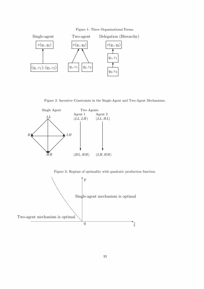
In the complementarity case (d > 0), by Proposition 1 the single-agent mechanism is optimal

if d ≤ min{b1, b2}. However, the two-agent mechanism is optimal under the conditions stated

in Proposition 2. Figure 3 illustrates the regions of optimality of the two-agent and single-agent

mechanisms in the symmetric case where b1 = b2 = b .

We can also use this example to illustrate possible corner solutions which so far have been

ruled out by the Inada conditions. Suppose b1 = b2 = b and p1 = p2 = p and consider the optimal

single-agent mechanism. Then under complementarity gHL > gHH = 0 if cH +∆(

p1−p + p2

2(1−p)2

)<

d < cL + bb−c∆

(1 + p

2(1−p)

). Under substitutability, gHH > gHL = 0 if cL + b

b−c∆ < d < cH +

∆(

p1−p + p2

2(1−p)2

).

Under complementarity, the first-order conditions in Lemmas 1 and 2 can be used to show

that the set of parameter values under which gHL > gHH = 0 is strictly larger than the set of

parameters under which qHL > qHH = 0 in the two-agent mechanism. This observation is interesting

in the context of a more general result due to Armstrong (1996) (see also Rochet and Chone (1998))

establishing the non-emptiness of the set of types who do not trade is the optimal non-linear pricing

mechanism with multidimensional types.

Our observation that in a single-agent mechanism under substitutability gHH > gHL = 0 for

some parameter values, suggests that with a continuous type distribution the set of types who are

assigned zero quantity of at least one good could be disconnected and need not include the origin.

Example 3. Perfect Substitutes: v(q1 + q2). In this case, v12(q1,q2)v11(q1,q2)

≡ 1. Therefore, by

13

Proposition 3 the two-agent mechanism is optimal.

7 Delegation

In this section I consider another form or organization - delegation, or hierarchy. Specifically,

production is performed by two agents who contribute different inputs, but the principal directly

contracts only with one of them (the primary contractor) and delegates to her the task of contracting

with the other agent (the subcontractor)(see figure 1). Delegation is common in the allocation of

tasks within an organization, in procurement and in construction industry. In large corporations

senior managers usually delegate some supervising authority and responsibilities to middle managers.

Hierarchial delegation with asymmetric information was studied by Melumad, Mookherjee

and Riechelstein (1995), Baron and Besanko (1992), Gilbert and Riordan (1994), and Laffont and

Martimort (1998). This literature points out that the advantages of delegation include an economy

of communication costs achieved by shifting some of the contracting tasks from the principal to

one of the subordinates. On the other hand, delegation leads to a loss of control by the principal

which may negatively effect the incentives within hierarchies. The same point is made by McAfee

and McMillan (1995) in the context of a model where intermediate layers of supervision separate

the principal from the agent engaged in production. Riordan and Sappington (1987) show that the

principal’s decision whether to delegate both stages of the production process to the agent or only

one of them depends on whether the costs at the two stages are positively or negatively correlated.

The goal of this section is to compare the profitability of the delegation mechanism vis-a-

vis the two-agent and the single-agent mechanisms. To focus on the issue of the loss of control in

contracting, we make the same assumptions regarding input observability as in the single-agent and

two-agent cases: we assume that under delegation the principal can monitor the quantity of input

supplied by each agent. We will consider two different contractual set-ups referred to as delegation

hierarchies H1 and H2. The following sequence of moves characterizes hierarchy H1:

1. The principal offers the contract to the primary contractor.

2. The primary contractor decides whether to accept or reject the contract. If she rejects, the game

ends and all players obtain their reservation payoffs. If the primary contractor accepts the contract,

then the game proceeds through the following steps:

3. The primary contractor reports her cost type to the principal.

4. The primary contractor offers a contract to the subcontractor. If the subcontractor rejects it,

then the game ends and all players obtain their reservation payoffs.

5. If the subcontractor accepts, she reports her cost type to the primary contractor, who then reports

it to the principal.

6. Both contractors produces their inputs, the final output is delivered to the principal, and the

transfers take place according to the two contracts.

14

H1 is most profitable for the principal among all delegation structures with the same observ-

ability assumptions, because the principal has the broadest possible contracting abilities there. In

particular, the principal signs a contract with the primary contractor and obtains her cost report be-

fore the latter communicates with the subcontractor. This feature has two important consequences.

First, only the interim, rather than ex post, individual rationality constraints of both agents

need to be satisfied. This distinction is irrelevant for the subcontractor, because her situation falls

into the class of cases for which Mookherjee and Riechelstein (1992) has established the equivalence of

Bayesian and dominant strategy implementation. However, there is a significant difference between

the two types of constraints as far as the primary contractor is concerned. If interim constraints

have to hold, then the principal can structure her contract in such a way that the primary contractor

obtains a negative payoff for one realization of the subcontractor’s cost, and a positive payoff for

a different realization of the subcontractor’s cost. On the other hand, the primary contractor’s ex

post individual rationality constraint has to be satisfied if she can withdraw from the contract after

receiving a report from the subcontractor. We demonstrate below that the former regime makes

eliciting information easier for the principal. So, her profits in the delegation mechanism with interim

IR constraints are higher.

Further, in H1 the primary contractor’s decision whether to report her true cost or not

cannot be contingent on the subcontractor’s cost. This reduces the set of feasible deviations by the

primary contractor, which benefits the principal. To highlight this factor, we consider an alternative

contracting arrangement -hierarchy H2- where the primary contractor does not make a cost report

to the principal before communicating with the subcontractor. Formally, the sequence of steps in

H2 is the same as in H1, except that Step 3 is eliminated, and in Step 5 the primary contractor

reports both costs to the principal.

Thus, H2 allows to save some communication costs. However, the set of feasible deviations

for the primary contractor is larger in H2 because she may decide to misrepresent her cost for one

realization of the subcontractor’s cost, but not for the other realization. As we demonstrate in

Proposition 6, this has real consequences: in some cases, the hierarchy H1 is strictly more profitable

for the principal than the hierarchy H2.

A few comments are in order regarding the choice of the primary contractor. In our model,

agents 1 and 2 can be asymmetric with respect to their cost distribution as well as their marginal

products. Intuitively, we allow one agent to be more productive than the other. As shown below,

the nature of these asymmetries is an important determinant affecting the optimal choice of the

primary contractor. In some cases, a hierarchial mechanism can attain the performance of a two-

agent mechanism only if a certain agent is chosen as a primary contractor. However, the choice of the

primary contractor may be determined by factors outside our model, such as specialized knowledge

about potential suppliers of other inputs. For example, the primary contractor in a construction

15

project has to be well-informed about the market for suppliers of necessary materials and services, as

well as the reputations of different firms in this market. These factors may then require the ‘wrong’

agent (from the technological and cost structure point of view) to be chosen as a primary contractor.

To address this issue, we will always start by considering agent 1 as a primary contractor, and

then explore whether switching the roles could affect the performance of the delegated mechanism.

At first, let us establish some preliminary results. Since agents 1 and 2 are risk-neutral,

the informed principal problem does not arise in contracting between them. So, without loss of

generality, we will suppose that the primary contractor with cost cK , K ∈ {L,H}, reveals her type

to the subcontractor and offers her a menu contract consisting of two quantity/transfer pairs.

It is easy to establish that the two-agent mechanism is at least as profitable for the prin-

cipal as H1 or H2. To see this, fix a quantity schedule {hiLL, hi

LH , hiHL, hi

HH}i=2i=1 in a hierarchial

mechanism where 1 stands for the primary contractor, and 2 stands for the subcontractor, and

let (THH , THL, TLH , TLL) be the vector of transfers from the principal to the primary contractor.

The interim participation constraint of the primary contractor with cost cH can be satisfied only if

(1− p2)THH + p2THL(1− p2) is sufficient to cover the expected production costs in states HH and

HL and the subcontractor’s informational rent ∆h2HH in HL. So, in H1 and H2 we have:

(1− p2)THH + p2THL ≥ (1− p2)cH(h1HH + h2

HH) + p2(cHh1HL + cLh2

LH + ∆h2HH) (12)

Similarly, (1 − p2)TLH + p2TLL must cover: (i) production costs in states LH and LL, (ii) sub-

contractor’s informational rent ∆h2HL in state LL, (iii) primary contractor’s expected informational

rent of at least ∆((1− p2)h1HH + p2h

1HL).8 So, in both H1 and H2 we have:

(1− p2)TLH + p2TLL ≥ (1− p2)(cLh1LH + cHh2

HL + ∆h1HH) + p2(cL(h1

LL + h2LL) + ∆(h2

HL + h1HL)) (13)

Combining (12) and (13), we conclude that the expected informational rent that the principal pays

in either hierarchy H1 or H2 is no less than ∆(p1p2(h1HL +h2

HL)+ p1(1− p2)h1HH)+ (1− p1)p2h

2HH)

which is the same as the expected informational rent paid by the principal in the optimal two-

agent mechanism. Therefore, the principal’s expected cost of implementing a quantity schedule via

delegation is at least as large as via the two-agent mechanism.

So, the principal’s payoff from either H1 and H2 is no greater than her payoff from the two-

agent mechanism. In Propositions 5 and 6 we characterize the conditions under which hierarchies

H1 and H2 attain the same profitability as the two-agent mechanism.

Proposition 5 If agent 1 (2) serves as a primary contractor, then H1 attains the same performance

as the two-agent mechanism if∣∣∣ v12(q1,q2)v11(q1,q2)

∣∣∣ ≤ 11−p2

(∣∣∣ v12(q1,q2)v22(q1,q2)

∣∣∣ ≤ 11−p1

)∀q1, q2 ∈ R2

+. Conversely,

the hierarchy H1 with agent 1 (2) as a primary contractor is strictly less profitable for the principal

if∣∣∣ v12(q1,q2)v11(q1,q2)

∣∣∣ > 11−p2

(∣∣∣ v12(q1,q2)v22(q1,q2)

∣∣∣ > 11−p1

)∀q1, q2 ∈ R2

+.

Under complementarity the principal obtains the same payoff in H1 as in the two-agent

mechanism if either agent can serve as the primary contractor.8Otherwise, (12) implies that the primary contractor can earn a higher expected profit by simply reporting H in

the first stage and then implementing (h1HH , h2

HH) in state LH and (h1HL, h2

LH) in state LL.

16

Under substitutability, H1 is strictly more profitable for the principal than the single-agent

mechanism, if IC(LL−HH) is binding in the latter.

Proof: see the appendix.

Proposition 5 establishes that H1 is equivalent to the two-agent mechanism when the cross-

effects in production are not too large, i.e. the marginal product and hence the optimal quantity of

one input is not too sensitive to the quantity of the other input.

To understand this result, note that (12) and (13) imply that each agent obtains at least

as much surplus from private information regarding her own cost as in the two-agent mechanism.

So, H1 is equivalent to the two-agent mechanism only if the primary contractor cannot exploit her

role as an informational intermediary to earn additional surplus, and passes on the information

from the subcontractor to the principal without manipulating it. Manipulating this information

could be profitable for the primary contractor for two reasons: (a) she could appropriate part of

the informational rents that the principal intends for the subcontractor; (b) she could extract more

surplus from her own information.

In hierarchy H1, option (a) is infeasible because the primary contractor has to report her

cost type before communicating with the subcontractor. Given the primary contractor’s report, the

informational rents on the subcontractor’s information can be appropriated only by the subcontrac-

tor. At the same time, option (b) is feasible. It becomes important when the report regarding the

subcontractor’s cost has a significant effect on the quantity assigned to the primary contractor, which

is exactly when the degree of complementarity or substitutability between the inputs is sufficiently

large.

Specifically, suppose that the inputs are complementary and the principal offers a contract

with (12) and (13) holding as equalities. Consider the following deviation: the primary contractor

misrepresents her low cost as high in the first stage, and then always reports that the subcontractor’s

cost is low. Then, the primary contractor has to pay cHq2LH to the subcontractor, with a net loss

of at least ∆(q2LH − q2

HH). However, the surplus obtained by the primary contractor on information

about her own cost increases from ∆(q1HLp2 + q1

HH(1 − p2)) to ∆q1HL. In the proof of Proposition

5, I show that this increase outweighs the extra payment to the subcontractor when the degree of

complementarity is sufficiently large. This is so because a report that the subcontractor’s cost is low

rather than high causes a larger increase in the quantity supplied by the primary contractor, and

hence in her informational rent, than in the quantity supplied by the subcontractor, and hence the

extra payment to her. But then the original contract is not incentive compatible, and so H1 cannot

attain the same performance as the two-agent mechanism.

Similarly, under substitutability the primary contractor’s informational rent increases in the

subcontractor’s cost. So, the primary contractor has an incentive to exaggerate the subcontractor

cost. The principal can offset this incentive to a certain extent by imposing a penalty on the primary

contractor when the latter reports that both costs are high. Yet, this penalty cannot be too large,

17

because otherwise the primary contractor will misrepresent her own high cost as low. So the incentive

to exaggerate the subcontractor’s cost cannot be mitigated when the degree of substitutability is

large.

Next, consider hierarchy H2. There, the primary contractor has a wider set of possible

deviations, and can try to appropriate some of the subcontractor’s informational rents. In particular,

under complementarity she will have an incentive to misrepresent the state LH as HH in order to

lower the informational rent that she pays to the subcontractor in state LL. Thus, H2 attains the

same performance as the two-agent mechanism under more restrictive conditions than H2.

Proposition 6 If agent 1 (2) serves as a primary contractor, then H2 attains the same performance

as the two-agent mechanism if∣∣∣ v12(q1,q2)v11(q1,q2)

∣∣∣ ≤ 1−p11−p2

(∣∣∣ v12(q1,q2)v22(q1,q2)

∣∣∣ ≤ 1−p21−p1

)∀q1, q2 ∈ R2

+. Conversely,

the hierarchy H2 with agent 1 (2) as a primary contractor is strictly less profitable for the principal

if∣∣∣ v12(q1,q2)v11(q1,q2)

∣∣∣ > 1−p11−p2

(∣∣∣ v12(q1,q2)v22(q1,q2)

∣∣∣ > 1−p21−p1

)∀q1, q2 ∈ R2

+.

If either agent can serve as a primary contractor, then H2 attains the same performance as

the two-agent mechanism if∣∣∣ v12(q1,q2)v11(q1,q2)

∣∣∣ ≤ 11−p2

and∣∣∣ v12(q1,q2)v22(q1,q2)

∣∣∣ ≤ 1−p21−p1

∀q1, q2 ∈ R2+.

Proof: see the appendix.

Finally, let us consider the case where the primary contractor could refuse to deliver the

inputs and opt out of the contract after receiving the subcontractor’s report. Then the individual

rationality constraint of the primary contractor has to hold ex post. Accordingly, let Hep1 (Hep

2 ) be

a modification of hierarchy H1 (H2) obtained by adding agent 1’s option to withdraw immediately

after stage 5. We have:

Proposition 7 Under substitutability, both Hep1 and Hep

2 are strictly less profitable for the principal

than the two-agent mechanism.

Under complementarity, Hep1 attains the same performance as the two-agent mechanism, if

H1 attains this performance. When agent 1 serves as a primary contractor, then Hep2 attains the

same performance as the two-agent mechanism if H2 attains the same performance and, additionally,

−v12(q1,q2)v22(q1,q2)

≤ 1−p2p2

∀q1, q2, p2 is sufficiently small, p1 is large.

In Hep1 and Hep

2 , the principal does not have the ability to distribute the expected payments

to the primary contractor across the states of the world in an arbitrary way. This restricts her ability

to mitigate the primary contractor’s incentives to manipulate the subcontractor’s information, and

so Hep1 and Hep

2 attain the same performance as the two-agent mechanism under more restrictive

conditions than H1 and H2 respectively.

8 Collusion

The results of the previous sections can be used to address the issue of collusion in organizations.

Laffont and Martimort (1997) and Laffont and Martimort (1998)) (LM in the sequel) analyze this

18

issue in a virtually identical framework, and therefore it will be natural to compare our results to

theirs. The potential for collusion arises in the two-agent mechanism if the agents can communicate

and adopt a joint reporting strategy. However, collusion will not necessarily generate additional

payoff for them and hence a loss for the principal. In the terminology of LM, a stake of collusion

may not exist.

Obviously, the agents can achieve the highest joint payoff from collusion if they can overcome

the asymmetric information and bargaining problem between them and act as a single entity. We

call this situation perfect collusion. Clearly, if there is no stake of perfect collusion, then there is also

no stake of collusion which is less than perfect, i.e. when some bargaining frictions exist between

the agents.

When does a stake of perfect collusion exists? We can provide an answer to this question

using the comparison of the single-agent and two-agent mechanisms. Specifically, suppose that the

allocation profile from the optimal two-agent mechanism is assigned in the single-agent mechanism.

Then a stake of collusion exists if such mechanism is not incentive compatible, i.e. in some state(s)

of the world the single agent has an incentive to misrepresent the costs of both inputs which is

not feasible in the two-agent mechanism without collusion. On the contrary, there is no stake of

collusion if the mechanism remains incentive compatible. This observation gives rise to the following

proposition:

Proposition 8 A stake of perfect collusion exists in each of the following two cases:

(i) the two-agent mechanism is more profitable for the principal than the single-agent one,

(ii) under substitutability.

A stake of perfect collusion does not exist when the inputs are complementary and

max{

v12(q1,q2)|v11(q1,q2)

, v12(q1,q2)|v22(q1,q2)|

}≤ 1 ∀q1, q2.

Proof: Suppose that the two-agent mechanism dominates the single-agent one. Let M2 be the

optimal two-agent mechanism with quantities and transfers given by (q1KJ , t1KJ , q2

JK , t2JK) (K, J ∈

{L,H}). Suppose that the principal offers to a single agent a mechanism M1 which assigns the

same quantities as in M2 and transfers equal to the sum of transfers in M2. Formally, giKJ = qi

KJ

∀i, K, J and TKJ = t1KJ + t2JK . M1 cannot be incentive compatible, because otherwise single-agent

mechanism would be at least as profitable as the optimal two-agent mechanism, contradicting our

original assumption. When the two agents collude perfectly, they act as a single agent, and so the

colluding pair will make the same announcements in M2 as a single agent in M1. Thus, M2 is not

incentive compatible under perfect collusion, so a stake of collusion exists.

Under substitutability, the allocation profile in the optimal two-agent mechanism satisfies

qiHH > qi

HL, so the colluding agents would deviate by reporting HH in state LL.

Consider now the complementarity case. Then the allocation profile in the optimal two-

agent mechanism satisfies qiHH > qi

HL. So, if this allocation profile is assigned in a single-agent

19

mechanism, IC(LL − HH) will hold. Furthermore, under the stated condition both ‘horizontal’

constraint will also hold in the single-agent mechanism. Q.E.D.

Since LM focus on the case of perfect complementarity where a stake of collusion does not

exist, they had to impose additional restrictions on the set of feasible mechanisms. Specifically, they

require the principal to offer an anonymous contract so that both agents get the same transfer in

each state of the world. The anonymity generates a stake of collusion proportional to qHL − qHH .

However, this stake of collusion disappears under substitutability and also when the benefit function

is additively separable.

LM (1998) demonstrate that the principal can avoid the cost of preventing collusion in

an anonymous mechanism through delegation. Their delegation mechanism (equivalent to our H2

hierarchy) is more profitable for the principal than a two-agent mechanism with collusion. Yet,

without anonymity restriction this result is not always true. In particular, suppose that inputs

are complementary and agent 1 is a primary contractor. Propositions 6 and 8 imply that if

max{

v12(q1,q2)|v11(q1,q2)

, v12(q1,q2)|v22(q1,q2)|

}≤ 1 and v12(q1,q2)

|v11(q1,q2)| > 1−p11−p2

, then there is no stake of collusion, and

H2 is strictly less profitable than a two-agent mechanism.

9 Appendix

The following easy to prove properties of concave functions will be useful below.

Property 1. Let v(., .) be a twice-continuously differentiable, increasing, concave function. Consider

d, c ∈ (0,∞) s.t. v1(q1, q2) = c and v2(q1, q2) = d. Then dq1dc < 0 and dq2

dc v12 < 0.

Property 2: Suppose that v1(q1, q2) = c1 and v2(q1, q2) = c2 for some c1, c2 > 0. Then:

dq1

dc1≤ dq2

dc1if |v22(q1, q2)| ≥ |v12(q1, q2)| and

dq2

dc2≤ dq2

dc1if |v11(q1, q2)| ≥ |v12(q1, q2)|

Proof of lemma 1: The optimal two-agent mechanism is derived by solving the following problem

subject to the constraints IRi(H) and ICi(L) for i ∈ {1, 2}:

maxq1

JK ,q2JK ,t1KJ ,t2JK , J,K∈{1,2}

p1p2(v(q1LL, q2

LL)− t1LL − t2LL) + p1(1− p2)(v(q1LH , q2

HL)− t1LH − t2HL)+

(1− p1)p2(v(q1HL, q2

LH)− t1HL − t2LH) + (1− p1)(1− p2)(v(q1HH , q2

HH)− t1HH − t2HH)

Since v(., .) is concave, this problem has a unique solution. The quantities are characterized by the

first-order conditions in the lemma. Applying Property 1, we obtain desired ordering. The transfers

are chosen so that IRi(H) and ICi(L) are binding. Since qiLL > qi

HL and qiLH > qi

HH , the incentive

constraint of the high-cost agent is not binding, and the expected informational rent EIR(2) is given

by the expression in the statement of the lemma. QED.

Proof of Proposition 1: Consider the following single-agent mechanism. In state of the world

KJ , assign the same quantity allocation (q1KJ , q2

JK) as in the optimal two-agent mechanism, and

20

the transfer from the following list: THH = cH(q1HH + q2

HH), TLH = cLq1LH + cHq2

HL + ∆q1HH ,

THL = cHq1HL + cLq2

LH + ∆q2HH , TLL = cL(q1

LL + q2LL) + ∆ max{q1

HL + q2HH , q2

HL + q1HH}.

This mechanism is more profitable for the principal than the optimal two-agent mechanism,

because her outlay is the same in all states of the world except LL, in which her outlay is lower

by ∆ min{q1HL − q1

HH , q2HL − q2

HH} > 0 than in the two-agent mechanism. The proposed mech-

anism satisfies all individual rationality constraint. Let us show that this mechanism is incentive

compatible. Clearly, it satisfies all downwards incentive constraints IC(LL −HL), IC(LL − LH),

IC(LL−HH), IC(LH −HH), IC(HL−HH). It is easy to see that all upwards constraints hold.

Now consider the ‘horizontal’ incentive constraints IC(LH−HL) and IC(HL−LH). Since

IC(LH −HH) and IC(HL−HH) are binding, IC(LH −HL) holds if

q2LH − q1

HL ≥ q2HH − q1

HH (14)

Similarly, IC(HL − LH) holds if q1LH − q2

HL ≥ q1HH − q2

HH . To see that (14) holds note that

by (1)-(5), v2(q1HL, q2

LH) < v2(q1HH , q2

HH) and v1(q1HL, q2

LH) = v1(q1HH , q2

HH). Since |v11(q1, q2)| ≥

v12(q1, q2), Property 2, implies that (14) holds. Similarly, the first-order conditions in Lemma 1,

the assumption that |v22(q1, q2)| ≥ v12(q1, q2) and Property 2 imply that IC(HL− LH) holds.

Finally, since IC(LH − HL) and IC(HL − LH) hold and qiLL > qi

LH , it follows that the

upwards constraints IC(HL− LL), IC(LH − LL), and IC(HH − LL) also hold.

Proof of Proposition 2: The proof consists of 3 steps. First, I characterize the optimal single-

agent mechanism. Armstrong and Rochet (1999) solve this problem under separability between the

goods, but for an arbitrary degree of correlation between the types. Second, I derive a method

to compare the profitability of the single-agent and two-agent mechanisms. Third, this method is

applied to show that two-agent mechanism is more profitable for specific functional forms.

Step 1. Consider the firm’s profit maximization problem with the following constraints

imposed explicitly: IR(HH), IC(LL−HL), IC(LL−LH), IC(LL−HH), IC(LH−HH), IC(HL−HH), IC(LH −HL), IC(HL− LH). The Lagrangian associated with this problem is:

maxL = p1p2

(v(g1

LL, g2LL)− TLL

)+ p1(1− p2)

(v(g1

LH , g2HL)− TLH

)+ (1− p1)p2

(v(g1

HL, g2LH)− THL

)+ (1− p1)(1− p2)

(v(g1

HH , g2HH)− THH

)+

λLH

(TLL − cL(g1

LL + g2LL)− TLH + cL(g1

LH + g2HL)

)+ λHL

(TLL − cL(g1

LL + g2LL)− THL + cL(g1

HL + g2LH)

)+

λHH

(TLL − cL(g1

LL + g2LL)− THH + cL(g1

HH + g2HH)

)+ δ1

HH

(TLH − cLg1

LH − cHg2HL − THH + cLg1

HH + cHg2HH

)+ δ2

HH

(THL − cHg1

HL − cLg2LH − THH + cHg1

HH + cLg2HH

)+ µ

(THL − cHg1

HL − cLg2LH − TLH + cHg1

LH + cLg2HL

)+ κ

(TLH − cLg1

LH − cHg2HL − THL + cLg1

HL + cHg2LH

)+ η

(THH − cH(g1

HH + g2HH)

)(15)

21

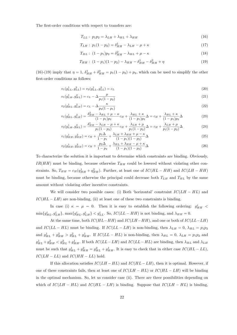
The first-order conditions with respect to transfers are:

TLL : p1p2 = λLH + λHL + λHH (16)

TLH : p1(1− p2) = δ1HH − λLH − µ + κ (17)

THL : (1− p1)p2 = δ2HH − λHL + µ− κ (18)

THH : (1− p1)(1− p2)− λHH − δ1HH − δ2

HH + η (19)

(16)-(19) imply that η = 1, δ1HH + δ2

HH = p1(1− p2) + p2, which can be used to simplify the other

first-order conditions as follows:

v1(g1LL, g2

LL) = v2(g1LL, g2

LL) = cL (20)

v1(g1LH , g2

HL) = cL −∆µ

p1(1− p2)(21)

v2(g1HL, g2

LH) = cL −∆κ

p2(1− p1)(22)

v1(g1HL, g2

LH) =δ2

HH − λHL + µ− κ

(1− p1)p2cH +

λHL + κ

(1− p1)p2∆ = cH +

λHL + κ

(1− p1)p2∆ (23)

v2(g1LH , g2

HL) =δ1

HH − λLH − µ + κ

p1(1− p2)cH +

λLH + µ

p1(1− p2)∆ = cH +

λLH + µ

p1(1− p2)∆ (24)

v1(g1HH , g2

HH) = cH +p1∆

1− p1+

λLH + λHH + µ− κ

(1− p1)(1− p2)∆ (25)

v2(g1HH , g2

HH) = cH +p2∆

1− p2+

λHL + λHH − µ + κ

(1− p1)(1− p2)∆ (26)

To characterize the solution it is important to determine which constraints are binding. Obviously,

IR(HH) must be binding, because otherwise THH could be lowered without violating other con-

straints. So, THH = cH(q1HH + q2

HH). Further, at least one of IC(HL −HH) and IC(LH −HH)

must be binding, because otherwise the principal could decrease both TLH and THL by the same

amount without violating other incentive constraints.

We will consider two possible cases: (i) Both ‘horizontal’ constraint IC(LH − HL) and

IC(HL− LH) are non-binding, (ii) at least one of these two constraints is binding.

In case (i) κ = µ = 0. Then it is easy to establish the following ordering: giHH <

min{giHL, gi

LH}, max{giHL, gi

LH} < giLL. So, IC(LL−HH) is not binding, and λHH = 0.

At the same time, both IC(HL−HH) and IC(LH−HH), and one or both of IC(LL−LH)

and IC(LL −HL) must be binding. If IC(LL − LH) is non-binding, then λLH = 0, λHL = p1p2

and g1HL + g2

HH > g2HL + g1

HH . If IC(LL − HL) is non-binding, then λHL = 0, λLH = p1p2 and

g1HL + g2

HH < g2HL + g1

HH . If both IC(LL−LH) and IC(LL−HL) are binding, then λHL and λLH

must be such that g1HL + g2

HH = g2HL + g1

HH . It is easy to check that in either case IC(HL− LL),

IC(LH − LL) and IC(HH − LL) hold.

If this allocation satisfies IC(LH −HL) and IC(HL−LH), then it is optimal. However, if

one of these constraints fails, then at least one of IC(LH −HL) or IC(HL− LH) will be binding

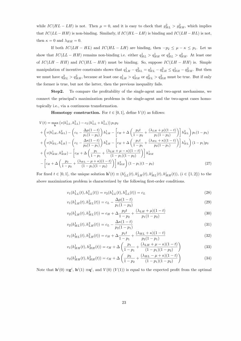
in the optimal mechanism. So, let us consider case (ii). There are three possibilities depending on

which of IC(LH − HL) and IC(HL − LH) is binding. Suppose that IC(LH − HL) is binding,

22

while IC(HL − LH) is not. Then µ = 0, and it is easy to check that g2HL > g2

HH , which implies

that IC(LL−HH) is non-binding. Similarly, if IC(HL−LH) is binding and IC(LH−HL) is not,

then κ = 0 and λHH = 0.

If both IC(LH − HL) and IC(HL − LH) are binding, then −p2 ≤ µ − κ ≤ p1. Let us

show that IC(LL −HH) remains non-binding i.e. either q1HL > q1

HH or q2HL > q2

HH . At least one

of IC(LH − HH) and IC(HL − HH) must be binding. So, suppose IC(LH − HH) is. Simple

manipulation of incentive constraints shows that q1LH − q2

HL = q1HL − q2

LH ≤ q1HH − q2

HH . But then

we must have q2HL > q2

HH , because at least one q1LH > q1

HH or q2HL > q2

HH must be true. But if only

the former is true, but not the latter, then the previous inequality fails.

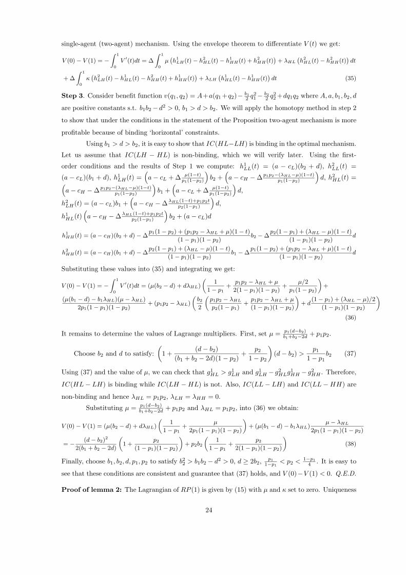
Step2. To compare the profitability of the single-agent and two-agent mechanisms, we

connect the principal’s maximization problems in the single-agent and the two-agent cases homo-

topically i.e., via a continuous transformation.

Homotopy construction. For t ∈ [0, 1], define V (t) as follows:

V (t) = maxh

(v(h1

LL, h2LL)− cL(h1

LL + h2LL)

)p1p2

+

(v(h1

LH , h2HL)−

(cL −

∆µ(1− t)

p1(1− p2)

)h1

LH −[cH + ∆

(p2t

1− p2+

(λLH + µ)(1− t)

p1(1− p2)

)]h2

HL

)p1(1− p2)

+

(v(h1

HL, h2LH)−

(cL −

∆κ(1− t)

p2(1− p1)

)h2

LH −[cH + ∆

(p1t

1− p1+

(λHL + κ)(1− t)

p2(1− p1)

)]h1

HL

)(1− p1)p2

+

(v(h1

HH , h2HH)−

[cH + ∆

(p1

1− p1+

(λLH + µ− κ)(1− t)

(1− p1)(1− p2)

)]h1

HH

−[cH + ∆

(p2

1− p2+

(λHL − µ + κ)(1− t)

(1− p1)(1− p2)

)]h2

HH

)(1− p1)(1− p2) (27)

For fixed t ∈ [0, 1], the unique solution hi(t) ≡ (hiLL(t), hi

LH(t), hiHL(t), hi

HH(t)), (i ∈ {1, 2}) to the

above maximization problem is characterized by the following first-order conditions.

v1(h1LL(t), h2

LL(t)) = v2(h1LL(t), h2

LL(t)) = cL (28)

v1(h1LH(t), h2

HL(t)) = cL −∆µ(1− t)p1(1− p2)

(29)

v2(h1LH(t), h2

HL(t)) = cH + ∆p2t

1− p2+

(λLH + µ)(1− t)p1(1− p2)

(30)

v2(h1HL(t), h2

LH(t)) = cL −∆κ(1− t)p2(1− p1)

(31)

v1(h1HL(t), h2

LH(t)) = cH + ∆p1t

1− p1+

(λHL + κ)(1− t)p2(1− p1)

(32)

v1(h1HH(t), h2

HH(t)) = cH + ∆(

p1

1− p1+

(λLH + µ− κ)(1− t)(1− p1)(1− p2)

)(33)

v2(h1HH(t), h2

HH(t)) = cH + ∆(

p2

1− p2+

(λHL − µ + κ)(1− t)(1− p1)(1− p2)

)(34)

Note that hi(0) ≡gi, hi(1) ≡qi, and V (0) (V (1)) is equal to the expected profit from the optimal

23

single-agent (two-agent) mechanism. Using the envelope theorem to differentiate V (t) we get:

V (0)− V (1) = −∫ 1

0

V ′(t)dt = ∆

∫ 1

0

µ(h1

LH(t)− h2HL(t)− h1

HH(t) + h2HH(t)

)+ λHL

(h2

HL(t)− h2HH(t)

)dt

+ ∆

∫ 1

0

κ(h2

LH(t)− h1HL(t)− h2

HH(t) + h1HH(t)

)+ λLH

(h1

HL(t)− h1HH(t)

)dt (35)

Step 3. Consider benefit function v(q1, q2) = A+a(q1 +q2)− b12 q2

1− b22 q2

2 +dq1q2 where A, a, b1, b2, d

are positive constants s.t. b1b2− d2 > 0, b1 > d > b2. We will apply the homotopy method in step 2

to show that under the conditions in the statement of the Proposition two-agent mechanism is more

profitable because of binding ‘horizontal’ constraints.

Using b1 > d > b2, it is easy to show that IC(HL−LH) is binding in the optimal mechanism.

Let us assume that IC(LH − HL) is non-binding, which we will verify later. Using the first-

order conditions and the results of Step 1 we compute: h1LL(t) = (a − cL)(b2 + d), h2

LL(t) =

(a − cL)(b1 + d), h1LH(t) =

(a− cL + ∆ µ(1−t)

p1(1−p2)

)b2 +

(a− cH −∆p1p2−(λHL−µ)(1−t)

p1(1−p2)

)d, h2

HL(t) =(a− cH −∆p1p2−(λHL−µ)(1−t)

p1(1−p2)

)b1 +

(a− cL + ∆ µ(1−t)

p1(1−p2)

)d,

h2LH(t) = (a− cL)b1 +

(a− cH −∆λHL(1−t)+p1p2t

p2(1−p1)

)d,

h1HL(t)

(a− cH −∆λHL(1−t)+p1p2t

p2(1−p1)

)b2 + (a− cL)d

h1HH(t) = (a− cH)(b2 + d)−∆

p1(1− p2) + (p1p2 − λHL + µ)(1− t)

(1− p1)(1− p2)b2 −∆

p2(1− p1) + (λHL − µ)(1− t)

(1− p1)(1− p2)d

h2HH(t) = (a− cH)(b1 + d)−∆

p2(1− p1) + (λHL − µ)(1− t)

(1− p1)(1− p2)b1 −∆

p1(1− p2) + (p1p2 − λHL + µ)(1− t)

(1− p1)(1− p2)d

Substituting these values into (35) and integrating we get:

V (0)− V (1) = −∫ 1

0

V ′(t)dt = (µ(b2 − d) + dλHL)

(1

1− p1+

p1p2 − λHL + µ

2(1− p1)(1− p2)+

µ/2

p1(1− p2)

)+

(µ(b1 − d)− b1λHL)(µ− λHL)

2p1(1− p1)(1− p2)+ (p1p2 − λHL)

(b2

2

(p1p2 − λHL

p2(1− p1)+

p1p2 − λHL + µ

(1− p1)(1− p2)

)+ d

(1− p1) + (λHL − µ)/2

(1− p1)(1− p2)

)(36)

It remains to determine the values of Lagrange multipliers. First, set µ = p1(d−b2)b1+b2−2d + p1p2.

Choose b2 and d to satisfy:(

1 +(d− b2)

(b1 + b2 − 2d)(1− p2)+

p2

1− p2

)(d− b2) >

p1

1− p1b2 (37)

Using (37) and the value of µ, we can check that g1HL > g1

LH and g1LH − g2

HLg1HH − g2

HH . Therefore,

IC(HL− LH) is binding while IC(LH −HL) is not. Also, IC(LL− LH) and IC(LL−HH) are

non-binding and hence λHL = p1p2, λLH = λHH = 0.

Substituting µ = p1(d−b2)b1+b2−2d + p1p2 and λHL = p1p2, into (36) we obtain:

V (0)− V (1) = (µ(b2 − d) + dλHL)

(1

1− p1+

µ

2p1(1− p1)(1− p2)

)+ (µ(b1 − d)− b1λHL)

µ− λHL

2p1(1− p1)(1− p2)

= − (d− b2)2

2(b1 + b2 − 2d)

(1 +

p2

(1− p1)(1− p2)

)+ p2b2

(1

1− p1+

p2

2(1− p1)(1− p2)

)(38)

Finally, choose b1, b2, d, p1, p2 to satisfy b22 > b1b2 − d2 > 0, d ≥ 2b2, p1

1−p1< p2 < 1−p1

4 . It is easy to

see that these conditions are consistent and guarantee that (37) holds, and V (0)−V (1) < 0. Q.E.D.

Proof of lemma 2: The Lagrangian of RP (1) is given by (15) with µ and κ set to zero. Uniqueness

24

of the solution follows from strict concavity of v(., .) and linearity of the constraints. To obtain (8)-

(11), set α ≡ λHL

p1p2, γ ≡ λLH

p1p2, and use these together with (16) to simplify (23)- (26).

Using a standard optimality argument one can show that both IC(LH−HH) and IC(HL−

HH) must be binding. Since λHL+λHL+λHH = p1p2, at least one of IC(LL−HL), IC(LL−LH),

IC(LL−HH) is binding, so the agent’s informational rent in state LL is as stated in the lemma.

First, suppose that IC(LL − HH) is non-binding. Let us show that in this case both

IC(LL − LH) and IC(LL − HL) are binding. If IC(LL − LH) is non-binding, then γ = 0 and

α = 1. So, by (8) and (10), v1(g1HL, g2

LH) = v1(g1HH , g2

HH), while by (7) and (11) v2(g1HL, g2

LH) <

v2(g1HH , g2

HH). Then, v12(.) < 0 and Property 1 imply that g1HH > g1

HL, so IC(LL − HH) is

binding. Contradiction. Similarly, we can show that IC(LL−HL) must be binding.

Thus, if IC(LL − HH) is non-binding, then g1HL + g2

HH = g2HL + g1

HH , and giHL > gi

HH

for i ∈ {1, 2}. Applying Properties 1 and 2 to (7)-(11), we can establish that giLH > gi

LL > giHL.

Then it is easy to verify that all the remaining incentive constraints hold. So, the solution to the

relaxed program is the optimal single-agent mechanism.

Now, suppose that the quantity allocation profile solving RP (1) is such that giHH ≥ gi

HL for

both i ∈ {1, 2}, so that IC(LL−HH) is binding. The principal could implement the same profile via

a two-agent mechanism where in all states of the world except LL the sum of transfers to the agents

is equal to the transfer to the agent in the solution to the relaxed program. In state LL, agents 1 and

2 have to be paid informational rents equal to ∆g1HL and ∆g2

HL respectively. The sum of these rents

is (weakly) smaller than the informational rent ∆(g1HH + g2

HH) paid in RP (1). Since the principal’s

profits from RP (1) is greater than her profits from the optimal single-agent mechanism, the two-

agent mechanism dominates the single-agent one. The dominance is strict, because by lemma 1, the

quantity allocation profile in the unique optimal two-agent mechanism differs from the solution to

RP (1). The latter follows from the difference in the first-order conditions characterizing the optimal

quantities and, in particular, from the fact that γ + α ≤ 1. QED.

Proof of Proposition 3: By lemma 2 it is sufficient to show that IC(LL−HH) is binding in the

optimal single-agent mechanism, i.e. giHH ≥ gi

HL for some i ∈ {1, 2}. The proof is by contradiction.

So, suppose otherwise. Then the quantity allocations in the optimal single-agent mechanism satisfy

(7)-(11) with γ = 1− α, and g1HL + g2

HH = g1HL + g2

HH . For all s ∈ [0, 1], define gi(s, α) as follows:

v1(g1(s, α), g2(s, α)) = cH +αp1

1− p1+ s∆

p1

1− p1

1− α

1− p2(39)

v2(g1(s, α), g2(s, α)) = cL + s∆(

1 +p2

1− p2

1− p1(1− α)1− p1

)(40)

Comparing (39) and (40) to (7)-(11), observe that g1(0, α) = g1HL, g2(0, α) = g2

LH , while g1(1, α) =

g1HH , g2(1, α) = g2

HH . Differentiating (39) and (40) with respect to s, we get:

dg1(s, α)ds

= ∆v22(g1(s, α), g2(s, α)) p1

1−p1

1−α1−p2

− v12(g1(s, α), g2(s, α))(1 + p2

1−p2

1−p1(1−α)1−p1

)v11(g1(s, α), g2(s, α))v22(g1(s, α), g2(s, α))− v2

12(g1(s, α), g2(s, α))(41)

25

Since v(., .) is concave, we conclude that dg1(s,α)ds ≥ 0 ∀s ∈ [0, 1] and hence g1

HH ≥ g1HL if v12(g

1(t,α),g2(t,α))v22(g1(t,α),g2(t,α)) ≥

p11−p1

1−α1−p2(

1+p2

1−p2

1−p1(1−α)1−p1

) = p1(1−α)(1−p1)+αp1p2

. Similarly, g2HH ≥ g2

HL if the following inequality holds for g1, g2

on the relevant domain: v12(g1,g2)v11(g1,g2)

≥ p2α(1−p2)+(1−α)p1p2

. Q.E.D

Proof of Proposition 4: The proposition will be proved in a sequence of steps.

Step 1. When ω is sufficiently small, then the optimal single-agent mechanism is given by the

solution to the relaxed program in lemma 2.

To establish this, by lemma 2 it suffices to show that the solution to RP(1) is such that

giHL > gi

HH for some i ∈ {1, 2}. Fix α ∈ [0, 1], and suppose that giHL(α), gi

LH(α), giHH(α) solve

(7)- (11), while g1(s, α) and g2(s, α) solve (39) and (40)) for given α. Then g1(0, α) = g1HL(α),

g2(0, α) = g2LH(α), gi(1, α) = gi

HH(α).

Equations (8) and (9) imply that g1HL(α) is decreasing, and g2

HL(α) is increasing in α, while

(10) and (11) imply that g1HH(α) is increasing and g2

HH(α) is decreasing in α. Therefore, g1HL(α)−

g1HH(α) decreasing, and g2

HL(α)− g2HH(α) is increasing in α. Note that g1

HL(1)− g1HH(1) < 0, while

g2HL(0)−g1

HH(0) < 0. Therefore, there exists a unique α∗ ∈ (0, 1) s.t. g1HL(α∗)−g1

HH(α∗)g2HL(α∗)−

g2HH(α∗). α∗ > 1/2 if and only if g1

HL(1/2)− g1HH(1/2) > g2

HL(1/2)− g2HH(1/2). Obviously, α∗ and

giHL(α∗), gi

LH(α∗), giHH(α∗) constitute the unique solution of RP(1).

If v12(q1,q2)v22(q1,q2)

< p12(1−p1)+p1p2

for all (q1, q2) ∈ [q1, q1] × [q

2, q2], then by (41) g1

HL(1/2) −

g1HH(1/2) > 0. Similarly, if v12(q1,q2)

v11(q1,q2)< p2

2(1−p2)+p1p2for all (q1, q2) ∈ [q

1, q1] × [q

2, q2], then

g2HL(1/2)− g2

HH(1/2) > 0. So, if ω(p1, p2) ≤ pi

2(1−pi)+pipjfor i, j ∈ {1, 2}, then gi

HL(α∗) > giHH(α∗).

Step 2. Simplifying (35), we get that the single-agent mechanism is optimal if∫ 1

0

(1− α)(h1HL(t, α∗)− h1

HH(t, α∗)) + α∗(h2HL(t, α∗)− h2

HH(t, α∗))dt > 0 (42)

where hiHL(t, α∗), hi

HH(t, α∗) (i ∈ {1, 2}) solve (28)-(34) with α∗ = λHL

p1p2, κ = µ = λHH = 0.

Differentiating and using the fact that v12(q1,q2)vii(q1,q2)

< 1, we establish that hiHL(t, α∗) is decreas-

ing in t, while hiHH(t, α∗) is increasing in t for i ∈ {1, 2}.

Step 3. Fix α∗ ∈ (0, 1). For all t ∈ [0, 1], t ∈ [0, 1] s.t. either t < 1 or t < 1, there exists

ω1(α∗, t, t) s.t. h1HL(t, α∗) ≥ h1

HH(t, α∗) if ω ≤ ω1(α∗, t, t).

Note that h1HL(t, α∗) and h2

LH(t, α∗) are implicitly defined by v1(h1HL(t, α∗), h2

LH(t, α∗)) =

cH + ∆p1(α∗+(1−α∗)t)1−p1

and v2(h1HL(t, α∗), h2

LH(t, α∗)) = cL. Similarly, h1HH(t, α∗) and h2

HH(t, α∗)

are implicitly defined by v1(h1HH(t, α∗), h2

HH(t, α∗)) = cH + ∆ p11−p1

(1 + (1− α∗)(1− t) p2

1−p2

)and

v2(h1HH(t, α∗), h2

HH(t, α∗)) = cH + ∆ p21−p2

(1 + α∗(1− t) p1

1−p1

).

Let h2H solve v2(h1

HL(t, α∗), h2H) = cH + ∆ p2

1−p2

(1 + α∗(1−t)p1

1−p1

). Then we have:

v1(h1HL(t, α∗), h2

H)v1(h1HL(t, α∗), h2

LH(t, α∗))−∫ h2

LH (t,α∗)

h2H

v12(h1HL(t, α∗), h)dh < v1(h

1HL(t, α∗), h2

LH(t, α∗))−

ω

∫ h2LH (t,α∗)

h2H

v22(h1HL(t, α∗), h)dh = cH + ∆

(p1(α

∗ + (1− α∗)t)

1− p1+ ω

(1 +

p2

1− p2+

p1p2α∗(1− t)

(1− p1)(1− p2)

))

26

Let ω1(α∗, t, t) =p1(1−α∗)((1−p2)(1−t)+p2(1−t))

(1−p1)+p1p2α∗(1−t). If ω ≤ ω1(α∗, t, t), then v1(h1

HL(t, α∗), h2H) ≤ cH +

∆ p11−p1

(1 + (1−α∗)(1−t)p2

1−p2

), and hence h1

HL(t, α∗) ≥ h1HH(t, α∗).

Step 4. Similarly to step 3, for all α∗ ∈ (0, 1), t ∈ [0, 1], t ∈ [0, 1] s.t. either t < 1 or t < 1,

if ω ≤ ω2(α∗, t, t) ≡p2α∗((1−p1)(1−t)+p1(1−t))

(1−p2)+p1p2(1−α∗)(1−t), then h2

HL(t, α∗) ≥ h2HH(t, α∗).

Step 5. Since v11(q1, q2)/v22(q1, q2) < K for q1 > 0, q2 > 0, there exists α s.t. α∗ ≥ α,

because otherwise we would have h1HL(0, α∗) − h1

HH(0, α∗) > h2HL(0, α∗) − h2

HH(0, α∗). Similarly,

since v11(q1, q2)/v22(q1, q2) > K for q1 > 0, q2 > 0, there exists α s.t. α∗ ≤ α.

Step 6. If ω < ω1(α, 1/2, 1), then h1HL(1/2, α∗) > h1

HH(1, α∗). If ω < ω1(α, 1, 1/2),

then h1HL(1, α∗) > h1

HH(1/2, α∗). Also, h2HL(1/2, α∗) > h2

HH(1, α∗) if ω < ω2(α, 1/2, 1), and

h2HL(1, α∗) > h2

HH(1/2, α∗) if ω < ω2(α, 1, 1/2). So, hiHL(1/2, α∗) − hi

HH(1/2, α∗) > hiHH(1, α∗) −

hiHL(1, α∗) for i ∈ {1, 2} if ω < min{ω1(α, 1, 1/2), ω1(α, 1, 1/2)ω2(α, 1/2, 1), ω2(α, 1, 1/2)}. Since

hiHL(t, α∗) − hi

HH(t, α∗) is decreasing in t, this implies that (42) is positive. Finally, note that at

each step of the proof the threshold value of ω was chosen to be increasing in p1 and p2. Q.E.D.

Proof of proposition 5: By (12) and (13), the expected cost of implementing any quantity schedule

via a hierarchy is not less than in the two-agent mechanism. Thus, H1 (H2) attains the same per-

formance as the two-agent mechanism if and only if the quantity schedule {qiLL, qi

LH , qiHL, qi

HH}i=2i=1

from the optimal two-agent mechanism can be implemented in H1 (H2) with transfers satisfy-

ing (12) and (13) as equalities, i.e. there exist λ and δ s.t. THH = cH(q1HH + q2

HH) − p2λ

and THL = q1HLcH + q2

LHcL + ∆q2HH + (1 − p2)λ, TLH = cLq1

LH + cHq2HL + ∆q1

HH − δp2, and

TLL = cL(q1LL + q2

LL) + ∆(q2HL + q1

HL) + δ(1− p2).

By differentiation, we can establish the following Property 3: Let v1(q1(t), q2(t)) = c1+a1t

and v2(q1(t), q2(t)) = c2 + a2t for t ∈ [0, 1], and ci ≥ 0 and ai s.t. ci + ai ≥ 0. Then:

(q1(1)− q1(0))a1 + (q2(1)− q2(0))a2 ≤ 0

Consider possible deviations by the primary contractor in H1. She can deviate either by

misrepresenting her true cost in the first stage, or by announcing her true cost, but then misrepre-

senting the subcontractor’s cost. Both types of deviations involve two ‘adjacent’ states of the world

which differ only in the subcontractor’s cost. For the second type of deviation this is so, because if

the primary contractor reports her own cost truthfully but misrepresents the subcontractor’s true

cost, the subcontractor’s informational rent in the adjacent state of the world is affected.

Consider the incentives constraints associated with these two types of deviations. First,

IC(LH −HH, LL−HL) holds because (12) and (13) hold as equalities. IC(HH −LH, HL−LL)

holds because q1HH < q1

LH and q1HL < q1

LL. IC(LH − LL,LL − LH), IC(LH − HL,LL − HH),

IC(HH−HL,HL−HH) and IC(HH−LL, HL−LH) correspond to infeasible deviations requiring

the subcontractor’s quantity to increase in her cost. For the remaining constraints we have:

(i) IC(LH −HH, LL−HH) holds iff λ ≥ ∆(q1HH − q1

HL).

(ii) IC(HH −HH, HL−HH) holds iff λ ≥ 0.

27

(iii) IC(HH −HL,HL−HL) holds iff (1− p2)λ ≤ ∆(q2LH − q2

HH).9

(iv) IC(LH −HL,LL−HL) holds iff (1− p2)λ ≤ ∆(q2LH − q2

HH + (1− p2)(q1HH − q1

HL)).

(v) IC(LH − LH, LL− LH) holds iff δ ≥ ∆(q1HH − q1

HL).

(vi) IC(HH − LL,HL− LL) holds iff δ(1− p2) ≤ ∆(q1LL − q1

HL + q2LL − q2

HL).

(vii) IC(LH − LL,LL− LL) holds iff δ(1− p2) ≤ ∆((1− p2)(q1HH − q1

HL) + q2LL − q2

HL).

(viii) IC(HH − LH, HL− LH) holds iff δp2 ≥ ∆(q1HH − q1

LH).

Complementarity. By (ii), λ ≥ 0. So, (iv) fails if q2LH − q2

HH < (1− p2)(q1HL − q1

HH) which

is so if −v12(.,.)v11(.,.)

≥ 11−p2

for all (q1, q2) ∈ [q1HH , q1

HL]× [q2HH , q2

LH ]. If −v12(.,.)v11(.,.)

≤ 11−p2

∀q1, q2 on this

interval, set λ = 0. Then (iv) holds. (i) and (iii) hold because q1HL ≥ q1

HH and q2LH ≥ q2

HH . Choose

δ = min{0,∆(q1HH − q1

HL + q2LL−q2

HL

1−p2)}. If δ = 0, then it is easy to check that (v)-(viii) hold.

Now suppose that δ = ∆(q1HH − q1

HL + q2LL−q2

HL

1−p2) < 0. Then (vii) holds as an equality.

Since q2LL > q2

HL, (v) holds. (vi) holds because q1LL > q1

HH . (viii) can now be rewritten as:

(1 − p2)(q1LH − q1

HH) + p21−p2

((1 − p2)(q1LH − q1

HL) + q2LL − q2

HL) ≥ 0. To show that this inequality

holds, let v1(q1(t), q2(t)) = cL + ∆1−p1

t and v2(q1(t), q2(t)) = cL + ∆1−p2

(1 − t) for t ∈ [0, 1]. Then,

q1LH = q1(0), q2

HL = q2(0), q1HL = q1(1) and q2

LH = q2(1). By Property 3 with ai = ∆1−pi

we have

(q1LH − q1

HL)(1− p2) + (q2LH − q2

HL)(1− p1) ≥ 0. Since q2LL > q2

LH , (viii) holds.

Let us establish that the optimal two-agent allocation can be implemented if the principal

chooses the primary contractor appropriately. So, suppose that IC(LH −HL,LL−HL) fails when

agent 1 is the primary contractor, i.e. q2LH −q2

HH < (1−p2)(q1HL−q1

HH), and consider agent 2 to be

the primary contractor. Then the corresponding incentive constraints are given by (i)’-(viii)’ which

are obtained from (i)-(viii) by switching the agents’ indices on quantities: 1 to 2 and vice versa. As

above, set λ = 0 so that (iii)’ binds, and set δ in such a way that (vii)’ binds. Repeating the same

steps as before, we can easily confirm that all constraints other than IC(LH −HL,LL−HL).

It remains to check (iv)’. To see this, combine (q1LH−q1

HL)(1−p2)+(q2LH−q2

HL)(1−p1) ≥ 0

with q2LH − q2

HH < (1− p2)(q1HL − q1

HH), to get that

(q2HL − q2

HH)(1− p1) < q2LH − q2

HH − (q2LH − q2

HL)(1− p1) < (1− p2)(q1LH − q1

HH). So, (iv)’ holds.

Substitutability. By (i) and (iii), we must have (q1HH − q1

HL)(1 − p2) ≤ q2LH − q2

HH , which fails

if v12(.,.)v11(.,.)

> 11−p2

∀(q1, q2) ∈ [q1HL, q1

HH ] × [q2HH , q2

LH ]. If v12(.,.)v22(.,.)

> 11−p1

∀(q1, q2) ∈ [q1HH , q1

LH ] ×

[q2HL, q2

HH ], then (i)’ and (iii)’ are incompatible when agent 2 becomes the primary contractor. The

two domains do not intersect, so it is possible that each inequality holds on its respective domains.

If v12(.,.)v11(.,.)

≤ 11−p2

∀q1, q2 ∈ [q1HL, q1

HH ]× [q2HH , q2

LH ], (i) and (iii) hold if we set λ = ∆(q1HH −

q1HL). (ii) and (iv) also hold in this case, the latter- because q2

LH ≥ q2HH .

Next, set δ = ∆(q1HH − q1

HL), so that (v) binds and δ cannot be decreased further. It is easy

to check that (vii) and (viii) hold. (vi) holds if q1LL−q1

HLp2−q1HH(1−p2)+q2

LL−q2HL ≥ 0. To establish

this inequality, consider the following pair of the first-order conditions: v1(q1(t), q2(t)) = cL + ∆1−p1

t

and v2(q1(t), q2(t)) = cL + ∆1−p2

t, t ∈ [0, 1]. Then, q1LL = q1(0), q2

LL = q2(0), q1HH = q1(1) and

9After this deviation the subcontractor receives transfer cHq2LH in states HH and HL.

28

q2HH = q2(1). Applying Property 3 with ai = cL + ∆

1−pi, i ∈ {1, 2} we obtain:

(q1LL − q1

HH)(1− p2) + (q2LL − q2

HH)(1− p1) ≥ 0. (43)

Combining (43) with min{qiLL, qi

HH} ≥ qiHL, we conclude that the desired inequality holds.

Finally, suppose that in the optimal single-agent mechanism giHH ≥ gi

HL i.e. IC(LL −

HH) is binding and the informational rent in state LL equals ∆(p1g1HH + p2g

2HH). In H1 as-

sign the same quantity schedule as in optimal single-agent mechanism and the following transfers:

THH = cH(g1HH + g2

HH), THL = cHg1HL + cLg1

LH + ∆g2HH , TLH = cLg1

LH + cHg2HL + ∆g1

HH ,

TLL = cL(g1LL + g2

LL) + ∆(g1HH + g2

HL). This mechanism satisfies all incentive constraints in H1,

but the principal pays a lower informational rent than in the single-agent mechanism. Q.E.D.

Proof of Proposition 6: In H2 the primary contractor submits combined cost report after com-

municating with the subcontractor. So, in contrast to H1, she decides whether to misrepresent her

own cost or not after learning the subcontractor’s cost. As a result, the set of feasible deviations for

the primary contractor in H2 is larger than in H1, and is the same as in the single-agent mechanism.

But as in H1, a deviation by the primary contractor in one state of the world affects her

payoff in the ‘adjacent’ state. Specifically, there are two pairs of adjacent states of the worlds:

(LL, LH) and (HL,HH). If the primary contractor misrepresents her cost in LH, but reports it

truthfully in LL, then the subcontractor’s informational rent in state LL depends on the primary

contractor’s report in LH. So, each incentive constraint of this kind must also involve two ‘adjacent’

states of the world. Thus, in addition to (i)-(viii), the following constraints have to hold in H2.

(ix) IC(HH − LH, HL − HL): (1 − p2)p2(λ − δ) ≤ ∆(p2(q2HL − q2

HH) + (1 − p2)(q1LH − q1

HH)).

(feasible only if q2LH ≥ q2

HL)

(x) IC(HH −LL,HL−HL): (p2λ + (1− p2)δ)(1− p2) ≤ ∆(p2(q2LL− q2

HH) + (1− p2)(q1LL− q1

HL +

q2LL − q2

HL)) (feasible only if q2LH ≥ q2

LL i.e. under substitutability),

(xi) IC(HH − HH, HL − LH): (1 − p2)λ + δp2 ≥ ∆(q1HH − q1

LH + q2HL − q2

HH) (feasible only if

q2HL ≥ q2

HH i.e. under complementarity)

(xii) IC(HH − HH, HL − LL): (1 − p2)(δ − λ) ≤ ∆(q1LL − q1

HL + q2HH − q2

HL) (feasible only if

q2LL ≥ q2

HH .

(xiii) IC(LH −HH, LL− LL): (1− p2)(δ − λ) ≤ ∆(q2HH − q2

HL) (feasible only if q2HH ≤ q2

LL).

(xiv) IC(LH −HL,LL−LL): (λ(1− p2) + δp2)(1− p2) ≤ ∆((1− p2)(q1HH − q1

HL + q2LH − q2

HH) +

p2(q2LH − q2

HL)) (feasible only if q2LH ≤ q2

LL) i.e. under complementarity.

(xv) IC(LH − LH, LL − HH): λp2 + δ(1 − p2) ≥ ∆(q1HH − q1

HL + q2HH − q2

HL) (feasible only if

q2HH ≥ q2

HL) i.e. under substitutability.) ,

(xvi) IC(LH − LH, LL−HL): (δ − λ)(1− p2) ≥ ∆(q2HH − q2

HL), (feasible only if q2LH ≥ q2

HL).

The primary contractor could also make two deviations in adjacent states of the world by

misrepresenting her cost in the first state, and by misrepresenting the subcontractor’s cost in the

second. However, either the corresponding deviation is not feasible (because the quantities increase in

29

costs), or the two incentive constraints corresponding to each of these two deviations hold separately.

Consider (ix)-(xvi). First, eliminate (ix), (xii) and (xv): (ix) is implied by (xvi), (xv) is

implied by the combination of (xvi) and (i), and (xii) is implied by (xiii).

Complementarity. By (xiii) and (iv), δ ≤ ∆(

q2LH−q2

HL

1−p2+ q1

HH − q1HL

)< ∆(q1

HH − q1HL). So, (v)

fails if q2LH < q2

HL. Observe that q2LH ≥ q2

HL (q2LH < q2

HL) if −v12(.)v11(.)

≤ 1−p11−p2

(−v12(.)

v11(.)> 1−p1

1−p2

)for

(q1, q2) ∈ [min{q1LH , q1

HL},max{q1LH , q1

HL}]× [q2HL, q2

LH ]. To see this, consider first-order conditions:

v1(q1(t), q2(t)) = cL + ∆1−p1

t, v2(q1(t), q2(t)) = cL + ∆1−p2

(1 − t) for t ∈ [0, 1]. Then q2LH = q2(1),

q2HL = q2(0) and dq2(t)

dt = ∆−v11(q1(t),q2(t))

1−p2− v12(q1(t),q2(t))

1−p1v11(q1(t),q2(t))v22(q1(t),q2(t))−v2

12(q1(t),q2(t)). So, q2

LH−q2HL =

∫ 1

0dq2(t)

dt dt ≥ 0

if the stated condition holds. Obviously, q2LH < q2

HL if this condition fails everywhere on this interval.

Now let us suppose that q2LH ≥ q2

HL. Then, (xi) is implied by (v) and (xiii). By (xiii) and

(xvi), δ−λ = q2HH−q2

HL

1−p2. Using this to substitute δ out, we obtain that (xiv) and (i)-(iv) hold iff 0 ≤

λ ≤ q2LH−q2

HH

1−p2+ q1

HH − q1HL. As shown in the discussion of H1, the right-hand side of this inequality

is non-negative if −v12(.)v11(.)

≤ 11−p2

. Further, check that (vi), (vii) hold ∀λ ∈ [0,q2

LH−q2HH

1−p2+q1

HH−q1HL].

Now consider (v) and (viii). Since they bound δ from below, choose the largest possible λ. (v) holds

since q2LH ≥ q2

HL. (viii) can be rewritten as (q1LH − q1

HL)p2 + (q1LH − q1

HH)(1− p2) + p2q2

LH−q2HL

1−p2≥ 0

which holds by Property 3 and q2LH ≥ q2

HL. Suppose now that either agent can be chosen as a

primary contractor. Since q2LH ≥ q2

HL or q1LH ≥ q1

HL is true, H2 attains the same performance as

the two-agent mechanism if −v12(.)v11(.)

≤ 11−p2

and −v12(.)v22(.)

≤ 11−p1

on the appropriate intervals.

Substitutability. (i) and (xvi) imply that δ ≥ ∆(q1HH − q1

HL + q2HH−q2

HL

1−p2

), so (vi) fails if

q2HH > q2

LL. (1)- (5) imply that q2HH ≤ q2

LL (q2HH > q2

LL) if v12(q1,q2)v11(q1,q2)

≤ 1−p11−p2

(v12(.)v11(.)

> 1−p11−p2

)∀(q1, q2) ∈ [min{q1

HH , q1LL},max{q1

HH , q1LL}]× [min{q2

HH , q2LL},max{q2

HH , q2LL}].

Suppose that q2LL > q2

HH . In the proof of Proposition 5 we showed that (i)-(iv) are compati-

ble only if (q1HH−q1

HL)(1−p2) ≤ q2LH−q2

HH which holds (fails) if v12(q1,q2)v11(q1,q2)

≤ 11−p2

(v12(q1,q2)v11(q1,q2)

> 11−p2

)on the corresponding interval. (xiii) and (xvi) imply that (δ − λ) = q2

HH−q2HL

1−p2. Combining this with

(i) we conclude that (v) and (viii) hold. Next, substitute δ out and consider (vi), (vii) and (x).

These inequalities restrict λ from above. So it is optimal to choose the smallest possible λ satis-

fying (i)-(iv) i.e. λ = ∆(q1HH − q1

HL). Then (vii) holds, while (vi) and (x) can be rewritten as:

q1LL + q2

LL ≥ q1HH + q2

HH − p2(q1HH − q1

HL), and q1LL + q2

LL ≥ q1HH + q2

HH − p2(q2LL−q2

HH)1−p2

respectively.

(43) implies that both inequalities hold because q2LL > q2

HH and q1LL > q1

HL.

Now suppose that agent 2 is used as a primary contractor. Observe that q1HH ≤ q1

LL

(q1HH > q1

LL) if v12(q1,q2)v11(q1,q2)

≤ 1−p11−p2

(v12(.)v11(.)

> 1−p11−p2

), while (q2

HH − q2HL)(1 − p1) ≤ q1

LH − q1HH holds

(fails) if v12(q1,q2)v11(q1,q2)

≤ 11−p2

(v12(q1,q2)v11(q1,q2)

> 11−p2

)on the corresponding interval. Q.E.D.

Proof of Proposition 7: Ex-post individual rationality constraints of the primary contractor

require that λ = 0 and −∆q1HL/(1− p2) ≤ δ ≤ ∆q1

HH/p2.

Substitutability: An allocation optimal in the two-agent mechanism cannot be implemented

either in Hep1 or Hep

2 because constraint (i) requires λ ≥ ∆(q1HH−q1

HL) > 0 which cannot be satisfied.

30

Complementarity. First, consider Hep1 . Recall that in H1, λ = 0 and δ = min{0,∆(q1

HH −

q1HL + q2

LL−q2HL

1−p2)}. If δ = 0 in H1, then transfers THH and THL used in H1 are feasible in Hep

1 .

Further, if δ = ∆(q1HH − q1

HL + q2LL−q2

HL

1−p2) < 0, then δ > −∆q1

HL/(1− p2), because q1HL ≥ q1

HH and

q2LL ≥ q2

HL, so the ex post individual rationality constraints are satisfied.

In Hep2 , from λ = 0 it follows that δ = q2

HH−q2HL

1−p2which satisfies ex post IR and incentive

constraints, except (v) and (viii). (v) and (viii) require that q2HL−q2

HH

1−p2≤ min{q1

HL − q1HH , (q1

LH −

q1HH)/p2}. q2

HL−q2HH

1−p2≤ (q1

LH − q1HH)/p2 holds (fails) if −v12(q1,q2)

v22(q1,q2)≤ 1−p2

p2(−v12(q1,q2)

v22(q1,q2)> 1−p2

p2) on

the corresponding interval. Furthermore, q2HL−q2

HH

1−p2≤ q1

HL − q1HH holds (fails) if p2 is sufficiently

small (large) and p1 is sufficiently large (small).

References

Armstrong, M. (1996), “Multiproduct Nonlinear Pricing,” Econometrica, 64, pp. 51-75.

Armstrong, M. and J.-J. Rochet (1999), “Multi-dimensional Screening: A User’s Guide.” European

Economic Review, 43, pp. 959-979.

Baron, D. “The Design of Regulatory Mechanisms and Institutions,” in R. Schmalensee and R.D.

Willig , eds. (1989), Handbook of Industrial Organization, North-Holland.

Baron, D. and D. Besanko (1992), “Information, Control and Organizational Structure,” Journal of

Economics and Management Strategy, 1, pp. 237-277.

Baron, D. and R. Myerson (1982), “Regulating a Monopolist With Unknown Costs,” Econometrica,

50, pp. 911-930.

Da Rocha J.M. and M.A. de Frutos (1999), “A Note on the Optimal Structure of Production,”

Journal of Economic Theory, 89, pp.234-246.

Dana, J. (1993), “The Organization and Scope of Agents: Regulating Multiproduct Industries,”

Journal of Economic Theory, 59, pp.288-310.

Demski J., D. Sapppington and P. Spiller (1987), “Managing Supplier Switching,” The Rand Journal

of Economics, 18, pp. 77-97.

Gilbert, R. and M. Riordan (1994), “Regulating Complementary Products: A Comparative Institu-

tional Analysis,” Rand Journal of Economics, 26, pp. 243-256.

Iossa, J. (1999), “Informative Externalities and Pricing in Regulated Multiproduct Insdistries,”

Journal of Industrial Economics 47, pp. 195-219.

Jansen, J. (1997), “Regulating Complementary Input Supply: Cost Correlation and Limited Liabil-

ity,” mimeo. Tilburg University.

31

Laffont, J-J. and D. Martimort (1997), “Collusion under Asymmetric Information,” Econometrica

65, pp. 875-913.

Laffont, J-J. and D. Martimort (1998), “Collusion and Delegation,” Rand Journal of Economics, 29,

pp. 280-305.

Laffont, J-J. and D. Martimort (2000), “Mechanism Design with Collusion and Corrleation,” Econo-

metrica 68, pp. 309-343.

Maskin, E. and J. Tirole (1990), “The Principal-Agent Relationship With an Informed Principal:

The Case of Private Values,” Econometrica, 58, pp. 379-409.

Matthews, S. and J. Moore (1987), “Monopoly Provision of Quality and Warranties: An Exploration

in the Theory of Multidimensional Screening,” Econometrica, 55.

McAfee, R.P. and J. McMillan (1995), ‘Organizational Diseconomies of Scale’, Journal of Economics

and Management Strategy, 4, pp. 399-426.

McAfee, R.P. and J. McMillan (1988), ‘Multidimensional Incentive Compatibility and Mechanism

Design’, Journal of Economic Theory, 46, pp. 335-354.

McAfee, R.P. and J. McMillan and M. Whinston (1989), “Multiproduct Monopoly, Commodity

Bundling and Correlation of Values,” Quarterly Journal of Economics 103, pp. 371-383.

Melumad N., D. Mookherjee and S. Riechelstein (1995), “Hierarchical Decentralization of Incentive

Contracts,” Rand Journal of Economics,26, pp. 654-672.

Mookherjee D. and S. Riechelstein (1992), “Dominant Strategy Implementation of Bayesian Incentive

Compatible Allocation Rules,” Journal of Economic Theory, 56, pp. 378-399.

Mookherjee D. and M. Tsumagari (2003), “The Organization of Supplier Networks: Effects of Del-

egation and Intermediation,” mimeo., Boston University.

J.-C. Rochet and P. Chone (1998), “Ironing, Sweeping, and Multidimensional Screening,” Econo-

metrica, 66, pp. 783-826.

M. Riordan and D. Sappington (1987), “Information, Incentives, and Organizational Mode,” Quar-

terly Journal of Economics, 102, pp. 243-263.

Rogerson, W. (1989), “Profit Regulation of Defense Contractors and Prizes for Innovation,” Journal

of Political Economy, 97, pp. 1284-1305.

Williamson, O.E. (1967), “Hierarchical Control and Optimum Firm Size,” Journal of Political Econ-

omy 75, pp. 123-138.

Wilson, R. (1993), “Non-Linear Pricing,” Oxford University Press.

32

Figure 1: Three Organizational Forms.

Single-agent

v(q1, q2)

(q1, c1); (q2, c2)

6

Two-agent

v(q1, q2)

q1, c1 q2, c2

������

AA

AAAK

Delegation (Hierarchy)

v(q1, q2)

q1, c1

6

q2, c2

6

Figure 2: Incentive Constraints in the Single-Agent and Two-Agent Mechanisms.

Single Agent

��

��

�

@@

@@

@R@

@@

@@R

��

��

�?

-�HL LH

HH

LL

Two AgentsAgent 1 Agent 2

? ?

(LL, LH) (LL,HL)

(HL,HH) (LH, HH)

Figure 3: Regions of optimality with quadratic production function.

Single-agent mechanism is optimal

6

-0 c

b

p

Two-agent mechanism is optimal

33