Optimal Placement of Series and Compound Compensators...

International Journal of Computer Applications (0975 – 8887)

Volume 97– No.12, July 2014

1

Optimal Placement of Series and Compound

Compensators for Power Loss Minimization based on

WPSO Algorithm

Ruba AL-Mula Humadi Mechanical Engineering

Department College of Engineering

Baghdad University/ Baghdad/Iraq

ABSTRACT

This paper presents series and compound compensators that

will be added to the power system in order to enhance the

voltage stability during the increasing in power demand. In

order to get the optimal location, size and the minimum power

loss of these compensators a comparative study is made

between the two types based on normal PSO and weighted

PSO optimization methods. The proposed algorithm is applied

on IEEE 30-bus test system and the simulations have been

made in MATLAB R2013a software environment. The results

show that the system performance is better with WPSO than

PSO.

Keywords

Power flow, standard PSO, WPSO

1. INTRODUCTION Series and shunt compensations are widely used in electrical

power system to improve the voltage profile, increase the

system load ability and minimize the power loss during

excessive reactive loading conditions.

Series compensation is used to increase the available transfer

capability while the shunt compensation is used to improve

the voltage stability of the whole system. So the location, size

and type of these devices are very important factors.

Hasan et. al.[1], studied the effects of series and shunt

compensations on transmission line the analysis was applied

to 380-154-66kv voltage levels of Turkish transmission

system. Thyristor controlled series compensation (TCSC) was

used to increase the available transfer capability.

Ulas et. al.[2], presented the effect of shunt and series

compensations on system voltage profile and line losses for

different load models. A simple model was built to develop

these calculations and two different line models (one was the

nominal circuit and the second was distributed line model)

have been used in analyzing the effects of different load

models on transmission system performance. The selection of

shunt capacitor size is also affected by the voltage level.

Om and Sheesh [3], installed FACTS devices in the electric

transmission network of Rajasthan Rajya Vidhyut Prasaran

Nigam Ltd (RRVPNL) Indian power grid to improve the

active and reactive power. A 132 KV transmission line was

used to transfer electric power from a 220 KV GSS to a 132

KV GSS and was modeled in MATLAB/Simulink

environment. The results were obtained for uncompensated

system, compensated with HT Shunt Capacitor Banks and

compensated system with SVC. After comparing the results

the authors investigated that the system with SVC has less

transmission line loss.

Some authors focused their research about the minimization

of power loss by using swarm intelligence techniques rather

than Newton Raphson. Prasanthi and Hazeena [4], used PSO

and improved PSO techniques in finding the optimal power

flow by putting the power loss function as the problem

objective. Four decisions variables were taken in order to

minimize the power loss; power generated from generating

plants, specified voltage magnitude at control substations, tap

positions of tap changing transformers and reactive power

injection from reactive power compensators. The idea was

applied on 30-bus IEEE test system. Finally the last

conclusion was, IPSO gives the minimum power loss.

Others discussed different artificial intelligence optimization

techniques to minimize active power loss such as Altaf et. al.

[5] controlling the flow of reactive power and the last

(reactive power) can be controlled through the generator bus

voltage, transformer tappings and shunt capacitor banks.

Furthermore, Numphetch et. al.[6], used the power

transmission loss as the objective function. They described

and compared different method in solving the problem of

power flow such as Genetic Algorithm (GA), Particle Swarm

Optimization (PSO), Artificial Bee Colony (ABC) and

Differential Evolution (DE). A 6-bus and 30-bus IEEE power

systems were used for test. Finally the conclusion was the

ABC and DE provide better results than other swarm

intelligent techniques

This paper uses particle swarm optimization (PSO) and

weighted particle swarm optimization (WPSO) in minimizing

the power loss. The procedure is applied on 30-bus IEEE test

system. The rest of the paper is organized as follows: section

2 describes the concept of series and shunt compensators. The

problem formulation, objective function and constraints are

illustrated in section 3. The pseudo codes of PSO and WPSO

are presented in section 4 while the simulated results are

discussed in section 5. Conclusion remarks are in the last

section.

2. CONCEPT OF SERIES AND SHUNT

COMPENSATORS Active and reactive power can be controlled by controlling the

overall line impedance, voltage and phase angle. And this can

be made by series and shunt compensations [7].



2

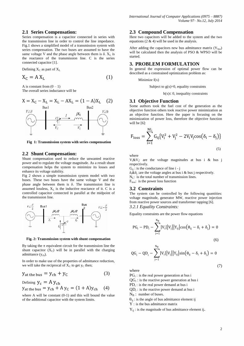
2.1 Series Compensation: Series compensation is a capacitor connected in series with

the transmission line in order to control the line impedance.

Fig.1 shows a simplified model of a transmission system with

series compensation. The two buses are assumed to have the

same voltage V and the phase angle between them is δ. XL is

the reactance of the transmission line. C is the series

connected capacitor [1].

Defining XC as part of XL

(1)

A is constant from (0 – 1)

The overall series inductance will be

(2)

Fig 1: Transmission system with series compensation

2.2 Shunt Compensation: Shunt compensation used to reduce the unwanted reactive

power and to regulate the voltage magnitude. As a result shunt

compensation helps the system to minimize its losses and

enhance its voltage stability.

Fig 2 shows a simple transmission system model with two

buses. These two buses have the same voltage V and the

phase angle between them is . The transmission line is

assumed lossless, XL is the inductive reactance of it. C is a

controlled capacitor connected in parallel at the midpoint of

the transmission line.

Fig. 2: Transmission system with shunt compensation

By taking the equivalent circuit for the transmission line the

shunt capacitor (XC) will be in parallel with the charging

admittance (ych).

In order to make use of the properties of admittance reduction,

we will take the reciprocal of XC to get yC then;

(3)

Defining (4)

where A will be constant (0-1) and this will bound the value

of the additional capacitor with the system limits.

2.3 Compound Compensation Here two capacitors will be added to the system and the two

equations (2 & 4) will be used in the analysis.

After adding the capacitors new bus admittance matrix (Ybus)

will be calculated then the analysis of PSO & WPSO will be

started.

3. PROBLEM FORMULATION In general the expression of optimal power flow can be

described as a constrained optimization problem as:

Minimize f(x)

Subject to g(x)=0, equality constraints

h(x) 0, inequality constraints

3.1 Objective Function Some authors took the fuel cost of the generation as the

objective function others took reactive power minimization as

an objective function. Here the paper is focusing on the

minimization of power loss, therefore the objective function

will be [6]:

(5)

where

Vi&Vj: are the voltage magnitudes at bus i & bus j

respectively.

Gij : is the conductance of line i - j

δi&δj :are the voltage angles at bus i & bus j respectively.

NL: is the total number of transmission lines.

Floss: is the power loss function

3.2 Constraints The system can be controlled by the following quantities:

voltage magnitude, generator MW, reactive power injection

from reactive power sources and transformer tapping [6].

3.2.1 Equality Constraints:

Equality constraints are the power flow equations

(6)

(7)

where

PGi : is the real power generation at bus i

QGi : is the reactive power generation at bus i PDi : is the real power demand at bus i

QDi : is the reactive power demand at bus i

NB : number of buses. ij : is the angle of bus admittance element ij

Y : is the bus admittance matrix Yij : is the magnitude of bus admittance element ij.



3

3.2.2 Inequality Constraints: Limits for each variable [6],

where:

: are the upper and lower limits of voltage

magnitude at bus i

: are the upper and lower limits of tap position of

transformer i

: are the upper and lower limits of reactive

power source i.

: are the upper and lower limits of power

generated by generator i.

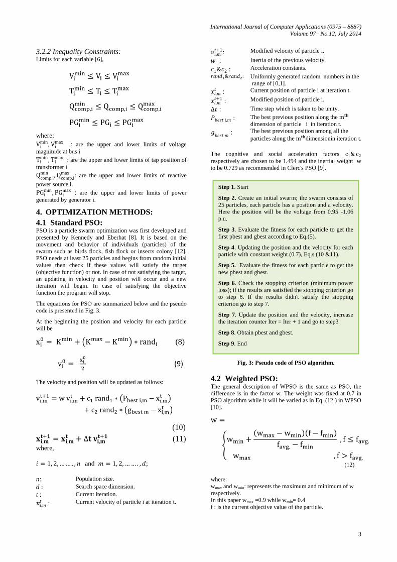
4. OPTIMIZATION METHODS:

4.1 Standard PSO: PSO is a particle swarm optimization was first developed and

presented by Kennedy and Eberhat [8]. It is based on the

movement and behavior of individuals (particles) of the

swarm such as birds flock, fish flock or insects colony [12].

PSO needs at least 25 particles and begins from random initial

values then check if these values will satisfy the target

(objective function) or not. In case of not satisfying the target,

an updating in velocity and position will occur and a new

iteration will begin. In case of satisfying the objective

function the program will stop.

The equations for PSO are summarized below and the pseudo

code is presented in Fig. 3.

At the beginning the position and velocity for each particle

will be

(8)

(9)

The velocity and position will be updated as follows:

(10)

(11)

where,

and ;

n: Population size.

d : Search space dimension.

t : Current iteration.

: Current velocity of particle i at iteration t.

: Modified velocity of particle i.

: Inertia of the previous velocity.

: Acceleration constants.

Uniformly generated random numbers in the

range of [0,1].

: Current position of particle i at iteration t.

: Modified position of particle i.

: Time step which is taken to be unity.

: The best previous position along the

dimension of particle i in iteration t.

: The best previous position among all the

particles along the dimensionin iteration t.

The cognitive and social acceleration factors

respectively are chosen to be 1.494 and the inertial weight

to be 0.729 as recommended in Clerc's PSO [9].

Fig. 3: Pseudo code of PSO algorithm.

4.2 Weighted PSO: The general description of WPSO is the same as PSO, the

difference is in the factor w. The weight was fixed at 0.7 in

PSO algorithm while it will be varied as in Eq. (12 ) in WPSO

[10].

(12)

where:

wmax and wmin: represents the maximum and minimum of w

respectively.

In this paper wmax =0.9 while wmin= 0.4

f : is the current objective value of the particle.

Step 1. Start

Step 2. Create an initial swarm; the swarm consists of

25 particles, each particle has a position and a velocity.

Here the position will be the voltage from 0.95 -1.06

p.u.

Step 3. Evaluate the fitness for each particle to get the

first pbest and gbest according to Eq.(5).

Step 4. Updating the position and the velocity for each

particle with constant weight (0.7), Eq.s (10 &11).


new pbest and gbest.

Step 6. Check the stopping criterion (minimum power

loss); if the results are satisfied the stopping criterion go

to step 8. If the results didn't satisfy the stopping

criterion go to step 7.

Step 7. Update the position and the velocity, increase

the iteration counter Iter = Iter + 1 and go to step3

Step 8. Obtain pbest and gbest.

Step 9. End



4

favg.: is the average objective value of all particles.

fmin.: is the minimum objective value of all particles.

Fig. 4: Pseudo code of WPSO algorithm

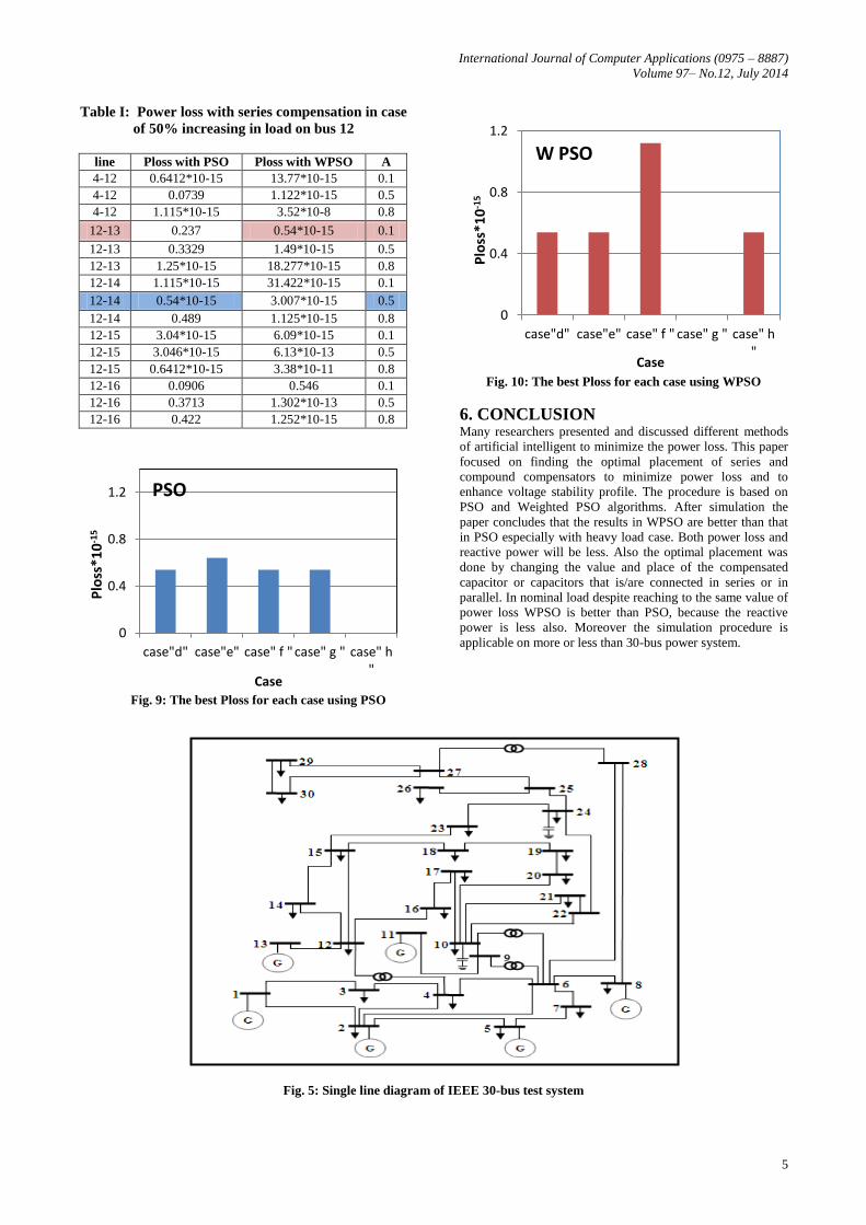
5. RESULTS AND DISCUSSION: The procedure is applied on IEEE 30-bus test system [11].

The single line diagram for this system is shown in Fig. 5. The

system consists from 41 transmission line, 24 load bus, and 6

generator bus (on buses: 1, 2, 5, 8, 11 and 13), bus number 1

is recommended to be the slack bus. PSO and WPSO

algorithms are used in analyzing the system via MATLAB

R2013a environment and run on Intel core i5, 2.4GHz, 4GB.

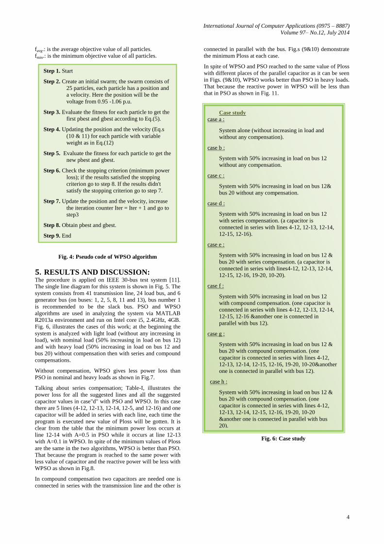
Fig. 6, illustrates the cases of this work; at the beginning the

system is analyzed with light load (without any increasing in

load), with nominal load (50% increasing in load on bus 12)

and with heavy load (50% increasing in load on bus 12 and

bus 20) without compensation then with series and compound

compensations.

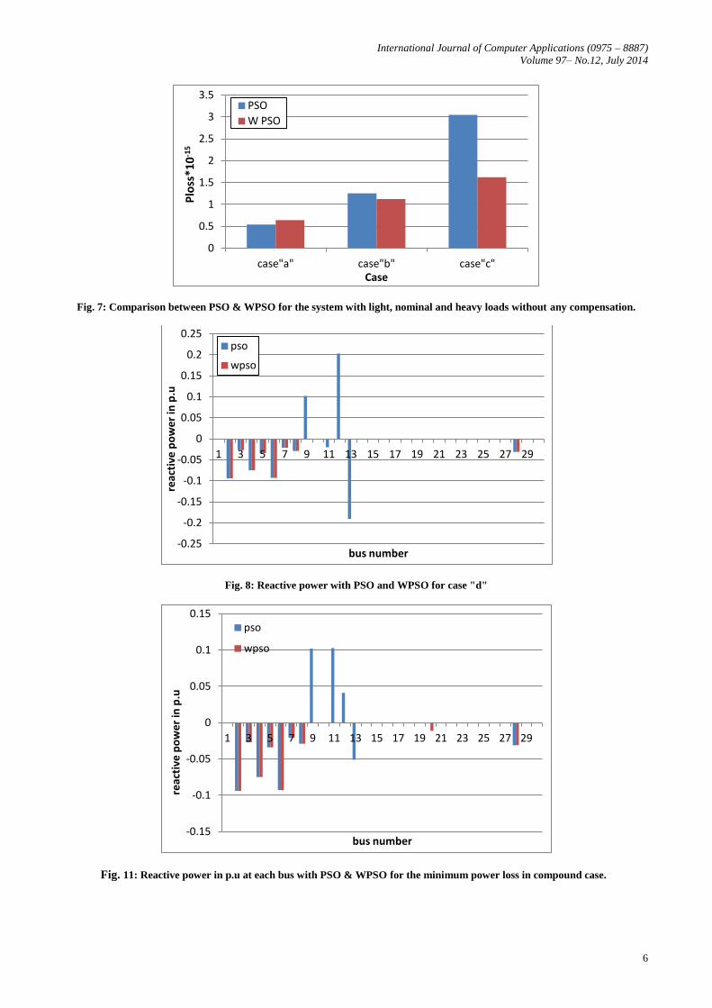
Without compensation, WPSO gives less power loss than

PSO in nominal and heavy loads as shown in Fig.7.

Talking about series compensation; Table-I, illustrates the

power loss for all the suggested lines and all the suggested

capacitor values in case"d" with PSO and WPSO. In this case

there are 5 lines (4-12, 12-13, 12-14, 12-5, and 12-16) and one

capacitor will be added in series with each line, each time the

program is executed new value of Ploss will be gotten. It is

clear from the table that the minimum power loss occurs at

line 12-14 with A=0.5 in PSO while it occurs at line 12-13

with A=0.1 in WPSO. In spite of the minimum values of Ploss

are the same in the two algorithms, WPSO is better than PSO.

That because the program is reached to the same power with

less value of capacitor and the reactive power will be less with

WPSO as shown in Fig.8.

In compound compensation two capacitors are needed one is

connected in series with the transmission line and the other is

connected in parallel with the bus. Fig.s (9&10) demonstrate

the minimum Ploss at each case.

In spite of WPSO and PSO reached to the same value of Ploss

with different places of the parallel capacitor as it can be seen

in Figs. (9&10), WPSO works better than PSO in heavy loads.

That because the reactive power in WPSO will be less than

that in PSO as shown in Fig. 11.

Fig. 6: Case study

Step 1. Start

Step 2. Create an initial swarm; the swarm consists of

25 particles, each particle has a position and

a velocity. Here the position will be the

voltage from 0.95 -1.06 p.u.


first pbest and gbest according to Eq.(5).

Step 4. Updating the position and the velocity (Eq.s

(10 & 11) for each particle with variable

weight as in Eq.(12)


new pbest and gbest.

Step 6. Check the stopping criterion (minimum power

loss); if the results satisfied the stopping

criterion go to step 8. If the results didn't

satisfy the stopping criterion go to step 7.

Step 7. Update the position and the velocity, increase

the iteration counter Iter = Iter + 1 and go to

step3

Step 8. Obtain pbest and gbest.

Step 9. End

Case study

case a :

System alone (without increasing in load and

without any compensation).

case b :

System with 50% increasing in load on bus 12

without any compensation.

case c :

System with 50% increasing in load on bus 12&

bus 20 without any compensation.

case d :


with series compensation. (a capacitor is

connected in series with lines 4-12, 12-13, 12-14,

12-15, 12-16).

case e :

System with 50% increasing in load on bus 12 &

bus 20 with series compensation. (a capacitor is

connected in series with lines4-12, 12-13, 12-14,

12-15, 12-16, 19-20, 10-20).

case f :


with compound compensation. (one capacitor is

connected in series with lines 4-12, 12-13, 12-14,

12-15, 12-16 &another one is connected in

parallel with bus 12).

case g :


bus 20 with compound compensation. (one

capacitor is connected in series with lines 4-12,

12-13, 12-14, 12-15, 12-16, 19-20, 10-20&another

one is connected in parallel with bus 12).

case h :


bus 20 with compound compensation. (one

capacitor is connected in series with lines 4-12,

12-13, 12-14, 12-15, 12-16, 19-20, 10-20

&another one is connected in parallel with bus

20).



5

Table I: Power loss with series compensation in case

of 50% increasing in load on bus 12

line Ploss with PSO Ploss with WPSO A

4-12 0.6412*10-15 13.77*10-15 0.1

4-12 0.0739 1.122*10-15 0.5

4-12 1.115*10-15 3.52*10-8 0.8

12-13 0.237 0.54*10-15 0.1

12-13 0.3329 1.49*10-15 0.5

12-13 1.25*10-15 18.277*10-15 0.8

12-14 1.115*10-15 31.422*10-15 0.1

12-14 0.54*10-15 3.007*10-15 0.5

12-14 0.489 1.125*10-15 0.8

12-15 3.04*10-15 6.09*10-15 0.1

12-15 3.046*10-15 6.13*10-13 0.5

12-15 0.6412*10-15 3.38*10-11 0.8

12-16 0.0906 0.546 0.1

12-16 0.3713 1.302*10-13 0.5

12-16 0.422 1.252*10-15 0.8

Fig. 9: The best Ploss for each case using PSO

Fig. 10: The best Ploss for each case using WPSO

6. CONCLUSION Many researchers presented and discussed different methods

of artificial intelligent to minimize the power loss. This paper

focused on finding the optimal placement of series and

compound compensators to minimize power loss and to

enhance voltage stability profile. The procedure is based on

PSO and Weighted PSO algorithms. After simulation the

paper concludes that the results in WPSO are better than that

in PSO especially with heavy load case. Both power loss and

reactive power will be less. Also the optimal placement was

done by changing the value and place of the compensated

capacitor or capacitors that is/are connected in series or in

parallel. In nominal load despite reaching to the same value of

power loss WPSO is better than PSO, because the reactive

power is less also. Moreover the simulation procedure is

applicable on more or less than 30-bus power system.

Fig. 5: Single line diagram of IEEE 30-bus test system

0

0.4

0.8

1.2

case"d" case"e" case" f " case" g " case" h "

Plo

ss*1

0-1

5

Case

PSO

0

0.4

0.8

1.2

case"d" case"e" case" f " case" g " case" h "

Plo

ss*1

0-1

5

Case

W PSO



6

Fig. 7: Comparison between PSO & WPSO for the system with light, nominal and heavy loads without any compensation.

Fig. 8: Reactive power with PSO and WPSO for case "d"

Fig. 11: Reactive power in p.u at each bus with PSO & WPSO for the minimum power loss in compound case.

0

0.5

1

1.5

2

2.5

3

3.5

case"a" case"b" case"c"

Plo

ss*1

0-1

5

Case

PSO

W PSO

-0.25

-0.2

-0.15

-0.1

-0.05

0

0.05

0.1

0.15

0.2

0.25

1 3 5 7 9 11 13 15 17 19 21 23 25 27 29

reac

tive

po

we

r in

p.u

bus number

pso

wpso

-0.15

-0.1

-0.05

0

0.05

0.1

0.15

1 3 5 7 9 11 13 15 17 19 21 23 25 27 29

reac

tive

po

we

r in

p.u

bus number

pso

wpso



7

7. REFERENCES [1] Hasan Dağ, Banu Öztürk and Aysu Özyürek,

"Application of series and shunt compensation to Turkish

national power transmission system to improve system

load ability", ELECO99 international conference on

electrical and electronics engineering (Eo1.101/A2-

61),1999, pp.243-247.

[2] Ulas Eminoglu, M. Hakan Hocaoglu and Tankut

Yalcinoz, "Transmission line shunt and series

compensation with voltage sensitive loads", International

Journal of Electrical Engineering Education 46/4,2009,

pp:354-369,

[3] Om Prakash Mahela& Sheesh Ram Ola, "Comparison of

HT Shunt Capacitors and SVC for Active and Reactive

Power Flow Control in Transmission Line: the Case of

RRVPNL Power Grid", International Journal of

Electrical and Electronics Engineering (IJEEE), ISSN

2278-9944, Vol. 2, Issue 1, Feb 2013,pp: 49-58

[4] Prasanthi P. S, Hazeena K .A ,"Improved Particle Swarm

Optimization Based Loss Minimization", International

Journal of Advanced Research in Electrical, Electronics

and Instrumentation Engineering, Vol. 2, Special Issue 1,

December 2013, ISSN (Print) : 2320 – 3765, ISSN

(Online): 2278 – 8875, pp: 21-29. India.

[5] Altaf Badar, Dr. B.S. Umre, and Dr. A. S. Junghare,

"Study of Artificial Intelligence Optimization

Techniques applied to Active Power Loss Minimization",

IOSR Journal of Electrical and Electronics Engineering

(IOSR-JEEE) e-ISSN: 2278-1676, p-ISSN: 2320-3331

PP 39-45 www.iosrjournals.org.

International Conference on Advances in Engineering &

Technology – 2014 (ICAET-2014)

[6] Numphetch Sinsuphun, Uthen Leeton, Umaporn

Kwannetr, "Loss Minimization Using Optimal Power

Flow Based on Swarm Intelligences", ECTI Transactions

on Electrical Eng., Electronics, and Communications

Vol.9, NO.1 February 2011, pp:212-222.

[7] Xiao-Ping Zhang, Christian Rehtanz and Biksh Pal,

"Flexible AC transmission systems modeling and control

", springer-verlag Berlin Heidelberg 2006. Printed in

Germany.

[8] Kennedy, J. and R. Eberhart, \Particle swarm

optimization," IEEE Proc. International Conference on

Neural Networks, 1942-1948, Perth, Aust, November

1995.

[9] M. Clerc, “The Swarm and the Queen: Towards a

Deterministic and Adaptive Particle Swarm

Optimization”, Proceedings of Congress on Evolutionary

Computation, Annecy, France, vol. 3, pp. 1951-1957,

06-09 July, 1999.

[10] Chai, J. Li, Y. Zhang, M. Jiang, and Y. Xu, “Intelligent

Optimization Method of PSS Parameters Based on Grid

Equivalence”, International Conference on Electrical and

Control Engineering (ICECE), Yichang, China, 16-18

Sept. 2011.

[11] R. Zimmerman, C. E. Murillo-Sanchez, and D. Gan,

“MATPOWER: A MATLAB power system simulation

package”, Cornell University, Ithaca, NY, 2008.

[Online]. Available:

http://www.pserc.cornell.edu/matpower/

[12] S J Bassi, M K Mishra and E E Omizegba, Automatic

Tuning of Proportional–Integral–Derivative (PID)

Controller using Particle Swarm Optimization (PSO)

Algorithm. International Journal of Artificial Intelligence

& Applications (IJAIA), 2011.vol.2, no.4, pp:25-34.

IJCATM : www.ijcaonline.org

Date post:	11-Mar-2018
Category:	Documents
Upload:	lamdang
View:	221 times
Download:	4 times

Optimal Placement of Series and Compound Compensators...

Documents