Optimal Portfolio Liquidationwith Dynamic Coherent Risk

Andrey Selivanov1 Mikhail Urusov2

1Moscow State University and Gazprom Export

2Ulm University

Analysis, Stochastics, and Applications. A Conference in Honour ofWalter Schachermayer – Vienna University, July 12–16, 2010

Outline

Optimal Portfolio Liquidation

Dynamic Risk

Main Result

Outline

Optimal Portfolio Liquidation

Dynamic Risk

Main Result

A trader sells x > 0 shares of a stock in an illiquid market. Inselling the price falls from S− to

S+ = S− −1q

x .

The trader gets the payout

x(

S− −1

2qx)

︸ ︷︷ ︸average price per share

instead of xS−

OPL How to sell optimally X0 shares until time N?

X0, N are specified by a client, X0 is very big

Time horizon is usually short

A strategy is a sequence x = (xi)Ni=0, where all xi ≥ 0 and∑N

i=0 xi = X0

xi means the number of shares to sell at time i , i = 0, . . . ,N

X (resp., Xdet) denotes the set of adapted (resp., deterministic)strategies

Model for unaffected priceA random walk (Sn) (short time horizon)

Model for price impactA block-shaped limit order book with infinite resilience

Optimization problemMinimize a certain dynamic coherent risk measure

Model for price impact

Linear permanent and temporary impacts with the coefficientsγ ≥ 0 resp. κ > 0

Selling xk ≥ 0 shares at times k , k = 0,1, . . . :

Sn+ = Sn− − (κ+ γ)xn,

where Sn− = Sn − γ∑n−1

i=0 xi

Payout at time n:

xn

(Sn− −

κ+ γ

2xn

)Cf. with Bertsimas and Lo (1998), Almgren and Chriss (2001)

LOB with finite resilience:Obizhaeva and Wang (2005), Alfonsi, Fruth, and Schied (2010)

Notation Xn := X0 −∑n−1

i=0 xi , n = 1, . . . ,N + 1, the number ofshares remaining at hand at time n−. Note that XN+1 = 0

(xi)←→ (Xi)

Properties of strategies desirable for practitioners

(A) Dynamic consistency

(B) Presence of an intrinsic time horizon N∗ such that

N∗ < N for small X0,N∗ = N for large X0,N∗ is increasing as a function of X0

(C) Relative selling speed decreasing in the position size:

x0X0

decreases as a function of X0

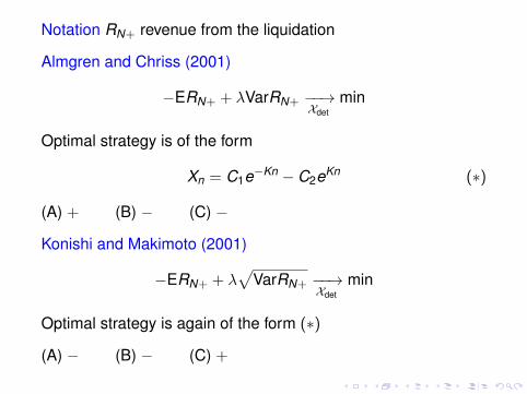
Notation RN+ revenue from the liquidation

Almgren and Chriss (2001)

−ERN+ + λVarRN+ −−→Xdetmin

Optimal strategy is of the form

Xn = C1e−Kn − C2eKn (∗)

(A) + (B) − (C) −

Konishi and Makimoto (2001)

−ERN+ + λ√

VarRN+ −−→Xdetmin

Optimal strategy is again of the form (∗)

(A) − (B) − (C) +

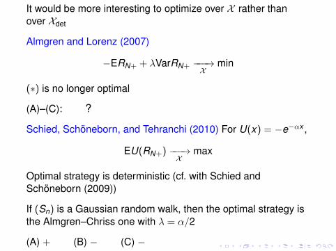
It would be more interesting to optimize over X rather thanover Xdet

Almgren and Lorenz (2007)

−ERN+ + λVarRN+ −−−→X min

(∗) is no longer optimal

(A)–(C): ?

Schied, Schoneborn, and Tehranchi (2010) For U(x) = −e−αx ,

EU(RN+) −−−→X

max

Optimal strategy is deterministic (cf. with Schied andSchoneborn (2009))

If (Sn) is a Gaussian random walk, then the optimal strategy isthe Almgren–Chriss one with λ = α/2

(A) + (B) − (C) −

Outline

Optimal Portfolio Liquidation

Dynamic Risk

Main Result

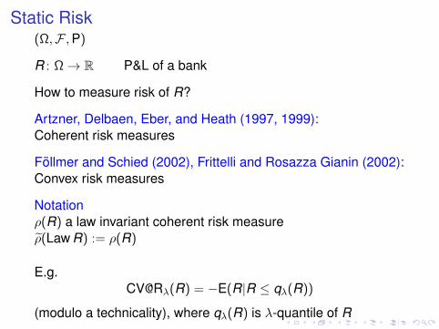
Static Risk(Ω,F ,P)

R : Ω→ R P&L of a bank

How to measure risk of R?

Artzner, Delbaen, Eber, and Heath (1997, 1999):Coherent risk measures

Follmer and Schied (2002), Frittelli and Rosazza Gianin (2002):Convex risk measures

Notationρ(R) a law invariant coherent risk measureρ(Law R) := ρ(R)

E.g.CV@Rλ(R) = −E(R|R ≤ qλ(R))

(modulo a technicality), where qλ(R) is λ-quantile of R

Dynamizing ρ

(Ω,F , (Fn)Nn=0,P)

Cashflow F = (Fn)Nn=0: an adapted process

Fn means P&L of a bank at time n

Need to define dynamic risk ρ(F )

ρ(F ) = (ρn(F ))Nn=0 an adapted process

ρn(F ) ≡ ρ(Fn, . . . ,FN) means the risk of the remaining part(Fn, . . . ,FN) of the cashflow measured at time n

Define inductively:ρN(F ) = −FN ,

ρn(F ) = −Fn + ρ(

Law[−ρn+1(F )|Fn]), n = N − 1, . . . ,0

Cf. with Riedel (2004), Cheridito and Kupper (2006), Cherny(2009)

Outline

Optimal Portfolio Liquidation

Dynamic Risk

Main Result

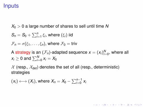
Inputs

X0 > 0 a large number of shares to sell until time N

Sn = S0 +∑n

i=1 ξi , where (ξi) iid

Fn = σ(ξ1, . . . , ξn), where F0 = triv

A strategy is an (Fn)-adapted sequence x = (xi)Ni=0, where all

xi ≥ 0 and∑N

i=0 xi = X0

X (resp., Xdet) denotes the set of all (resp., deterministic)strategies

(xi)←→ (Xi), where Xn = X0 −∑n−1

i=0 xi

Problem Settings

Setting 1 For a strategy x = (xi)Ni=0 define the cashflow F x by

F xn = xn

(Sn − γ

∑n−1i=0 xi − κ+γ

2 xn

), n = 0, . . . ,N.

The problem: ρ0(F x ) −→ min over x ∈ X

Setting 2 For a strategy x define Gx by Gx0 = 0 and

Gxn = xn−1

(Sn−1 + ξn

2 − γ∑n−2

i=0 xi − κ+γ2 xn−1

),

n = 1, . . . ,N + 1.

The problem: ρ0(Gx ) −→ min over x ∈ X

Main Result

Standing assumption 0 < ρ(Law ξ) <∞

Set a := ρ(Law ξ)/κ, so a > 0

Theorem Optimal strategy is the same in both settings.Moreover, it is deterministic and given by the formulas

xi =X0

N∗ + 1+ a

(N∗

2− i), i = 0, . . . ,N∗,

xi = 0, i = N∗ + 1, . . . ,N,

where

N∗ = N ∧

(ceil−1 +

√1 + 8X0/a2

− 1

)with ceil y denoting the minimal integer d such that y ≤ d

Discussion

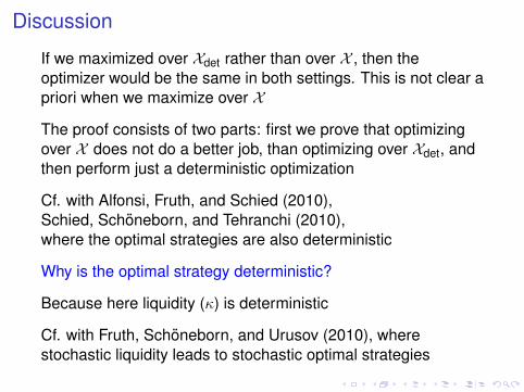
If we maximized over Xdet rather than over X , then theoptimizer would be the same in both settings. This is not clear apriori when we maximize over X

The proof consists of two parts: first we prove that optimizingover X does not do a better job, than optimizing over Xdet, andthen perform just a deterministic optimization

Cf. with Alfonsi, Fruth, and Schied (2010),Schied, Schoneborn, and Tehranchi (2010),where the optimal strategies are also deterministic

Why is the optimal strategy deterministic?

Because here liquidity (κ) is deterministic

Cf. with Fruth, Schoneborn, and Urusov (2010), wherestochastic liquidity leads to stochastic optimal strategies

Remarks

I (A) + (B) + (C) +

(recall “+−−” for the Almgren–Chriss strategy)

I (Xn) parabola vs. Xn = C1e−Kn − C2eKn

(Almgren–Chriss is now a benchmark for practitioners)

I Setting N =∞ (time horizon is not specified by the client)we get a strategy with a purely intrinsic time horizon N∗.Cf. with Almgren (2003), Schoneborn (2008)

I a ↑ leads to a quicker liquidation in the beginning

=⇒ reasonable dependence of the liquidation strategy onvolatility risk (ρ(Law ξ)) and on liquidity risk (κ)

Thank you for your attention!

Possible Generalizations

I More general price impact?

Optimal strategies are again deterministic

I Convex risk measure ρ?

Optimal strategies are again deterministic, however,different in Settings 1 and 2

Typically (A) + (B) −

Also (C) − in an example with entropic riskmeasure, which was worked out explicitly

Alfonsi, A., A. Fruth, and A. Schied (2010).Optimal execution strategies in limit order books with general

shape functions.Quantitative Finance 10(2), 143–157.

Almgren, R. (2003).Optimal execution with nonlinear impact functions and

trading-enhanced risk.Applied Mathematical Finance 10, 1–18.

Almgren, R. and N. Chriss (2001).Optimal execution of portfolio transactions.Journal of Risk 3, 5–39.

Almgren, R. and J. Lorenz (2007).Adaptive arrival price.In Algorithmic Trading III: Precision, Control, Execution. Ed.:

Brian R. Bruce, Institutional Investor Journals.

Artzner, P., F. Delbaen, J.-M. Eber, and D. Heath (1997).Thinking coherently.

Risk 10(11), 68–71.

Artzner, P., F. Delbaen, J.-M. Eber, and D. Heath (1999).Coherent measures of risk.Math. Finance 9(3), 203–228.

Bertsimas, D. and A. Lo (1998).Optimal control of execution costs.Journal of Financial Markets 1, 1–50.

Follmer, H. and A. Schied (2002).Convex measures of risk and trading constraints.Finance Stoch. 6(4), 429–447.

Frittelli, M. and E. Rosazza Gianin (2002).Putting order in risk measures.Journal of Banking an Finance 26(7), 1473–1486.

Konishi, H. and N. Makimoto (2001).Optimal slice of a block trade.Journal of Risk 3(4).

Obizhaeva, A. and J. Wang (2005).Optimal trading strategy and supply/demand dynamics.Available at SSRN: http://ssrn.com/abstract=686168.

Schied, A. and T. Schoneborn (2009).Risk aversion and the dynamics of optimal liquidation

strategies in illiquid markets.Finance Stoch. 13(2), 181–204.

Schied, A., T. Schoneborn, and M. Tehranchi (2010).Optimal basket liquidation for CARA investors is

deterministic.To appear in Applied Mathematical Finance.