Optimal Power Flow Competition Introduction Tim Heidel Program Director Advanced Research Projects Agency – Energy (ARPA-E) U.S. Department of Energy GRID DATA Kickoff Meeting Denver, CO, March 30-31, 2016
Transcript
Optimal Power Flow
Competition Introduction
Tim HeidelProgram Director
Advanced Research Projects Agency – Energy (ARPA-E)
U.S. Department of Energy
GRID DATA Kickoff Meeting
Denver, CO, March 30-31, 2016
Electric grid operations
OPF
OPF
OPF
OPF
OPFOPF
OPF
depend on OPF
1
Optimizing Grid Power Flows is Hard
392 IEEE TRANSACTIONS ON POWER SYSTEMS, VOL. 16, NO. 3, AUGUST 2001
Fig. 3. Two bus system.
Fig. 4. Power circles and solution boundary curve. Contours of .
V. EXAMPLES
A. Two Bus System
The numerical results obtained using the continuation algo-
rithm described earlier may be verified analytically for a two
bus system, such as shown in Fig. 3. In this system, Gen1 is a
slack bus, Bus2 is a PQ bus, and pu.
Eliminating from the real and reactive power balance equa-
tions for Bus2 results in equations for power circles in the –
plane,
These curves (circles) are shown in Fig. 4 as dashed lines. Each
circle corresponds to a different value of . There exists a
boundary in the – plane beyond which there are no power
flow solutions. At any point on that boundary, the power flow
Jacobian is singular. It can easily be shown that points which
lie on the boundary, i.e., that satisfy the power flow equations
along with the requirement , are given by,
Hence the solution boundary curve in the – plane is a
parabola (remembering that and are fixed).
The solution boundary can be computed numerically by
making the following observation. In – space, with held
constant, boundary points occur when there is a change in the
number of solutions as is varied. The dashed curves of Fig. 5
show solutions for various (fixed) values of . (These curves
are analogous to Fig. 1. In this example is and is .)
Using the continuation technique, and allowing to be a free
parameter, the boundary curve in – space can be computed.
It is shown in Fig. 5 as a solid curve. The same curve plotted
Fig. 5. curves and solution boundary curve. Contours of .
Fig. 6. Three bus system.
in – space is shown as a solid curve in Fig. 4. Note that
it has the predicted parabolic form. Furthermore, it forms the
boundary of the power circle diagrams and is tangential to the
circles.
It is interesting to note that the contours (dashed lines) of
Fig. 4 correspond to horizontal slices through Fig. 5, and the
contours of Fig. 5 correspond to horizontal slices through Fig. 4.
Together they provide a picture of the solution space in – –
space.
B. Three Bus System
This example explores the solution space boundary for the
system of Fig. 6. Even though the system is small, it illustrates
the complexity of the power flow solution space. The solution
space boundary will be investigated for two cases. The first con-
siders the boundary when and are free to vary, whilst the
second presents nomograms of versus . The connection
between these two cases will also be explored.
1) Case 1: versus : The power flow solution space
projected onto the – plane is shown in Fig. 7. In this figure,
each curve corresponds to a distinct value of . The outer
boundary of the solution space is clear. However there is also
some folding within the solution space. The continuation tech-
nique can be used to locate all the boundary curves, including
the inner folds.
Finding the boundary points amounts to finding those points
where, if is held constant and is varied (or vice-versa),
there is a change in the number of power flow solutions. Fig. 8
shows the power-angle curves at Gen1 for various values of .
TABLE IBASE CASE PROPERTIES AND ECONOMIC DISPATCH RESULTS FOR THREE SCENARIOS: (A) NORMAL OPERATION WITH AND WITHOUT VOLTAGE
OPTIMIZATION (CASES 1&2); (B) NORMAL OPERATION (RETIRED PLANTS) WITH AND WITHOUT VOLTAGE OPTIMIZATION ((CASES 3&4); (C)ECONOMIC DISPATCH WITH 6% RESERVE WITH AND WITHOUT VOLTAGE OPTIMIZATION (CASES 5&6)
in Scenarios A and B but simulates the 6% required
real power generation reserve by assuming that each
load has increased by 6%. This closely emulates the
detailed requirement that each LSE provides this amount
of reserve in proportion to its own load. Shown in Table I
is the summary of results with such uniformly distributed
reserves over all 52 LSEs within PJM. One can see that
the overall generation cost required to meet uniformly
increased load is increased relative to the total generation
cost when not requiring such reserve. Total load charges
are significantly increased in the Case 5 when generator
voltages are not optimized; however, load charges are
reduced significantly in Case 6 when generator voltages
are optimized; an LSE could see close to 10% of load
charge savings when required to support reserve if gener-
ator voltage is optimized. Notice that merchandise surplus
is positive and significantly smaller in Case 6 than in Case
5 when voltage is fixed.
It follows from the results in Table I that voltage op-
timization would result in major savings. It follows from
comparing Cases 1 and 2 in Scenario A that operating during
normal conditions with and without optimization would lead
to around 9% savings, and, assuming each day the same, to
$1.3 billion per year. Similarly, compare Cases 2 and 5. Case
2 corresponds to true corrective resource management that
responds as contingencies happen; it does not require unused
reserve. In contrast, Case 5 corresponds to today’s market
practice which does require unused reserve. Case 2 offers a
15% savings over Case 5. This would amount to a $2.3 billion
savings per year. Finally, by comparing cost when operating
with today’s reserve and optimized voltage (Case 6) to the
cost of operating fixed voltage with no reserve (Case 1) one
concludes that the two are almost the same. This means that
one can still have reserve, but reduce total generation cost
significantly when compared to today’s cost. The numbers are
truly revealing.
V. RECOMMENDED NEXT STEPS
In closing, while the effects of optimized resource allo-
cation, generators in particular, are system- and scenario-
dependent, the above example PJM analysis indicates several
general benefits. Optimizing real power generation over power
flow always leads to a decreased total generation cost needed
to supply given load. This means that optimizing generation
cost (economic efficiency) is more important than minimizing
delivery loss (physical efficiency) when performing economic
dispatch. Also, when comparing all scenarios with and without
generator voltage optimization, one concludes that voltage op-
timization invariably reduces total generation cost significantly
and, by doing this, reduces load charges. It is shown that
depending on operating practices in place, the cost savings
may be between 9% and 15%. Voltage optimization further
makes LMPs always positive and less volatile. All these
features are critical for operating and planning future elec-
tricity markets more efficiently. While a paradigm for reliable
resource management envisioned here seems like a very distant
future, it is fundamentally straightforward to implement and
the payoffs would be huge. Finally, it was shown that all else
being the same, flexible resource management accommodates
higher deployment of renewable generation by supporting
long-distance delivery; as a result, it is key to pollution
reduction [11]. This cannot be done without good software and
reliable communications for remote equipment management.
If done right, it could become a true game changer.
REFERENCES
[1] PJM Manual for Operations Planning, PJM 2014.[2] 2013 Annual Report on Market Issues & Performance, California ISO.[3] Voltage Dispatch and Pricing in Support of Efficient Real Power Dispatch,
NETSS NYSERDA Report 10476, 2012.[4] Private discussions with Robin Podmore, Incremental Systems, Inc.,
November 2014.[5] Market-based regulation, November 2014, PJM site.[6] PJM Transmission Operating Manual, PJM site.[7] Ilic, M., Lang, J., Litvinov, E., Luo, X., Tong, J., Fardanesh, B.,
Stefopoulos, “Toward the Coordinated Voltage Control (CVC)-EnabledSmart Grids”, IEEE PES Innovative Smart Grid Technologies (ISGT),Dec. 5-7, 2011, Manchester, UK.
[8] Guo, Q, Sun, H., Zhang, M., Tong, J., Zhang, B., “Optimal VoltageControl of PJM smart Transmission Grid: Study, Implementation andEvaluation”, IEEE Trans. on Smart Grid, September 2013.
[9] Stott, B.; Alsac, O., ”Basic Requirements for Real-Life Problems andTheir Solutions”, White paper, July 2012.
[10] Ilic, M. (PI), Standards for Dynamics, PSERC S-55 project, 2014.[11] Ilic, M., Engineering IT-Enable Sustainable Electricity Services”,
Springer 2013.
No Voltage Dispatch (DC-OPF)
Voltage Dispatch (AC-OPF)
Savings: $117,637 (6.8%)
M. Ilic et al., “Optimal voltage management for enhancing
electricity market efficiency” FERC Staff Technical Conference, June 20144
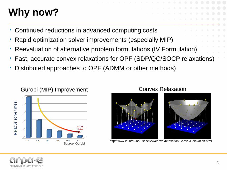
Why now?
‣ Continued reductions in advanced computing costs