Page 1
203
AMSE JOURNALS-AMSE IIETA publication-2017-Series: Advances A; Vol. 54; N°2; pp 203-220
Submitted Mar. 09, 2017; Revised Apr. 17, 2017; Accepted May 02, 2017
Optimal Pricing and Admission Control of Markovian Queueing
System with Negative Customers
*Zaiming Liu, **Wei Deng, ***Gang Chen
* School of Mathematics and Statistics, Central South University, Changsha 410083, China
([email protected] )
** School of Mathematics and Statistics, Central South University, Changsha 410083, China
([email protected] )
*** School of Mathematics and Statistics, Central South University, Changsha 410083, China
([email protected] )
Abstract
This paper analyses the optimal dynamic pricing and admission control policies to maximize
the average benefit in a Markovian queue with negative customers. The negative customers, as a
type of job cancellation signals, are frequently employed to solve the congestion problem in the
production system. In our model, the manager proposes a price for positive customers, and decide
whether or not to accept the arriving negative customers in any decision epoch. Treating the
problem as a Markov decision process, the author derived the monotonicity of the optimal pricing
policy, proved the optimal admission policy as a threshold policy, and verified the monotonicity of
the threshold policy in system parameters. Finally, some numerical experiments were presented to
depict the effect of system parameters on the optimal policy and average benefit.
Key words
Queueing system, Dynamic pricing, Admission control, Markov decision process, Negative
customers.
1. Introduction
Page 2
204
Recently, there has been a growing interest in Markovian queueing systems with negative
customers. Unlike ordinary customers, the negative customers require no service and reduce a
queue of ordinary customers a nonempty queueing system [1]. Over the years, queueing models
with negative customers into have been extensively applied in performance optimization of
production inventory systems, service organizations and computer systems. The implementation
has aroused wide-ranging theoretical interests and given birth to diverse practical applications. In
signal systems, negative customers are represented as inhibition signals, i.e., the instructions to
cancel requests for resources [2,3]. In database systems, negative customers act as instructions to
halt the operations made impossible by data locking [4-6]. In neural networks, negative and positive
customers serve as inhibitory and excitatory signals, respectively. In inventory systems, negative
customers stand for signals to dispose items in the serviceable inventory [7,8].
To improve the management of queueing systems in different industries, much research has
been done on the dynamic pricing and admission control problems. However, rarely has any scholar
explored the dynamic control of the queues with negative customers. Considering the popularity
of such queues, it is meaningful to study the optimal control of the queues with negative customers.
The purpose of dynamic pricing is to enhance network manager’s ability to recover costs and make
benefits, thus promoting capacity expansions. In optimal pricing problems, the customers are
assumed to accept a highest consumption price, which is a random variable called the reservation
price, and the manager is assumed to state a price at any decision epoch [9,10].
Low [11] pioneered the study of dynamic optimal pricing problems. He derived the
monotonicity of the optimal prices in the queue length. Son [10] examined the optimal pricing
control problem from the perspectives of deterministic service times and side-line benefit. Yoon
and Lewis [12] disclosed the monotonicity of a queueing system with periodically varying
parameters. Similar monotonicity results were also derived for the make-to-stock queue model in
a production inventory system [13]. Cil et al. [14] explored an optimal dynamic pricing problem
for a two-class queueing system, concluding that the optimal pricing control depends on the queue
length vector. Feinberg et al. [15] studied the optimal pricing of a GI/M/k/N queue involving
different types of customers and holding costs.
Being a provisioning strategy to limit the number of customers in a system, admission control
is essential to packet-switched networks, as it is capable of relieving the traffic congestion. Heyman
[16] was the first to study the optimal admission control problems. The early papers on admission
control of queueing systems were summarized by Stidham [17]. Yoon and Lewis [12] opened the
new research field of admission control in periodic nonstationary queueing systems. Son [10]
discussed the optimal admission control of a service company with two classes of customers. Wu
Page 3
205
et al. [18] investigated the multiple product admission control in semiconductor production systems
under the constraint of process queue time (PQT).
The structural properties of optimal pricing and admission control were widely discussed by
Koole [19] and Lin et al. [20]. As far as we know, however, no report has been released on the
pricing policy and admission control of queues with negative customers prior to our research. To
make up for the gap, this paper probes into the structure of optimal pricing and admission control
policies in a queueing system with negative customers. The goal is to find the optimal policy that
yields the maximum average benefit over an infinite horizon. To this end, the system manager must
weigh the penalty and holding cost against reward. Furthermore, this research is motivated by the
vision that the wide applications of negative customers may offer a mechanism to curb the
excessive congestion of production inventory systems. Specifically, the pricing control of positive
customers were considered as the balk behaviour of customer demand, the negative customers were
regarded as the disposal of items or the transition to the secondary market, and the manager decided
whether or not to accept the negative customers, seeking to reduce the excess items in the inventory.
The research findings help to improve the management of inventory systems, and enable the
manager to achieve the maximum average benefit via the optimal control policy.
The main contributions of this research are as follows. First, to the best of our knowledge, this
research is the first to investigate the optimal pricing and admission control policies in a queueing
system with negative customers, which fills a gap in the research into the control of queues with
negative customers. Second, the author derived the structure of optimal policy and the monotonicity
properties of the optimal pricing and admission threshold. Third, the results obtained in this
research were verified by the numerical results acquired by the Howard’s iteration procedure [21].
The remainder of this paper is organized as follows. Section 2 formulates the model based on
the controllable Markov decision process and derives the optimality equation; Section 3 discusses
the structural properties of the optimal policy in the model; Section 4 examines the effect of system
parameters on the optimal policy and average cost based on several numerical examples; Section
5 wraps up the research with further discussions and conclusions.
2. Model Description
This research focuses on a single-server first-come, first-served (FCFS) queueing system with
negative customers. In the system, the arrivals of positive customers and negative customers are
two independent Poisson processes with the rate of λ+ and λ-, respectively. the service time of each
positive customer is exponentially distributed with rate parameter μ
Page 4
206
For every fixed proposed price r (r[r min, r max]), whenever a positive customer arrives, he/she
either enters the system if his/her reservation price Q exceeds the proposed price or leaves the
system without receiving any reward. It is assumed that Q is a random variable for which the
distribution function and density function are denoted by W(.) and w(.), respectively, and that W——
(r)=1-W(r). The system incurs a holding cost h per positive customer per unit of time. Whenever a
negative customer arrives, he/she is either accepted or rejected by the manager. If the negative
customer is accepted, a positive customer will be killed immediately, and the system will incur a
penalty cost c for the killed customer.
The set of decision epochs consists of the set of all arrivals, service completions, and dummy
transitions due to normalization. In any decision epoch, the manager has to choose a proposed price
r from the set A= [r min, r max] and decide whether or not to accept the negative customer. If the
number of customers in the system at time t is denoted as X(t), then the system evolves as a
continuous-time Markov chain {X(t), t≥0} under any fixed control policy π. It is clear that the
system state space is E= {0, 1, 2, …}. Due to the Markovian property, the optimal policy depends
only on the current state.
The manager is responsible for finding the optimal policy to maximize the long-term average
benefit based on the number of customers in the system. Treating the problem as a Markov decision
process, the author built a discrete-time equivalent of the original queueing system through
normalization. Without loss of generality, it is assumed that that λ++λ-+μ=1. Thus, the total expected
benefit can be obtained as:
where π is the policy; x is the initial state; n is the number of horizons; Eπx is the expectation on
the probability measure determined by the policy and the initial state; M(t) and N(t) are the number
of positive customer and negative customers who have entered the system at time t, respectively;
r(t) is the proposed price at time t. The expectation must exist because the rewards are bounded and
non-negative.
Under the assumption that λ+W——
(rmax)≤μ, the resulting system is a stable queueing system of
finite average queue length and finite average benefit. Assuming that the process {X(t), t≥0} with
state space E is an irreducible, positive recurrent Markov process at each fixed stationary policy π,
Page 5
207
the long-term average benefit of the ergodic Markov process under the policy π can be written as
below in light of Tijms [22].
where pi(π) is a stationary probability of the system under policy π; r (x, a) is the expected benefit
of the system in state x and action a. Let ∏ be the set of all admission policies. The goal is to find
the optimal policy π* that maximizes the long-term average benefit:
To find such a policy, a real-valued function v(x) is defined in the state space. The relative
value function is regarded as the asymptotic difference in total costs if the process starts in state x
instead of some reference states. According to Puterman [21], the optimal policy π* and the optimal
average benefit g are the solutions of the optimality equation below:
(1)
where T is the dynamic programming operator acting on v. The relevant operators are defined as:
The first operator TP v(x) simulates the admission control of the arriving positive customers
based on optimal pricing; the second operator TA v(x) simulates the admission control of arriving
negative customers based on value variation.
The first step to examine the properties of the optimal policy is to investigate the properties of
the relative value function. The key lies in the analysis of the operators TP and TA. The properties
of the relative value function v(x) are defined as follows:
Decreasing: ,
Concavity: ,
Convexity: .
Page 6
208
Referring to Cil et al. [9], it is assumed that a function v(x) has a certain property ϕ preserved
by operator T if the property also belongs to Tv(x). Through the deduction on n in v(x), it is possible
to acquire the properties of the operators TP and TA in our model that preserve the desired properties
(decreasing, concavity, convexity) for the function v(x).
3. Structure of the Optimal Control Policy
This section attempts to derive the optimal policy. The properties of the optimal policy helps
to reduce the solution search space, and ease the computing load in the search of the optimal policy.
The optimality equation (2.1) should be solved before exploring the optimal policy. Whereas
it is hard to solve the equation analytically, the vn+1=Tvn is recursively defined for a random v0
based on the system state transition rate, the stochastic dynamic programming, and the induction
method. It is known that the actions converge to the optimal policy as n→∞. The existence and
convergence of the solutions and optimal policy have been detailed by Aviv and Federgruen [23]
and Sennott [24]. The backward recursion equation is expressed as:
(2)
The main properties of the operators in the system can be summarized by the following lemma
(the proof is given in the Appendix).
Lemma 3.1 For the relative value function v(x) in the model, we have:
(1) The operator TP preserves the properties: Decreasing, Concavity, Convexity,
(2) The operator TA preserves the properties: Decreasing, Concavity, Convexity.
According to the backward recursion equation (3.1), the following properties of the relative
value function v(x) can be obtained based on the above properties of the operators and the induction
method:
, .
On the basis of the structure properties of the relative value function v(x), the structure of the
optimal pricing policy is expressed in the following theorem. Please refer to Cil, E.B [9] for the
proof of the theorem.
Theorem 3.1. The optimal pricing control policy has the following properties:
(1) If W——
(r)/(r W(r)) is strictly decreasing in r[r min, r max], then the optimal pricing is unique;
Page 7
209
(2) If the optimal pricing is non-decreasing in xE, then r*(x)≤r*(x+1) for xE.
Next, the structure of the optimal admission policy was discussed and some conditions were
given to ensure the simplicity of the policy in the model. As mentioned above, the properties of the
optimal policy helps to reduce the solution search space, and ease the computing load in the search
of the optimal policy. Specifically, the structure of the optimal policy was converted as the
properties of the optimal value function and the optimality equation. Following the optimality
equation, the operator T A can be rewritten as:
where H(x-1) =v(x-1)-v(x)-c.
From the above equations, it can be seen that the properties of H(x) should be examined before
deriving the structure of the optimal admission policy. For this purpose, the author presented the
following lemma (the proof is given in the Appendix).
Lemma 3.2. For the admission control problem in the present model, we have:
(1) The function H(x) is increasing for all xE.
(2) If the condition h/μ ≥c holds, then H(0) ≥0.
The admission control problem was analysed in two aspects. First, the acceptance of an arriving
negative customer will incur a penalty cost and the removal of a positive customer. Second, the
rejection of an arriving negative customer will incur a holding cost to the positive customer. Hence,
the system manager must weigh the penalty and holding cost against reward. This means the
decision depends on the number of customers in the system and the parameters h and c .
Theorem 3.2. The optimal admission policy is a threshold policy, that is, the negative
customer should be rejected if x<N*and be accepted if otherwise; N*= min {x: H(x)≥0}; N*=0 if
the condition h/μ ≥c holds.
Proof Since the function H(x) is increasing for all xE (Lemma 3.2 (1)), there must exist an
optimal threshold policy for the admission control problem. Concretely, there exists an N* such
that H(x)≤0 for all states x ≤ N*and H(x)≥0 for all states. Moreover, it states that the negative
customer should be rejected if x ≤ N*and be accepted if otherwise; By the definition of the
admission operator TA, the threshold parameter is N*=min {x: H(x)≥0}; N*=0 if the condition h/μ
≥c holds. From Lemma 3.2 (2), it is obtained that H(x)≥0 for all states xE. Hence, the optimal
admission policy is a pure reception policy, i.e., the negative customer should be accepted for all x
E.
Page 8
210
Intuitively, it is learned that the minimum holding cost is h/μ for a positive customer. If the
condition h/μ ≥c holds, the minimum holding cost for a positive customer must surpass the penalty
cost. To remove the positive customer from the system, the manager has to accept the negative
customer. However, if the condition H(0) ≤0 holds, the manager should decide whether or not to
accept the negative customer based on the number of positive customers in the system. Therefore,
there exists a threshold N*>0 such that the negative customers should be rejected for the states x
≥N*.
Next, the monotonicity properties of the two thresholds m and n were discussed with respect
to various system parameters. Referring to the method in Benjaafar et al. [25] and C¸il et al. [14],
the author compared the optimal value functions of two systems which are identical except for the
value of one parameter, denoted as q. The optimal admission thresholds and optimal value function
corresponding to q are represented by Nq and vq(x), respectively, where q{λ+ , λ-, c, h}.
In order to derive the monotonicity properties of the two thresholds, the properties of the
optimal value function vq(x) in the two systems were examined in light of Koole [19]. To make the
two systems comparable, the normalization rate, depending on {λ+, λ-, μ}, must be constant. The
time was rescaled by a normalization rate τ sufficiently greater than the λ + μ + ξ so that q and q +
ε share the same normalization rate. To maintain a constant normalization rate, the fictitious event
in the two system is τ-q and τ-q-ε, respectively. For instance, if q=μ, the optimality recursion
equations of the system with parameter μ and the system with μ + ε are respectively expressed as:
(3)
(4)
where TP and TA are defined in the previous section. By this method, the following lemma is arrived
at (the proof is given in the Appendix).
Lemma 3.3. For the optimal value function vq(x) of the two systems with different parameters
q, we have:
(1) , ,
(2) , ,
wh er e ∆ v q (x )= v q (x -1 ) - v q (x ) a n d ε≥0 .
Page 9
211
Based on the above properties of optimal value function, the structure of the optimal policy
was obtained by analysing the effect of various system parameters on the thresholds. The results
are summarized in the following theorem.
Theorem 3.3. In the system control problems, the optimal admission threshold N* is non-
decreasing in λ-, c and λ+,h.
Proof In Theorem 3.2, the admission threshold is defined as N*=min {x: H(x)≥0}. According
to the comparison above and Lemma 3.3 (1), it is known that ∆vλ+
+ε(x)≥∆vλ+(x) and ∆vh+ε
(x)≥∆vh(x). Hence, the admission threshold N* is non-increasing in λ+, h. According to Lemma
3.3 (2), ∆vλ-+ε(x)≥∆vλ
-(x) and ∆vc+ε(x)≥∆vc(x), indicating that the admission threshold N* is non-
decreasing in λ -, c.
4. Numerical Examples
Several numerical examples were developed similar to those in [9]. It is assumed that μ=1 and
the proposed price is uniformly distributed in the interval [2, 14]. Whereas Howard’s policy
iteration algorithm is an effective numerical calculation tool for the Markov decision problem, the
algorithm was modified [21] to handle the numerical examples. The examples were designed to
reflect the effect of system state transition on the optimal pricing r*(x), verify the structure of the
optimal admission threshold and average benefit obtained in Section 3, and demonstrate the
response of the optimal policy and average benefit to the system parameters. The observations are
presented in the table and figures below.
Tab.1. Optimal Pricing vs. x for λ+=0.8, λ−=0.3, h=1, c=3
X r∗(x) x r∗(x) x r∗(x) x r∗(x) x r∗(x)
0 1.00 6 1.28 12 2.93 18 5.25 24 6.00
1 1.00 7 1.50 13 3.28 19 5.60 25 6.00
2 1.12 8 1.72 14 3.65 20 5.85 26 6.00
3 1.18 9 2.05 15 4.02 21 6.00 27 6.00
4 1.20 10 2.35 16 4.32 22 6.00 28 6.00
5 1.24 11 2.62 17 4.85 23 6.00 29 6.00
Page 10
212
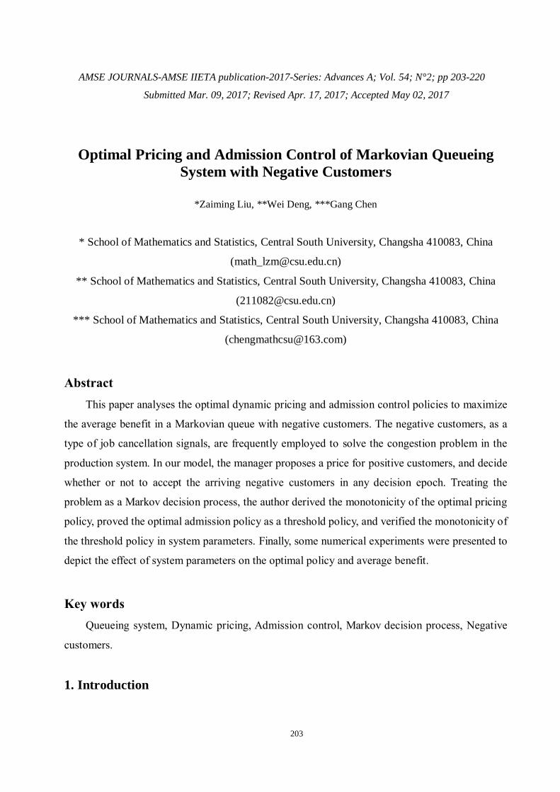
Fig.1. Optimal Threshold and Average Benefit vs. λ+ for λ-=0.3, h-=1, c=3
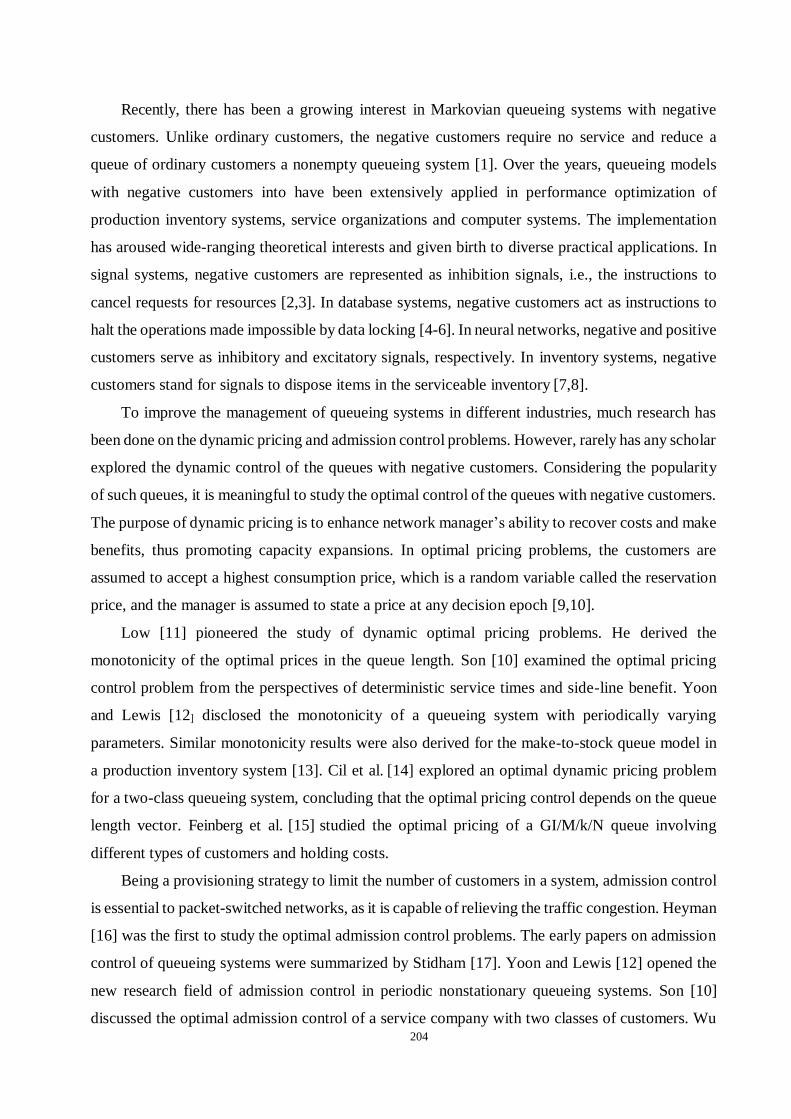
Fig.2. Optimal Threshold and Average Benefit vs. λ- for λ+=0.6, h-=1, c=3
Page 11
213
Fig.3. Optimal Threshold and Average Benefit vs. h for λ+=0.7, λ- =0.5, c=3
Fig.4. Optimal Threshold and Average Benefit vs. c for λ+=0.8, λ- =0.3, h=1
Table 1 depicts the relationship between the optimal pricing and system state. As shown in the
table, the optimal pricing r*(x) increases with the number of customers in the system x. As the
number grows within certain ranges, the optimal pricing will reach the maximum pricing r*(x)=6
and remain the same. The phenomena are consistent with the reality and easy to explain. For
example, when the number of customers becomes sufficiently large in the system, the holding cost
will grow, forcing the manager to propose the maximum pricing and reject the arriving customers.
Figures 1~4 present the numerical results on the response of the optimal policy and average
benefit to the system parameters λ+, λ-, h and c. As shown in Figure 1, the optimal threshold
decreases with the increase of λ+, while the average benefit first increases and then decreases with
the increase of λ+. The increase of the average benefit is attributable to the system welfare brought
by the arriving positive customers, while the decrease of the average benefit is resulted from the
growing number of positive customers, and the ensuing growth in holding cost in a certain interval.
Page 12
214
Figure 2 shows the effect of rate λ-on the optimal threshold and average benefit. It can be seen that
the optimal threshold increases with parameter λ-, and the average benefits grows with ξ but at a
slower rate. As can be seen from Figures 3 and 4, the optimal threshold decreases with the increase
of h, while the average benefit falls with the increase of either h or c. Moreover, all the values of
the optimal thresholds exhibit a staircase-like monotonous pattern, indicating that the optimal
threshold is not affected by the minor changes of system parameters.
Conclusion
This paper digs into the optimal dynamic pricing and admission control policies to maximize
the average benefit in a Markovian queue with negative customers. The negative customers, as a
type of item removal signals, are frequently employed to solve the congestion problem in the
production inventory system. Treating the problem as a Markov decision process, the author
derived the monotonicity of the optimal pricing policy, proved the optimal admission policy as a
threshold policy after analysing the properties of the value function, and discovered the
monotonicity of the optimal thresholds to some system parameters through comparisons. Moreover,
the Howard’s iteration algorithm was adopted for the numerical experiments, which were designed
to reveal the behaviours of optimal policies were studied under different values of system
parameters. The proposed method is applicable to a wide range of models, including the optimal
maintenance and production policies in the production system, and the optimal routing, scheduling
and production policies in the management system.
Further investigation is needed to apply the results to simulate more complex systems. For example,
the proposed model could be extended to study the optimal control problem in the queues with disaster,
or implemented in systems of which the service time obeys the general distribution of the embedded
Markov process and semi-Markov process. Furthermore, the optimal control of the model may be
combined with the uncertainties to provide more accurate information to the manager. Such uncertainties
include randomness and fuzziness, which are commonplace in actual product inventory systems.
Appendix
The proof of Lemma 3.1 (1)
Proof. To prove the decreasing property of operator TP, let r* be the optimal price for the state x+1.
Then we show that pricing operator TP preserves the decreasing property of v(x)in x. From the
definition of the pricing operator TP, we get
Page 13
215
The first inequality follows by taking a potentially suboptimal action in state x and the second
inequality is based on the decreasing property of v(x) in x. The equality follows by the definition
of r*. Hence, we have TPv(x)≥TPv(x+1).
To prove the concavity of operator TP, let r1, r2 and r3 be the optimal prices for the states x, x+1
and x+2. Then we show that pricing operator TP preserves the concavity of v(x) in x. From the
definition of the pricing operator TP, we get
The first equality is based on the definition of the pricing operator and the inequality follows
by taking a potentially suboptimal action in state x+1.
The first equality is based on the definition of the pricing operator and the inequality follows
by taking a potentially suboptimal action in state x+1 and the second equality is based on arranging
the terms. Because of the concavity property of v(x), we have 2v(x)-v(x+1)-v(x+2)≥0 and 2v(x+1)-
v(x+2)-v(x+3)≥0. Hence, we get 2TPv(x)-TPv(x+1)-TPv(x+2) ≥0.
To prove the convexity of operator TP, let be the optimal price for the state x. Then we show
that TP preserves the convexity of v(x) in x. From the definition of TP, we get
Page 14
216
The first inequality follows by taking a potentially suboptimal action in states x-1 and x+1.
The equality is based on arranging the terms and the second inequality is based on the assumption.
The proof of Lemma 3.1 (2)
Proof. To prove the decreasing property of operatorTA, we can get it from the decreasing
property of v(x) and the definition of the admission operator TA. We omit the details here. To prove
the concavity of operator TA, from the definition of operator TA, we get
Because of the concavity property of v(x), the above equation has four cases:
Due to the concavity of v(x), the cases (a) and (b) hold. Since we have v(x-1)-c≥v(x) in case
(c) and v(x-1)-c≥v(x) in case (d), the cases (c) and (d) hold. Therefore we get 2TA v(x)- TA v(x+1)-
TA v(x-1) ≥0, i.e., the operator TA preserves the concavity of v(x).
The proof of Lemma 3.2
Proof. To prove Lemma 3.2 (1), from Lemma 3.1, we know that 2v(x)-v(x+1)-v(x-1)≥0, which
implies that the function H(x) is increasing for all xE.
To prove Lemma 3.2 (2), the proof is by induction on n in vn(x). Define v0(x)=-cx for all states
xE. This function satisfies the property vn(0)-vn(1)-c≥0. Now, we assume vn(0)-vn(1)-c≥0.One
has to prove that vn+1(x)satisfies the property vn+1(0)-vn+1(1)-c≥0 as well. Let r0, r1 be the optimal
prices for the state 0 and 1, respectively in the model. Based on the equation (3.1), we have:
Page 15
217
Rearranging the terms above, we get
The first in equality follows by taking a potentially suboptimal action in state x and the second
inequality based on the concavity property of v(x), i.e, vn(1)-vn(2) ≥vn(0)-vn(1). The third inequality
follows by the assumption vn(0)-vn(1)-c≥0 and the last inequality based on the conditions h/μ ≥c
and λ++λ-+μ=1. Therefore, we have v(0)-v(1)-c≥0.
The proof of Lemma 3.3
Proof. From the definition of the operators TP and TA, we get that the first order differences
for the operators can be written as follows:
.
In order to prove the properties, we mainly use the fixed point theorem and the iterative
induction method. As the properties have the similar structure, we just consider the case q=λ+ and
the other cases can be proved in this way. We first show that the operators TP and TA preserve the
property∆vλ+
+ε(x)≥∆vλ+(x).i.e ∆TPvλ
++ε(x)≥∆TPvλ
+(x), ∆TAvλ+
+ε(x)≥∆TAvλ+(x).
The proof of the result ∆TAvλ+
+ε(x) ≥ ∆TAvλ+(x) can be found in [12]. Next we will give the
proof of the result ∆TPvλ+
+ε(x)≥∆TPvλ+(x). Let r1 and r2 be the optimal prices for the states x in the
model with λ++ε and x-1 in the model with λ+ respectively. Then we show that pricing operator TP
preserves the property∆vλ+
+ε(x)≥∆vλ+(x). From the definition of the pricing operator TP ,we get
Page 16
218
While the coefficient of the operators TP, TA and the uniformization rate are dependent on the
parameter q when q{λ+, λ-}.We need to show the following property∆TP vλ+ (x)-∆vλ
+(x)≥0.. Let r
be the optimal price for the state x. From the definition of the operator TP and the concavity property
∆v(x)≥∆v(x-1), we have
Based on these properties above, we have the following inequality:
Therefore, we have ∆vλ+
+ε(x)≤∆vλ+(x). Meanwhile, we can get the result ∆vh+ε(x)≤∆vh(x), ∆vλ
-
+ε(x)≤∆vλ-(x). and ∆vc+ε(x)≤∆vc(x) in the same way.
References
1. E. Gelenbe, Product-form queueing networks with negative and positive customers, 1991,
Journal of Applied Probability vol. 28, no. 3, pp. 656-663.
2. J.R. Artalejo, G-networks: A versatile approach for work removal in queueing networks,
2000, European Journal of Operational Research, vol. 126, no. 2, pp. 233-249.
3. C.S. Kim, V.I. Klimenok, D. Orlovskii, Multi-server queueing system with a batch Marconian
Page 17
219
arrival process and negative customers, 2006, Automation and Remote Control, vol.67, no.12,
pp. 1958-1973.
4. I. Atencia, P. Moreno, A single-server g-queue in discrete-time with geometrical arrival and
service process, 2005, Performance Evaluation, vol. 59, no.1, pp. 85-97.
5. A. Pechinkin, Markov queueing system with finite buffer and negative customers affecting the
queue end, 2007, Automation and Remote Control, vol. 68, no. 6, pp. 1104-1117.
6. C.H. Wu, W.C. Chien, Y.T. Chuang, Y.C. Cheng, Multiple product admission control in
semiconductor manufacturing systems with process queue time (PQT) constraints, 2016
Computers & Industrial Engineering vol. 99, pp. 347-363.
7. P.V. Laxmi, M. Soujanya, K. Jyothsna, An inventory model with negative customers and
service interruptions, 2016, International Journal of Mathematics in Operational Research,
vol. 9, no. 1, pp. 1-14.
8. M. Soujanya, et.al, Perishable inventory system with service interruptions, Retrial Demands
and Negative Customers, 2015, Applied Mathematics and Computation, vol. 262, pp. 102-
110.
9. B. E. Cil, F. Karaesmen, E.L. Ormeci, Dynamic pricing and scheduling in a multi-class single-
server queueing system, 2011, Queueing Systems, vol. 67, no. 4, pp. 305-331.
10. J.D. Son, Optimal admission and pricing control problem with deterministic service times
and side line profit, 2008, Queueing Systems, vol. 60, no. 1-2, pp. 71-85.
11. D.W. Low, Optimal dynamic pricing policies for an m/m/s queue, 1974, Operations Research,
vol. 22, no. 3, pp. 545-561.
12. S. Yoon, M.E. Lewis, Optimal pricing and admission control in a queueing system with
periodically varying parameters, 2004, Queueing Systems, vol. 47, no. 3, pp. 177-199.
13. J, Gayon, I. Degirmenci, F. Karaesmen, E.L. Ormeci, Dynamic pricing and replenishment in
a production/inventory system with Markov-modulated demand, 2004, Probability in
Engineering and Informational Sciences.
14. B. Cil.E. E.L. O¨rmeci, F. Karaesmen, Effects of system parameters on the optimal policy
structure in a class of queueing control problems, 2009, Queueing Systems, vol. 61, no. 4, pp.
273-304.
15. E.A. Feinberg, F. Yang, Optimal pricing for a GI/M/K/N with several customer types and
holding costs, 2016, Queueing Systems, vol. 82, no. 1-2, pp. 103-120.
16. D.P. Heyman, Optimal operating policies for M/G/1 queuing systems, 1968, Operations
Research, vol. 16, no. 2, pp. 362-382.
Page 18
220
17. J.S. Stidham, Optimal control of admission to a queueing system, 1985, Automatic Control,
IEEE Transactions on, vol. 30, no. 8, pp. 705-713.
18. J. Wu, Z. Liu, G. Yang, Analysis of the finite source MAP/PH/N retrial g-queue operating in
a random environment, 2011, Applied Mathematical Modelling, vol. 35, no. 3, pp. 1184-1193.
19. G. Koole, Monotonicity in Markov reward and decision chains, 2007, Theory and applications.
20. K.Y. Lin, S.M. Ross, Optimal admission control for a single-server loss queue, 2004, Journal
of Applied Probability, pp. 535-546.
21. M.L. Puterman, Markov decision processes: discrete stochastic dynamic programming, 2014,
John Wiley & Sons.
22. H.C. Tijms, Stochastic models: An algorithmic approach, 1994, John Wiley & Sons.
23. Y. Aviv, A. Federgruen, The value iteration method for countable state Markov decision
processes, 1999, Operations Research Letters, vol. 24, no. 5, pp. 223-234.
24. L.I. Sennott, Stochastic dynamic programming and the control of queueing systems, 2009,
vol. 504, John Wiley & Sons.
25. S. Benjaafar, J. P. Gayon, S. Tepe, Optimal control of a production–inventory system with
customer impatience, 2010, Operations Research Letters, vol. 38, no. 4, pp. 267-272.