Optimal pricing of transmission services: application to large power systems

E.D. Farmer B.L.P.P. Perera B.J. Cory

Indexing terms: Large power systems, Optimal pricing, Transmission seruices

Abstract: The paper describes the application of a previously reported [4] optimal transmission pricing method to a large power system. The transmission prices are determined by a global benefit optimisation algorithm that allocates both capacity and operational costs on a time-of-use basis. It is shown that optimal prices may be derived using a conventional mathematical pro- gramming algorithm and results are presented in relation to the IEEE 24 bus test network. A particular feature of the present method is the inclusion of both system security and energy transportation costs. This is achieved by a special- ised technique for iterating between benefit maxi- misation and a system security assessment. Results presented illustrate time-of-use transmission tariffs, together with the variation of capacity costs with system security standards.

1 Introduction

The pricing of transmission services based on the short run marginal cost (SRMC) of supplying electricity at a given node was first proposed by Schweppe et al. [l] and then further developed [2, 31. The SRMC based pricing does have two major weaknesses as an efficient pricing strategy for the use of transmission services. First, the SRMC pricing of network services tends to reward the network utility when the network performance deterio- rates (e.g. by increased losses and congestion), which creates perverse incentives for the network utility regard- ing new investments and maintenance practices. Sec- ondly, in actual systems, because of the existence of the important effects of economies of scale, reliability con- straints and other deviations from ideal conditions, the network revenue often falls significantly short of recov- ering the total cost for use of the network.

A novel approach has been proposed by Farmer et al. [4] that alleviates the inherent shortcomings of SRMC based pricing while maintaining the economic efficiency of the price signals. The approach adopted utilises con- ventional economic analysis [SI by deriving the ‘demand for transmission capacity’ in relation to the prices assign- ed to the circuit flows plus the economic benefit attribut-

0 IEE, 1995 Paper 1753C (W), received 10th November 1994 The authors are with the Department of Electrical and Electronics Engineering, Imperial College of Science Medicine and Technology, London SW7 ZBT, United Kingdom

IEE Proc.-Genm. Transm. Distrib., Vol. 142, No. 3, May I995

able to the transmission service provided. The optimum transmission circuit flows and circuit capacities are derived by maximising this benefit function subject to operational constraints. The annuitised capacity cost of the transmission system is optimally allocated among the different participants.

In this paper, this pricing strategy is further improved by incorporating a proper security analysis to evaluate the optimum circuit capacities. The proposed method has been implemented for the IEEE reliability test system ~ 7 1 .

2

The proposed method consists of two stages. The first stage is to determine the ‘inverse demand function’ for the transmission services by maximising the net benefit derived by the users from utilising these services. The ‘consumer net benefit’ can be defined as the total benefit minus the price paid by the users for use of transmission services. The transmission utility or benefit function can then be defined as the sum of the generation cost reduction and the value of the reduced unserved demand. If Ck(gk) denotes the cost of generation power gk at node k, and if Gk,,, is the capacity available, the consumer benefit or utility function is given by

Formulation of optimal pricing problem

where

The generation vector g may be derived from the network flows x and the demand L using the network nodal balance relations obtained from Kirchhoffs laws

(3) g = L + A‘x + 4.4

The financial support of the National Grid Company plc, UK, is gratefully acknowledged in the pursuance of this research. Support by the Presidential Trust Fund of Sri Lanka and the Edmund Davis Scholarship of the University of London for B.L.P.P. Perera is also gratefully acknowledged.

263

where a(x) is half the sum of the losses of all the circuits connected to node n, and A is the branch-nodeincidence matrix. Using the nodal power balance relation (eqn. 3), the benefit function (eqn. 2) may be expressed explicitly in terms of the transmission flows x as

V(x) = n [ L + A'x + 4 x ) ] (4) The nodal power injections have to satisfy the constraints imposed by the output limits of the generators connected at each node. These constraints are given by

(5)

In the case of a DC load flow model of the power network, the branch flows x may not be assigned arbi- trarily, but must satisfy a B - N + 1 dimensional set of voltage mesh conditions for which

0 < L + A'x + 44 < c,,

M t Z b x = 0 (6)

where M is the branch incidence matrix for a set of basic meshes and Z b is the diagonal matrix of the branch series impedance. The constraints (eqns. 5 and 6) may be. added to the objective function with the associated Lagrange multipliers to obtain the transmission utility function:

transmission utility:

It is evident that the transmission utility function U T constitutes a true consumer benefit function as used in conventional economic analysis. It follows that, for a specific set of transmission prices, p the consumer net benefit takes the form:

(8) consumer net benefit: C N B = U T [ x ] - #x

Given the prices p, the consumer chooses the flows to maximise his net benefit C N B (subject to the constraints 5 and 6 implied in the transmission utility function UT). This results in

(9)

The next step is to determine the optimum power flows that maximise the global benefit for use of the transmis- sion service. The global net benefit of transmission usage is the benefit summed over the tariffing period minus the cost of providing the transmission service. A tariffing period T is considered, for which the load duration curve is TG(x) and the load curve is divided into a number of time slots t = 1, 2, . . . , T. The transmission system costs can be divided into two broad categories. These are (i) variable operating costs

&,{xb(t)} associated with the circuit flows xb(t) on circuit b at time t. These include all flow dependent operating and maintenance costs, but exclude trans- mission losses.

(i) capacity costs K~ per unit capacity for circuit route b. This is the annuitised return on invested capital required over the tariffing period T, for each economically justified circuit b.

inoerse demand function: p = grad { U T @ ) } .r

The maximisation of the net benefit may be expressed as

maximise NB[x(t) , X,]

264

subject to fb 1 xb(t) I < xb, rrmx Vb, t (1 1) The security factor f b is introduced to incorporate the cost of transmission capacity required to ensure enough transmission capacity for a defined set of contingencies. The evaluation of a consistent set of security factors is described in the next Section. The optimality condition with respect to xb(t) requires

aUT ag --fbAb(t) = 0 axb(t)

where Ab(t) is the Lagrange multiplier on the constraint (eqn. 11). The transmission price is given by the deriv- ative of the transmission utility function (i.e. eqn. 7) as

The capacity costs are allocated only to the periods where the capacity constraints are active. The flow dependent variable costs are ignored in the implementa- tion, and the expression for optimum transmission prices, given by eqn. 13, is simplified to

P b ( d = +fb Ab(t) (14) The obvious choice to value the transmission losses is the system marginal price given by the shadow cost on the system load balance constraint. As the system load balance constraint is not explicitly considered in the for- mulation explained in the previous Section, the gener- ation cost of the marginal generator for each demand period can be used to evaluate the value of the transmis- sion losses. If there are several marginal generators at a given period, due to the presence of transmission con- traints, then the weighted average of generation cost of these generators is used with their output being the weighting factor. Then the total value of transmission losses is given by

T B T L = c M P , [Rbxb(t)*]

t = l b = 1

where M P , is the weighted generation cost of marginal generators in period t, and Rb is the resistance of branch b.

The transmission loss component of transmissionprice is evaluated as the marginal cost of transmission losses with respect to circuit flows. The total transmission circuit price may be written as

Pb(t) = p'b(t) + P i ( t )

where pi(t) and pk(t) are the capacity and loss component of the transmission prices. In particular,

(16)

The security factors and the optimum transmission capacities for the IEEE reliability Test system (i.e. Fig. 1 and data in the Appendix) are determined by progres- sively considering the three types of contingencies. The annuitised capacity cost is taken as 30.0 €/MW km as this value corresponds to the value used by National Grid Company UK in the ICRP pricing study [SI. Fig. 2 shows the power flows for the period 10. Although period 10 corresponds to the system peak demand, only about

a T L pk(t) = - = 2MPt R , xb(t)

axb(t)

1EE Proc.-Gew. Transm Distrib., Vol. 142, No. 3, May 1995

one-third of the transmission circuits are constrained in this period, because almost all the generators except expensive gas turbines (i.e. generators ‘a’ and ‘c’) are called upon to generate in this period. The resulting gen- eration profile relieves most of the transmission con- straints except in the circuits used to supply load centres such as circuits 10, 11, 17, 18 and 20. The double circuit pairs ‘C’, ‘A’ and ‘ B are also constrained in this period as they are used to supply the relatively high demand in buses ‘18, ‘20’ and ‘W, respectively.

@ qen k Q a e n 1

\, geno,b 9enc.d gen e

IEEE 24 bus reliability test system

. Fig. 1

Fig. 2 period IO

-0- powernow

Optimum power flows and transmission capacity prices for

H capacity price

3 Transmission security factors

The security costs on a transmission system may be evaluated in terms of transmission security factors that relate power flows following system faults to those on the intact power network. For this purpose, the projected tariffing period T is divided into a number of time slots t = 1, 2, ..., T that correspond to the division of the demand curve into block loads or to a discretisation of the load duration curve (LDC) over the tariffing period. Maximum flows for the intact network (i.e. max, {x,(t)})

IEE Proc.-Gener. Transm. Distrib., Vol. 142, No. 3, May I995

are initially derived with an assumed set of security factors using the benefit maximisation algorithm explained in the previous Section. In relation to the defined set of contingencies, load flow calculations may be used to determine, for each circuit, the contingent power flow t,(t) as explained in the next Section. Then the security factorf, is defined by

maximumover { , } fb = all contingencies max iXb(t )} (17)

Thus the security factorf, is the ratio of power flow fol- lowing the worst contingency i , ( t ) to the maximum flow, max, {x,(t)} , on the intact network. These factors do not assume that the worst contingencies are coincident with the system peak demand, asfb is determined over each of the tariffing periods considered. For any circuit b, it is evident that a maximum flow, max, {x,(t)} on the intact network necessitates the construction of a total circuit capacity f a max, {x,(t)} to ensure system security. The security factors are updated with the values determined in eqn. 17 and used in determining the circuit capacities and intact network flows in the benefit maximisation process. This process is repeated until a secure set of transmission capacities is obtained with respect to the contingencies considered. This requires the worst contin- gent flow to be less than the circuit capacity determined by

It was observed that, if the security factorf, is relatively large for a particular circuit (i.e. greater than 3.0), the resulting maximum circuit flow in that circuit in the sub- sequent iteration becomes progressively smaller. This would result in even larger security factors in the sub- sequent iterations. For this reason the security factors were divided into two components (i.e. multiplicative and additive) if greater than 3.0. This division can be expressed as

iff, < 3.0 f r = f,, f; = 0.0

iff, > 3.0 fr = 3.0 and

where fr and f; are the multiplicative and the additive components of the security factor. The circuit capacity constraint (eqn. 11) in the benefit maximisation algorithm is altered to accommodate the split security factors as

xb, IMX - 1 f ; x b ( t ) I kf; (20) The transmission circuit capacities are determined so as to provide enough capacity in the event of the set of con- tingencies given in Sections 3.1 and 3.2.

3.1 Single and double circuit outages For transmission line or transformer outage contin- gencies, it is assumed that the input (is. generation and demand) load flow variables remain unchanged. This means that specified real and reactive loads, together with real power generation and generator bus voltages, will remain constant before and after the outage. The contingent power flows in the event of transmission circuit outages are evaluated using ‘outage distribution factors’ as defined in [8] given by

265

where

d,,,, I = outage distribution factor for circuit m

x,,,(t), x,(t) = prefault power flows in circuits m and n,

i,,,, .(t) = postfault power flow in circuit m after the

If the prefault power flows are known for the circuits m and n the post fault power flows can be readily computed as

with respect to outage in circuit n

respectively

outage in circuit n.

= x d t ) + 4, I XAt) (22)

32 Generator outages Because of the resultant drop in frequency due to gener- ator outages, the power output of other generators is assumed to be automatically adjusted through automatic generation control (AGC). The new generator outputs may not be optimal from the economic point of view. Subsequently, the generators are redispatched to achieve the minimum cost generation. It is assumed that the orig- inal generator dispatch would be modified with minimum incremental cost to pick up the load served by the outaged generator. This problem may be formulated as

G

minimise 1 cj Ag;(t) (23)

subject to Ag;(t) = g&) (24)

+ s,44 < Gj, mx '0, j f n (25)

j = 1 j # n

G

j = 1 j#n

where

Agy(t)= the change in the power output of jth gener- ator after the nth generator is tripped

g,(t) = the prefault power output of the jth generator G , IMx = the maximum generation capacity of the jth

cj = the cost of generation of the jth generator

The constraint (eqn. 24) ensures the power balance when the nth generator is tripped, but the change in the trans- mission losses due to the redistribution of power flows is ignored at this stage. The constraint (eqn. 25) ensures that the generator outputs for the postfault dispatch are within the generator capacity limits. The postfault power flow on the mth circuit after the nth generator is tripped e(t) may be determined using the sensitivity matrix [HJ reflecting circuit flows to nodal power injections derived in [SI as

(26)

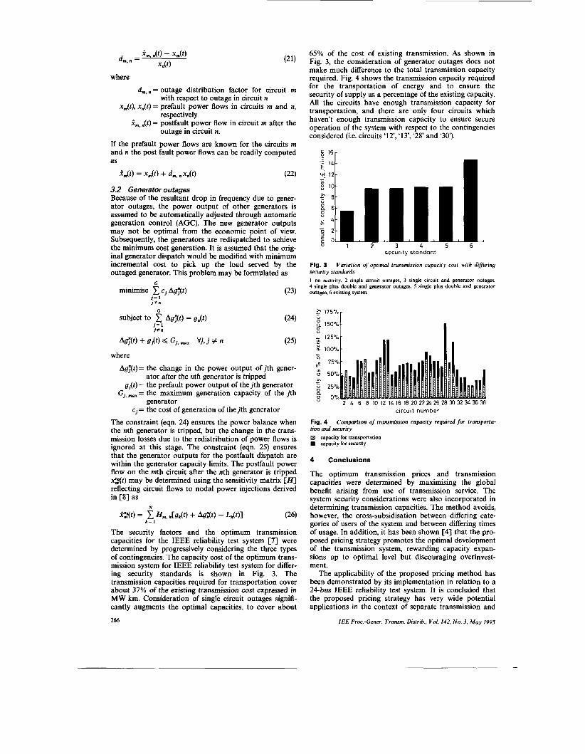
The security factors and the optimum transmission capacities for the IEEE reliability test system [7] were determined by progressively considering the three types of contingencies. The capacity cost of the optimum trans- mission system for IEEE reliability test system for differ- ing security standards is shown in Fig. 3. The transmission capacities required for transportation cover about 37% of the existing transmission cost expressed in MW km. Consideration of single circuit outages signifi- cantly augments the optimal capacities, to cover about

generator

N

az(t) = 1 Hm, t [ g d t ) + A d ( t ) - Lk(t) l k = l

266

- - - 14- E. w. 12- -

65% of the cost of existing transmission. As shown in Fig. 3, the consideration of generator outages does not make much difference to the total transmission capacity required. Fig. 4 shows the transmission capacity required for the transportation of energy and to ensure the security of supply as a percentage of the existing capacity. All the circuits have enough transmission capacity for transportation, and there are only four circuits which haven't enough transmission capacity to ensure secure operation of the system with respect to the contingencies considered (i.e. circuits 'U, '13', '28' and '30).

securlty standard

Fig. 3 Variation of optimal transmission capacity cost with differing security standards I no security, 2 single circuit outages, 3 single clrcuit and generator outages, 4 single plus double and generator outages, 5 single plus double and generator outages, 6 existing system

2' 175%

150% B

clrcult number

Comparison of transmission capacity required for transporta- Fig. 4 tion and security

capacity for transpatation capacity for security

4 Conclusions

The optimum transmission prices and transmission capacities were determined by maximising the global benefit arising from use of transmission service. The system security considerations were also incorporated in determining transmission capacities. The method avoids, however, the cross-subsidisation between differing cate- gories of users of the system and between differing times of usage. In addition, it has been shown [4] that the pro- posed pricing strategy promotes the optimal development of the transmission system, rewarding capacity expan- sions up to optimal level but discouraging overinvest- ment.

The applicability of the proposed pricing method has been demonstrated by its implementation in relation to a 24-bus IEEE reliability test system. It is concluded that the proposed pricing strategy has very wide potential applications in the context of separate transmission and

IEE Proc.-Gem. Transm Distrib., Vol. 142, No. 3, May 1995

distribution pricing, for wheeling transactions between geographically separate utilities, for third party and open access to the transmission system and for common carrier charging. The derived prices send optimal cost messages to all participants and to the transmission utility. The method results in stable and transparent prices, so promoting efficient business planning by all supply system participants.

5 References

1 CARAMANIS, M., BOHN, R., and SCHWEPPE, F.C.: 'The costs of wheeling and optimal wheeling rates', IEEE Tram., 1986, T-PWRS, pp. 63-73

2 SCHWEPPE, F.C., CARAMANIS, M.C., TABORS, R.D., and BO", R.E.: 'Spot pricing of electricity' (Kluwer Academic Publi- shers, 1988)

3 PEREZ-ARIAGA, I.J., RUBIO, F.J., PURETA, J.F., ARCELUZ, J., and MARIN, J.: 'Marginal pricing of transmission services: an analysis of cost recovery'. IEEE summer meeting 1994,94 SM 528-0 PWRS

4 FARMER, E.D., PERERA, P.P., and CORY, B.J.: 'Optimal pricing of transmission services', IEE h o c . GTD, 1995,142, (l), pp. 1-8

5 PRESSMAN, I.: 'Mathematical formulation of the peak load pricing problem', Bell J . Econ., 1970,1, (2). pp. 305-326

6 DUNNElT, R.M., CALVIOU, M.C., and PLUMFTRE, P.H.: 'Charging for use of a transmission by marginal cost methods'. 11th power system computation conference, Avignon, France, 1993

7 RELIABILITY TEST SYSTEM TASK FORCE O F THE APPLI- CATION OF PROBABILITY METHODS SUBCOMMITTEE: 'IEEE reliability test system', IEEE Tram., 1979, PAS-98, pp. 2047- 2n54

Table 2: Load duration curve sampling data for IEEE 24 bus reliability test system

Demand Load level as % Number period of peak demand of hours

1 0.43 895 2 0.47 842 3 0.51 874 4 0.55 894 5 0.61 897 6 0.66 899 7 0.70 888 8 0.76 881 9 0.82 81 1 10 1 .o 856

Table3: Generator data for IEEE 24 bus reliability test svstem

Generator Generator Number Maximum Cost name bus of units capacitv

'a' '1 ' 2 ' b '1 ' 2 'C' '2 2 'd' '2 2 '0' '7' 3 'f' '1 3 3 'g' '1 5 5 'h' '1 6 1 7' '1 5 1 'i' '1 8 1

MW f/MWh 20 50.0 76 15.3 20 50.0 20 15.3 100 24.03 197 23.33 12 29.1 155 12.44 155 12.44 400 6.3 _.. .

8 WOOD, A.J., and WOLLENBERG, B.F.: 'Power generation, oper- 'k' '21, 1 400 6.3 ation and control' (John Wiley & Sons, 1984) 'I' '22 5 60 0.0

'm' '23 2 155 12.44 'n' '23 1 350 12.1

6 Appendix: Data for IEEE 24 bus test system

Table 1 : Demand data for IEEE 24 bus reliability test system

Bus name Peak demand

Table 4: Circuit data (continued overleaf)

MW '1 ' 108 '2 97 '3 180 '4 74 '5 71 '6 136 '7' 125 ' 8 171 '9 175 '1 0 195 '1 1' 0.0 '1 2 0.0 '1 3 265 '1 4 194 '1 5 31 7 '1 6 100 '1 7 0.0 '1 8 333 '1 9 181 '20 128 '21 ' 0.0 '22 0.0 '23 0.0 '24' nn

IEE Proc.-Gew. Transm Distrib., Vol. 142, No. 3, May 1995 267

268

Table 4: Circuit data for IEEE 24 bus reliability test system

Circuit Starting Terminating Circuit Resistance Reactance capacity number bus bus length

1 2 3 4 5 6 7 8 9 10 11 12 13 14 15 16 17 18 19 20 21 22 23 24 25 26 27 28 29 30 31 32 33 34 35 36 37 38

'1 ' '1 ' '1 ' '2 ' 2 '3 '3 '4 ' 5 ' 6 '7' '8' ' 8 ' 9 ' 9 '1 0 '1 0 71 ' '11' '1 2 '1 2 '1 3 '1 4 '1 5 '1 5 '1 5' '1 5' '1 6' '1 6' '1 7. '1 7, '1 8 '1 ti '1 9 '1 9 '20 '20 '21 '

km '2 3 ' 3 55 ' 5 22 '4 33 ,6 50 '9' 31 '24 50 '9' 27 '1 0 23 '1 0 16 'ti 16 ' 9 43

'1 1 50 '1 2 50 '11' 50 '1 2 50 '1 3 33 '1 4 29 '1 3 33 '23 67 '23 60 '1 6' 27 '1 6' 12 '21 ' 34 '21 ' 34 '24 36 '1 7' 18 '1 9 16 '1 8 10 '22 73 '21 ' 18 '21 ' 18 '20 27.5

'1 0; 43

'20 27.5 '23 15 '23 15

p.u.on MVA base p.u.on MVAbase MW 0.0026 0.01 39 175 ~~ ~

0.0546 0.0218 0.0328 0.0497 0.0308 0.0023 0.0268 0.0228 0.01 39 0.01 59 0.0427 0.0427 0.0023 0.0023 0.0023 0.0023 0.0061 0.0054 0.0061 0.01 24 0.01 11 0.005 0.0022 0.0063 0.0063 0.0067 0.0033 0.003 0.001 8 0.01 35 0.0033 0.0033 0.0051 0.0051 0.0028 0.0028

0.21 12 0.0845 0.1 267 0.01 92 0.119 0.0839 0.1 037 0.0883 0.0605 0.061 4 0.1 651 0.1 651 0.0839 0.0839 0.0839 0.0839 0.0476 0.041 8 0.0476 0.0966 0.0865 0.0389 0.01 73 0.049 0.049 0.051 9 0.0259 0.0231 0.01 44 0.1 053 0.0259 0.0259 0.0396 0.0396 0.021 6 0.021 6

175 175 175 175 175 400 175 175 175 175 175 175 400 400 400 400 500 500 500 500 500 500 500 500 500 500 500 500 500 500 500 500 500 500 500 500

'22 47 0.0087 0.0678 500

I E E Proc.-Gener. Transm. Disrrib., Vol. 142, No. 3, M a y 1995