SANDIA REPORT SAND2010-6237 Unlimited Release Printed September 2010 Optimal Recovery Sequencing for Critical Infrastructure Resilience Assessment Eric D. Vugrin, Mark A. Turnquist, and Nathanael J. K. Brown Prepared by Sandia National Laboratories Albuquerque, New Mexico 87185 and Livermore, California 94550 Sandia National Laboratories is a multi-program laboratory managed and operated by Sandia Corporation, a wholly owned subsidiary of Lockheed Martin Corporation, for the U.S. Department of Energy's National Nuclear Security Administration under contract DE-AC04-94AL85000. Approved for public release; further dissemination unlimited.
Transcript
SANDIA REPORT SAND2010-6237 Unlimited Release Printed September 2010
Optimal Recovery Sequencing for Critical Infrastructure Resilience Assessment Eric D. Vugrin, Mark A. Turnquist, and Nathanael J. K. Brown Prepared by Sandia National Laboratories Albuquerque, New Mexico 87185 and Livermore, California 94550
Sandia National Laboratories is a multi-program laboratory managed and operated by Sandia Corporation, a wholly owned subsidiary of Lockheed Martin Corporation, for the U.S. Department of Energy's National Nuclear Security Administration under contract DE-AC04-94AL85000. Approved for public release; further dissemination unlimited.
2
Issued by Sandia National Laboratories, operated for the United States Department of Energy by Sandia Corporation. NOTICE: This report was prepared as an account of work sponsored by an agency of the United States Government. Neither the United States Government, nor any agency thereof, nor any of their employees, nor any of their contractors, subcontractors, or their employees, make any warranty, express or implied, or assume any legal liability or responsibility for the accuracy, completeness, or usefulness of any information, apparatus, product, or process disclosed, or represent that its use would not infringe privately owned rights. Reference herein to any specific commercial product, process, or service by trade name, trademark, manufacturer, or otherwise, does not necessarily constitute or imply its endorsement, recommendation, or favoring by the United States Government, any agency thereof, or any of their contractors or subcontractors. The views and opinions expressed herein do not necessarily state or reflect those of the United States Government, any agency thereof, or any of their contractors. Printed in the United States of America. This report has been reproduced directly from the best available copy. Available to DOE and DOE contractors from U.S. Department of Energy Office of Scientific and Technical Information P.O. Box 62 Oak Ridge, TN 37831 Telephone: (865) 576-8401 Facsimile: (865) 576-5728 E-Mail: [email protected] Online ordering: http://www.osti.gov/bridge Available to the public from U.S. Department of Commerce National Technical Information Service 5285 Port Royal Rd. Springfield, VA 22161 Telephone: (800) 553-6847 Facsimile: (703) 605-6900 E-Mail: [email protected] Online order: http://www.ntis.gov/help/ordermethods.asp?loc=7-4-0#online
3
SAND2010-6237 Unlimited Release
Printed September 2010
Optimal Recovery Sequencing for Critical Infrastructure Resilience Assessment
Eric D. Vugrin Infrastructure and Economic Systems Analysis Department
Sandia National Laboratories P.O. Box 5800
Albuquerque, New Mexico 87185-MS1138
Mark A. Turnquist School of Civil and Environmental Engineering
Cornell University 220 Hollister Hall Ithaca, NY 14853
Nathanael J. K. Brown
Operations Research and Knowledge Systems Sandia National Laboratories
P.O. Box 5800 Albuquerque, New Mexico 87185-MS1138
Abstract
Critical infrastructure resilience has become a national priority for the U. S. Department of Homeland Security. System resilience has been studied for several decades in many different disciplines, but no standards or unifying methods exist for critical infrastructure resilience analysis. This report documents the results of a late-start Laboratory Directed Research and Development (LDRD) project that investigated the identification of optimal recovery strategies that maximize resilience. To this goal, we formulate a bi-level optimization problem for infrastructure network models. In the “inner” problem, we solve for network flows, and we use the “outer” problem to identify the optimal recovery modes and sequences. We draw from the literature of multi-mode project scheduling problems to create an effective solution strategy for the resilience optimization model. We demonstrate the application of this approach to a set of network models, including a national railroad model and a supply chain for Army munitions production.
4
ACKNOWLEDGMENTS The authors would like to thank Dean Jones and Orr Bernstein, Sandia National Laboratories, for providing technical guidance for the R-NAS model. Additionally, Kevin Stamber, Sandia Nation Laboratories; Bill Fogleman and Anna Weddington, GRIT; Michael Mohr and Matthew Nelson of Joint Munitions Command-Industrial Base; James Uribe, Chief of Industrial Preparedness, U.S. Army Material Command; and Al Galonski, Chief of Ammunition Logistics Division, Project Director Joint Service, Program Executive Office Ammunition were critical to providing data and systems knowledge for the munitions supply chain model development. We appreciate the efforts of James Shields, SES, Deputy Program Executive Officer Ammunition, and Wimpy D. Pybus, SES, Deputy Assistant Secretary of the Army, Acquisition Policy and Logistics to identify the munitions supply chain for a case study and for enabling our efforts to model that system. Finally, we would like to thank Dan Rondeau, J. R. Russell, Russ Skocypec, Ray Trechter, Lillian Snyder, and Steve Kleban for recognizing the need to continue basic mathematics research in the support of resilience initiatives. Their programmatic support is greatly appreciated. This work was supported by Laboratory Directed Research and Development funding from Sandia National Laboratories.
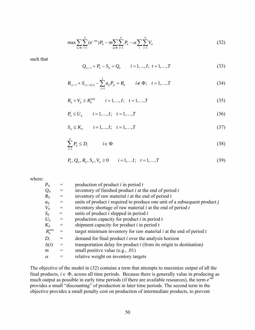
5
CONTENTS
1. Introduction and Background .................................................................................................... 9 1.1. Current Assessment Methods ......................................................................................... 9 1.2. Project Goals ................................................................................................................. 11
2. Mathematical Formulation ........................................................................................................ 13 2.1. Optimization Problem Formulation .............................................................................. 13 2.2. Solving the Optimization Problem................................................................................ 17
3. Applications and Analyses ........................................................................................................ 29 3.1. Optimal Recovery Sequencing when TRE is Constant ................................................ 29
3.2.1. Problem Formulation ...................................................................................... 29 3.2.3. Solution Methodology .................................................................................... 30 3.2.4. Application and Analysis ............................................................................... 31 3.2.4. Summary ......................................................................................................... 34
3.2. Application to the U.S. Freight Rail Network .............................................................. 35 3.2.1. The Rail Network Model ................................................................................ 38 3.2.2. Computing the SI and TRE Measures ............................................................ 40 3.2.3. Implementation of the Simulated Annealing Algorithm with R-NAS ........... 41 3.2.4. Results of the Analysis.................................................................................... 43
3.3. Dynamic Munitions Supply Chain Example ................................................................ 47 3.3.1 Model Formulation ............................................................................................. 48
4. Summary and Conclusions ....................................................................................................... 55
Appendix A: Additional Details for the Rail Network Resilience Software ............................... 61 Evaluation of RNR Software .................................................................................................. 61 Input Files ............................................................................................................................... 61 Output Files ............................................................................................................................. 61 Object Model of RSW ............................................................................................................ 62 Configuration File ................................................................................................................... 65
Distribution ................................................................................................................................... 70
6
FIGURES
Figure 1. Illustrative Activity-on-arc Project Network. ................................................................ 18 Figure 2. Schedule and Resource Loading Associated with the Sequence ................................... 19 Figure 3. Schedule and Resource Loading Associated with the Sequence ................................... 20 Figure 4. Example Transportation Network. ................................................................................ 20 Figure 5. Trial 1 schedule for example network. .......................................................................... 24 Figure 6. Trial 2 schedule for example network. .......................................................................... 24 Figure 7. Trial 3 schedule for example network. .......................................................................... 25 Figure 8. Trial 4 schedule for example network. .......................................................................... 25 Figure 9. Trial 5 schedule for example network. .......................................................................... 25 Figure 10 . Measurement of SI for the example sequence. ........................................................... 26 Figure 11. Algorithm statement for Boctor’s (1996) implementation of simulation annealing for project scheduling. ........................................................................................................................ 27 Figure 12. Transportation Network (a) nominal state and (b) disrupted state. ............................ 32 Figure 13. Union Pacific traffic density (2007 data). ................................................................... 36 Figure 14. Representation of main lines in the national rail network. ......................................... 38 Figure 15. Transportation Analysis Zones (TAZs) and centroids. .............................................. 39 Figure 16. Locations of other Mississippi River crossings. .......................................................... 43 Figure 17. Optimal restoration schedule for damaged bridges. .................................................... 45 Figure 18. Systemic impact summary for optimal restoration plan. ............................................. 46 Figure 19. Restoration schedule assuming no cooperation among companies. ............................ 47 Figure 20. Systemic impact summary for “independent” restoration plan. .................................. 47 Figure 21. Bill-of-materials (BOM) network representation. ....................................................... 49 Figure 22. Time-space network representation of movements within a supply network. ............ 49 Figure 23. Cumulative production of product 1 after three-week disruption at the beginning of the planning horizon. .................................................................................................................... 52 Figure 24. Cumulative production of product 1 when production of a tier 2 material is constrained. ................................................................................................................................... 53 Figure 25. Cumulative production of product 2 when production of a tier 2 material is constrained. ................................................................................................................................... 53 Figure 26. Cumulative production of product 2 when tier 1 supplier has larger initial raw material inventory. ...................................................................................................................................... 54
7
TABLES
Table 1. Link Characteristics for Example Transportation Network. ........................................... 21 Table 2. Equilibrium flow for nominal (base) case. ..................................................................... 21 Table 3. Equilibrium flow for damaged condition (unmet demand = 200). ................................. 22 Table 4. Parameters for modes of repair on damaged links. ......................................................... 22 Table 5. Sample of repair modes on damaged links for 5 trials. .................................................. 23 Table 6. Equilibrium flow for partially restored condition at time 3 (unmet demand = 200). ..... 26 Table 7. Equilibrium flow for partially restored condition at time 4 (unmet demand = 125). ..... 26 Table 8. Network link characteristics. ......................................................................................... 32 Table 9. Additional network characteristics. ............................................................................... 32 Table 10. Optimal network flows when = 20. ..................................................................... 33 Table 11. Network flows when = 20 and link 1,4 is restored first. ..................................... 33 Table 12. Optimal network flows when = 10, and = 2. .............................................. 34 Table 13. Network flows when = 10, and = 2 and link 1,5 is restored first. .............. 34 Table 14. Summary of daily flow statistics within five-state region. ........................................... 44 Table 15. Summary of daily flow changes within five-state region with all four bridges out of service. .......................................................................................................................................... 44
8
9
1. INTRODUCTION AND BACKGROUND
Historically, U. S. Federal Government policy towards critical infrastructure protection (CIP) has focused on physical protection and asset hardening (e.g., see Reagan, 1982; Clinton, 1998; Bush, 2002; 2003). In recent years, CIP policies have shifted to include critical infrastructure resilience concepts and strategies. Critical infrastructure resilience (CIR) is a concept that describes the ability of infrastructure systems to absorb, adapt, and recover from the effects of a disruptive event while attempting to continue delivery of critical infrastructure services. The federal government has started a coordinated set of government resilience initiatives to begin the process of understanding what features create resilience in critical infrastructure systems. The DHS National Infrastructure Protection Plan (NIPP), in particular, contains explicit language calling for increasing the resilience of the nation’s critical infrastructure. Many of the NIPP sector-specific plans (SSPs) also have broad, if not specific, language that promotes critical infrastructure resilience as a primary objective. For example, in its SSP, the Transportation Security Administration (TSA) made “Enhance the resilience of the transportation system” one of its top three priorities (TSA, 2007). The process of institutionalizing CIR analysis in federal policy faces many challenges. In particular, the lack of standardized CIR definitions and analysis methods must be addressed in order to develop effective CIP policies. 1.1. Current Assessment Methods Holling (1973) provided the first systems level definition of resilience more than 30 years ago. Since that initial definition, many different definitions of resilience have been proposed for use in infrastructure and economic systems analysis (for examples, see Bruneau et al., 2003; Chang and Shinozuka, 2004; Rose and Liao, 2005). These definitions all include some aspect of a system withstanding change due to a disruption or disturbance, whether by reducing the impact of the change, adapting to the change, or recovering from the change. Despite the large number of resilience definitions, few quantitative methods have been proposed for analysis of infrastructure and economics systems. Bruneau et al. (2003) measure seismic resilience loss for communities by integrating the difference between optimal infrastructure quality, i.e., 100 percent, and the degraded infrastructure quality following an earthquake. Chang and Shinozuka (2004) use a probabilistic formulation to estimate a system’s seismic resilience. They compare the decrease in system performance and time to recovery, predicted through a set of Monte Carlo simulations, against pre-defined performance and duration standards. According to this approach, the resilience of the system is the observed probability that both standards are met. Rose and Liao (2005) have developed resilience metrics for economic systems. Rose asserts that the static economic resilience of a system be measured as “the ratio of the avoided drop in [system] output and the maximum potential drop” in system output,. He further asserts that dynamic economic resilience be measured as the cumulative difference between system outputs with and without hastened recovery efforts. Each of these approaches focuses on the impact that a disturbance has on the state of the system or system outputs.
10
In general, these approaches have a common limitation: they do not explicitly consider the important role that recovery processes have in determining system resilience. Specifically,
The effectiveness of the recovery strategy that one selects directly affects the magnitude and duration of system performance impacts. Said differently, the resilience of a system to a particular disruption is a function of the recovery strategy initiated following the occurrence of that event.
Expenditure of resources during the recovery processes could be a significant contributor in the overall impacts and costs resulting from a disruption. Resource requirements for recovery strategies will affect the recovery strategy decision process. Additionally, the amount of resources required for a particular strategy may affect whether that strategy is feasible in a resource constrained environment.
Hence, for these two reasons, we assert that recovery costs must be explicitly accounted for in CIR assessments. Resource allocation can be a critical concern during crisis events, and emergency responders need to decide how limited resources should be spent to minimize deleterious impacts and maximize response efficiencies. Vugrin, et al. (2010) have proposed a resilience assessment framework that expands upon the aforementioned assessment approaches in two key areas. First, Vugrin, et al.’s mathematical formulation for measuring resilience costs is not reliant upon a specific modeling paradigm to represent the system, so it can be generally applied across various infrastructure and economics models. This flexibility is necessary for establishing resilience analysis standards across all CIKR systems. Secondly, it explicitly considers the costs and resources expended during recovery efforts following infrastructure disruptions. Inclusion of recovery costs in resilience evaluations provides a more comprehensive accounting of disruption impacts. This approach also provides a means for assessing feedback loops that include recovery processes and system performance. Vugrin, et al. (2010) define system resilience as follows:
Given the occurrence of a particular disruptive event (or set of events), the resilience of a system to that event (or events) is the ability to efficiently reduce both the magnitude and duration of the deviation from targeted system performance levels.
This definition provides the basis for the measurement of the two primary factors that determine the resilience costs: systemic impact (SI) and total recovery effort (TRE). SI is the impact that a disruption has on system productivity TRE refers to the efficiency with which the system recovers from a disruption. Consider a dynamic system modeled as follows:
, ,y t F X U t D t t (1)
where X is a state vector with dependence on the control term U and the disturbance D: U is a time-dependent control vector representing the means by which the system
recovers, i.e., U is the recovery effort; D represents a time-dependent, piece-wise continuous, disturbance forcing term.
11
y is the vector of system outputs under disturbance D, and is obtained by calculation of the function F.
Let z be an exogenous reference signal that represents the time-dependent, targeted system performance level. Vugrin, et al. (2009) calculate SI and TRE as follows:
0
( ) ( ) ,tf
T
t
SI q z t y t dt (2)
tf
t
T dtturTRE0
. (3)
where t0 > 0 is the time at which the disturbance initiates and tf is the time at which recovery is considered complete. The vectors q and r consist of sets of weighting factors that are used to calculate costs of decreased system performance and resource expenditures, respectively. Since X and y are dependent upon U; Vugrin, et al. (2010) define two types of resilience cost measurements: Recovery dependent resilience costs are those costs resulting from a particular recovery strategy, and they are calculated according to (4).
0
( 0 , , )
( )tf
T
t
SI TRERDR X t D U
q z t dt
(4)
The denominator in (4) is a normalizing term that permits comparison of RDR values for systems of varying magnitudes. When they exist, Vugrin et al. use the term optimal resilience costs, OR, to refer to the resilience costs that are minimized by an optimal recovery strategy. These costs are calculated as
0
( 0 , ) min
( )U tf
T
t
SI TREOR X t D
q z t dt
(5)
1.2. Project Goals Vugrin, et al.’s (2010) resilience cost approach lends itself nicely to mathematical formulations utilized for the development of optimal feedback control laws. Vugrin, et al. (2009b) investigated the development of quantitative CIR analysis through the application of control methods. Vugrin, et al. (2009b) concluded that for a particular subset of infrastructure models, optimal feedback control design is a promising approach for identification of optimal recovery strategies. Specifically, Vugrin, et al. (2009b) demonstrated application of linear quadratic regulator (LQR) feedback control methods on a set linear models with continuous spatial domains for resilience assessment. However, Vugrin, et al. (2009b) also noted that many infrastructure models have nonlinearities and discrete decentralized components. Traditional feedback control design is generally not applicable to these types of models, and Vugrin, et al.
12
recommended the further investigation into more traditional optimization approaches for generalizing the optimal resilience problem. Any optimal control problem can be posed as a more general optimization problem. The benefit of this approach is that solution techniques exist that are applicable to a broader, more general set of models than classical optimal feedback control design can address. It is with this approach in mind that a Laboratory Directed Research and Development (LDRD) project was developed. Specifically, this project was designed to address the following question:
In the context of a disruptive event affecting a discrete, (non)linear network, what is the optimal recovery sequence that minimizes resilience costs given that 1) recovery resources are limited; 2) multiple recovery modes are available; and 3) multiple asset restoration sequences are available.
This paper describes the results of that investigation. The balance of this report is as follows. Chapter 2 describes the theoretical, mathematical formulation of the optimal resilience problem in which one attempts to solve the optimal resilience problem described above. Specifically, this chapter describes a bi-level programming model that serves as the basis for the nonlinear optimization algorithms. Chapter 3 describes a set of case studies in which the bi-level programming model is developed and numerical optimization algorithms are applied. The first example includes a simple transportation network that minimizes transportation costs. This example provides a proof of concept on a relatively simple system in which TRE is constant; hence, the optimal restoration sequence is the one that minimizes SI. In the second case study, the optimal resilience problem is formulated for a national rail system model. The Rail Network Analysis System (R-NAS) is a static, nonlinear optimization model that predicts the flow of commodities across the national rail system on an average day. For this LDRD project, an interface was developed to simulate dynamic recovery of the system following a disruption. The project specifically investigated the optimal restoration sequence following a flooding event that disabled a set of bridges. The third application involves the development of a dynamic supply chain model for the munitions production. We investigated the ability to meet mission goals when production facilities were unable to receive input goods due to supplier outages or transportation disruptions. The final chapter, Chapter 4, discusses follow-on work and analyses that should be considered in the further development of quantitative resilience methods.
13
2. MATHEMATICAL FORMULATION Our effort proceeds from Vugrin, et al.’s (2010) general definition of resilience for critical infrastructure systems. In the context of a transportation network, the disruptive event (or events) damages some set of links or nodes in the network. We will view this damage as a reduction in the capacity of a facility to handle flow, and the capacity may be reduced to zero, indicating destruction of that facility. The set of capacity reductions causes some flows across the network to be diverted to other facilities, or perhaps to be blocked entirely. Flow diversions may increase congestion in other parts of the network, and generally increase costs. Determination of the network flow pattern in the presence of disruptions is one sub-problem of the overall analysis of network resilience. Restoring the network is a problem of choosing the set of repair efforts (sequence and timing) that are most effective in simultaneously reducing the systemic impact and minimizing the required total recovery effort. Repairing a network link is a task with a cost, resource requirements, and a duration (i.e., the link improvement is begun in period t and becomes available in some later period t + ). Thus, we consider the recovery effort as a form of project scheduling problem. The analogy to project scheduling is to “multi-mode” scheduling because the link repairs may be done in one of several possible modes. For example, for each damaged link, we might consider three modes of repair action:
1) “Normal”: Resources are applied to restore capability in an expeditious way. 2) “Emergency”: Additional resources are applied to accomplish the capacity restoration in
2/3 of the “Normal” time, but at a cost that is twice the “Normal” cost. 3) “Staged”: Capacity restoration is done in two stages. The first stage restores 50% of the
lost capacity in 60% of the time required for “Normal” restoration of full capacity, and at 60% of the “Normal” cost. A second stage of restoration can be done later to restore the remaining 50% of damaged capacity. The second stage of action also requires 60% of the “Normal” time, and requires 60% of the “Normal” cost.
The cost-effectiveness of Emergency repairs is lower than for Normal repairs, but the additional costs may be justified in some circumstances to avoid large system impacts. Staged repairs allow restoration of partial capacity fairly quickly at lower cost than a full Normal repair. This may be very useful in some circumstances, but breaking the repair into stages results in higher overall costs (20% higher than Normal) and longer overall time (at least 20% longer to reach full restoration). The two stages can be separated in time as part of the scheduling process. Thus, in addition to the “what link, when” decision, we also have to consider “what mode” for each link restoration task. This leads to a complex discrete optimization problem. 2.1. Optimization Problem Formulation The objective function includes both system impact (SI) and total resources expended (TRE) for recovery:
14
Min TRESIJ (6)
The trade-off between SI and TRE is governed by the weighting constant , and as changes we can trace out alternative recovery strategies. The central variables in the optimization model are:
otherwise
tperiodinilinkoninitiatedismmodeinactionifyimt 0
1
Repair mode m for link i, initiated in period t, is assumed to imply:
1) a lag duration im periods before the action is completed;
2) a cost stream: )1(..,, imtimimt cc over the im periods required for the action to be
completed; 3) a capacity increment im that becomes available in period imt .
Because the TRE measure is an integral (or in discrete periods, a sum) of the cost stream elements, we can define
1imt
timim cC
(7)
as the total cost of the recovery action in mode m for link i. Then TRE is
i m t
imtim yCTRE (8)
In general, it is only possible to select a specific action once, so
miyt
imt ,1 (9)
However, it may be possible to select more than one action for a single link (e.g., an initial partial repair that restores some of the capacity, followed by a more complete restoration action later). If modes m1 and m2 for link i could both be selected, but mode m1 must be completed before m2 could be started, we have a constraint of the form:
T
ttimim
T
ttim ytyt
11112
(10)
In the specific optimization formulation applied here, we use the three repair modes described above (Normal, Emergency, Staged). These three repair modes imply four m-indices for each link (because the staged mode involves two stages, which are represented separately). If we adopt the notational convention:
15
m1: normal mode m2: emergency mode m3: stage 1 of staged mode m4: stage 2 of staged mode
then we have a set of exclusivity constraints for each link:
1321
ttimtimtim yyy (11)
The precedence constraints in (10) relate modes 3 and 4 for any link. However, we also allow a solution where the second stage of restoration on a link may not be performed at all. This is different from the usual project scheduling formulation, where all activities must be scheduled to complete the project. If the second stage is never scheduled ( 0
4timy for all t), the left-hand side
of (10) is zero, which would preclude the first stage from being scheduled. To avoid this problem, we adopt the convention that if the second stage of restoration for a link is not actually scheduled, it “appears” to be scheduled in a time period beyond the end of the planning horizon, so that the left-hand side of (10) is a relatively large number, ensuring that stage 1 of the link repair can be scheduled. In general, link repairs require some physical resources that are in limited supply, and availability of these resources may constrain recovery scheduling. We apply these resource constraints in the form:
tRyr ti m
t
timm
im
1
(12)
where rm is the weighting of mode m and Rt is interpreted as a maximum allowable effort level. For example, if an emergency-mode activity has a weight of 2 and normal or staged activities have weights of 1, an allowable effort level of Rt = 4 would allow no more than two simultaneous emergency-mode efforts, or one emergency and two normal efforts, etc. As a result of actions selected for link i, the capacity of link i in period t is:
m
t
imimiit
im
yKK
10 (13)
The value Ki0 is the (degraded) capacity at the beginning of the planning period (immediately after some disruption). This value may be 0, indicating that the link is unusable. The link capacities in a transportation network are a critical element in determining the flow patterns of people and/or goods over the network. A common structure is to represent congestion via a set of delay functions of the generic form:
16
i
i
iiiiii K
xadKxd
1, 0 (14)
with iii Kxd , representing the time for a unit of flow to cross link i, when the flow over the link
is xi and the link capacity (measured in units of flow per time period) is Ki . The value di0 represents the “free-flow” travel time across the link (i.e., without congestion, or when xi = 0). Different values of the parameters ai and i may be used for different classes of links in the network. Given the network structure, the collection of parameter values for each link (di0, Ki, ai and i) and the set of origin-destination flows to be moved over the network, we find a set of link flows, xi, as the solution to the following optimization problem (at time period t):
i
ititiit Kxdx ),(min (15)
subject to: ifxp
pitit (16)
pigfs
pist
pit , (17)
psrsQgg prs
Ii
pist
Oi
pist
rr
,,
(18)
ifiPp
pit
0 (19)
0,, pist
pitit gfx (20)
In the network flow problem at time t, the following variables are used:
prsQ = units of commodity p to be shipped from origin r to destination s p
itf = flow of commodity p on link i in the flow pattern for period t p
istg = units of commodity p on link i headed for destination s in the flow
pattern for period t
iP = set of commodities that are allowed to use link i
rI = set of links inbound to node r
rO = set of links outbound from node r .
17
The function ititi Kxd , in (15) is the delay function from (14), with specific link flows and
capacities for period t. The objective function (15) in the flow prediction sub-problem (reflecting total travel time) is one component of computing the SI measure for the overall resilience objective in (6). An additional component is the total distance traveled. If the individual links have lengths, Li, the total distance traveled (for period t) is
iiti xL . If the disruption is severe enough to “disconnect”
the network (i.e., some movements cannot occur at all), the portions of prsQ that are not
accommodated by the network can also become an element of computing SI. Because the variables in the overall resilience objective function (6) depend on the solution to another optimization problem (15-20), this is a bi-level optimization. The problem of determining the yimt variables is called the “upper” or “outer” problem, and the problem (15-20) to determine the link flows xit, is called the “lower” or “inner” problem. Bi-level problems are notoriously difficult to solve. Part of this difficulty is simply computation – simple evaluation of the objective function in the upper problem requires solution of an entire optimization in the lower problem. Another difficulty is theoretical – it is difficult to demonstrate desirable properties in the upper problem (convexity, etc.) that make the problem easier to solve or that allow guarantees of finding an optimal solution. 2.2. Solving the Optimization Problem Because the upper problem in the bi-level optimization closely resembles a multi-mode project scheduling problem, we have drawn ideas from the literature in that area to help create an effective solution strategy for the resilience optimization model. The multi-mode resource-constrained project scheduling problem (MRCPSP) is a challenging optimization problem that has received considerable attention from a variety of researchers. Sprecher and Drexl (1998) created an exact algorithm for the problem that remains the standard for methods guaranteed to solve the MRCPSP to optimality. However, it is very intensive computationally, and its use is limited to small problem instances. The resilience optimization problem is related to the MRCPSP, but is not exactly the same problem, and it may involve relatively large problem instances (i.e., many damaged network links), so a computationally intensive exact method for the MRCPSP is of limited interest. In general, heuristic methods for finding good (but not necessarily optimal) solutions relatively quickly, and scalable to large problem instances, are of greatest interest. Most of the recent advances in addressing the MRCPSP are heuristics of various forms. Mori and Tseng (1997), Ozdamar (1999), Hartmann (2001), and Alcaraz, et al. (2003) have proposed various forms of genetic algorithms. Kolisch and Drexl (1996) explored ideas of local neighborhood search for finding good solutions, and Tseng and Chan (2009) combined genetic algorithm ideas with local search to create a two-phase algorithm. Other recent work by Jarboui, et al. (2008) and Chen, et al. (2010) has explored using particle swarm and ant colony optimization approaches, and Damak, et al. (2009) have tried a differential evolution approach.
18
Another general class of meta-heuristics applied to the MRCPSP is simulated annealing. Good examples of this approach are the work of Boctor (1996), Bouleimen and Lecocq (1997) and Jozefowska, et al. (2001). Although simulated annealing is not the focus of the most recent work on the MRCPSP, there are very useful ideas in this approach that lend themselves well to the resilience optimization problem. This is particularly true of the work by Boctor (1996). A core idea of this approach is that a potential solution to the project scheduling problem can be described as an ordered list, or sequence, of tasks. The sequence implies a schedule, which can be evaluated relatively easily. In the multi-mode case, the sequence also contains mode selection for each task (which implies its duration and resource requirements). Sequences can also be checked easily for validity (i.e., no task can appear in the sequence before any of its required predecessors, or after any of its successors). To make this idea more clear, consider the small activity-on-arc project network shown in Figure 1. There are eight tasks (A, …, H) with precedence requirements indicated by the network structure. The task durations are listed in parentheses alongside the task arc. We’ll assume for the moment that there is a single mode for each task, so there is only one duration value, and that each task (executed in the one mode available) requires one unit of an available resource of interest.
Figure 1. Illustrative Activity-on-arc Project Network. The sequences:
[ A B C D E F G H ] [ B A E C F H D G ] [ A D E B F C G H ] are all valid sequences for this network because each task always appears after all of its predecessors and before any of its successors. However, the sequence:
[ A E B D C H F G ] is invalid because H appears before one of its predecessors, F. A sequence implies a schedule using the simple rule that each task is examined in order and scheduled to begin at the earliest time at which its predecessors are complete and there are
1
2
4 6
5
3
A (3)
B (4)
C (4)
E (3)
D (2)
F (5)
G (3)
H (2)
1
2
4 6
5
3
1
2
4 6
5
3
A (3)
B (4)
C (4)
E (3)
D (2)
F (5)
G (3)
H (2)
A (3)
B (4)
C (4)
E (3)
D (2)
F (5)
G (3)
H (2)
19
sufficient resources available. For example, suppose we have two units of resource available. Then the first valid sequence listed above can be scheduled using the following steps:
1) Task A is scheduled to start at time 0. 2) Task B is also scheduled to begin at time 0, because there is another unit of resource
available. 3) Task C is scheduled to begin at time 3, when a unit of resource becomes available as A
finishes. 4) Task D is scheduled to begin at time 4, when B finishes and a unit of resource becomes
available. Its predecessor, A, has already finished. 5) Task E is scheduled to begin at time 6, when D finishes and a unit of resource becomes
available. Its predecessor, A, has already finished. 6) Task F is scheduled to begin at time 9, when its predecessor, E, finishes. 7) Task G is scheduled to begin at time 7, when C finishes and a unit of resource becomes
available. 8) Task H is scheduled to begin at time 14, when its predecessor, F, finishes.
One way to represent this schedule is with a resource loading diagram, as shown in Figure 2. It is clear that the completion of the project is at time 16, and this value may be used to characterize the sequence [ A B C D E F G H ].
Figure 2. Schedule and Resource Loading Associated with the Sequence [ A B C D E F G H ].
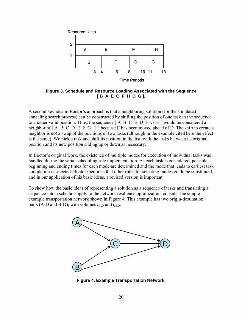
In a similar way, we can apply the scheduling rule to the sequence [ B A E C F H D G ] and obtain the schedule shown in Figure 3. The completion time for this schedule is 13, which is generally considered better than the 16 achieved for the first sequence, so we would prefer the second sequence to the first.
16104 6 9 143 7
1
2A C G
B D E F H
Resource Units
Time Periods
16104 6 9 143 7
1
2A C G
B D E F H
Resource Units
Time Periods
20
Figure 3. Schedule and Resource Loading Associated with the Sequence [ B A E C F H D G ].
A second key idea in Boctor’s approach is that a neighboring solution (for the simulated annealing search process) can be constructed by shifting the position of one task in the sequence to another valid position. Thus, the sequence [ A B C E D F G H ] would be considered a neighbor of [ A B C D E F G H ] because E has been moved ahead of D. The shift to create a neighbor is not a swap of the positions of two tasks (although in the example cited here the effect is the same). We pick a task and shift its position in the list, with the tasks between its original position and its new position sliding up or down as necessary. In Boctor’s original work, the existence of multiple modes for execution of individual tasks was handled during the serial scheduling rule implementation. As each task is considered, possible beginning and ending times for each mode are determined and the mode that leads to earliest task completion is selected. Boctor mentions that other rules for selecting modes could be substituted, and in our application of his basic ideas, a revised version is important. To show how the basic ideas of representing a solution as a sequence of tasks and translating a sequence into a schedule apply to the network resilience optimization, consider the simple example transportation network shown in Figure 4. This example has two origin-destination pairs (A-D and B-D), with volumes qAD and qBD.
Figure 4. Example Transportation Network.
11104 6 8 133
1
2A
C GB D
E F H
Resource Units
Time Periods
11104 6 8 133
1
2A
C GB D
E F H
Resource Units
Time Periods
A
B
C D
A
B
C D
21
Each of the five directional links has a delay function of the form:
iiii xbat
where xi is the volume on the link. Links are also assumed to have capacity limits, Ui, so that valid flows must have xi ≤ Ui for all links. Each origin-destination pair has two possible paths, and the O-D pairs interact via the link C-D. The flow pattern on the network is determined by an equilibrium condition (If both paths for a given O-D pair are used, the travel times for the two paths should be equal unless the flow on the shorter path is at capacity. No unused path may have a shorter travel time than a used path for the same O-D pair, unless the capacity of the shorter unused path is zero.). For purposes of this example, we will assume that qAD = 100, qBD = 200, and the link characteristics are as shown in Table 1. In the nominal (base) case, there is sufficient capacity on the links to carry the specified O-D traffic, but under some damage scenarios, there may be demand that cannot be met.
Table 1. Link Characteristics for Example Transportation Network.
Link Index From-To ai bi Ui 1 A-D 5 0.02 100 2 A-C 2 0.01 100 3 C-D 4 0.01 300 4 B-C 2 0.02 200 5 B-D 5 0.03 150
In the nominal case, the equilibrium flow pattern on the network is the set of link flows shown in Table 2, and there is no unmet demand. The total travel time for all users of the network is 2393 units. (Flows are shown rounded to the nearest whole unit, although the actual equilibrium calculations may involve fractional units.)
Table 2. Equilibrium flow for nominal (base) case.
As a specific damage scenario, assume that links 3-5 are severely damaged and out of service. This set of link losses means that there is no available path from B to D, and all the traffic on that O-D pair becomes unmet demand. The flow pattern on the network immediately following the damage event is summarized in Table 3. The total travel time is 700 units for the flow from A to D that can be accommodated.
To measure overall impact of the damage, assume that the “cost” of a unit of unmet demand is 20, so that the total travel cost in the damaged state is 700 + 20 (200) = 4700. The impact can be measured as the increase in total travel cost, relative to the nominal case, or 4700 2393 = 2307. Repair actions will focus on the three damaged links and can be undertaken in the three possible modes mentioned above (Normal, Emergency and Staged). Table 4 summarizes a set of characteristics for the repair actions in the various modes on the three links assumed for purposes of this example.
Table 4. Parameters for modes of repair on damaged links.
Link Mode Duration (periods)
Cost Capacity Increment
3 (C-D)
Normal 3 3000 300 Emergency 2 6000 300
Staged – Part 1 2 1800 150 Staged – Part 2 2 1800 150
4 (B-C)
Normal 5 4000 200 Emergency 3 8000 200
Staged – Part 1 3 2400 100 Staged – Part 2 3 2400 100
5 (B-D)
Normal 6 5000 150 Emergency 4 10000 150
Staged – Part 1 4 3000 75 Staged – Part 2 4 3000 75
To implement the idea of a sequence as defining a solution that implies a schedule, consider a general structure in which each link is listed with two stages, labeled (a) and (b). The precedence structure implies that stage (b) for a given link cannot be listed before stage (a) for the same link, but there are no precedence restrictions across links. Using the two-stage structure allows for situations where the Normal or Emergency modes are chosen for a particular link (in which case the (a) stage has duration and cost and the (b) stage becomes a dummy) or where the Staged mode is chosen (in which case both stages have duration and cost, but at the end of the first stage, partial capacity is restored). Thus, for the example problem, a possible valid sequence would be:
[ 3a, 5a, 3b, 4a, 4b, 5b ].
23
To evaluate this sequence as a possible solution, we must be able to choose modes for each link and construct a schedule of activities to determine the times at which capacity restoration occurs on individual links. The mode selection for tasks can be done as a “local random search” process. That is, we can sample modes for the link tasks randomly, generating a set of N trials for the same sequence. Each trial can be scheduled using a simple single-pass scheduling mechanism (like in the normal project scheduling process) and the trial that yields the earliest restoration of full capacity on all links can be chosen as the representative schedule for the current sequence. This selected schedule can then be evaluated using a series of network flow assignments. To illustrate this idea, consider the sequence listed above for the three links requiring repair and a small value of N (i.e., N = 5). The sample of mode choices for the three links is listed in Table 5.
Table 5. Sample of repair modes on damaged links for 5 trials.
Link Trial1 2 3 4 5
3 (C-D) Staged Normal Staged Normal Emergency4 (B-C) Normal Staged Staged Normal Normal 5 (B-D) Emergency Normal Normal Staged Emergency
For Trial 1, the set of mode selections implies the sequence really is as follows (because the 4b and 5b elements become dummies):
[ 3 (Staged – Part 1), 5 (Emergency), 3 (Staged – Part 2), 4 (Normal), -- , -- ]. For scheduling, we use the characteristics from Table 2-4, and assume that the resource limit is a limit on the total activity that can be sustained simultaneously. Two “units” of work can be undertaken simultaneously; an action in either Normal mode or Staged mode on a given link counts as one unit, and an action in Emergency mode counts as two units. For Trial 1, the simple serial scheduler proceeds as follows:
1) Part 1 of the staged effort on link 3 begins at time 0. 2) Emergency action on link 5 begins at time 2, when the stage 1 work on link 3 is finished
and resources are available. 3) Part 2 of the staged effort on link 3 begins at time 6, when link 5 is restored. 4) Normal action on link 4 begins at time 6, when link 5 is finished.
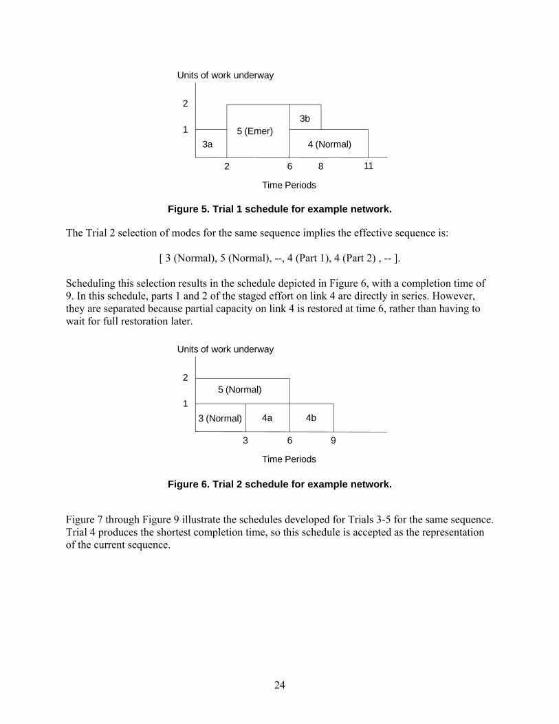
The illustration of this schedule is as shown in Figure 5. Complete restoration of the network capacity is at time 11.
24
Figure 5. Trial 1 schedule for example network. The Trial 2 selection of modes for the same sequence implies the effective sequence is:
[ 3 (Normal), 5 (Normal), --, 4 (Part 1), 4 (Part 2) , -- ]. Scheduling this selection results in the schedule depicted in Figure 6, with a completion time of 9. In this schedule, parts 1 and 2 of the staged effort on link 4 are directly in series. However, they are separated because partial capacity on link 4 is restored at time 6, rather than having to wait for full restoration later.
Figure 6. Trial 2 schedule for example network. Figure 7 through Figure 9 illustrate the schedules developed for Trials 3-5 for the same sequence. Trial 4 produces the shortest completion time, so this schedule is accepted as the representation of the current sequence.
1162 8
1
2
5 (Emer)
3a 4 (Normal)
3b
Units of work underway
Time Periods
63 9
1
25 (Normal)
3 (Normal) 4a 4b
Units of work underway
Time Periods
25
Figure 7. Trial 3 schedule for example network.
Figure 8. Trial 4 schedule for example network.
Figure 9. Trial 5 schedule for example network. For the schedule from Trial 4, there are changes in available link capacity at time 3 (restoration of link 3), time 4 (partial restoration of link 5), and time 8 (full restoration of both links 4 and 5). To evaluate SI for this schedule, we require two network flow assignments (for times 3 and 4). At time 8, the network returns to full service and the total travel time for that state (2393 units) is already known. At time 3, with link 3 restored to service, the resulting flow pattern is shown in Table 6. There is no available path from B to D, so there are still 200 units of unmet demand. The total travel time
1062 7
1
25 (Normal)
3a 4a3b
Units of work underway
Time Periods
4b
4
43 8
1
25a
3 (Normal) 4 (Normal)
5b
Units of work underway
Time Periods
62 11
1
2
5 (Emer)3 (Emer)4 (Normal)
Units of work underway
Time Periods
26
for the 100 units of flow from A to D is 650, so the total cost computed is 650 + 20 (200) = 4650. The impact measure for this state is 4650 2393 = 2257. Table 6. Equilibrium flow for partially restored condition at time 3 (unmet demand = 200).
At time 4, link 5 is partially restored to service (with capacity 75), and the resulting flow pattern is shown in Table 7. The unmet demand from B to D decreases to 125 units. The total travel time for the 175 units of flow accommodated on the network is 1194, so the total cost computed is 1194 + 20 (125) = 3694. The impact measure for this state is 3694 2393 = 1301. Table 7. Equilibrium flow for partially restored condition at time 4 (unmet demand = 125).
Computation of SI , i.e., the increase in travel cost relative to baseline conditions, for this solution is illustrated in Figure 10. SI is the area of the shaded region, or 14382 units.
Figure 10 . Measurement of SI for the example sequence. For this sequence, TRE is the sum of the costs incurred for the specific modes chosen in Trial 4: 3000 + 3000 + 3000 + 4000 = 13,000. If we use a weighting of = 1 to combine SI and TRE, our overall evaluation of this potential solution (sequence) is:
14382 (1)(13000) 27382J SI TRE
43 8
22572307
1301
Cost Impact
Time Periods
27
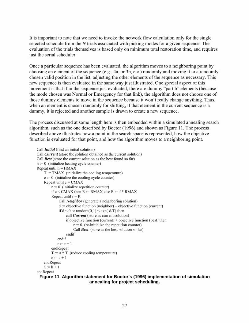
It is important to note that we need to invoke the network flow calculation only for the single selected schedule from the N trials associated with picking modes for a given sequence. The evaluation of the trials themselves is based only on minimum total restoration time, and requires just the serial scheduler. Once a particular sequence has been evaluated, the algorithm moves to a neighboring point by choosing an element of the sequence (e.g., 4a, or 3b, etc.) randomly and moving it to a randomly chosen valid position in the list, adjusting the other elements of the sequence as necessary. This new sequence is then evaluated in the same way just illustrated. One special aspect of this movement is that if in the sequence just evaluated, there are dummy “part b” elements (because the mode chosen was Normal or Emergency for that link), the algorithm does not choose one of those dummy elements to move in the sequence because it won’t really change anything. Thus, when an element is chosen randomly for shifting, if that element in the current sequence is a dummy, it is rejected and another sample is drawn to create a new sequence. The process discussed at some length here is then embedded within a simulated annealing search algorithm, such as the one described by Boctor (1996) and shown as Figure 11. The process described above illustrates how a point in the search space is represented, how the objective function is evaluated for that point, and how the algorithm moves to a neighboring point.
Call Initial (find an initial solution) Call Current (store the solution obtained as the current solution) Call Best (store the current solution as the best found so far) h := 0 (initialize heating cycle counter) Repeat until h = HMAX
T := TMAX (initialize the cooling temperature) c := 0 (initialize the cooling cycle counter) Repeat until c = CMAX r := 0 (initialize repetition counter) if c < CMAX then R := RMAX else R := f * RMAX Repeat until r = R Call Neighbor (generate a neighboring solution) d := objective function (neighbor) objective function (current) if d < 0 or random(0,1) < exp(-d/T) then call Current (store as current solution) if objective function (current) < objective function (best) then r := 0 (re-initialize the repetition counter) Call Best (store as the best solution so far) endif endif r := r + 1 endRepeat T := a * T (reduce cooling temperature) c := c + 1 endRepeat h := h + 1
endRepeat Figure 11. Algorithm statement for Boctor’s (1996) implementation of simulation
annealing for project scheduling.
28
29
3. APPLICATIONS AND ANALYSES
In this chapter we describe a set of case studies in which the bi-level programming model is developed and numerical optimization algorithms are applied. The first example includes a simple transportation network that minimizes transportation costs. This example provides a proof of concept on a relatively simple system in which we assume TRE is constant; hence, the optimal restoration sequence is the one that minimizes SI. In the second case study, the optimal resilience problem is formulated for a national rail system model. The R-NAS model is a static, nonlinear optimization model that predicts the flow of commodities across the national rail system on an average day. For this project, an interface was developed to simulate dynamic recovery of the system following a disruption. The project specifically investigated the optimal restoration sequence following a flooding event that disabled a set of bridges. The third application involves the development of a dynamic supply chain model for the munitions production. This example is rather different from the first two in that we do not attempt to identify an optimal restoration sequence. Rather, we investigated the ability to meet mission goals when production facilities were unable to receive input goods due to supplier outages or transportation disruptions. 3.1. Optimal Recovery Sequencing when TRE is Constant As a proof-of-concept demonstration, we investigate a simplification of the MRCPSP described by (15) – (20). 3.2.1. Problem Formulation Assume the flows across a network are governed by the minimum cost flow problem below (adapted from Bradley, et al. 1977): At a given time step, t,
j i
ijijtt cxzmin (21)
subject to: nibxx ij
kitj
ijt ,...,1 (22)
ijijtijt uyx 0 (23)
where
ijtx = the flow from node i to node j during time step t;
ijc = the unit transportation cost from node i to node j;
iju = the flow capacity from node i to node j;
0,1ijty denotes whether the link between node i and node j is functional at time t.
Equation (22) represents flow conservation, i.e., 0ib when node i is a source node, 0ib
when node i is a sink node, and 0ib when node i is a transshipment node.
30
For this investigation, we make the following simplifying assumptions and modifications to the MRCPSP described by (15) – (20):
1 0, , ,ijy i j D (24)
where D represents the set of disrupted network links.
0 1, ,ijy i j ; (25)
, 0.ijt ijmy y t m (26)
A single mode of recovery that returns a link to full capacity, 0iju , is available. The cost
of restoring capacity, i.e., restoration cost, is denoted by the variable ijr , and this cost is
constant with respect to time. Equation (24) describes the impact of the disruption on the network. In this scenario, capacities are reduced to 0, but sources and sinks are not affected. Equation (25) describes that all links are at full capacity prior to the disruption. Equation (26) indicates that after a link is repaired, it stays repaired. The impact of the final assumption is that TRE is constant in the optimal resilience problem (5). Hence, for this example, the mathematical formulation of the optimal resilience problem is as follows:
t
ty
zzSI 0min (27)
subject to
1
m
ijt ij m mt
y r R T
(28)
where tz and 0z are described by (21) – (23) and the variable mT represents the cumulative
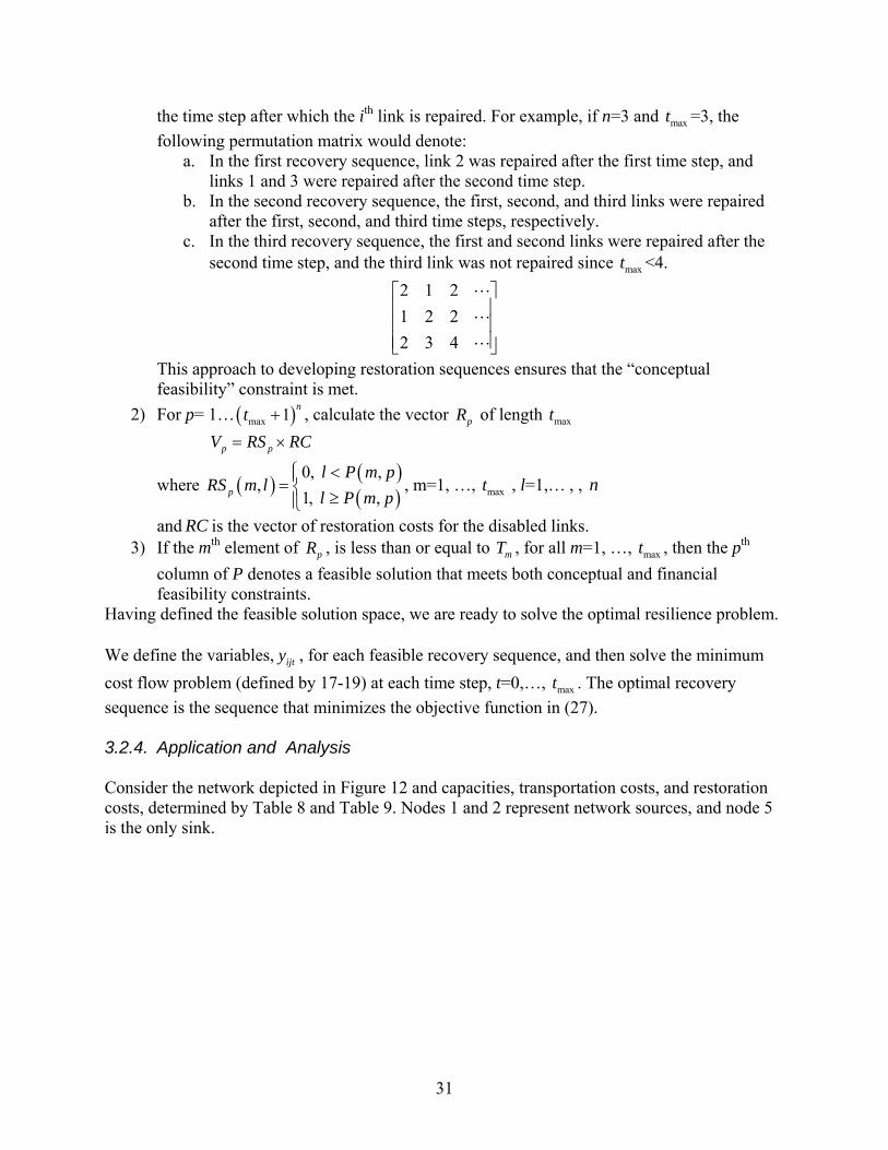
recovery resource constraints. In the bi-level optimization problem, (21) – (23) describe the inner loop problem and (27) and (28) describe the outer loop problem. Note that in this formulation, we assume uniform time steps where ∆ =1. The problem can be easily generalized for time steps of variable size. 3.2.3. Solution Methodology To solve the bi-level optimization problem, we adapt Kim, et al’s. (2008) solution approach. Inequalities (26) and (28) define the set of feasible solutions; that is, (26), termed the “conceptual feasibility” constraint by Kim, et al. (2008) indicates that once capacity is restored to a link, the capacity is maintained. The “financial feasibility” constraint, (28), indicates that the rate of recovery is limited by resource constraints. To define the feasible solution space, the following methodology was implemented:
1) Create the max 1n
n t permutation matrix, P, where each column consists of a
permutation (repetition permitted) of the integers 1, …, maxt . (The integer n denotes the
number of links to be repaired and maxt denotes the minimum number of time steps until
all links can be restored.) Each column in the matrix denotes a different restoration sequence, without regard to resource constraints, and the ith entry in a column indicates
31
the time step after which the ith link is repaired. For example, if n=3 and maxt =3, the
following permutation matrix would denote: a. In the first recovery sequence, link 2 was repaired after the first time step, and
links 1 and 3 were repaired after the second time step. b. In the second recovery sequence, the first, second, and third links were repaired
after the first, second, and third time steps, respectively. c. In the third recovery sequence, the first and second links were repaired after the
second time step, and the third link was not repaired since maxt <4.
2 1 2
1 2 2
2 3 4
This approach to developing restoration sequences ensures that the “conceptual feasibility” constraint is met.
2) For p= 1… max 1n
t , calculate the vector pR of length maxt
p pV RS RC
where
0, ,,
1, ,p
l P m pRS m l
l P m p
, m=1, …, maxt , l=1,… , , n
and RC is the vector of restoration costs for the disabled links. 3) If the mth element of pR , is less than or equal to mT , for all m=1, …, maxt , then the pth
column of P denotes a feasible solution that meets both conceptual and financial feasibility constraints.
Having defined the feasible solution space, we are ready to solve the optimal resilience problem. We define the variables, ijty , for each feasible recovery sequence, and then solve the minimum
cost flow problem (defined by 17-19) at each time step, t=0,…, maxt . The optimal recovery
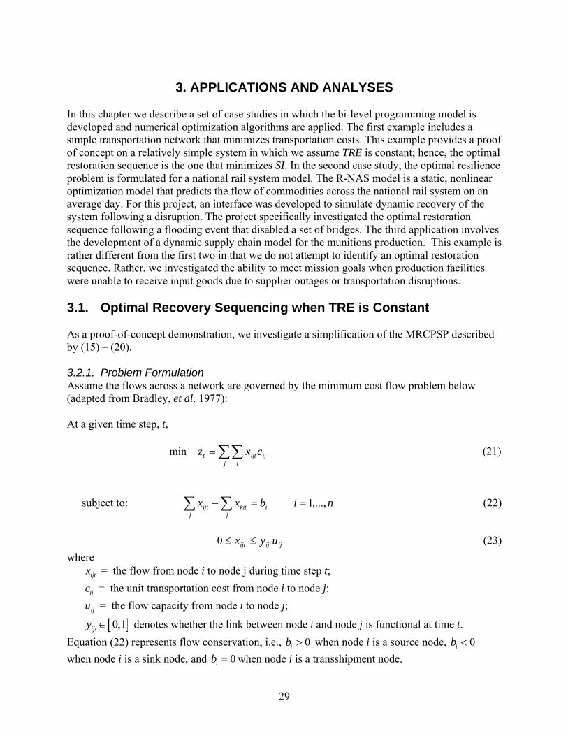
sequence is the sequence that minimizes the objective function in (27). 3.2.4. Application and Analysis Consider the network depicted in Figure 12 and capacities, transportation costs, and restoration costs, determined by Table 8 and Table 9. Nodes 1 and 2 represent network sources, and node 5 is the only sink.
32
(a)
(b)
Figure 12. Transportation Network (a) nominal state and (b) disrupted state. Red indicates links have no capacity.
In the nominal, undisrupted case, all flow (20 units) entering at node 1 goes to node 5 across link 1,5 and the 10 units of flow entering the network at node 2 go along link 2,4 and then 4,5 to node
1
3
5
4
2 1
3
5
4
2
33
5. Flow across link 1,5 is preferable since the transportation unit cost is cheapest across this link (5 per unit flow). The total transportation cost for the undisrupted case is 200 (20x5+10x5 + 10x5) (Table 10). When link 1,5 is disrupted and no capacity exists, flow from node 1 must be diverted along links 1,3 and 3,5. In this scenario, the optimal recovery strategy is to fix link 1,5 first, even though this takes 2 time periods for completion. Even though restoring capacity to link 1,4 reduces the transport unit cost from 10 to 9 for flow from node 1, those intermediate savings are not enough to offset the additional amount of time it takes to restore the preferred link, link 1,5 (Table 11).
Table 10. Optimal network flows when = 20.
Link i,j t=0 t=1 t=2 t=3 t=4
12tx 0 0 0 0 0
13tx 0 20 20 20 0
24tx 10 10 10 10 10
35tx 0 20 20 20 0
45tx 10 10 10 10 10
15tx 20 0 0 0 20
14tx 0 0 0 0 0
Transportation Costs
iz 200 300 300 200 200
SI=200
Table 11. Network flows when = 20 and link 1,4 is restored first. Link i,j t=0 t=1 t=2 t=3 t=4
12tx 0 0 0 0 0
13tx 0 20 0 0 0
24tx 10 10 10 10 10
35tx 0 20 0 0 0
45tx 10 10 30 30 10
15tx 20 0 0 0 20
14tx 0 0 20 20 0
Transportation Costs
iz 200 300 280 280 200
SI=260 If, however, the unit transportation costs across link 1,4, , is reduced from 4 to 2, and the nominal flow capacity across link 1,5 , is 10 instead of 20, the optimal restoration sequence changes (Table 12); link 1,4 should be restored before link 1,5. Immediately following the disruption, 10 additional units of flow from node 1 to node 5 are diverted from link 1,5 to links 1,3 and 3,5. This path has a unit transportation cost of 10. In this scenario, the optimal restoration
34
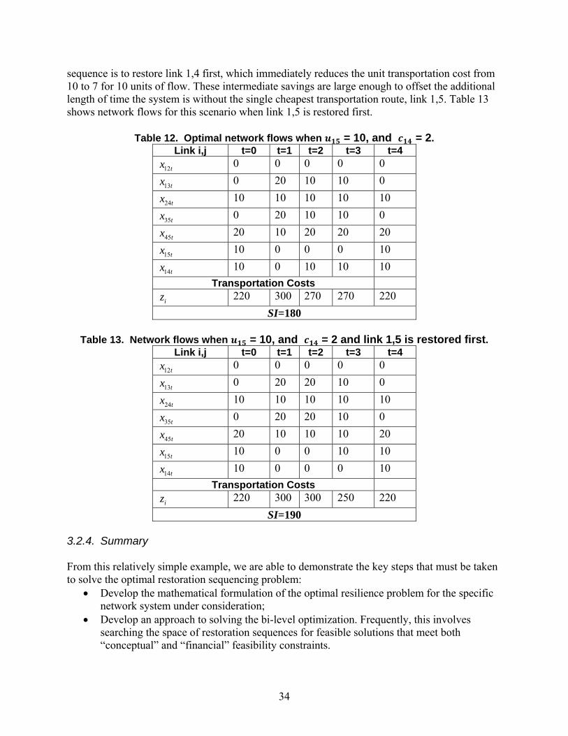
sequence is to restore link 1,4 first, which immediately reduces the unit transportation cost from 10 to 7 for 10 units of flow. These intermediate savings are large enough to offset the additional length of time the system is without the single cheapest transportation route, link 1,5. Table 13 shows network flows for this scenario when link 1,5 is restored first.
Table 12. Optimal network flows when = 10, and = 2. Link i,j t=0 t=1 t=2 t=3 t=4
12tx 0 0 0 0 0
13tx 0 20 10 10 0
24tx 10 10 10 10 10
35tx 0 20 10 10 0
45tx 20 10 20 20 20
15tx 10 0 0 0 10
14tx 10 0 10 10 10
Transportation Costs
iz 220 300 270 270 220
SI=180
Table 13. Network flows when = 10, and = 2 and link 1,5 is restored first. Link i,j t=0 t=1 t=2 t=3 t=4
12tx 0 0 0 0 0
13tx 0 20 20 10 0
24tx 10 10 10 10 10
35tx 0 20 20 10 0
45tx 20 10 10 10 20
15tx 10 0 0 10 10
14tx 10 0 0 0 10
Transportation Costs
iz 220 300 300 250 220
SI=190 3.2.4. Summary From this relatively simple example, we are able to demonstrate the key steps that must be taken to solve the optimal restoration sequencing problem:
Develop the mathematical formulation of the optimal resilience problem for the specific network system under consideration;
Develop an approach to solving the bi-level optimization. Frequently, this involves searching the space of restoration sequences for feasible solutions that meet both “conceptual” and “financial” feasibility constraints.
35
Implement solution methodology in software, when necessary. This step is likely necessary for models of “real” infrastructure systems.
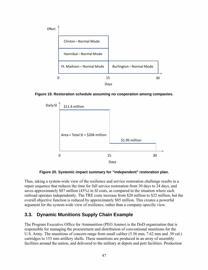
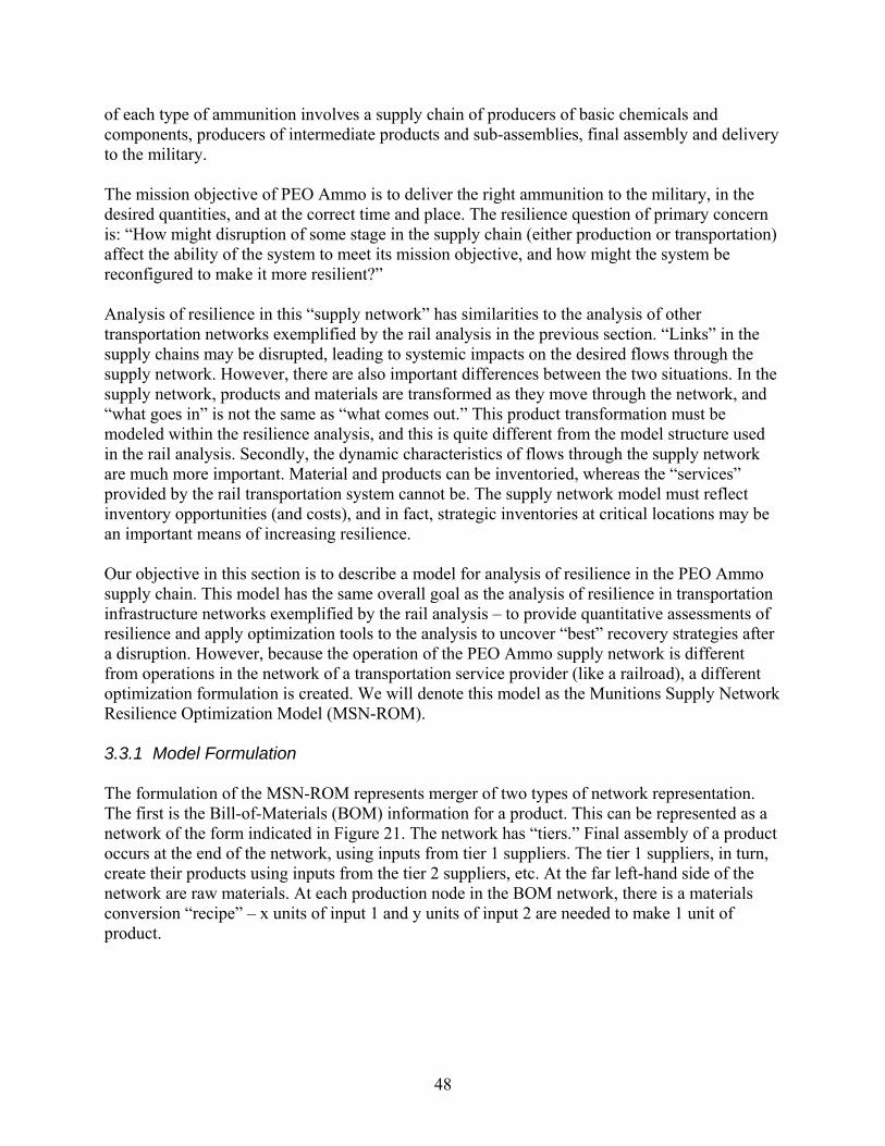
Analyze and validate results against other potential recovery sequences. In the following section, we apply this approach to a more complex model of the U.S. freight rail network. 3.2. Application to the U.S. Freight Rail Network The U.S. railroad industry originated about 26 million carloads of traffic in 2009, moving approximately 1.7 billion tons of commodities (Association of American Railroads, 2010). Industry freight revenue is approximately $46 billion annually. There are currently nine large railroads operating in the U.S., including seven U.S. companies (Class I railroads) and two Canadian companies. These nine large railroads are: Burlington Northern and Santa Fe Railway (BNSF), CSX Transportation, Canadian National (CN), Canadian Pacific, Grand Trunk Corporation, Kansas City Southern Railway, Norfolk Southern Combined Railroad Subsidiaries, Soo Line Railroad, and Union Pacific Railroad (UP). A wide variety of commodities move over the rail network, but in this case study we pay specific attention to five major categories: coal, grain, chemicals, motor vehicles and intermodal shipments. These five categories account for about 70% of total tonnage moved by rail. Coal is the primary single commodity moved by rail. Approximately 800 million tons of coal were moved by Class I railroads in 2009, accounting for 47% of all traffic (by weight). Much of this coal is used for electric power generation and support of other basic industries (such as steel). Many consumers of coal maintain substantial inventories, but an extended disruption in the ability of railroads to move coal could create a very significant economic impact. Railroads are major movers of grain from producing areas to food processing plants, as well as to ports for export. Grain makes up about 8% of total tons originated on Class I railroads, but in some areas (notably the Midwest) and during some parts of the year, grain movements are a much larger fraction of the total. Disruption in grain movements can affect domestic food supplies, national balance-of-payments accounts, and food supplies in many areas of the world. Chemicals make up about 10% of total tons moved on the rail network, and constitute about 14% of railroad revenue. These movements are important both because they are vital for many different industries and because many of the chemicals are considered hazardous materials. Railroads move approximately 70% of motor vehicles from assembly plants to distribution points. Motor vehicles constitute only about 1% of total tonnage moved, but because they are very high-value goods, revenue from moving motor vehicles is 5% of total revenue for Class I railroads. Intermodal shipments (i.e., the movement of containers or truck trailers on specialized rail equipment) account for approximately 6% of tonnage and 13% of total freight revenue for Class I rail carriers. There are about 10 million containers and trailers shipped via rail each year, and these movements tend to be concentrated in a few high-density corridors. Intermodal traffic tends to be high-value manufactured goods destined for final consumption, and disruption of these flows can have significant economic consequences.
36
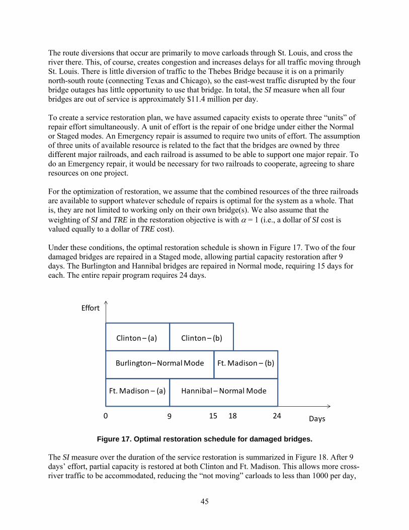
Our focus in this analysis is on the resilience of the rail network to a disruption that would cause outage of several major bridges across the Mississippi River between Iowa or Missouri (on the west side of the river) and Illinois (on the east side). Such an event might be the result of major flooding on the upper Mississippi River, for example. Chicago is the largest east-west interchange point in the rail network (where freight traffic is transferred between the western railroads and the eastern railroads), and the major rail lines going west from Chicago toward Kansas City, Omaha and Denver all cross the Mississippi River in this area. These major railroad bridges are “pinch points” for the rail network and crucial infrastructure elements to the national system. Specifically, the four bridges on which we focus are as follows.
1. Union Pacific Crossing at Clinton, IA
The Union Pacific main line west of Chicago crosses the Mississippi River at Clinton, IA. The very high traffic density on this line is illustrated in Figure 13. The crossing at Clinton is actually a series of three bridges. The main channel of the river is on the western (Iowa) side, and is spanned by a double-track steel truss bridge with a swing span that opens for barge traffic on the river. In the middle is the Illinois Channel Bridge, a double-track steel truss bridge with no moveable sections, and easternmost is the Sunfish Slough Bridge, a double-track steel plate girder bridge with no moveable sections.
Figure 13. Union Pacific traffic density (2007 data).
37
2. BNSF Bridge at Burlington, IA
West of BNSF’s major yard at Galesburg, IL, its main lines split, with one going west through Iowa and Nebraska to Denver, and the other going southwest to Kansas City. The line west to Denver crosses the Mississippi River at Burlington, IA. The bridge is a double-track steel truss bridge with a swing span to open for river traffic.
3. BNSF Bridge at Ft. Madison, IA
The BNSF main line between Chicago and Kansas City crosses the Mississippi River at Ft. Madison, IA. The bridge is a steel truss double-deck bridge that carries both auto and rail traffic (autos on the upper deck and rail on the lower). The bridge has a swing section to open for river traffic. The rail line is single-track, but carries very heavy traffic approximately 70 trains/day.
4. Norfolk Southern Bridge at Hannibal, MO
The Norfolk Southern line between Kansas City and Ft. Wayne, IN crosses the Mississippi River at Hannibal, MO. The bridge (sometimes called the Wabash Bridge) is a single-track steel truss bridge with a lift section for river traffic.
Our assessment of flow impacts from closure of these bridges focuses on a five-state area, including Nebraska, Kansas, Missouri, Iowa and Illinois, but within the context of a national rail network representation. The physical rail network that we are using is represented in Figure 14. This network does not include all rail track in the U.S. It focuses on the main lines that are used for long-distance movement and that carry high volumes of freight.
38
Figure 14. Representation of main lines in the national rail network. The impacts of outage of the four bridges will be felt most strongly within the five-state region that we have identified, and our focus in measuring systemic impact (SI) is on increases in car-miles and car-hours for diverted flows, and on movements that may not be made at all. In total, these three measures capture the direct economic impact of the disruption to normal flow patterns. The following subsections describe more details of this analysis – the national rail network flow model used to assess changes in flow patterns under various disruption and repair scenarios, the computation of overall SI and TRE for the restoration of normal service, the implementation of the optimization concepts from section 2 for this analysis, and the results of illustrative analyses. 3.2.1. The Rail Network Model The flows across specific links in the rail network depend on the volume of commodities to be moved between origins and destinations. In the real system, there are thousands of origin and destination points where individual shippers and receivers are located. However, for modeling purposes, we aggregate these points into a much smaller set of “zones” for origins and destinations of commodity traffic. Our set of zones, which we will refer to as Transportation Analysis Zones (TAZs), is illustrated in Figure 15. There are 84 TAZs defined, covering the lower 48 states of the continental U.S. We have not considered Alaska and Hawaii in the analysis because they are not directly affected by rail movements in the rest of the nation. Each TAZ is represented by a zone centroid – a major city within that zone that serves as the modeled origin
39
or destination for commodity movements for the entire zone. The volume of freight to be moved (within each commodity group) can then be summarized in an 84x84 table (referred to as an origin-destination, or O-D, table). These shipments (across all commodity groups) form the demand on the system.
Figure 15. Transportation Analysis Zones (TAZs) and centroids.
Given the set of commodity groupings of interest, the definition of TAZs and centroids, and the structure of the national rail network (including potential link capacity reductions or outages), the prediction of flows in the network is accomplished by a model called R-NAS (Rail Network Analysis System) developed at Sandia National Laboratories (Jones et al., 2003). The links in R-NAS have lengths (Li, in miles) and delay functions to represent travel time (in hours). The delay functions are of the generic form described in (14) in Section 2.1:
i
i
iiiiii K
xadKxd
1, 0 (29)
with iii Kxd , representing the time (in hours) for a carload to cross link i, when the flow
(measured in carloads/day) over the link is xi and the link capacity (also measured in carloads/day) is Ki . The value di0 represents the “free-flow” travel time across the link (i.e., without congestion, or when xi = 0). Different values of the parameters ai and i are used for
40
different classes of links in the network. R-NAS solves the optimization problem described in equations (15)-(20) in Section 2.1 to predict flows (by commodity group) over individual links in the represented rail network. When some link capacities are degraded (or zero), R-NAS predicts how flows will divert through the network to other links that are available. These diversions create additional costs (both distance and time-related), which are the basis for computing the SI measure. 3.2.2. Computing the SI and TRE Measures From the link flows (by commodity group) computed in R-NAS, total car-miles and total car-hours accumulated in the network can be computed. If (as a result of damage) the network becomes partially disconnected, some origin-destination pairs may not be serviced and carloads for those pairs will be recorded as not moved. These three basic measures (car-miles, car-hours and carloads not moved) can be converted into a (monetary) measure of SI as follows. In the base case (prior to any damage) the flows on the network result in a level of car-miles denoted M0 and a level of car-hours denoted H0. The carloads not moved are zero. In some damaged state at time t, the flows over the network produce car-miles Mt, car-hours Ht, and carload not moved Zt. The “extra” car-miles induced by the damage to the network, 0MMt ,
create additional costs. Average revenue per car-mile in the rail industry in 2009 was approximately $1.93 (Association of American Railroads, 2010). The operating ratio (ratio of total operating expenses to total operating revenue) for Class I railroads was 77.8% (Association of American Railroads, 2010), so an approximate estimate of the cost of an additional car-mile to the railroad is $1.50. This can be used to convert extra car-miles to dollars of SI. The costs of extra time in-transit include the costs of the in-transit inventory for the commodity being carried, the cost of extra car-time for the rolling stock, and the additional operating costs (more labor-hours, etc.). Most of the additional operating costs for train movements are captured by the change in car-miles, but the additional costs for yard operations are more time-related than distance-related. According to the 2007 Commodity Flow Survey, the average value of commodities moved by rail is $234 per ton (Bureau of Transportation Statistics, 2010). An average carload is 64.1 tons (Association of American Railroads, 2010), so the average value of a carload is approximately $15,000. Assuming a 10% cost of capital, the in-transit inventory carrying cost for an average carload is approximately $4 per day. Railway equipment can be either owned or leased, and leasing rates provide a mechanism for estimating average daily cost of the rolling stock. Leasing rates vary by car type, but are typically in the range of $400-$500 per car per month (Railway Age, 2008). On a daily basis, this can be expressed as $13-$17 per day, and we can use a value of $15 per car-day as an estimate. Additional operating costs (especially for yard delays) are difficult to estimate directly, but a reasonable estimate of the cost of delays is twice the cost of the in-transit inventory plus the car cost. This would imply a total estimate of $38 per car-day for excess delays. For shipments not moved, the cost to the shipper must be at least the cost of transporting the shipment. For railroads in 2009, the average revenue per carload was $1770 (Association of
41
American Railroads, 2010). We can use that as a rough estimate of the cost to the shipper of not moving the material. Thus, we can construct an estimate of SI as follows (where t is assumed to index days):
tttt ZHHMMSI 1770)(
24
38)(5.1 00 (30)
For each damaged link, we consider three modes of repair action:
4) “Normal”: Resources are applied to restore capability in an expeditious way. 5) “Emergency”: Additional resources are applied to accomplish the capacity restoration in
2/3 of the “Normal” time, but at a cost that is twice the “Normal” cost. 6) “Staged”: Capacity restoration is done in two stages. The first stage restores 50% of the
lost capacity in 60% of the time required for “Normal” restoration of full capacity, and at 60% of the “Normal” cost. A second stage of restoration can be done later to restore the remaining 50% of damaged capacity. The second stage of action also requires 60% of the “Normal” time, and requires 60% of the “Normal” cost.
Durations and costs for each mode are related to estimates for the Normal mode. We have used an estimate that the cost for Normal repairs to a damaged bridge is $5 million, and the duration is 15 days. Thus, an Emergency repair costs $10 million, but is completed in 10 days. A Staged repair restores 50% of capacity to the bridge in 9 days, at a cost of $3 million. The remaining 50% of capacity restoration requires an additional 9 days and an additional $3 million. In the analysis for the four Mississippi River bridges, these values are assumed to apply to each bridge, and create the Cim values noted in (7) of Section 2.1.
Thus, the overall objective function for the resilience optimization is:
Min
i m timtim
tttt yCZHHMMJ 1770)(
24
38)(5.1 00 (31)
The variables in this optimization (yimt) are binary, and are subject to constraints (14)-(17) noted in Section 2.1. Mt, Ht, and Zt are determined by R-NAS based on the solution to the nonlinear minimum-cost flow problem at time t ( (15)-(20) in section 2.1). 3.2.3. Implementation of the Simulated Annealing Algorithm with R-NAS The R-NAS RNR (Rail Network Resilience) software, hereafter referred to as RSW, is an implementation of Boctor’s (1996) simulated annealing (SA) algorithm that has been adapted for use with the R-NAS rail network model. As R-NAS itself is a static representation of the U.S. freight rail network and it represents flows across the network under a set of conditions for an average day, it was necessary to add the dynamics of network recovery to the model. Hence, the RSW targets a set of links (as specified by the configuration file) for disabling and then simulates how network flows change as links are repaired. Integration of this process with Boctor’s (1996) SA algorithm identifies the optimal restoration sequence and mode combination.
42
The following steps are performed in the RSW: 1. An XML configuration file is read in at initialization which defines all constant values
and target links (see the section “Configuration File” in Appendix A for a description of the structure and all parameters).
2. In order to establish a baseline for full capacity, the R-NAS network simulation is run and traffic flows are calculated with all links enabled (day = -1). The values for the length and baseline capacity are read from the R-NAS database and used for all future calculations. The flow calculations consist of the following:
a. Read the AB and BA flow values and times from the R-NAS link flow table (values change based on enabled/disabled links).
b. Calculate the car-hours for each commodity group (CG) via: (AB_time*AB_flow + BA_time*BA_flow)
c. Calculate the car-miles for each CG via: distance * (AB_flow + BA_flow) d. Aggregate the values calculated in (b) and (c) to get the total car-hours and car-
miles. e. Values for (b), (c) and (d) are stored for later use.
3. A second run of R-NAS is then performed with all target links disabled to determine the baseline constrained capacity (day = 0). Car-miles and car-hours are calculated and stored as in (2).
4. On day 1, repairs can be initiated and the software enters the “heating” cycle of the SA algorithm where the temperature is set to the maximum value.
5. The RSW then enters the “cooling” cycle where the temperature gradually decreases according to the SA parameters set in the configuration file.
6. Within the cooling cycle is a repetition loop where, for each iteration, the order of one link repair is randomly changed. Note that each link has 2 associated repairs to allow for a single repair (normal or emergency) or for a 2 stage repair with different start times. The order assignment has to ensure that for each link, the second repair always follows the first. In addition, if the current second repair is NULL (do nothing repair associated with a single repair mode), it will not be reassigned since the assumption is that it will not lead to a better ordering. This step in the process is searching the space of feasible restoration sequences.
7. Also within the repetition loop is an inner repair mode loop where multiple iterations are made to determine the optimal (shortest time) selection of repair modes across the target links for the current ordering. Part of this calculation depends on the resource threshold which limits the number of resource units that can be applied in parallel. Each type of repair has a defined resource usage depending on the link type being repaired and is in effect for the duration of the repair activity. The final repair order is used to generate a “change list” which delineates each day when a change in capacity occurs based on completed repairs.
8. For each day in the current “change list”, the RSW updates the capacity, duration and cost of repair for each target link and runs an R-NAS simulation. The car-miles/hours are calculated and stored as in (2) for each change day.
9. SI is calculated with Eq. 16 using the results from (2), (3) and (8) and aggregating the values in between change days. The formula is as follows:
43
a. SI = sum(over time)[sum(over CG) [REV_PMI*(CAR_MILES[t] - CAR_MILES[-1]) + REV_PHR*(CAR_HOURS[t]) - CAR_HOURS[-1])/24 + REV_CAR * CARLOADS_NOT_MOVED[t]]]
b. REV_PMI = Revenue per mile, converts car-miles into dollars (per CG, read from configuration file)
c. REV_PHR = Revenue per hour, converts car-hours into dollars (per CG, read from configuration file)
d. REV_CAR = Revenue per carload, the cost in dollars for not moving a carload (per CG, read from configuration file)
10. The TRE (Total Recovery Effort) is calculated as the sum of all repair costs determined in (8).
11. The objective function is calculated as: SI + α * TRE. The alpha value is read from the configuration file; typically, we use a value between 0 and 1.
12. The objective function for the test solution is compared to the current solution. If the value is smaller (better), then the algorithm sets the current solution to the test solution. If the value is larger (worse), determine if it should be set as current, dependent on the value of a random number (between 0 and 1) being less than exp(-diff/temp), where diff is ObjectiveFunc(test) – ObjectiveFunc(current) and temp is the current “temperature” in the SA algorithm. If the current solution is also better than the global optimum, set the global optimum equal to the current solution.
3.2.4. Results of the Analysis In addition to the four major bridges that are subject to damage in the experiments, the R-NAS network includes three other major Mississippi River bridges within the five-state region of interest, all south of the four that are subject to damage. There are two bridges in the St. Louis, Missouri, area (both operated by the Terminal Railroad Association of St. Louis), and the Union Pacific bridge near Thebes, Illinois, south of St. Louis. These locations are shown in Figure 16. In the event of inability to use some or all of the four bridges on which the analysis is focused, diversion of some rail traffic to these other three bridges is to be expected. However, such diversion would increase car-miles and car-hours, and hence be reflected in the systemic impact measure.
Figure 16. Locations of other Mississippi River crossings.
Thebes (UP)
St. Louis(2 bridges)
44
There are also three other rail bridges within the study area that may be usable in an emergency. The BNSF has bridges at Davenport, Iowa, and Quincy, Illinois, that are not normally very heavily used, but do provide some potential capacity. In addition, there is a Kansas City Southern bridge at Louisiana, Missouri. None of these bridges are on heavily used main rail lines, so they have not been included in the national network in R-NAS. The model thus does not predict diversion of traffic to these bridges and they are not considered further in this analysis. Under base case conditions (all seven bridges operating normally), a total of approximately 15,300 carloads cross the Mississippi River within the study area each day. Across the entire five-state area, the total daily car-miles and car-hours predicted by R-NAS (for each commodity group) are shown in Table 14.
Table 14. Summary of daily flow statistics within five-state region.
When all four bridges under analysis are out of service, there is substantial disruption to rail flows within the region, as summarized in Table 15. Most coal shipments are still made (i.e., the daily carloads not moved is quite small), but the total car-hours for the coal shipments nearly doubles, indicating very large delays. The total car-miles for grain shipments decreases because many shipments (about 700 carloads per day) are not being made at all. There is also a very large impact on intermodal shipments. Approximately 1100 carloads per day that would normally move through the region (along the major transport corridors) are not moved, and the movements that do occur suffer significant increases in distance and time as a result of route diversions. In total, some 5600 carloads per day do not move across the river.
Table 15. Summary of daily flow changes within five-state region with all four bridges out
The route diversions that occur are primarily to move carloads through St. Louis, and cross the river there. This, of course, creates congestion and increases delays for all traffic moving through St. Louis. There is little diversion of traffic to the Thebes Bridge because it is on a primarily north-south route (connecting Texas and Chicago), so the east-west traffic disrupted by the four bridge outages has little opportunity to use that bridge. In total, the SI measure when all four bridges are out of service is approximately $11.4 million per day. To create a service restoration plan, we have assumed capacity exists to operate three “units” of repair effort simultaneously. A unit of effort is the repair of one bridge under either the Normal or Staged modes. An Emergency repair is assumed to require two units of effort. The assumption of three units of available resource is related to the fact that the bridges are owned by three different major railroads, and each railroad is assumed to be able to support one major repair. To do an Emergency repair, it would be necessary for two railroads to cooperate, agreeing to share resources on one project. For the optimization of restoration, we assume that the combined resources of the three railroads are available to support whatever schedule of repairs is optimal for the system as a whole. That is, they are not limited to working only on their own bridge(s). We also assume that the weighting of SI and TRE in the restoration objective is with = 1 (i.e., a dollar of SI cost is valued equally to a dollar of TRE cost). Under these conditions, the optimal restoration schedule is shown in Figure 17. Two of the four damaged bridges are repaired in a Staged mode, allowing partial capacity restoration after 9 days. The Burlington and Hannibal bridges are repaired in Normal mode, requiring 15 days for each. The entire repair program requires 24 days.
Figure 17. Optimal restoration schedule for damaged bridges. The SI measure over the duration of the service restoration is summarized in Figure 18. After 9 days’ effort, partial capacity is restored at both Clinton and Ft. Madison. This allows more cross-river traffic to be accommodated, reducing the “not moving” carloads to less than 1000 per day,
0
Clinton – (a) Clinton – (b)
Hannibal – Normal Mode
9 24
Ft. Madison – (a)
Burlington–Normal Mode Ft. Madison – (b)
15 Days
Effort
18
46
and eliminating the most egregious delays at St. Louis. After day 9, the remaining “not moving” traffic is primarily some grain and “other” carloads. At day 15, full service is restored at Burlington, creating significant further improvements. The “not moving” carloads are eliminated, and the remaining delays are relatively minor. When all remaining service is restored at day 24, the daily system impact drops to zero.
Figure 18. Systemic impact summary for optimal restoration plan.
The total SI measure for this plan is approximately $117 million. The total cost of the repairs is $22 million, so the overall cost of this disruption is estimated at $139 million. One of the interesting comparisons for this overall resilience measure is to contrast it with a situation where the railroads operate independently, each repairing their own infrastructure. The restoration schedule for this situation is depicted in Figure 19, and the resulting SI summary is shown in Figure 20. Because the BNSF railroad has two bridges out, and can support one major repair at a time, they must be done in sequence. With this restoration sequence, the major change is at day 15, when service is restored on three of the four bridges. At that point, the number of cars not moving drops from about 5600 per day to approximately 1000 per day, and the additional costs (car-hours and car-miles) for traffic diversion drop substantially as well. The remaining SI costs over the final 15 days of the restoration effort are just under $2 million per day. In this mode of operation, it requires 30 days to restore full service to the network, and the total SI cost is approximately $204 million. However, since all bridges are repaired in Normal mode, the TRE costs are minimized, at $20 million.
0
$11.4 million
$2.1 million
9 24
Area = Total SI = $117 million $0.2 million
15 Days
Daily SI
18
47
Figure 19. Restoration schedule assuming no cooperation among companies.
Figure 20. Systemic impact summary for “independent” restoration plan.
Thus, taking a system-wide view of the resilience and service restoration challenge results in a repair sequence that reduces the time for full service restoration from 30 days to 24 days, and saves approximately $87 million (43%) in SI costs, as compared to the situation where each railroad operates independently. The TRE costs increase from $20 million to $22 million, but the overall objective function is reduced by approximately $85 million. This creates a powerful argument for the system-wide view of resilience, rather than a company-specific view. 3.3. Dynamic Munitions Supply Chain Example The Program Executive Office for Ammunition (PEO Ammo) is the DoD organization that is responsible for managing the procurement and distribution of conventional munitions for the U.S. Army. The munitions of concern range from small caliber (5.56 mm, 7.62 mm and .50 cal.) cartridges to 155 mm artillery shells. These munitions are produced in an array of assembly facilities around the nation, and delivered to the military at depots and port facilities. Production
0
Burlington – Normal Mode
Clinton –Normal Mode
30
Hannibal –Normal Mode
Ft. Madison – Normal Mode
15
Days
Effort
0
$11.4 million
Area = Total SI = $204 million
$1.95 million
15
Days
Daily SI
30
48
of each type of ammunition involves a supply chain of producers of basic chemicals and components, producers of intermediate products and sub-assemblies, final assembly and delivery to the military. The mission objective of PEO Ammo is to deliver the right ammunition to the military, in the desired quantities, and at the correct time and place. The resilience question of primary concern is: “How might disruption of some stage in the supply chain (either production or transportation) affect the ability of the system to meet its mission objective, and how might the system be reconfigured to make it more resilient?” Analysis of resilience in this “supply network” has similarities to the analysis of other transportation networks exemplified by the rail analysis in the previous section. “Links” in the supply chains may be disrupted, leading to systemic impacts on the desired flows through the supply network. However, there are also important differences between the two situations. In the supply network, products and materials are transformed as they move through the network, and “what goes in” is not the same as “what comes out.” This product transformation must be modeled within the resilience analysis, and this is quite different from the model structure used in the rail analysis. Secondly, the dynamic characteristics of flows through the supply network are much more important. Material and products can be inventoried, whereas the “services” provided by the rail transportation system cannot be. The supply network model must reflect inventory opportunities (and costs), and in fact, strategic inventories at critical locations may be an important means of increasing resilience. Our objective in this section is to describe a model for analysis of resilience in the PEO Ammo supply chain. This model has the same overall goal as the analysis of resilience in transportation infrastructure networks exemplified by the rail analysis – to provide quantitative assessments of resilience and apply optimization tools to the analysis to uncover “best” recovery strategies after a disruption. However, because the operation of the PEO Ammo supply network is different from operations in the network of a transportation service provider (like a railroad), a different optimization formulation is created. We will denote this model as the Munitions Supply Network Resilience Optimization Model (MSN-ROM). 3.3.1 Model Formulation The formulation of the MSN-ROM represents merger of two types of network representation. The first is the Bill-of-Materials (BOM) information for a product. This can be represented as a network of the form indicated in Figure 21. The network has “tiers.” Final assembly of a product occurs at the end of the network, using inputs from tier 1 suppliers. The tier 1 suppliers, in turn, create their products using inputs from the tier 2 suppliers, etc. At the far left-hand side of the network are raw materials. At each production node in the BOM network, there is a materials conversion “recipe” – x units of input 1 and y units of input 2 are needed to make 1 unit of product.
49
Figure 21. Bill-of-materials (BOM) network representation. The second type of network structure included in the formulation is the movements of materials across locations over time. This concept is illustrated in the network fragment shown in Figure 22. Different locations are represented as different “y-coordinates” in the network, and time advances along the “x-axis”. Two nodes at the same “height” in the network represent the same location at different times, and movement of material across an arc connecting them represents storage (inventory) of material at that location. An arc connecting two nodes at different “y-coordinates” and different “x-coordinates” represents transportation of material from one location to another, which requires some elapsed time. This “time-space” network structure is important for representing the dynamics of the supply network.
Figure 22. Time-space network representation of movements within a supply network. The MSN-ROM is formulated as a linear programming optimization, where the objective is to meet the mission delivery goals for final products, subject to possible limits on available materials, production capability and capacity at different locations, and transportation capacity between locations. Ideas contained in the model formulation have been drawn from several previous developments in capacity-constrained material requirements planning in manufacturing industries (e.g., Billington, et al., 1983; Maes, et al., 1991; Adenso-Diaz and Laguna, 1996. We consider a set of products indexed by i = 1, … I with the products in a subset being denoted as the final products. We denote time periods with index t = 1, … T. The MSN-ROM is formulated as follows:
Tier 2 suppliers
Tier 1 suppliers
Final Assembly
Tier 2 suppliers
Tier 1 suppliers
Final Assembly
Time
Locations
Time
Locations
50
i
T
tit
i
T
titit
i
T
t
mt VPmPe111
)(max (32)
such that
TtIiQSPQ itititti ,,1;...,,11, (33)
I
jitjtijititi TtiRPaSR
1)(,1, ,,1; (34)
TtIiRVR ititit ,,1;...,,1min (35)
TtIiUP itit ,,1;...,,1 (36)
TtIiKS itit ,,1;...,,1 (37)
T
tiit iDP
1
(38)
TtIiVSRQP ititititit ,,1;,10,,,, (39)
where: Pit = production of product i in period t
Qit = inventory of finished product i at the end of period t Rit = inventory of raw material i at the end of period t aij = units of product i required to produce one unit of a subsequent product j Vit = inventory shortage of raw material i at the end of period t Sit = units of product i shipped in period t Uit = production capacity for product i in period t Kit = shipment capacity for product i in period t
minitR = target minimum inventory for raw material i at the end of period t
Di = demand for final product i over the analysis horizon (i) = transportation delay for product i (from its origin to destination)
m = small positive value (e.g., .01) = relative weight on inventory targets The objective of the model in (32) contains a term that attempts to maximize output of all the final products, i , across all time periods. Because there is generally value in producing as much output as possible in early time periods (if there are available resources), the term e-mt
provides a small “discounting” of production in later time periods. The second term in the objective provides a small penalty cost on production of intermediate products, to prevent
51
solutions that produce excess amounts that are not used in subsequent products. The final term of the objective function represents a penalty on missing inventory targets for raw materials. Throughout the model, a distinction is drawn between “raw materials” and “products,” even though both are indexed by i, and both are within the set of all products. A good i is considered a product if it is still located where it was produced (i.e., from the perspective of that location it is a finished good). If it has been transported to a location where it will be used to make another product, it is (at that location) considered a raw material. Inventory targets are placed on raw materials, implying that those goods should have been transported to where they will be used, rather than held where they were produced. The first set of constraints (33) links production, shipments, and inventory of finished goods. At the beginning of period t, there is a finished-goods inventory of product i equal to Qi,t-1. During period t, Pit units of product i are processed, and Sit units are shipped out to their destination. The total of beginning inventory plus production, minus shipments, constitutes finished-goods inventory left at the end of period t. Constraints (34) link raw materials, arrivals of shipments from suppliers and production volumes. The raw materials in inventory at the end of period t-1 are augmented by arrivals of shipments from suppliers (after a delay in transit of (i) periods), and decreased by usage of the materials to create products. The aij coefficients represent the information in the bill-of-materials for each product. The remaining material constitutes raw material inventory at the end of period t. Constraint (35) measures the deviation from target values if the raw material inventory falls below min
itR . The deviation is Vit, and it is penalized in the objective function. If no strategic
inventory targets have been set (i.e., minitR = 0), these constraints have no effect on the solution.
Setting of inventory targets represents one way of increasing the resilience of the supply network, because it creates stocks of material that can be used to buffer disruptions affecting suppliers “upstream” of the inventory. Constraints (36) and (37) limit production and transportation activities, respectively. These constraints are used to reflect capacity constraints at production facilities, and also to allow specification of disruptions (e.g., a given production facility goes down for three periods, reflected by setting the capacity of that facility to zero for those periods). Constraints (38) limit the production of final products to the amounts required by the Army. With these constraints present, the objective function strives to meet, but not exceed, the specified delivery targets over the course of the planning horizon. 3.3.2 Illustrative Computations PEO Ammo maintains BOM information for the various types of munitions using a software tool called IBAT (Industrial Base Assessment Tool). Other required information for the MSN-ROM (facility locations, products and capacities, target inventory levels, etc.) can be obtained from planning staff at individual facilities in the supply network. However, the assembly of all this
52
information creates a fairly detailed picture of munitions production, which is sensitive. Thus, for purposes of this report, we have used some artificial data to illustrate the character of model solutions, without disclosing actual values. As an illustration, we consider three final products produced in two final assembly locations, a set of 42 parts/materials, and 22 supplier locations. Our analysis uses weekly periods, with a 13 week planning horizon and a single desired quantity of each final product to be delivered to the Army at the end of the 13 weeks. For this example, systemic impact (SI) is measured simply as the amount short in the delivery of each product at the end of the 13 weeks. In an initial experiment, we consider a three-week disruption at the beginning of the planning horizon in the final assembly location for product 1. The demand for product 1 is 2000 units to be delivered at the end of week 13, and the capacity of the assembly plant is specified to be 180 units/week. Quite clearly, with only 10 weeks to produce the product after the disruption (and no initial finished goods inventory in place), the delivery target cannot be met. Figure 23 shows this situation. The nominal production is 2000/13 154 units/week, so without the disruption, the target is achievable. However, when there is no production in the first three weeks, the plant cannot catch up, and ends the quarter 200 units short on this product.
Figure 23. Cumulative production of product 1 after three-week disruption at the
beginning of the planning horizon. As a second experiment, we consider a more complicated situation, where production of a tier 2 product (nitrocellulose) is disrupted for four weeks at the beginning of the planning horizon. The normal production limit on this product is 3000 units/week, but for the first four weeks, only 1000 units/week are produced. The downstream customer for this product is the tier 1 supplier who produces propellant used in both products 1 and 2. That supplier has a 3000 unit inventory of nitrocellulose on hand at the beginning of the analysis period. The initial raw material inventory helps sustain the propellant production and shipment to the final assembly plant, but it is insufficient to cover the whole shortfall in nitrocellulose production. Figure 24 shows the cumulative production of product 1, and Figure 25 shows the same data for product 2. Product 1 output is slowed over the first four weeks, but then sufficient propellant is allocated to allow its production to recover and meet the end-of-quarter target of 2000 units. However, this is at the expense of product 2. The end-of-quarter target for product 2 is 5000 units, but the constraint on
Product 1 Cumulative Production
0
500
1000
1500
2000
2500
0 2 4 6 8 10 12 14
Week
Un
its Nominal
Actual
53
the upstream production at the tier 2 supplier of nitrocellulose limits the production of propellant, which in turn “starves” the production of product 2 over the quarter, and the end result is a shortfall of approximately 1850 units.
Figure 24. Cumulative production of product 1 when production of a tier 2 material is
constrained.
Figure 25. Cumulative production of product 2 when production of a tier 2 material is
constrained. As a third experiment, we assume that the propellant manufacturer at tier 1 had a 6000 unit inventory of nitrocellulose at the beginning of the planning period, rather than a 3000 unit inventory. All other conditions are the same as in experiment 2. Figure 26 shows the cumulative production of final product 2 in this experiment. The larger initial inventory of raw material at the tier 1 supplier allows more propellant to be produced and this translates directly into a smaller impact on product 2 quantity. The shortfall in this case is approximately 1300 units. The larger initial inventory of raw material has not eliminated the entire problem, but it has improved
Product 1 Cumulative Production
0
500
1000
1500
2000
2500
0 2 4 6 8 10 12 14
Week
Un
its Nominal
Actual
Product 2 Cumulative Production
0
1000
2000
3000
4000
5000
6000
0 2 4 6 8 10 12 14
Week
Un
its Nominal
Actual
54
the resilience of the overall system and reduced the systemic impact of the disruption at the tier 2 supplier.
Figure 26. Cumulative production of product 2 when tier 1 supplier has larger initial raw
material inventory. 3.3.3 Extensions to the Model The MSN-ROM represented in equations (32)-(39) in section 3.3.1 contains an implicit assumption that each product is produced at one location. For several of the products in the munitions supply network, this is true, but it is not universally so. One of the next extensions of the model is to include multiple suppliers, with choices available at the next tier in the supply network. Having multiple potential suppliers for a given material/product is another way of increasing resilience in the supply network, and this extension will enhance the model significantly. A second extension is to include aggregate production constraints (across multiple products) at individual facilities. This will also make the model more flexible and realistic. The product-specific constraints currently present are effective for testing the effects of disruptions at a plant, but are not sufficient for reflecting overall capacity limits within the system. Third, we will add more detail about shipment of final products to military destinations (depots and ports), along with more detail about the desired shipment sizes and schedule. This will make the goals on production of final products more realistic.
Product 2 Cumulative Production
0
1000
2000
3000
4000
5000
6000
0 2 4 6 8 10 12 14
Week
Un
its Nominal
Actual
55
4. SUMMARY AND CONCLUSIONS The overall goal of this LDRD project was to advance the state of resilience science to enable the optimization of infrastructure recovery strategies in a constrained resource environment. Towards this effort, we have developed the theoretical, mathematical framework for identifying optimal recovery responses that minimize resilience costs. The optimal resilience problem that we have posed is a bi-level optimization problem. In the “inner” problem, we solve for network flows, and we use the “outer” problem to identify the optimal recovery modes and sequences. We have adapted solution techniques, previous leveraged for the Multi-Modal Resource Constrained Project Scheduling Problem, to numerically solve the optimization problem for a set of infrastructure models. We believe that this LDRD effort represents significant progress in the field of resilience science. The framework that we have developed is capable of including: the dynamics of recovery processes and feedback of these processes with system performance; accounting of resource expenditures from recovery processes; and identifying the optimal combination of recovery sequences and modes that minimize resilience costs in the context of constrained resources. These factors are unique within the set of quantitative resilience assessment capabilities currently being utilized for infrastructure assessment. Subsequent to developing the mathematical framework, we adapted a rail network model, R-NAS, that is currently being used for infrastructure analysis and applied the resilience framework to the model to develop an integrated resilience analysis and optimization capability. The integration of this framework with a complex, infrastructure model currently being used by NISAC, demonstrates the feasibility and benefit of this framework. To date, our research focus has been on how the system responds and evolves after a disruptive event. We believe that the next logical research and development area is the integration of system redesign with recovery responses to improve resiliency. One can think of this issue as a tri-level optimization problem. At the lowest level, there is an optimization to find flows in the network, given a current state of links/nodes. At the next level up, there is the optimization of sequencing/allocating recovery resources, necessary to quantify resiliency. If one adds the opportunity for system redesign, at a third level up, one has the optimization of reconfiguring/adding/redesigning pieces of the network to improve the achievable resiliency.
56
57
4. REFERENCES Adenso-Diaz, B. and M. Laguna (1996). "A Technique to Minimize Overtime in the Capacitated MRP Problem," Production and Operations Management, 5:4, pp. 357-370. Alcarez, J., C. Maroto and R. Ruiz, “Solving the Multimode Resource-Constrained Project Scheduling Problem with Genetic Algorithms,” Journal of Operational Research Society, 54, 2003, pp. 614-626. Association of American Railroads, Class I Railroad Statistics, May 24, 2010, available online at www.aar.org. Billington, P.J., J.O. McClain and L.J. Thomas (1983). "Mathematical Programming Approaches to Capacity-Constrained MRP Systems: Review, Formulation and Problem Reduction," Management Science, 29:10, pp. 1126-1141. Boctor, F.F., “Resource-Constrained Project Scheduling by Simulated Annealing,” International Journal of Production Research, 34:8, 1996, pp. 2335-2351. Bouleimen, K. and H. Lecocq, “A New Efficient Simulated Annealing Algorithm for the Resource-Constrained Project Scheduling Problem and Its Multiple Mode Version,” European Journal of Operational Research, 149, 2003, pp. 268-281. Bradley, S., A. Hax, and T. Magnanti, Applied Mathematical Programming, Addison-Wesley Publishing Company, Menlo Park, CA, 1977. Bruneau, M., S. Chang, R. Eguchi, G. Lee, T. O’ Rourke, A. Reinhorn, M. Shinozuka, K. Tierney, W. Wallace, and D. von Winterfeldt, “A Framework to Quantitatively Assess and Enhance the Seismic Resilience of Communities,” Earthquake Spectra 19(2003), pp. 737-38. Bureau of Transportation Statistics, Shipment Characteristics by Geography by Mode: 2007, U.S. Department of Transportation, Washington, DC, accessed online at http://www.bts.gov/publications/commodity_flow_survey/, 7/2/2010. Bush, G. W., “Homeland Security Presidential Directive-3 (HSPD-3),” Washington, D.C., 2002. Bush, G. W., “Homeland Security Presidential Directive-7 (HSPD-7),” Washington, D.C., 2003. Chang, S. and M. Shinozuka, “Measuring Improvements in the Disaster Resilience of Communities,” Earthquake Spectra, 20(2004), pp. 739-755.
58
Chen, W.-N., J. Zhang, H. S.-H. Chung, R.-Z. Huang and O. Liu, “Optimizing Discounted Cash Flows in Project Scheduling – An Ant Colony Optimization Approach,” IEEE Transactions on Systems, Man and Cybernetics, Part C, 40:1, 2010, pp. 64-77. Clinton, W., “Presidential Decision Directive PDD-63, Protecting America’s Critical Infrastructures,” Washington, D.C., 1998. Damak, N., B. Jarboui, P. Siarry and T. Loukil, “Differential Evolution for Solving Multi-Mode Resource-Constrained Project Scheduling Problems,” Computers & Operations Research, 36, 2009, pp. 2653-2659. Hartmann, S., “Project Scheduling with Multiple Modes: A Genetic Algorithm,” Annals of Operations Research, 102, 2001, pp. 111-135. Holling, C., “Resilience and Stability of Ecological Systems,” Annual Review of Ecology and Systematics 4 (1973), pp. 1-23 Jarboui, B., N. Damak, P. Siarry and A. Rebai, “A Combinatorial Particle Swarm Optimization for Solving Multi-Mode Resource-Constrained Project Scheduling Problems,” Applied Mathematics and Computation, 195, 2008, pp. 299-308. Jones, D.A., L.K. Nozick, M.A. Turnquist, M.W. Hollingsworth, C.R. Lawton, M.A. Ehlen, J.R. Davis, and D.W. Talso, Impact Analysis of Potential Disruptions to Major Railroad Bridges in the U.S. – Phase I Report, National Infrastructure Simulation and Analysis Center, Sandia National Laboratories, Albuquerque, NM, 2003. Jozefowska, J., M. Mika, R. Rozychi, G. Waligora and J. Weglarz, “Simulated Annealing for Multimode Resource-Constrained Project Scheduling,” Annals of Operations Research, 102, 2001, pp. 137-155. Kim, B. J., W. Kim, and B. H. Song, “Sequencing and Scheduling Highway Network Expansion Using a Discrete Network Design Model,” Ann. Reg. Science, 2008, 42, 621-642. Kolisch, R., and A. Drexl, “Local Search for Nonpreemptive Multimode Resource-Constrained Project Scheduling,” IIE Transactions, 43, 1996, pp. 987-999. Maes, J., J.O. McClain and L.N. Van Wasenhove. "Multilevel Capacitated Lot-Sizing Complexity and LP-Based Heuristics," European Journal of Operational Research, 53:2, pp. 131-148, 1991. Mori, M., and C.C. Tseng, “A Genetic Algorithm for Multimode Resource-Constrained Project Scheduling,” European Journal of Operational Research, 100, 1997, pp. 134-141. Ozdamar, L., “A Genetic Algorithm Approach to a General Category Project Scheduling Problem,” IEEE Transactions on Systems, Man and Cybernetics, Part C, 29:1, 1999, pp. 44-59.
59
Railway Age, “Railcar Market: What’s Equipment Worth Today?” June, 2008. Reagan, R., “Executive Order 13282, National Security Telecommunications Advisory Committee,” Washington, D.C., 1982. Rose, A. and S.-Y.Liao, “Modeling Regional Economic Resilience to Disasters: A Computable General Equilibrium Analysis of Water Service Disruptions,” Journal of Regional Science 45(2005), pp. 75-112. Sprecher, A., and A. Drexl, “Multimode Resource-Constrained Project Scheduling by a Simple, General and Powerful Sequencing Algorithm,” European Journal of Operational Research, 107, 1998, pp. 431-450. Transportation Safety Administration (TSA), “Transportation Systems Critical Infrastructure and Key Resources Sector-Specific Plan as input to the National Infrastructure Protection Plan,” Washington, D. C., 2007. Tseng, L.-Y., and S.-C. Chen, “Two-Phase Genetic Local Search Algorithm for the Multimode Resource-Constrained Project Scheduling Problem,” IEEE Transactions on Evolutionary Computation, 13:4, 2009, pp. 848-857. Vugrin, E. D., R. C. Camphouse, P. S. Downes, M. A. Ehlen, and D. E. Warren,“Measurement of System Resilience: Application to Chemical Supply Chains,” Proceedings of SIAM Conference on Mathematics for Industry: Challenges and Frontiers, San Francisco, October 9-10, 2009a. Vugrin, Eric D., R. Chris Camphouse, and Daniel Sunderland, Quantitative Resilience Analysis through Control Design, technical report SAND2009-5957, Sandia National Laboratories, September 2009b Vugrin, E. D., D. E. Warren, M. A. Ehlen, and R. C. Camphouse, “A Framework for Assessing the Resilience of Infrastructure and Economic Systems,” in Sustainable and Resilient Critical Infrastructure Systems: Simulation, Modeling, and Intelligent Engineering, Kasthurirangan Gopalakrishnan and Srinivas Peeta, eds., Springer-Verlag, Inc., 2010.
60
61
APPENDIX A: ADDITIONAL DETAILS FOR THE RAIL NETWORK RESILIENCE SOFTWARE
This appendix provides additional details on the testing and input-output details for the RSW. Evaluation of RNR Software In order to evaluate the efficacy of the SA algorithm, a comparison was made between running the SA algorithm versus a fully exhaustive search over all order and repair mode permutations for 5 rail links. In order to facilitate this comparison, a simplified network model (SNM) was developed to simulate each R-NAS run since a complete run of all iterations of the RSW using R-NAS requires over 70 hours. Using the SNM, a fully exhaustive search over all order/mode permutations took 449 minutes and found 27,556,200 solutions with an optimal solution value of 2,255,324 for the objective function. The SA algorithm using the SNM took 13.6 seconds and found 2796 solutions with an optimal solution value of 2,284,218 for the objective function (this was with 50 mode steps, 6 heating steps, 6 cooling steps, max repetition of 48 steps, and a repetition factor of 4). By comparison, the SA algorithm only required 0.05% the amount of time to generate a solution that was within 1.3% of the true optimal solution. The full R-NAS rail network is comprised of 5330 links of which 5064 are involved in the RSW link flow calculations. Additionally, there are 13 commodities which are tracked over the network. In order to determine the impact within a sub-network of the model (containing only the Midwest states of Iowa, Nebraska, Kansas and Missouri), only 946 links are examined. This area was chosen because it contains seven bridges that can be used to characterize the total flow within the region. Of these seven bridges, four were selected as the target links for disabling/repairing during the simulation and are captured in the configuration file. Input Files The RSW uses the following two files for configuration of an analysis run:
Configuration File (rnrSchema.xml) – Provides the various RNR (Rail Network Resilience) constants related to link types, repair types, commodity groups and overall optimization. Also contains a list of the target links to be disabled and repaired (see the section on the configuration file for more details).
Selection Set (MidwestLinks.txt) – Provides a listing of all links of interest in a single column text file. If this file is not specified in the configuration file, all links in the R-NAS database are used for the analysis.
Output Files The RSW produces the following two files at completion:
CommoditySums.csv – A comma-separated values file which holds the final optimal solution of the SA process as a single table of flow values. The column is the flow value (Total Carloads, Carloads Not Moved, Carloads Moved, Car-Hours, Car-Miles) for each commodity group and the row is the day on which these values were calculated. In addition, the values of the objective function, SI, TRE and all pertinent optimization
62
constants are included along with a listing of the optimal Link Repair order. Each link entry is formatted as follows: <link ID> [<repair mode> <start day(s)>]. Note that staged repairs have 2 start days separated by a colon specified in the link repair list (e.g., 1234 [staged 1:4]).
ComSumDaily.csv – A comma-separated values file which holds the flow values broken out by day and commodity group as well as the list of constrained links per day with capacity following each link ID. This file holds all iterations of the SA algorithm, but not the sub-iterations where the minimum time for each repair sequence is determined.
Object Model of RSW The RSW is an object oriented package written in the C# language (version 2.0) using Microsoft Developer’s Studio 2005. The following is a list of all classes used by the RSW with descriptions of their responsibilities as well as their dependencies. The source code is stored in the TeamForge project https://teamforge-web.sandia.gov/sf/projects/r_nas_resilience. Class Name: RNASTest Description: This class is the main driver application which is also used to interface to the TransCAD application for executing R-NAS runs. Responsibilities:
Initializes all connections to TransCAD in order to interact with the R-NAS model Provides the main SA algorithm for generating all solution.
Dependencies: Utilizes the RepairMgr class for parsing the configuration file and computing/storing
solutions to each candidate repair strategy. Calls the R-NAS model for every day that a repair is completed within the repair strategy
Class Name: RepairMgr Description: The Repair Manager class holds all possible repair modes and link repair information. It is used to drive most optimization calculations and stores the associated solution. Responsibilities:
Parses the input configuration file. Calculates, stores and saves all intermediate and final solutions. Provides the algorithms for iterating across all repair modes and orderings, either
randomly or sequentially. Dependencies:
Utilizes the C# XML parser for parsing the configuration file. Uses the RepairMode class for storing the characteristics associated with executing a
specific repair mode on a link. Uses the RepairLink class for storing the characteristics associated with repairing a
specific link type. Uses the Link class for holding the target links which are to be disabled and then
repaired. Uses the Repair class for determining a repair strategy ordering.
63
Uses the StateCounter class for sequentially iterating across all repair ordering and/or mode permutations.
Uses the ConstantGroup class to store all constants related to the optimization process. Uses the CommodityGroup class to store the constants associated with each commodity
group. Class Name: RnrNode Description: The RNR (Rail Network Resilience) Node class holds a collection of RNR properties associated with a particular node (i.e., Commodity Group, Link, Repair Link, or Repair Mode). It provides a mapping from each node in the XML configuration file to the appropriate software object. This is the base class for many of the other classes used within the RSW. Responsibilities:
Provides the ability to parse each XML node and convert all XML attributes to key-value pairs (referred to as “properties”).
Provides an interface for retrieving properties as string, integer or double values. Provides basic validation capability for ensuring that certain properties appear within the
RnrNode. Dependencies:
Utilizes the C# XML parser for parsing configuration file XML tags.
Class Name: RepairLink Description: The Repair Link class holds the repair characteristics pertinent to repairing a particular type of link (normal, yard, bridge). Responsibilities:
Provides method for parsing a link repair node from the XML configuration file. Dependencies:
This class is derived from the RnRNode class. Utilizes the C# XML parser for parsing configuration file XML tags.
Class Name: RepairMode Description: The Repair Mode class holds the repair characteristics pertinent to the mode used for repairing a link (mode, duration, cost, resource utilization, restored capacity, and probably of choosing this repair mode). Responsibilities:
Provides method for parsing and validating a link repair mode from the XML configuration file.
Dependencies: This class is derived from the RnRNode class.
Class Name: ConstantGroup Description: The Constant Group class holds all of the global constants related to performing the RNR optimization. Responsibilities:
Provides method for parsing and validating a collection of constant value nodes from the XML configuration file.
64
Provides methods for efficiently retrieving the constant values as integer or decimal values.
Validates all constants according to their type (integer, decimal or string). Dependencies:
This class is derived from the RnRNode class. Utilizes the C# XML parser for parsing configuration file XML tags.
Class Name: CommodityGroup Description: The Commodity Group class holds all of the RNR constants associated with a particular Commodity Group (e.g., Coal). Responsibilities:
Validates that all required properties are specified for each commodity group (revenue per carload, cost per mile, cost per hour).
Dependencies: This class is derived from the ConstantGroup class.
Class Name: Link Description: The Link class represents a physical link in a rail network: normal, bridge or yard. One of these entities can have zero (NULL repair mode), one (NORMAL or EMERGENCY repair modes) or two (STAGED repair mode) Repairs. The Repair period is inclusive such that if start = 3 and end = 5, then the link is being repaired on days 3, 4 and 5. Responsibilities:
Provides an interface for retrieving the properties associated with a rail link. Provides an interface for updating the repair modes and duration(s) associated with
repairing the link. Dependencies:
This class is derived from the RnRNode class.
Class Name: Repair Description: The Repair class represents a repair action to be performed on a rail link. It encapsulates the start time, repair method (normal, emergency, stage1 stage2), duration, cost, and resources required. The duration and cost are modified according to the link type (normal, yard, bridge) for which the repair is targeted. Responsibilities:
Provides an interface for initializing the properties associated with a link (duration, cost, restored capacity).
Dependencies: None Class Name: StateCounter Description: The StateCounter class is used to iterate a collection of objects through a sequence of states. The objects can all have the same number of states or they can each have unique values. Responsibilities:
Provides methods for sequentially iterating a collection of objects through a sequence of states.
Provides a method for generate all unique permutations of a sequence.
65
Dependencies: None Class Name: StrUtil Description: The String Utility class provides string parsing functionality beyond what is provided by the standard C# String class. Responsibilities:
Provides methods for converting from strings to numbers (integer, decimal) and vice-versa.
Provides parsing methods for converting numeric string sequences into collections of numbers (integer, decimal).
Provides parsing methods for converting delimited string sequences into collections of string objects.
Dependencies: None Configuration File The configuration file for the RSW is in XML format and is broken into the following sections:
constant group – This section is a collection of numeric (integer or decimal) and/or string constants utilized by the software. Each constant is represented by an empty tag where the tag name is the constant name, the “type” attribute is the type (“int”, “dec” or “str”), and the “value” attribute is the constant value. The following constants are delineated in the file:
o diff_norm – The difference normalization factor which is used to normalize the difference between the objective function values for the candidate solution and the current solution. This factor is required such that when the candidate solution is worse than the current solution, the exponential of the negative difference is a finite value between 0 and 1. Values too large will drive the exponential to zero which the normalization factor is used to guard against. (Simulation value = 1e6.)
o number_mode_steps – The number of steps to iterate when choosing an optimal repair mode for the current repair sequence. This value equates to the number of permutations to examine when selecting an optimal repair combination for all affected links and will likely be less than the total number of permutations. (Simulation value = 50.)
o resource_threshold – The maximum number of resource “units” that can be applied in parallel. This value correlates with the “resource” attribute specified in the repair mode.
o weight_TRE – The “alpha” multiplicative factor applied to the TRE (Total Recovery Effort) before being added to the SI (System Impact) to compute the final objective function: SI + α * TRE
o max_heat_steps – The number of steps to iterate during the “heating” cycle of the SA (Simulated Annealing) algorithm.
o max_cool_steps – The number of steps to iterate during the “cooling” cycle of the SA algorithm.
o max_repetition – The number of steps to iterate within each step of the cooling cycle.
66
o repetition_factor – The multiplicative factor to apply to the max_repetition value on the last step of the cooling cycle.
o max_temperature – The maximum temperature to be set prior to each cooling cycle.
o cooling_factor – The multiplicative factor to be applied to the current temperature in each step of the cooling cycle.
o sim_carloads_not_moved – The maximum value of carloads not moved when using the simplified network model (i.e., when not using TransCAD).
o sequential_repair_order – A true/false (1/0) value indicating if the repair order should be selected randomly for each iteration or if all permutations should be iterated across in sequential order.
o sequential_repair_mode – A true/false (1/0) value indicating if the repair mode should be selected randomly for each iteration or if all permutations should be iterated across in sequential order.
o single_repair_mode – A true/false (1/0) value indicating if only a single repair mode should be specified and evaluated. In order for this option to work properly, the “repair_mode” and “start” attributes must be specified in each target link (described below) in order to define the single repair mode.
o use_transcad – A true/false (1/0) value indicating if the TransCAD software should be used for the network simulation or if the simplified network model should be applied.
o selection_set – The name of the file which specifies the subset of links to use when calculating all flow values for a sub-network. The file is a columnar text listing of all links to include in the analysis. If this tag is not included, then all links within the R-NAS database are included in the analysis.
o total_flow_set – The collection of links which define the total flow over a sub-network defined by a selection set. The type is “string” and the value is a comma-separated list of link IDs which are used to calculate the total flow. The baseline case (day = -1), defines the total carloads moved. The carloads not moved statistic is calculated by finding the flow across these links (when one or more are disabled) and subtracting from the baseline value.
repair info – This section describes the different types of links that can appear in the model as well as the types of repairs that can be performed (normal, emergency, stage1, stage2). It contains the following tags:
o link – The type of link that can appear in the model (normal, bridge or yard) which is described by the following tags: duration – The duration required for the repair of a link of this type. The
duration can be of type “fixed” where the value is a fixed number of days or “per_mile” where the value is the number of days per mile required to fix the link in addition to a “base” number of days.
cost – The cost associated with repairing a link of this type. The cost can either be “fixed” where the value is the exact number of dollars required or “per_mile” where the value is the dollars per mile for such a repair.
o mode – The repair mode to be performed which is described by the following attributes: type – the repair type name (normal, emergency, stage1 or stage2)
67
duration – the multiplicative time factor (e.g., “1” indicates that the repair takes as long as the duration indicated by the link type whereas ”0.66” indicates that the repair takes only 0.66 times the duration indicated by the link type).
cost – multiplicative cost factor (e.g., “1” indicates that the repair cost is equal to the value defined by the link type whereas ”2” indicates that the repair costs twice as much as indicated by the link type).
resource – the number of resource “units” required to perform the repair over the specified duration (e.g., twice as many resources are required to perform an emergency repair as compared to a normal repair).
capacity – the multiplicative capacity of the link after the repair is complete (e.g., “1” indicates the link has full capacity whereas “0.5” indicates that the link has 50% capacity).
prob – the probability that this type of repair is selected (e.g., “0.4” indicates a 40% probability that this repair type is selected).
target links – This section delineates which links should be included in the analysis to be disabled and repaired. Each link is described by its type (as described above) and an ID which is the link ID used within the R-NAS model environment. In order to test out a specific repair scenario, two additional attributes can be added to each link:
o repair_mode – Indicates the repair mode to be applied to the link (normal, emergency or staged).
o start – Indicates the start day on which the repair is to be performed. If the repair mode is “staged”, then this value will contain the start day of stage 1 followed by the start day of stage 2 with a colon separator (e.g., “1:4”).
commodity group info – This section enumerates all commodities and their associated constants. The following constant values are defined:
o revenue_per_mile – converts car-miles into dollars o revenue_per_hour – converts car-hours into dollars o revenue_per_carload – converts carloads not moved into dollars o capacity – used in simulation (non R-NAS mode) to determine the fraction of
flow attributed to each CG. The sum of this value across all CGs must equal 1.
The following is an example of an RNR configuration file: <?xml version="1.0" encoding="UTF-8" standalone="yes"?> <RNR> <constant_group id="global"> <diff_norm type="dec" value="1e6"/> <number_mode_steps type="int" value="50"/> <resource_threshold type="int" value="3"/> <weight_TRE type="dec" value="1"/> <max_heat_steps type="int" value="6"/> <max_cool_steps type="int" value="6"/> <max_repetition type="int" value="48"/> <repetition_factor type="dec" value="4"/> <max_temperature type="dec" value="8"/> <cooling_factor type="dec" value="0.25"/> <sim_carloads_not_moved type="int" value="650"/> <sequential_repair_order type="int" value="0"/>
DISTRIBUTION 1 MS 0484 Bob Hwang 8004 1 MS 0757 J. R. Russell 6484 1 MS1138 Ray Trechter 6381 1 MS1138 Lillian Snyder 6371 1 MS1161 D. Rondeau 5430 1 MS1315 John Brewer 10542 1 MS0899 Technical Library 9536 (electronic copy) 1 MS0123 D. Chavez, LDRD Office 1011