The published version of the paper can be found at http://www.inderscience.com/jhome.php?jcode=ijsse and should be cited as: Eric D. Vugrin, Mark A. Turnquist, Nathanael J. K. Brown. (2014). “Optimal Recovery Sequencing For Enhanced Resilience And Service Restoration In Transportation Networks,” Int J of Critical Infrastructures, 10(3/4), p.218-246.

Sandia National Laboratories is a multi‐program laboratory managed and operated by Sandia Corporation, a wholly owned subsidiary of Lockheed Martin Corporation, for the U.S. Department of Energy’s National Nuclear Security 

Administration under Contract DE‐AC04‐94AL85000. SAND 2013‐4852J 

OPTIMAL RECOVERY SEQUENCING FOR ENHANCED RESILIENCE AND SERVICE RESTORATION IN

TRANSPORTATION NETWORKS

ABSTRACT

Critical infrastructure resilience has become a national priority for the U.S. Department of Homeland Security. Rapid and efficient restoration of service in damaged transportation networks is a key area of focus. The intent of this paper is to formulate a bi-level optimization model for network recovery and to demonstrate a solution approach for that optimization model. The lower-level problem involves solving for network flows, while the upper-level problem identifies the optimal recovery modes and sequences, using tools from the literature on multi-mode project scheduling problems. Application and advantages of this method are demonstrated through two examples.

Key words: infrastructure resilience, optimization, transportation networks, project scheduling

1 INTRODUCTION AND BACKGROUND  Until recently, critical infrastructure protection (CIP) focused on physical protection and asset hardening (e.g., Reagan 1982; Clinton 1998; Bush 2002, 2003). However, a recent shift includes resilience ̶ the ability to prepare for and adapt to changing conditions and withstand and recover rapidly from disruptions (Obama 2013). The transportation infrastructure sector was one of the first sectors to incorporate resilience into its sector-specific plan when the Transportation Security Administration (TSA) made “Enhance the resilience of the transportation system” one of its top three priorities (TSA 2007).

This paper provides an approach for considering the role of recovery decisions in network resilience. Recovery is certainly not the only factor that determines resilience, but it is an important element of strategies to increase resilience. The approach described herein uses a project-oriented perspective to recover from the effects of a network disruption: that is, a set of repair tasks must be scheduled in an optimal way. Each of those tasks requires resources and time. Despite the obvious connections to the substantial literature on project scheduling, a primary difference of recovery work is that completion of a subset of tasks has value because partial operation of the network may be restored. In contrast, project scheduling generally focuses on minimization of makespan, which is time to completion of the entire project. This difference in focus leads to important differences in how schedules are evaluated.

Another difference between standard project scheduling and recovery scheduling is that optimization of recovery task scheduling evaluates the state of the system at a given time, requiring computation of network flows. Frequently, the flows are the result of a different optimization by network users. Thus, objective function evaluations require solution of another optimization. This bi-level optimization structure connects the work described here to prior work on optimization models for network design, in particular dynamic models in which the state of the system evolves over time. This work builds on crucial ideas from that literature, but the structure of time periods, tasks, etc. in the current context is considerably different from the multi-period network design models.

Section 2 of the paper discusses the general issues of measuring system resilience and describes recent related work. A specific mechanism for measurement of system resilience in the current context is also proposed. Section 3 provides the description of the model and a solution methodology, and Section 4 illustrates how it performs in some small-scale test cases. Section 5 draws conclusions and discusses implications for further research.

2 

2 RESILIENCE, SYSTEM IMPACT, AND RECOVERY FROM DISRUPTIONS 

Holling (1973) provided the first systems-level definition of resilience. Over the past four decades, many alternative definitions were proposed for infrastructure and economic systems analysis (e.g., see Fiksel 2003; Rose and Liao 2005; Tierney and Bruneau 2007; Park et al. 2013; Obama 2013). All these definitions include aspects of a system withstanding disturbances, adapting to the disruption, and recovering from the state of reduced performance.

Much recent research has been conducted to ascertain systemic features and attributes that characterize resilience. Bruneau et al. (2003) assert that resilience consists of “4 Rs”: robustness, redundancy, resourcefulness, and rapidity. They further assert that resilience encompasses four dimensions: technical, organizational, social, and economic. Madni (2009) proposes a set of qualitative design methods (heuristics) for resilience, including redundancy, reorganization, adaptation, and other features. Park et al. (2013) assert eight resilient design strategies including diversity, adaptability, cohesion, and other features. Katina and Hester (2013) focus system defensive properties such as deterrence, detection, delay, and response to characterize resilience of critical infrastructure systems. Resilience attribute analysis is still an active area of research as no consensus has been reached on fundamental system attributes that determine resilience.

Various metrics have been proposed for resilience measurement. Attribute-focused metrics typically consist of indices that rely on subjective assessments (e.g., Sempier et al. 2010; Fisher and Norman 2010) or data-based indicators (e.g., Cutter et al. 2010) that quantify system attributes that are asserted to contribute to resilience. Alternatively, performance-based methods (e.g., Bruneau et al. 2003; Chang and Shinozuka 2004; Rose 2007) propose metrics that measure the consequences of infrastructure disruptions and the impact that system attributes have on mitigating those consequences. Instead of quantifying system attributes to assess the indirect impact they have on an infrastructure’s ability to deliver critical goods and/or services, performance-based metrics directly measure outputs of the infrastructure system during the recovery period. . Most resilience metrics for transportation networks are categorized as performance-based methods as they focus on impacts to flows across the network during recovery activities.

While many system features can contribute to resilience, system recovery and its role in infrastructure network resilience has attracted much previous attention. Important examples across a range of infrastructure types include Xu et al.’s (2007) work on electric power restoration, Clausen et al.’s (2010) work on airline system recovery, Luna et al.’s (2011) work on water distribution networks, and Wang et al.’s (2011) work for internet protocol (IP) networks. These efforts represent a variety of approaches and criteria, as well as a range of different network types.

The recent work by Bocchini and Frangopol (2012), Chen and Miller-Hooks (2012), and Henry and Ramirez-Marquez (2012) provided three different perspectives on resilience and recovery in transportation networks. All three approaches draw upon a common concept underlying many resilience analysis approaches, as illustrated generically in Figure 1.

3 

Figure 1: Generic concept of disruption and recovery. Note that the length of the recovery period and 

impact on performance depends upon the disruption and network context. 

Some system performance measure, F, has a nominal value (i.e., under normal operating conditions) F0. The system operates at this level until suffering a disruption at time t0. The disruption generally causes a deterioration in system performance to some level Fmin at time t1. Recovery commences, affecting and likely improving network performance. Frequently, multiple options exist for sequencing recovery activities, and network performance is ultimately a function of recovery decisions (Figure 2). These decisions can include sequencing of repairs, selection of different repair modes that can hasten or slow restoration of network components, and resource allocation that can enable simultaneous repair of multiple links. Ultimately, system performance achieves a targeted level of performance (often taken to be F0) at a later time t2, and recovery is then considered complete.

Figure 2: Recovery variation under different recovery strategies 

Henry and Ramirez-Marquez (2012) are primarily interested in constructing and evaluating different metrics for system resilience. They view resilience as the ratio of recovery to loss (at a given time, t), and

form a measure min

0 min

( )( )

F t FR t

F F

. This formulation is identical to Rose’s (2007) static resilience

metric when Fmin is taken to be Rose’s worst-case quantity. Henry and Ramirez-Marquez (2012) apply this metric to a series of disruption scenarios that disable links in a transportation network in order to find restoration sequences that maximize recovery at a given time. To do so, the team makes three simplifying assumptions:

1. Link repairs are assumed to be discrete tasks.

Time, t

Nominal

Actual Performance

F(t)

F0 = F(t0)

Fmin = F(t1)

t0 t1 t2

Time, t

Nominal

Recovery with actions a1 at cost c1

F(t)

F0 = F(t0)

Fmin = F(t1)

t0 t1 t2

Recovery with actions a2 at cost c2

4 

2. Only a single link can be repaired at any given time. Hence, the optimization is purely a sequencing issue. Resource allocation for recovery activities is not a decision variable in the optimization.

3. A single recovery mode is assumed for network repairs. Consequently, the time for repair for a single link is constant and not affected by decision variables in the optimization.

Bocchini and Frangopol (2012) present a model of recovery planning for networks of highway bridges damaged in an earthquake. The model identifies bridge restoration activities that maximize resilience, minimize the time required to return the network to a targeted functionality level, and minimize the cost of restoration activities. The authors measure resilience with the following equation:

2

1

22 1

( )t

t

F t dt

Qt t

where F, t1, and t2 are as defined in Figure 1 above.1 This formulation resembles Bruneau et al.’s (2003) resilience loss calculation with one significant difference. Rather than measuring the area between F0 and F(t), Bocchini and Frangopol (2012) measure the area between F(t)and 0 and then normalize over the recovery time period. The advantage of this approach is that an increase in Q2 implies an increase in resilience; Bruneau et al.’s formulation has the opposite result.

Bocchini and Frangopol (2012) formulate a bi-level optimization structure, in which flows on the network are determined by a traffic assignment computation (solution to a lower-level optimization), and decisions on a recovery strategy are identified in an upper-level optimization. Bocchini and Frangopol model bridge capacity restoration as a continuous process associated with a rate of expenditure of funds. Decision variables for each bridge are the time to begin repairs and the rate of expenditure on that facility and are modeled as continuous variables. As funds are expended on a bridge, capacity is returned proportionately and partial capacity is available to the traffic flow computation. Although constraints are placed upon funding rates at individual facilities, the only constraint on the overall rate of expenditure is the sum of the maxima for each bridge. Total funds available over the planning horizon are constrained, but there is no limitation on the number of restoration efforts that can be active simultaneously. The result in their case study (involving a network of 38 bridges) is that most of the bridges have repairs starting immediately after the disruption (28 of 38 in one sample solution, and 32 of 38 in another). In light of likely limits on availability of required equipment and other resources, this may be unrealistic. Chen and Miller-Hooks (2012) focus on intermodal freight transportation networks and formulate a problem of finding a strategy for maximizing the proportion of original demand that can be accommodated at a given time after a disruption, subject to an overall budget constraint for restoration activities. Restoration is achieved by completion of a set of discrete recovery activities. Completion of those recovery activities results in a discrete change in link capacity, but each activity is represented as a single task. Each task has a cost and duration, but the only resource constraint is a limit on total recovery budget. Chen and Miller-Hooks (2012) assume explicitly that recovery of all damaged network links begins simultaneously immediately after the disruption. Their optimization model is aimed at selecting the set of recovery activities (which may include multiple options for each damaged link, with different effects on

1 Bocchini and Frangopol (2012) assume t0 = t1, i.e., the degradation is effectively instantaneous. This assumption is

reasonable given the short period of time required for earthquake damage to be realized when compared to recovery periods.

5 

restored capacity), so that the total amount of demand met within a given time is maximized. Timing of recovery activities and operational costs are not considered.

From the description of these three approaches, a number of key technical differences can be seen. These differences are important not only because they affect the problem formulation but also because they impact numerical solution of the optimization. The following section introduces a new, more general model for evaluating how recovery action decisions affect the restoration and resilience optimization in transportation networks. As previously noted, network recovery is one of many aspects that affects the resilience of transportation networks. However, the following discussion focuses on how previous research on transportation network recovery can be generalized under this framework.

3 A NEW RESILIENCE MODEL FOR TRANSPORTATION NETWORKS 

3.1 GENERAL FORMULATION 

Vugrin et al. (2010) developed a resilience framework that simultaneously considers restoration of system performance and the resource expenditures required to do so. Under this framework, the two key quantities calculated are systemic impact (SI) – the cumulative impact of decreased system performance following a disruption – and total recovery effort (TRE) – the cumulative resources expended in recovery activities. As illustrated in Figure 2, recovery decisions and actions affect both of these quantities.

Vugrin et al. integrate these quantities in a composite resilience measure:2

Z SI TRE (1)

where is a weighting factor that serves for both unit conversion and relative weighting between SI and TRE in overall evaluation. In any particular application, SI itself may be composed of several different measures of system performance (with relative weights), and those weights together with the factor serve to normalize Z to some useful scale. The framework was applied to continuous, dynamic systems (Vugrin and Camphouse 2011) and agent-based models (Vugrin et al. 2010). The following section describes calculation of SI and TRE when the framework is applied to transportation networks.

3.2 CALCULATION OF SYSTEMIC IMPACT AND TOTAL RECOVERY EFFORT FOR TRANSPORTATION NETWORKS 

The application context of interest here is transportation networks composed of discrete nodes and links. Disruptions create damage to nodes and/or links in the network. Damage is modeled as a reduction in the capacity of the links.3 Capacity reductions cause some flows across the network to be diverted to other facilities or perhaps to be blocked entirely. Flow diversions may increase congestion in other parts of the network and generally increase costs. In some cases not all flows can be accommodated, which creates additional systemic impact.

In this analysis, consider the network to contain a set of links indexed by i. At time t, the capacity of link i

is Ki(t). Under normal operations, the collection of link capacities is denoted as 0iK . At time t = 0, a

2 Vugrin et al. (2010) divide Z by a normalization constant, but that factor is omitted in this discussion because this

simplification is equivalent for optimization. 3 If node capacities are important in a specific application problem, they can be converted to equivalent link

capacities by introducing additional links and nodes into the network.

6 

disruption reduces some of the link capacities, and the initial post-event state is defined by a set of link

capacities, Ki(0), where for damaged links Ki(0) < 0iK .

Traffic on the network moves from origin nodes to destination nodes, and the volume in period t for origin-destination pair rs is denoted qrs(t). In a disrupted state, the network may have insufficient capacity to carry all the origin-destination traffic, and the volume of travel from r to s that cannot be accommodated at time t is denoted ers(t). Movement of origin-destination flows across the network induces a set of link flows, xi(t), and some total cost for link i, denoted as Hi[xi(t)]. This cost may reflect travel time, distance, fuel consumption, or other factors. In the nominal (non-disrupted) state, the network

flows are 0 ( )ix t and the total cost on link i is 0 0( ) ( )i i iH t H x t .

This analysis is based on a set of discrete time periods, indexed by t = 1,…,T, where T is the length of the planning horizon. The systemic impact is then defined as the increase in total cost, including both increases in total costs for flows on links and penalty costs ( rs ) for demand that cannot be

accommodated.

0

1

( ) ( ) ( )T

i i i rs rst i rs

SI H x t H t e t

(2)

The use of cost as a performance measure for SI means that the degraded performance implies an increase, rather than a decrease in the performance measure as illustrated in Figure 1, and the computation of the area between the nominal and degraded performance is above the nominal line rather than below it, but this does not alter the basic concept.

Measurement of TRE is related to the scheduling of repair tasks on damaged links in the network. These repair tasks have duration, require specific resources, and may be scheduled to begin in specific time periods during the planning horizon. At the completion of specified milestones in the repair effort, a specified increment of capacity is returned to function on link i. Repair to restore capacity on a damaged link may be represented as a single overall task, or as a project network with a collection of related tasks and milestones.

Repair tasks require resources of one or more types; in general, tasks may be scheduled in one of a set of possible modes. Repair task j on link i, scheduled in mode m and initiated in period t, is assumed to imply:

A lag duration of ijm periods before the task is completed;

Resource requirement kijmr for resource k in each period that the task is active; and

An associated total cost ijmC (which may be a net present value if discounting is necessary in a

given situation).

The set of modes available may not be uniform across all tasks and the set of tasks required for different links may also vary, but to avoid notation that is excessively cumbersome, use the ijm subscripting to imply using mode m selected from the set available for task j and a task relevant to recovery on link i.

The central variables in the recovery optimization model are:

1

0ijmt

if task j on link i is initiated in mode m in period tu

otherwise

Then

ijm ijmti j m t

TRE C u (3)

7 

Taken together, eqs. 1-3 define the objective, Z, to be minimized in the model designed to find an optimal recovery plan. This objective includes both the impact (SI) and recovery effort (TRE) elements of resilience and reflects the perspective of recovery planning as a challenge of scheduling repair tasks to restore damaged capacity in the transportation network. The following section defines the full model in detail.

3.3 OPTIMIZATION MODEL FORMULATION 

To make the model statement as compact as possible, eqs. 1-3 are combined into the objective in eq. 4.

0

1

( ) ( ) ( )T

i i i rs rs ijm ijmtt i rs i j m

Min Z H x t H t e t C u

(4)

The decision variables in this minimization, ijmtu , are subject to several constraints. They also must be

connected explicitly to the network flows, xi(t), the cost functions, Hi, and the unmet demand, ers(t). The authors discuss first the constraints on the ijmtu variables, and then their connections to the other model

elements.

Task j for link i can be performed in only one selected mode and will not be scheduled more than once. In some cases, it may not be scheduled at all, so

1 ,ijmtm t

u i j (5)

Tasks j and l for link i may have precedence constraints (e.g., j must be completed before l can begin). These constraints are written as follows:

ilmt ijm ijmtt m t m

t u t u (6)

In some cases, a mode for a task may allow it to be interrupted (i.e., complete part of it, stop, and complete the remainder later). In cases where the repair to a link is considered one aggregate task, completion of the first part may restore partial capacity. In this case, the aggregate task can be broken into two sub-tasks with a precedence constraint and a milestone is associated with completion of the first task.

In general, link repairs require some physical resources in limited supply, and availability of these resources may constrain recovery scheduling. These resource constraints are applied in the form:

1

,ijm

tk

ijm ijm kti j m t

r u R k t

(7)

where Rkt is the available amount of resource k in period t.

Other constraints on repair task scheduling may be appropriate in specific applications, but eqs. 5-7 represent the general types of constraints that are likely to be most common.

The scheduling of repair tasks affects flows and impacts in the network through the provision of link capacity. As a result of completion of specified tasks j (i.e., achievement of milestones) for link i, the

capacity of link i in period t is augmented by ij . The available capacity on link i in period t is written as:

8 

1

( ) (0)ij mt

i i ij ij mj

K t K u

(8)

The link capacities generally are important for determining flow patterns in the network, which ultimately affect eq. 1.

3.4 NUMERICAL SOLUTION 

The upper problem in the recovery optimization resembles a multimode project scheduling problem. The multimode resource-constrained project scheduling problem (MRCPSP) is a challenging optimization problem that received considerable attention from a variety of researchers. Finding exact solutions to the MRCPSP is computationally intense, but several types of heuristics proved capable of finding good (but not necessarily optimal) solutions and are scalable to realistic problem instances. Mori and Tseng (1997), Ozdamar (1999), Hartmann (2001), and Alcaraz et al. (2003) proposed various forms of genetic algorithms. Kolisch and Drexl (1996) explored ideas of local neighborhood search for finding good solutions, and Tseng and Chan (2009) combined genetic algorithm ideas with local search to create a two-phase algorithm. Other recent work by Jarboui et al. (2008) and Chen et al. (2010) explored using particle swarm and ant colony optimization approaches, and Damak et al. (2009) tried a differential evolution approach. Algorithms for the MRCPSP are generally based on a criterion of minimizing the time to project completion (often called makespan). This criterion is important because evaluation of the objective function is trivial, in that the algorithm simply tallies the completion time of the final task. Consequently, the algorithms can afford to evaluate the objective function a large number of times without incurring much computational penalty. For the recovery model described in Section 3.3 above, evaluation of the objective function for the upper-level problem involves solution of several lower-level optimization problems to construct network flows at different times. Evaluation of this objective function is much more computationally expensive; thus, a solution method that recognizes this challenge must be constructed. Simulated annealing is a useful class of meta-heuristics applied to the MRCPSP (e.g., Boctor 1996, Bouleimen and Lecocq 1997, and Jozefowska et al. 2001). Boctor’s approach is particularly well-suited for the recovery optimization problem. A core idea of Boctor’s approach to the project scheduling problem is that a potential solution can be described as an ordered list, or sequence, of tasks. The sequence implies a schedule, which can be constructed relatively easily. In the multimode case, the sequence also contains mode selection for each task (which implies its duration and resource requirements). Sequences can also be checked easily for validity (i.e., no task can appear in the sequence before any of its required predecessors or after any of its successors). A second key idea in Boctor’s approach is that a neighboring solution (for the simulated annealing search process) can be constructed by shifting the position of one task in the sequence to another valid position. In Boctor’s original work, the existence of multiple modes for execution of individual tasks was handled during the serial scheduling rule implementation. As each task is considered, possible beginning and ending times for each mode are determined; the mode that leads to earliest task completion is selected. Boctor mentions that other rules for selecting modes could be substituted. The authors developed two key modifications that improve the efficiency of the search method significantly. The first is that the solution process can memorize the SI values for specific capacity conditions. Different recovery sequences produce the capacity changes at different times, but timing differences of these capacity changes does not necessarily affect travel times, unmet demand, and other factors that contribute to SI values. By identifying the changes that affect capacity , it is possible to calculate SI quantities for those changes and to store those values. Using this approach, the optimization routine can call the stored

9 

value rather than re-evaluating the objective function. This process can reduce computational requirements substantially in both simple and complex networks. Bocchini and Frangopol (2012) recognized this general concept in their solution algorithm. They observed in later stages of their search process that approximately two-thirds of the required solutions are simply retrieved from previously stored results and do not need to be recomputed. A second important computational element for the simulated annealing process is that because capacity changes on links occur at discrete times, it is quite easy to characterize solutions that are dominated. That is, if the order of link capacity restorations is the same in potential solution a as it is in potential solution b, but in solution a none of the changes occur later than in b, and at least one change occurs earlier, solution a will dominate solution b in the calculation of SI. In this case, if the SI for solution a was already computed, calculations for solution b are unnecessary. The algorithm can discard solution b and proceed to another candidate solution. The addition of the memorization and dominance features are effective at reducing the computational burden of the optimization process, as will be shown in later sections.

3.5 COMPARISON TO OTHER METHODOLOGIES 

The modeling assumptions, problem formulation, and solution method described above differ significantly from the previous efforts of Henry and Ramirez-Marquez (2012), Bocchini and Frangopol (2012), and Chen and Miller-Hooks (2012). Henry and Ramirez-Marquez (2012) discuss the idea of allocating resources to enable network recovery in an optimal way, but limit their consideration to situations in which links are repaired strictly in sequence (one link at a time). Their concern is with a sequence that maximizes the degree of recovery at a given time. Their approach is one special case of the optimization problem formulated in 3.3.

The Bocchini and Frangopol (2012) analysis has several common elements with the optimization problem formulated here, as well as some important differences. They use a similar bi-level structure, in which flows on the network in any particular state are determined by a traffic assignment computation (solution to a lower-level optimization), and decisions on a recovery strategy are in an upper-level optimization. They also consider similar measures of systemic impact and recovery cost. A major difference is the characterization of recovery actions. This leads to a very different formulation of the upper-level problem.

Bocchini and Frangopol (2012) model capacity restoration as a continuous process associated with a rate of expenditure of funds, rather than treating restoration as a sequence of discrete tasks. They include a global constraint on fund availability across the entire planning horizon, but they do not consider time-dependent resource availability. Consequently, there is no limit on the number of tasks that can be conducted simultaneously.

Chen and Miller-Hooks (2012) consider a set of discrete recovery activities and completion of those recovery activities results in a discrete change in link capacity. However, each activity is represented as a single task. Each task (recovery option) has a cost and duration, but no other requirements for constrained resources. Similar to the Bocchini and Frangopol approach, the only resource constraint is a limit on total recovery budget.

4 ILLUSTRATIVE EXAMPLES 

This section considers two different network examples to illustrate application of this new resilience formulation. The first example, drawn from Henry and Ramirez-Marquez (2012), includes a simple maximum flow network. This example demonstrates that the Henry and Ramirez-Marquez approach is a special case of the formulation presented in this paper. The second (more complicated) example considers a congested traffic flow network.

10 

4.1 EXAMPLE 1: A MAXIMUM FLOW NETWORK 

4.1.1 PROBLEM FORMULATION 

Consider the network shown in Figure 3 with link capacities in Table 1. Assume the objective is to maximize flow from node 1 to 7. Link flows are determined by solving a maximum flow problem, given the state of the link capacities. The link flow costs (Hi[xi(t)] in eq. 4 of the optimization problem in Section 3.3 are irrelevant and are assumed to be zero. Optimization occurs through the usual method of introducing a return link, 7-1, with unlimited capacity, and maximizing the flow 71x , subject to the link capacities and flow conservation at all nodes. The

flow problem at time t can be written as:

max 71( )x t (9)

s.t. ( ) ( ) 0 1,...,7n n

i ii I i O

x t x t n

(10)

0 ( ) ( )i ix t K t i (11)

The sets In and On in eq. 10 are the inbound and outbound links at node n, respectively. In the nominal (undisrupted) case, the maximum flow is 14 units. The SI measure is the reduction in flow, 17 71( ) 14 ( )e t x t , for the single origin-destination pair of interest.

Figure 3: Maximum flow network for Example 1 

Table 1: Network capacities for Example 1 

Link  Capacity  Link  Capacity 

1‐2  5  3‐5  4 

1‐3  7  3‐6  5 

1‐4  4  4‐6  4 

2‐3  1  5‐7  9 

2‐5  3  6‐5  1 

3‐4  2  6‐7  6 

1

2

3 7

4

5

6

5

3

7

4

4

5

4

1

9

6

1

2

11 

A disruption scenario defined by Henry and Ramirez-Marquez (2012) is used for analysis:

1. The event (at time 0) reduces the capacity of links 1-2, 1-3, 1-4, 2-3, and 3-4 to 0.

2. A single-mode repair action mode is available for each damaged link. Table 2 lists durations and costs for these actions.

3. Resource constraints prevent repair of multiple links simultaneously.

4. Full capacity for a link is restored only after completion of the repair. Restoration of partial link capacity does not occur.

Table 2: Repair characteristics for Example 1 

Damaged Link 

Repair Duration: �i  (periods) 

Repair Cost: Ci 

1‐2  20  20,000 

1‐3  50  50,000 

1‐4  40  40,000 

2‐3  20  20,000 

3‐4  10  10,000 

Because there is only one mode for each of the repair tasks and the link repairs are specified as a single task for each link, the task scheduling variables for the links that have been damaged (denoted as set L) can be simplified to uit, and each task i L has a cost Ci and a duration i. For

i L , define (0) 0iK and 0i iK , for i L , 0( )i iK t K . The repair tasks do not have any

precedence constraints for scheduling, but only one task can be active at any given time. The link repair task durations are all multiples of 10, so an aggregated time period t equal to 10 of the original time periods can be used to reduce the number of variables and constraints in the model.

Assuming the weight 17 1 and that is specified, the overall problem can be written as:

min *7114 ( ) i it

t i L

x t C u

(12)

s.t. 1itt

u i L

(13)

1

1i

t

ii L t

u t

(14)

0

1

( ) ,it

i i iK t K u i L t

(15)

0,1 ,itu i L t (16)

where 71( )x t is the solution of the maximum flow problem specified in eqs. 9-11.

12 

4.1.2 SOLUTION 

Solution of the optimization problem (12)-(16) is straightforward, and the resulting optimal repair sequence is illustrated in Figure 4.4 Under this sequence, flow drops to 0 immediately after the disruption because node 1 is completely separated from node 7. Repairs begin immediately on link 1-2, and they are completed after 20 periods, restoring maximum flows to 3 units. Link 1-3 repairs follow, requiring 50 time periods, and maximum flows reach 10 units. Repair of link 1-4 requires another 40 periods, and maximum flows are returned to their nominal level (14) after 110 periods. Links 2-3 and 3-4 are not repaired. The total SI measure is 990 units of flow lost during the recovery. Repair costs are110,000. If the analysts assign 0.001 , the final value of the objective function is 990 + 110 = 1100.

Figure 4: Optimal repair sequencing. The SI quantity is the white area between the nominal maximum 

flow and the disrupted maximum flows.  

Although analytical solution of (12)-(16) is trivial, analysts can also solve it numerically with the simulated annealing approach described in section 2. In this simple example, the algorithm has little computational advantage. However, the method correctly identifies the optimal solution, confirming the accuracy of the approach on a simple example. The following example, which is considerably more complicated, will provide more information about algorithm performance.

Henry and Ramirez-Marquez (2012) discuss that system performance (SI in this case) is affected by changing the repair sequence; however, they do not address the optimization directly. In doing so, they reach a sub-optimal solution when they assume all roads must be repaired. As shown above, when the objective function considers the costs of link repairs, the optimal solution does not include repairing all damaged network links. Hence, this example shows the importance that a general model formulation and

4 Given that only a single task can be completed at a time, precedence constraints do not exist, and only a single repair mode is available, task sequencing translates directly into a scheduling solution with no additional effort. Because five links need to be repaired, only 5!=120 distinct possible sequences exist. Furthermore, because links 2-3 and 3-4 have zero flow in the nominal maximum flow solution, repairing these links does not affect the SI measure (but does add to the cost of recovery). Thus, they will be ignored in the optimal solution, and only repair sequencing for links 1-2, 1-3 and 1-4 matters. Hence, 3!=6 sequences are considered for optimization, and the solution can easily be constructed by enumeration.

13 

solution strategy include the possibility that the network may not need to be returned exactly to its pre-disruption state. Additionally, this example is a case where the bi-level nature of the problem can be collapsed into a single optimization. In these instances, finding a global optimal solution becomes much easier. For this example, the objective function of the upper-level problem is monotonic in the value of the lower-level objective (i.e., the variable 71x ). Under these conditions, the two levels

can be combined (Bard 1984; Bialas and Karwan 1984), and the recovery problem can be solved as a single optimization. In larger instances of problems for which a similar relationship between the upper-level and lower-level problems can be demonstrated, the ability to treat the problem as a single overall optimization can allow demonstration of a globally optimal solution even though the solution space is much too large to be enumerated.

4.2 EXAMPLE 2: A CONGESTED TRAFFIC FLOW NETWORK 

4.2.1 PROBLEM FORMULATION 

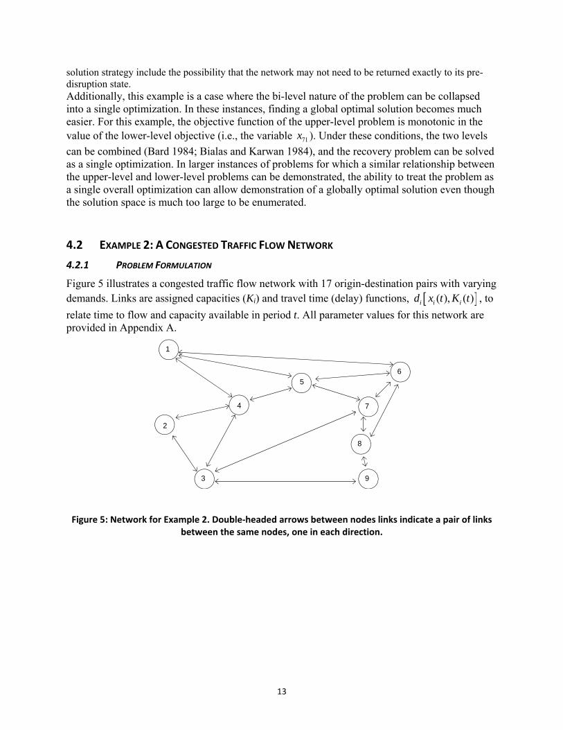
Figure 5 illustrates a congested traffic flow network with 17 origin-destination pairs with varying demands. Links are assigned capacities (Ki) and travel time (delay) functions, ( ), ( )i i id x t K t , to

relate time to flow and capacity available in period t. All parameter values for this network are provided in Appendix A.

Figure 5: Network for Example 2. Double‐headed arrows between nodes links indicate a pair of links between the same nodes, one in each direction. 

1

4

2

3 9

8

7

6

5

14 

Link flows xi are assumed to represent a deterministic user equilibrium, in which individual users choose paths through the network to minimize their own travel time. At time t, when the link capacities are Ki(t), this flow pattern is the solution of an optimization problem:

min ( )

0

, ( )ix t

i i i i rs rsi rs

d w K t dw e (18)

s.t. ( ) ( )i ip pp

x t f t i (19)

( ) ( ) ( )rsp p rs rs

p

f t e t q t rs (20)

0 ( ) ( )i ix t K t (21)

( ) 0pf t (22)

where ( )rsq t = units of desired flow from origin r to destination s in period t

( )rse t = units of unmet demand from origin r to destination s in period t

rs = unit cost of unmet demand from origin r to destination s

( )pf t = flow on path p for period t

ip = 1 if path p crosses link i; 0 if not rsp = 1 if path p connects origin r to destination s; 0 if not.

As with Example 1, the analytical team poses (18) – (22) under the recovery optimization formulation described in Section 3.3. The team simulates the disruption and recovery process with the following assumptions:

1. The disruption (at time 0) reduces the capacities of links 3-7, 7-3, 7-8, and 8-7 to 0.

2. For each pair of directional links, repair is represented by an eight-task activity-on-arc project network with precedence requirements (Figure 6).

3. Restoration of full capacity to a pair of directional links occurs at the milestone indicated by node

F (i.e., completion of all eight tasks). Forty percent of capacity restoration (for both directions) is achieved at the milestone represented by node C.

4. Tasks require varying amounts of two resources, each of which is available in limited quantity. For the first 10 periods after the disruption, 4 units of each resource are available. After the tenth period, additional resources can be acquired and the availability increases to 6 units of each resource. These resources must be shared between the two repair efforts.

5. The precedence structure of the repair projects for both pairs of links is the same, but the task

durations, resource requirements, and costs are different for the two sites. Table 3 indicates the task characteristics for the two projects. In each project, tasks 5 and 6 can be performed in one of two possible modes, with different durations, resource requirements, and costs. For later notational convenience, each of the link-task-mode (ijm) combinations in Table 3 has been assigned an index. This makes the formal statement of the recovery optimization problem easier.

15 

Figure 6: Link restoration project tasks and precedence for each pair of disrupted links  

(between nodes 3 and 7 and between nodes 7 and 8) 

Table 3: Recovery project characteristics for Example 2 

Index  Links Task 

Number Mode 

Duration (periods) 

Cost Resource Requirements (units) 

Resource 1  Resource 2 

1 

3‐7 and 7‐3 

1  1  4  80  2  0 

2  2  1  4  320  2  3 

3  3  1  6  300  1  2 

4  4  1  3  90  1  1 

5  5  1  4  160  2  1 

6  5  2  2  180  3  2 

7  6  1  7  420  2  2 

8  6  2  4  480  4  4 

9  7  1  4  200  3  1 

10  8  1  3  30  1  0 

11 

7‐8 and 8‐7 

1  1  3  60  2  0 

12  2  1  4  240  2  2 

13  3  1  4  200  1  2 

14  4  1  2  60  1  1 

15  5  1  3  180  2  2 

16  5  2  2  200  4  3 

17  6  1  5  300  2  2 

18  6  2  3  360  4  4 

19  7  1  3  150  3  1 

20  8  1  2  20  1  0 

This example is far more complex than Example 1. Example 2 illustrates several of the difficult resource allocation issues that may be faced in recovery planning for transportation (or other infrastructure) networks. In particular, this example includes:

More complicated precedence requirements on repair tasks

Repairs that affect multiple directional links simultaneously

Multiple modes for some of the tasks

A

B

C F

E

D1

2

3

4

5

6

7

8

16 

Intermediate milestones at which partial capacity is restored

Multiple resources that are constrained and used in different quantities by the various tasks and modes

Varying resource availability over the planning horizon.

This example also illustrates a more complex connection between the network flow determination and the evaluation of SI than is present in Example 1. Because the full statement of the recovery optimization for Example 2 is relatively long, it is presented as Appendix B. It should be noted for this optimization, the cost function Hi[xi(t)] (in eq. 4) is the total travel

time for all users of link i: i.e., ( ) ( ) ( ), ( )i i i i i iH x t x t d x t K t . The demands in Appendix A are

assumed to be constant, so ( )rsq t may be simplified to rsq .

4.2.2 SOLUTION 

For undisrupted conditions, all demand is met with the total vehicle-hours of travel equal to 8068. Table 4 lists the equilibrium link volumes. Note that the total volume on links between nodes 3 and 7 (~3200) is much larger than that on links between modes 7 and 8 (~700). This difference is important in determining the optimal recovery sequence.

Table 4: Equilibrium link volumes for nominal case in Example 2 

Link  Volume  Link  Volume  Link  Volume 

1‐4  0  4‐2  1860  6‐8  1202 

1‐5  622  4‐3  118  7‐3  1682 

1‐6  1838  4‐5  1761  7‐5  453 

2‐3  0  5‐1  196  7‐6  1139 

2‐4  830  5‐4  1978  7‐8  428 

3‐2  0  5‐6  1955  8‐6  137 

3‐4  931  5‐7  428  8‐7  283 

3‐7  1539  6‐1  1704  8‐9  340 

3‐9  850  6‐5  1721  9‐3  560 

4‐1  0  6‐7  1112  9‐8  80 

Immediately following the disruption, 195 units of demand are unmet and network flows result in 12,019 vehicle-hours of travel. When the analysts assign 10rs for all origin-destination pairs, the contribution

to SI while this initial condition persists is 12,019 – 8068 + 10 (195) = 5901 per period. This example illustrates the efficiency of the modifications this team introduced to Boctor’s (1996) simulated annealing method. In this example, only nine different combinations of capacity conditions affect the SI calculation:

No capacity on the disrupted links,

Forty percent capacity on links 3-7 and 7-3 and zero capacity on links 7-8 and 8-7,

Forty percent capacity on 7-8 and 8-7 and zero capacity on links 3-7 and 7-3,

17 

Forty percent capacity on all disrupted links,

Forty percent capacity on links 3-7 and 7-3 and 100% capacity on links 7-8 and 8-7,

Forty percent capacity on 7-8 and 8-7 and 100% capacity on links 3-7 and 7-3,

One hundred percent capacity on links 3-7 and 7-3 and zero capacity on links 7-8 and 8-7,

One hundred percent capacity on 7-8 and 8-7 and zero capacity on links 3-7 and 7-3, and

One hundred percent capacity on all disrupted links, The SI computations for different sequences are related to when the shifts in capacity occur, but that calculation is very simple. Hence, adding the memorization capability to the simulated annealing process radically decreases computational time for this example. The following recovery solution sequences illustrate how the dominance modification further reduces computations. The analysts summarize 3 recovery solution sequences using task indices from Table 3. Each solution has 16 elements (8 per node linked to node 7) and includes choices of 5 or 6, 7 or 8, 15 or 16, and 17 or 18, to reflect the choice of mode on the tasks that have multiple modes available. For purposes of the current discussion, it is useful to focus on three particular sequences:

1. [2 11 14 1 13 3 6 4 16 12 19 8 17 9 10 20]

2. [1 2 4 6 13 11 3 14 16 9 12 8 17 10 19 20]

3. [1 2 6 7 4 3 9 11 16 10 12 17 13 14 19 20].

Sequence 1 is the solution generated by a standard resource-constrained multimode scheduling procedure that minimizes the completion time for all tasks. The total time to completion is 23 periods. Forty percent of capacity is restored to links 7-3 and 3-7 at time 10; 40% of capacity is restored to links 7-8 and 8-7 at time 16; and all repairs and capacity restoration (for both sets of links) are completed at time 23 (Figure 7). SI is 78,738. Repair costs using the chosen modes are 2910. Analysts set 10 for the TRE weight, so the total objective value (eq. 1) for this solution is 107,838.

Table 4: Equilibrium link volumes for nominal case in Example 2 

Link  Volume  Link  Volume  Link  Volume 

1‐4  0  4‐2  1860  6‐8  1202 

1‐5  622  4‐3  118  7‐3  1682 

1‐6  1838  4‐5  1761  7‐5  453 

2‐3  0  5‐1  196  7‐6  1139 

2‐4  830  5‐4  1978  7‐8  428 

3‐2  0  5‐6  1955  8‐6  137 

3‐4  931  5‐7  428  8‐7  283 

3‐7  1539  6‐1  1704  8‐9  340 

3‐9  850  6‐5  1721  9‐3  560 

4‐1  0  6‐7  1112  9‐8  80 

18 

Figure 7: Restoration for Repair Sequence 1. Systemic impact is represented by the shaded grey area.  

Sequence 2 is a different solution with completion time of 23 periods (Figure 8). From the perspective of a normal resource-constrained project scheduler, this sequence is an alternate optimal solution. Sequence 2 implies a different schedule of tasks than sequence 1 and completes the partial repair of links 3-7 and 7-3 at time 6, rather than at time 10. The choices of modes for the multimode tasks are the same as in sequence 1, and the milestones for this sequence remain in the same order. SI is 61,538, so the overall objective function value is 90,638.

Figure 8: Restoration for Repair Sequence 2. Systemic impact is represented by the shaded grey area. 

The second sequence illustrates two important points. First, it illustrates the dominance concept discussed earlier. The order of the milestones in sequence 2 is the same as in sequence 1, but in sequence 2 one of those milestones (40% restoration of capacity for links 3-7 and 7-3) occurs earlier and none occur later; thus sequence 2 dominates sequence 1. Second, although sequences 1 and 2 appear equally desirable to a regular project scheduler, the SI quantities differ and thus the solutions are quite different for purposes of

19 

evaluating recovery after a network disruption. This difference illustrates the motivation for considering alternatives to traditional project scheduling approaches and developing the model formulation and solution method described in this paper. Sequence 3 is the solution determined for optimizing the recovery process.5 Although the overall recovery period is longer (25 periods), the SI value (53,654) is significantly less than the SI values for sequences 1 and 2 (Figure 9). Sequence (3) differs from the previous sequences in that it prioritizes complete capacity restoration for links 3-7 and 7-3 over partial capacity restoration of the other links. This strategy is effective for recovery optimization because the prioritized links are high volume links, so their prioritized restoration more rapidly decreases the cost of unmet demand and operations, resulting in a decreased SI. Under this sequence, the TRE value is 28,500, so the objective function value is 82,154. Thus, this solution achieves a reduction in both SI and TRE relative to the first two sequences, although it takes longer to complete. Because the overall duration is longer, this solution would not be considered optimal by traditional project scheduling procedures.

Figure 9: Restoration for Repair Sequence 3. Systemic Impact is represented by the shaded grey area. 

5 CONCLUSION  This paper introduces an optimization approach for identifying optimal recovery responses that maximize resilience for disrupted transportation networks. This work expands upon previous efforts by generalizing the optimization solution methodology to consider resource- constrained collections of recovery tasks.

5 The authors cannot guarantee this solution is optimal because there is no readily available way to solve the

optimization defined in Appendix B exactly. However, no attempts to improve upon it have been successful. Computation of this solution required about 135 seconds on a laptop computer. A strategy of finding an initial sequence using a standard resource-constrained scheduling algorithm (in this case, producing the solution labeled sequence 1 above) has been used, and the time required for that computation (3 seconds) is included in the total solution time.

20 

This methodology was applied to two networks for comparison with previous methods. The first application to a simple maximum flow network demonstrates that the approach is a more general formulation of the Henry and Ramirez-Marquez (2012) approach. The second example involves a more complex congested traffic flow network and recovery task sequencing. This example demonstrates the limitations of using more traditional project scheduling methods for recovery optimization. Specifically, this example shows that minimization of time to complete recovery tasks is an inadequate measure for recovery optimization. Using the new method’s objective function that considers network flows, costs of unmet demand, and recovery costs can find superior recovery sequences that would be considered suboptimal with traditional project scheduling approaches. This more complex objective function increases computational time, so the authors introduced memorization and dominance modifications to Boctor’s (1996) simulated annealing method that reduce computational requirements. This research focuses on how the network responds and evolves after a disruptive event. The next logical research and development area is the integration of system redesign with recovery responses to improve resiliency. This issue is a tri-level optimization problem. At the lowest level is an optimization to find flows in the network, given a current state of links/nodes. The next level up is the optimization of sequencing/allocating recovery resources, necessary to quantify resiliency. A third level adds opportunity for system redesign, including optimization of reconfiguring, adding, and/or redesigning pieces of the network to improve the achievable resiliency.

   

21 

7 REFERENCES  Alcaraz, J., C. Maroto, and R. Ruiz (2003). “Solving the Multimode Resource-Constrained Project Scheduling Problem with Genetic Algorithms,” Journal of Operational Research Society, 54, pp. 614-626. Bard, J.F. (1984). “Optimality Conditions for the Bilevel Programming Problem,” Naval Research Logistics Quarterly, 31, pp. 13-26. Bialas, W.F., and M.H. Karwan (1984). “Two-Level Linear Programming,” Management Science, 30:8, pp. 1004-1020. Bocchini, P., and D.M. Frangopol (2012). “Restoration of Bridge Networks after an Earthquake: Multicriteria Intervention Optimization,” Earthquake Spectra, 28:2, pp. 427-455. Boctor, F.F. (1996). “Resource-Constrained Project Scheduling by Simulated Annealing,” International Journal of Production Research, 34:8, pp. 2335-2351. Bouleimen, K., and H. Lecocq, “A New Efficient Simulated Annealing Algorithm for the Resource-Constrained Project Scheduling Problem and Its Multiple Mode Version,” European Journal of Operational Research, 149, pp. 268-281. Bruneau, M., S. Chang, R. Eguchi, G. Lee, T. O’ Rourke, A. Reinhorn, M. Shinozuka, K. Tierney, W. Wallace, and D. von Winterfeldt (2003). “A Framework to Quantitatively Assess and Enhance the Seismic Resilience of Communities,” Earthquake Spectra 19, pp. 737-38. Bush, G.W. (2002). “Homeland Security Presidential Directive-3 (HSPD-3),” Washington, D.C. Bush, G.W. (2003). “Homeland Security Presidential Directive-7 (HSPD-7),” Washington, D.C. Chang, S., and M. Shinozuka (2004). “Measuring Improvements in the Disaster Resilience of Communities,” Earthquake Spectra, 20, pp. 739-755. Chen, W.-N., J. Zhang, H. S.-H. Chung, R.-Z. Huang, and O. Liu (2010). “Optimizing Discounted Cash Flows in Project Scheduling – An Ant Colony Optimization Approach,” IEEE Transactions on Systems, Man and Cybernetics, Part C, 40:1, pp. 64-77. Chen, L., and E. Miller-Hooks (2012). “Resilience: An Indicator of Recovery Capability in Intermodal Freight Transport,” Transportation Science, 46(1), pp. 109-123. Clausen, J., A. Larsen, J. Larsen, and N. Rezanova. (2010). “Disruption management in the airline industry-Concepts, models and methods,” Computers and Operations Research, 37(5), pp. 809-821. Clinton, W. (1998). “Presidential Decision Directive PDD-63, Protecting America’s Critical Infrastructures,” Washington, D.C. Cutter, S.L., C.G. Burton, and C.T. Emrich (2010). "Disaster Resilience Indicators for Benchmarking Baseline Conditions," Journal of Homeland Security and Emergency Management, Vol. 7, Iss. 1, Article 51.

22 

Damak, N., B. Jarboui, P. Siarry, and T. Loukil (2009). “Differential Evolution for Solving Multi-Mode Resource-Constrained Project Scheduling Problems,” Computers & Operations Research, 36, pp. 2653-2659. Fiksel, J. (2003). “Designing Resilient, Sustainable Systems,” Environmental Science and Technology 37(23), pp. 5330-5339. Fisher, R. E., and M. Norman (2010). “Developing Measurement Indices to Enhance Protection and Resilience of Critical Infrastructures and Key Resources,” Journal of Business Continuity and Emergency Planning, 4(3), pp.191-206. Hartmann, S. (2001). “Project Scheduling with Multiple Modes: A Genetic Algorithm,” Annals of Operations Research, 102, pp. 111-135. Henry, D., and J.E. Ramirez-Marquez (2012). “Generic Metrics and Quantitative Approaches for System Resilience as a Function of Time,” Reliability Engineering and System Safety, 99, 114-122. Holling, C. (1973). “Resilience and Stability of Ecological Systems,” Annual Review of Ecology and Systematics 4 , pp. 1-23. Jarboui, B., N. Damak, P. Siarry, and A. Rebai (2008). “A Combinatorial Particle Swarm Optimization for Solving Multi-Mode Resource-Constrained Project Scheduling Problems,” Applied Mathematics and Computation, 195, pp. 299-308. Jozefowska, J., M. Mika, R. Rozychi, G. Waligora, and J. Weglarz (2001). “Simulated Annealing for Multimode Resource-Constrained Project Scheduling,” Annals of Operations Research, 102, pp. 137-155. Kolisch, R., and A. Drexl (1996). “Local Search for Nonpreemptive Multimode Resource-Constrained Project Scheduling,” IIE Transactions, 43, pp. 987-999. Luna, R., N. Balakrishnan, and C. Dagli. (2011). ”Postearthquake Recovery of a Water Distribution System: Discrete Event Simulation Using Colored Petri Nets.” J. Infrastruct. Syst., 17(1), 25–34. Mori, M., and C.C. Tseng (1997). “A Genetic Algorithm for Multimode Resource-Constrained Project Scheduling,” European Journal of Operational Research, 100, pp. 134-141. Obama, B. (2013). “Presidential Policy Directive 21: Critical Infrastructure Security and Resilience,” Washington, D.C. Ozdamar, L., (1999). “A Genetic Algorithm Approach to a General Category Project Scheduling Problem,” IEEE Transactions on Systems, Man and Cybernetics, Part C, 29:1, pp. 44-59. Park, J., T. P. Seager, P. S. C. Rao, M. Convertino, and I. Linkoz (2013). “Integrating Risk and Resilience Approaches to Catastrophe Management in Engineering Systems,” Risk Analysis, 33(3), pp. 356-366. Reagan, R. (1982). “Executive Order 13282, National Security Telecommunications Advisory Committee,” Washington, D.C. Rose, A. (2007). “Economic Resilience to Natural and Man-Made Disasters; Multidisciplinary Origins and Contextual Dimensions,” Environmental Hazards 7(4), pp. 383-398.

23 

Rose, A., and S.-Y. Liao (2005). “Modeling Regional Economic Resilience to Disasters: A Computable General Equilibrium Analysis of Water Service Disruptions,” Journal of Regional Science 45, pp. 75-112. Sempier, T.T., D.L. Swann, R. Emmer, S.H. Sempier, and M. Schneider ( 2010). Coastal Community Resilience Index: A Community Self-Assessment,accessed June 17, 2013 at http://www.masgc.org/pdf/masgp/08-014.pdf . Tierney, K., and M. Bruneau (2007). “Conceptualizing and Measuring Resilience: A Key to Disaster Loss Reduction,” TR News, May, pp. 14-17. TSA (Transportation Safety Administration) (2007). Transportation Systems Critical Infrastructure and Key Resources Sector-Specific Plan as Input to the National Infrastructure Protection Plan, Washington, D.C. Tseng, L.-Y., and S.-C. Chen (2009). “Two-Phase Genetic Local Search Algorithm for the Multimode Resource-Constrained Project Scheduling Problem,” IEEE Transactions on Evolutionary Computation, 13:4, pp. 848-857. Vugrin, E.D., D.E. Warren, M.A. Ehlen, and R.C. Camphouse (2010). “A Framework for Assessing the Resilience of Infrastructure and Economic Systems,” in Sustainable and Resilient Critical Infrastructure Systems: Simulation, Modeling, and Intelligent Engineering, Kasthurirangan Gopalakrishnan and Srinivas Peeta, eds., Springer-Verlag, Inc., New York. Vugrin, E.D., and R.C. Camphouse (2011). “Infrastructure resilience assessment through control design,” International Journal of Critical Infrastructures, 7:3, October, pp. 243-260. Wang, J., C. Qiao, and H. Yu. (2011). “On Progressive Network Recovery After a Major Disruption,” Proceedings of IEEE INFOCOM 2011, Shanghai, April 10-15, 2011. Xu, N., S.D. Guikema, R.A. Davidson, L.K. Nozick, Z. Çağnan, and K. Vaziri (2007). “Optimizing Scheduling of Post-Earthquake Electric Power Restoration Tasks,” Earthquake Engineering and Structural Dynamics, 36, pp. 265-284.

24 

Appendix A Data for Example 2 Network

Each directional link has a capacity, Ki, and a travel time (delay) function of the form (Davidson, 1966):

0, 1 ii i i i

i i

xd x K d J

K x

(A1)

Where:

,i i id x K = average travel time (delay) for a user when the flow is xi 0id = minimum travel time on link i

J = delay parameter

The parameters of the link delay functions for the Example 2 network are summarized in Table A-1. There are 17 origin-destination (O-D) pairs, with demand volumes as shown in Table A-2.

Table A‐1: Link parameters 

Link 

Capacity, K (each 

direction separately) 

Minimum Travel Time (min) 

J Parameter 

1‐4 and 4‐1  1800  16.0  0.12 

1‐5 and 5‐1  2400  16.8  0.08 

1‐6 and 6‐1  2400  26.4  0.08 

2‐3 and 3‐2  1200  21.6  0.15 

2‐4 and 4‐2  2400  10.8  0.08 

3‐4 and 4‐3  2400  12.0  0.08 

3‐7 and 7‐3  2400  22.8  0.08 

3‐9 and 9‐3  1800  33.6  0.12 

4‐5 and 5‐4  2400  8.4  0.08 

5‐6 and 6‐5  2400  13.2  0.08 

5‐7 and 7‐5  1800  12.8  0.12 

6‐7 and 7‐6  1200  6.0  0.08 

6‐8 and 8‐6  2400  9.6  0.08 

7‐8 and 8‐7  600  9.6  0.15 

8‐9 and 9‐8  2400  4.8  0.08 

25 

Table A‐2: Origin‐destination pairs and volumes for Example 2 

Origin Node 

Destination Node 

Volume 

1  6  1520 

1  8  940 

2  6  830 

3  6  2070 

3  7  400 

3  9  850 

6  1  1670 

6  2  1500 

6  3  1230 

6  8  350 

6  9  340 

7  2  280 

7  3  460 

8  1  230 

8  3  110 

9  2  80 

9  3  560 

Because the network links have limited capacities and the delay functions are only defined for flows less than capacity, it is possible that no feasible flow pattern on the network links will satisfy all the O-D demands. For the network data summarized above, there is a feasible assignment of all traffic to the network, but in the case of disruptions that reduce or remove some link capacity, feasibility may be lost. The approach used here for that situation is to add an artificial link for each O-D pair directly connecting the origin to the destination at a travel time equal to four times the minimum travel time for that O-D pair. These links have unlimited capacity. Thus, if there is insufficient capacity on the actual network links to handle all demand and the equilibrium congested travel time increases by a factor of 4 for a given O-D pair, the remainder of demand for that pair uses the artificial link and is reported as unmet demand.

26 

Appendix B Complete Formulation of the Optimization for Example 2

Using the index h for the recovery task ijm combinations, as indicated in Table 2 in the main text, the recovery optimization problem for Example 2 can be stated as shown in eqs. B1-B40. In the objective

function (B1), the constants 0iH that appear in the generic eq. 4 have been omitted because they do not

affect the optimization. The task costs hC in the objective function are the values shown in Table 2, and

the delay functions are from eq. A1. Constraints (B3)-(B6) enforce the requirement that only one mode can be chosen for the tasks that have two possible modes. The precedence constraints for the tasks have been written in extensive form in eqs. B7-B34 to be as clear as possible about how these constraints are constructed when there are multiple modes for some tasks.

To implement the increments to capacity at selected milestones, four dummy tasks are defined (h indices 21-24). Each of these tasks has zero duration, zero cost, and uses no resources. Their purpose is to create the milestone as a task with an initiation that corresponds to completion of a set of predecessors and a completion that allows the capacity increment to be implemented. Task indices 21 and 22 correspond to the milestones at nodes C in the two project diagrams, and task indices 23 and 24 correspond to completion of the two projects. The link indices used in constraints (B36)-(B39) correspond to the indices of the directional links in Table A-2 of Appendix A.

Min 1

( ) ( ), ( ) ( )T

i i i i rs rs h htt rs h

x t d x t K t e t C u

(B1)

s.t. 1

1 1, ...,T

htt

u h

(B2)

5 61 1

1T T

t tt t

u u

(B3)

7 81 1

1T T

t tt t

u u

(B4)

15 161 1

1T T

t tt t

u u

(B5)

17 181 1

1T T

t tt t

u u

(B6)

4 11 1

4T T

t tt t

t u t u

(B7)

5 11 1

4T T

t tt t

t u t u

(B8)

27 

6 11 1

4T T

t tt t

t u t u

(B9)

7 211 1

T T

t tt t

t u t u

(B10)

8 211 1

T T

t tt t

t u t u

(B11)

9 41 1

3T T

t tt t

t u t u

(B12)

10 31 1

6T T

t tt t

t u t u

(B13)

10 71 1

7T T

t tt t

t u t u

(B14)

10 81 1

4T T

t tt t

t u t u

(B15)

14 111 1

3T T

t tt t

t u t u

(B16)

15 111 1

3T T

t tt t

t u t u

(B17)

16 111 1

3T T

t tt t

t u t u

(B18)

17 221 1

T T

t tt t

t u t u

(B19)

18 221 1

T T

t tt t

t u t u

(B20)

19 141 1

2T T

t tt t

t u t u

(B21)

20 131 1

4T T

t tt t

t u t u

(B22)

20 171 1

5T T

t tt t

t u t u

(B23)

20 181 1

3T T

t tt t

t u t u

(B24)

28 

21 21 1

4T T

t tt t

t u t u

(B25)

21 51 1

4T T

t tt t

t u t u

(B26)

21 61 1

2T T

t tt t

t u t u

(B27)

22 121 1

4T T

t tt t

t u t u

(B28)

22 151 1

3T T

t tt t

t u t u

(B29)

22 161 1

2T T

t tt t

t u t u

(B30)

23 91 1

4T T

t tt t

t u t u

(B31)

23 101 1

3T T

t tt t

t u t u

(B32)

24 191 1

3T T

t tt t

t u t u

(B33)

24 201 1

2T T

t tt t

t u t u

(B34)

1

1, 2 ; 1,...,h

tk

h h kth t

r u R k t T

(B35)

8 21 231 1

( ) 960 1440t t

K t u u

(B36)

22 21 231 1

( ) 960 1440t t

K t u u

(B37)

25 22 241 1

( ) 240 360t t

K t u u

(B38)

27 23 241 1

( ) 240 360t t

K t u u

(B39)

0,1 1, ..., 24; 1, ...,htu h t T (B40)

29 

To evaluate the objective function (B1), the values of ( )ix t and ( )rse t are the values that solve the

optimization given in eqs. 18-22 in the main body of the paper. The problem specified by eqs. B1-B40 is the upper-level problem, which passes values of ( )iK t to the lower-level problem in eqs. 18-22. The

solution to the lower-level problem allows evaluation of the objective function in the upper-level problem.