Optimal routing problems and multimodularity - math.vu.nlsbhulai/publications/RR3727.pdf · de...

ISS

N 0

249-

6399

appor t de r e c herche

THÈME 1

INSTITUT NATIONAL DE RECHERCHEEN INFORMATIQUE ET EN AUTOMATIQUE

Optimal Routing Problemsand

Multimodularity

EitanAltman — SandjaiBhulai — BrunoGaujal — Arie Hordijk

N° 3727

June,1999

Optimal Routing Problemsand

Multimodularity∗

Eitan Altman† , Sandjai Bhulai‡ , Bruno Gaujal§ , Arie Hordijk¶

Thème 1 — Réseaux et systèmesProjet Mistral, Sloop

Rapport de recherche n° 3727 — June, 1999 — 25 pages

Abstract: In this paper we study the static assignment of packets to M parallel heteroge-neous servers with no buffers. Blocked packets are lost and the objective is to minimizethe average number of lost packets. The paper is divided into three parts. In the first partwe formulate the problem as a Markov Decision Problem with partial observation andwe derive an equivalent full observation problem. From this full observation problemwe derive some structural results. We establish, in particular, the existence of an optimalperiodic policy. The second part of the paper deals with computational aspects of theproblem. We use multimodularity to derive an algorithm to compute optimal policiesand show that for two servers the cost function is multimodular. In the third part weconsider the same problem with well known arrival processes, such as the Poisson Process,the Markov Modulated Poisson Process and the Markovian Arrival Process.

Key-words: Multimodularity, optimal control, partially observed Markov Decision Pro-cess, static routing.

∗ The research presented in this paper has been supported by the Van-Gogh grant N. 98001† INRIA, B.P. 93, 06902 Sophia Antipolis Cedex, France. E-mail: [email protected]‡ Vrije Universiteit, Faculty of Sciences, Amsterdam, The Netherlands. E-mail: [email protected]§ LORIA, B.P. 102, 54602 Villers-les-Nancy, France. E-mail: [email protected]¶ Leiden University, P.O. Box 9512, Leiden, The Netherlands. E-mail: [email protected]

Problèmes de routage optimal et multimodularité

Résumé : Dans cet article, nous étudions l’attribution statique des paquets à M serveursparallèles hétérogènes sans files d’attente. Les paquets bloqués sont perdus et l’objectif estde minimiser le nombre moyen de paquets perdus. Cet article est divisé en trois parties.Dans la première partie nous formulons le problème comme une chaîne de Markovcontrôlée avec observation partielle. Ensuite nous décrivons un problème équivalent avecobservation complet. De ce problème d’observation complet nous obtenons quelquesrésultats structurels. Nous montrons en particulier l’existence d’une politique optimalepériodique. La deuxième partie de cet article traite les aspects numériques du problème.Nous employons la multimodularité pour obtenir un algorithme qui calcule des stratégiesoptimales et nous montrons que la fonction de coût est multimodulaire pour le casde deux serveurs. Dans la troisième partie nous considérons le même problème avecquelques processus d’arrivée bien connus,tels que le processus de Poisson, le processusPoisson modulé et le processus d’arrivée Markovien.

Mots-clés : Multimodularité, contrôle optimal, chaîne de Markov contrôlée avec obser-vation partielle, routage statique.

Optimal Routing Problems and Multimodularity 3

1 IntroductionIn this paper we study the problem of optimal routing of arriving packets into a systemhaving a fixed number of servers and no queues. The objective is to maximize the through-put, or equivalently to minimize the losses, when the controller has no information onthe state of the servers. This problem can be classified as an open-loop optimal controlproblem. Similar problems have already been studied by Combé and Boxma [5], Rosbergand Towsley [18] and Koole [11]. However, exact results derived using these models de-pend on the assumption that the interarrival times of the arrival process are independentidentically distributed and on the assumption that the service times are exponentiallydistributed.

Hajek [8] introduced a novel approach to solve such problems in the context of queue-ing systems, based on multimodularity. Elementary properties of multimodular functionsand their relations with open-loop optimal control problems are further developed in Alt-man, Gaujal and Hordijk [1]. In Altman, Gaujal, Hordijk and Koole [2] a problem relatedto the one in this paper has been solved. Some multimodular and Schur convexity prop-erties of the costs were obtained, which enabled to give some characterizations of optimalpolicies.

In this paper we obtain new insight on the structure of optimal policies using tech-niques from Markov decision processes. We show that our problem has a remarkableand surprising Markovian structure, even though the arrival process is a general stationaryprocess. This allows us to establish the existence of optimal periodic policies. This impliesin fact that only a finite number of states are needed in the Markov Decision Process forsolving the problem.

We further obtain in this paper new multimodular properties as well as analyticalexpressions for the costs under general types of arrival processes (Poisson Process, MarkovModulated Poisson Process, Markovian Arrival Processes). We also study approaches forefficient numerical solutions of the control problem.

2 Optimal Routing to ServersIn this section we consider the problem of optimal routing of arriving packets into a systemwith a fixed number of servers having no waiting room. The servers work independentlyof each other and have service times, with general service distributions, independent ofthe arrival process. We assume that the process of interarrival times is stationary and thatthe controller has no information on the state of the servers. The objective in this settingis to maximize the expected throughput or equivalently to minimize the loss rate.

RR n° 3727

4 Altman, Bhulai, Gaujal, Hordijk

2.1 Problem FormulationConsider a system, to which packets arrive according to an arrival process (Tn)n∈N , whereTn represents the arrival epoch. We use the convention that T1 = 0 and we assume thatthe process (τn)n∈N of interarrival times τn = Tn+1−Tn is stationary, thus (τm, . . . , τm+h)and (τn, . . . , τn+h) are equal in distribution for all m , n and h.

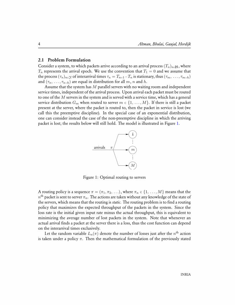
Assume that the system hasM parallel servers with no waiting room and independentservice times, independent of the arrival process. Upon arrival each packet must be routedto one of theM servers in the system and is served with a service time, which has a generalservice distribution Gm when routed to server m ∈ {1, . . . ,M}. If there is still a packetpresent at the server, where the packet is routed to, then the packet in service is lost (wecall this the preemptive discipline). In the special case of an exponential distribution,one can consider instead the case of the non-preemptive discipline in which the arrivingpacket is lost; the results below will still hold. The model is illustrated in Figure 1.

arrivals π

.

.

.

.

.

.

1

m

M

Figure 1: Optimal routing to servers

A routing policy is a sequence π = (π1, π2, . . .) , where πn ∈ {1, . . . ,M} means that thenth packet is sent to server πn. The actions are taken without any knowledge of the state ofthe servers, which means that the routing is static. The routing problem is to find a routingpolicy that maximizes the expected throughput of the packets in the system. Since theloss rate is the initial given input rate minus the actual throughput, this is equivalent tominimizing the average number of lost packets in the system. Note that whenever anactual arrival finds a packet at the server there is a loss, thus the cost function can dependon the interarrival times exclusively.

Let the random variable Ln(π) denote the number of losses just after the nth actionis taken under a policy π. Then the mathematical formulation of the previously stated

INRIA


objective is to minimize the following quantity over the set of all routing policies.

lim supn→∞

1n

n∑i=1

EπLi(π). (1)

2.2 Markov Decision Problem with Partial InformationUsing an approach similar to Koole [11], we formulate the model under consideration asa Markov decision problem with partially observed states. This will allow us to show thatthere exists an optimal periodic policy in our general setting of stationary arrival processand general independent service times.

Let X = NM0 denote the state space. Let x = (x1, . . . , xM ) ∈ X . Then xm = 0

indicates that there is no packet at server m before the next decision. If xm > 0 thenthere is a packet present at server m and xm is the total number of arrivals that occurredat other servers since this packet arrived. We assume that the system is initially empty,thus the initial state is given by (0, . . . , 0). Let A = {1, . . . ,M} denote the action set,where action a ∈ A corresponds to sending the packet to server a. Let Sm be a randomvariable with distribution Gm , then define fm(n) by

fm(n) = P(Sm ≥ τ1 + · · · + τn). (2)

Note that fm(n) represents the probability that a packet did not leave server m during narrivals. Now the transition probabilities for the state components are given by

pm(xm, a, x′m) =

1, if xm = 0, a 6= m and x′m = 0fm(1), if xm = 0, a = m and x′m = 11 − fm(1), if xm = 0, a = m and x′m = 0fm(n + 1), if xm = n and x′m = n + 1 for n ∈ N

1 − fm(n + 1), if xm = n and x′m = 0 for n ∈ N

0, otherwise.

The direct costs are given by

c(x, a) =

{0, xa = 01, xa > 0.

The set of histories at epoch t of this Markov decision process is defined as the setHt = (X × A)t−1 × X . For a full state information Markov decision process, a policy

RR n° 3727


π is defined as a set of decision rules (π1, π2, . . .) with πt : Ht → A. Since we cannotobserve the state of the servers in the above problem formulation, we restrict the policiesto decision rules with πt : At−1 → A.

For each fixed policy π and each realization ht of a history, the random variable At isgiven by at = πt(ht). The random variable Xt+1 takes values xt+1 ∈ X with probabilityp(xt, at, xt+1). With these definitions the expected average cost criterion function C(π)is defined by

C(π) = lim supT→∞

E1T

T∑t=1

c(Xt, At). (3)

Let Π denote the set of all policies. The Markov decision problem is to find a policyπ∗ , if it exists, such that C(π∗) = min{C(π) |π ∈ Π}. This Markov decision model ischaracterized by the tuple (X ,A, p, c).

Note that when the interarrival times are i.i.d. and the service times are exponential,the transition probabilities only depend on the presence of a packet at the server, whereasin our model we have to record the time a packet spends at the server. Therefore themodel in Koole [11] uses the reduced state space {0, 1}M .

2.3 Markov Decision Problem with Full InformationThe standard approach to solve Markov decision problems with partial information is totransform these problems into equivalent Markov decision problems with full informa-tion. However, in general this transformation results in very big state spaces. Thereforealgorithms which solve such Markov decision problems are often of limited use, sincetheir complexity is very large and numerical results are difficult to obtain. In this sectionwe formulate a Markov decision model (X ,A, p, c) with full state information, whichhas the property that it is equivalent to the partial information model and yet allows fornumerical computation.

Let X =(N ∪ {∞}

)M be the state space. The mth component xm of x ∈ X denotesthe number of arrivals that occurred since the last arrival to server m. We assume that theinitial state in this case is (∞, . . . ,∞). Let A = A be the corresponding action space.The transition probabilities are now given by

p(x, a, x′) =

{1, if x′a = 1 and x′m = xm + 1 for all m 6= a

0, otherwise.

Let the direct cost c(x, a) = fa(xa) , where fa(∞) equals zero. Note that the policies inΠ are allowed to depend on Xt , since these random variables do not refer to the state

INRIA


of the servers. The expected average cost criterion C defines the full state informationMarkov decision problem. The next theorem shows that the previously defined modelsare equivalent.

Theorem 2.1: The models (X ,A, p, c) and (X ,A, p, c) are equivalent in the sense thatpolicies in the two models can be transformed into each other leading to the same per-formances. Furthermore optimal policies exist for both models and the expected averagecost of the optimal policies are equal.

Proof : Let π ∈ Π be an arbitrary policy. Define the string of actions (a1, a2, . . .) bya1 = π1 , a2 = π2(a1), . . .. Now define the function Γ : Π → Π such that π = Γ(π) isthe constant policy given by πt(ht) = at for all ht.

From the definition of xt it follows that the mth component of xt is equal to (xt)m =t − maxs{as = m} if such an s exists and infinity otherwise. Now it follows thatP((Xt)m = n

)is non-zero only if at−n = m. Therefore P

((Xt)m = n

)= fm

((xt)m

)for n = (xt)m and zero otherwise. Note that the expected cost only depends on themarginal probabilities. From the structure of the cost function and the transition proba-bilities it follows that E c(Xt, a) = fa

((xt)a

)= E c(Xt, a). From this fact it follows that

C(π) = C(Γ(π)

).

Let π ∈ Π be an arbitrary policy. Note that there is only one sample path ht , whichoccurs with non-zero probability, since the initial state is known and the transition prob-abilities are zero or one. Now define the equivalence relation ∼ on Π such that π ∼ π′ ifπt(ht) = π′t(ht). Now it directly follows that policies in the same class have the same cost.Furthermore it follows that the constant policy π′t for each t is a representative elementin the class, which is the image of a policy in Π.

At this point we know that if there exists an optimal policy for the full observationproblem, then there is also an optimal policy for the partially observed problem with thesame value. In order to prove the existence of an optimal policy for our expected averagecost problem, we first introduce the discounted cost:

V α(π, x) = Eπ

[ ∞∑t=1

αt−1C(Xt, At)].

The optimal discounted cost is defined as

V α(x) = min{V α(π, x) |π ∈ Π}.

A sufficient condition for the existence of optimal stationary policy for the expectedaverage cost is that

∣∣V α(x)− V α(z)∣∣ is uniformly bounded in α and x for some z , where

V α(x) represents the minimal α-discounted costs (Theorem 2.2, Chapter 5 of Ross [19]).

RR n° 3727


Note that using the same policy for different initial states can only lead to a differencein cost when a packet is sent to a server for the first time. Since 0 ≤ αt c(x, a) ≤ 1 it followsthat the difference in cost cannot be larger than M . Now let πz denote the α-optimalpolicy for initial state z and V α(πz, x) the value for the assignment done for initial statex using πz . Then

V α(x) − V α(z) ≤ V α(πz, x) − V α(z) = V α(πz, x) − V α(πz, z) ≤M.

The proof is completed by repeating the argument for V α(z) − V α(x) with πx.

Instead of describing a policy using a sequence π , it will sometimes be more helpful toconsider an equivalent description using time distances between packets routed to eachserver. More precisely, define for server m

ηm(0) = 0 and ηm(j) = min{i > ηm(j − 1) |πi = m},

for j ∈ N. Define the distance sequence δm by

δm = (δm1 , δm2 , . . .), with δmj = ηm(j) − ηm(j − 1),

for j ∈ N. In order to show that these quantities are well defined, we show that eachoptimal policy uses every server infinitely many times. In the sequel we drop the bar inthe notation, since we already established equivalence between the partial and full stateinformation model.

Theorem 2.2: Every optimal policy π = (π1, π2, . . .) has the property that every serveris used infinitely many times, thus sup{j |πj = m} =∞ for m ∈ {1, . . . ,M}.

Proof : Assume that there is a server m , which is not used infinitely many times. Thenthere is an N such that πj 6= m for all j ≥ N . Let π′ = (πN , πN+1, . . .). It followsthat the difference of the total expected costs until any time n with n > N between thepolicies π and π′ is at most M . Since the criterion function looks at the expected averagecost both policies have the same cost C(π) = C(π′).

Now choose n such that fm(n) < C(π′). Note that this is possible since the costincurred using an arbitrary policy is positive and since for all m , limn→∞ fm(n) = 0.Define the policy π′′ by

π′′j =

{m, if j is a multiple of n

π′j−bj/nc, otherwise.

INRIA


Note that the assignments for all j , which are not a multiple of n , are equal underboth π′ and π′′ , but occur later under π′′ and therefore c

(Xj+bj/nc(π′′), Aj+bj/nc(π′′)

)≤ c(Xj(π′), Aj(π′)

)for all j which are not a multiple of n. It follows that C(π′′) ≤

1nfm(n) + n−1

n C(π′). By definition of n it follows that C(π′′) < C(π′) , thus π′ is notoptimal. This leads to a contradiction, because it follows that π is not optimal either.

Theorem 2.3: Let fm(n) be strictly positive and decreasing to zero in n for all m. Thenthere exists an optimal periodic policy.

Proof : Let π be an arbitrary policy andm be an arbitrary server. Suppose that the distancesequence δ = δm for this server has the property that sup{δj | j ∈ N} = ∞. We shallconstruct a policy π′ with distance sequence δπ

′such that sup{δπ′j | j ∈ N} is finite and

C(π′) ≤ C(π).Let p = min{fm(k) − fm(k + 1) |m = 1, . . . ,M, k = 1, . . . ,M}. Note that p is

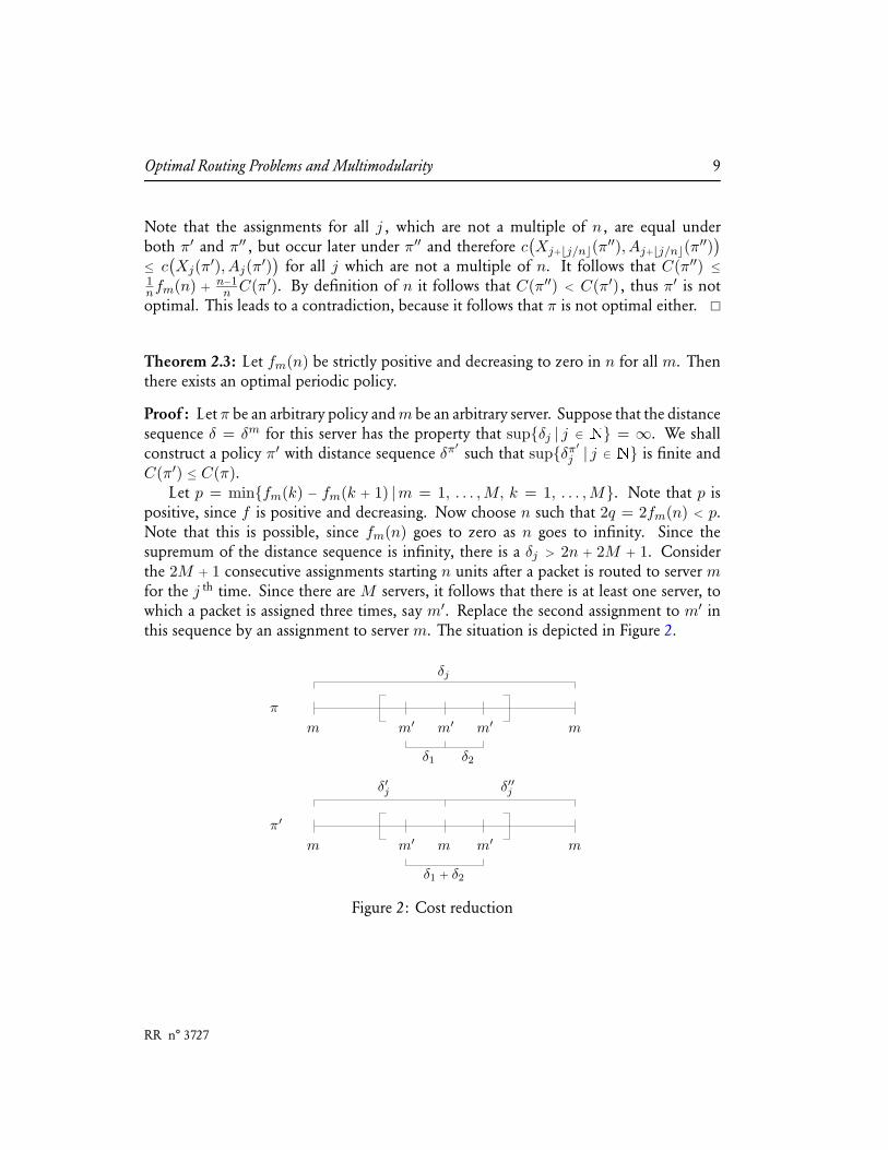
positive, since f is positive and decreasing. Now choose n such that 2q = 2fm(n) < p.Note that this is possible, since fm(n) goes to zero as n goes to infinity. Since thesupremum of the distance sequence is infinity, there is a δj > 2n + 2M + 1. Considerthe 2M + 1 consecutive assignments starting n units after a packet is routed to server mfor the j th time. Since there are M servers, it follows that there is at least one server, towhich a packet is assigned three times, say m′. Replace the second assignment to m′ inthis sequence by an assignment to server m. The situation is depicted in Figure 2.

π

δj

m m′ m′ m′ m

δ1 δ2

π′

δ′j δ′′j

m m′ m m′ m

δ1 + δ2

Figure 2: Cost reduction

RR n° 3727


We consider the decrease in the total expected cost until the lth instant, where l is anarbitrary integer larger than the time at which a packet is routed to server m for the j + 1sttime. This decrease is given by[

fm(δj) + fm′(δ1) + fm′(δ2)]−[fm(δ′j) + fm(δ′′j ) + fm′(δ1 + δ2)

]>[

fm(δj) + fm′(δ1) + fm′(δ2)]−[2fm(n) + fm′(δ1 + 1)

]=

fm(δj) + fm′(δ2) +[fm′(δ1) − fm′(δ1 + 1)

]−[2fm(n)

]>

fm(δj) + fm′(δ2) + p − 2q > 0.

The first inequality follows from the fact that n < δ′j , n < δ′′j , δ1 + δ2 ≥ δ1 + 1 and f isdecreasing. The second inequality follows from the definition of p. Since f is positive itfollows by construction of n that the last inequality holds.

Repeating this procedure for every δj > 2n + 2M + 1 provides us a policy π′ suchthat C(π′) ≤ C(π) and sup{δπ′j | j ∈ N} < 2n + 2M + 1. By repeating this procedure forevery server, we get an optimal policy that visits a finite number of states. By Chapter 8 ofPuterman [17] we know that the optimal policy can be chosen stationary. It follows thatπn(hn) = π0(xn). Since the state transitions are deterministic it follows that the optimalpolicy is periodic.

From (2) it follows that fm(n) satisfies the conditions in the previous theorem, sincethe random variables τn are positive. Therefore we know that the optimal policies areperiodic. In the next section we will show how we can use this result in order to usemultimodularity to find optimal routing policies.

2.4 Optimal Routing to Two ServersIn the previous section we showed that the optimal policy for all stationary arrival processesis periodic. In the case that there are only two servers in the system, we can say moreabout the structure of the optimal policy, using the fact that there is a full state informationMarkov decision process for this model.

In Liu and Towsley [13] it is pointed out that when the system has identical servers,thus the service distributions of the servers are equal, then the round robin policy is optimal,which means that sending a packet to each server alternatively is optimal. The next theoremshows that for two servers with exponential service times the optimal periodic policy issending the first packet to the slowest server and then several packets to the fastest server.

Theorem 2.4: Suppose that the two servers have service times, which are exponentiallydistributed with rates µ1 and µ2 respectively such that µ1 < µ2. Then the optimal policyhas the form (1, 2, . . . , 2)∞.

INRIA


Proof : By Theorem 2.2 we know that all the servers are used infinitely many times. Thusthe assignment to server 1 and consecutively to server 2 occurs infinitely many times.By Theorem 2.1 we know that the state after these occurrences are equal. Therefore theassignments between these occurrences must equal too. Now it immediately follows thatthere is an optimal policy of the form π = (1, . . . , 1, 2, . . . , 2).

Now suppose that the number of 1’s and 2’s in such a policy are given by a and brespectively. Let n = a + b , then C(π) is given by nC(π) = (a − 1)f1(1) + f1(b + 1) +

(b − 1)f2(1) + f2(a + 1). Let the policy π′ be the policy where the first 1 is interchangedwith the last 2. Then nC(π′) = (a−2)f1(1) +f1(b) +f1(2) + (b−2)f2(1) +f2(a) +f2(2).Now n [C(π)−C(π′)] =

{[f1(b+ 1)− f1(b)

]−[f1(2)− f1(1)

]}+{[f2(a+ 1)− f2(a)

]−[

f2(2)−f2(1)]}

. From the convexity of fm(n) in n it follows that the previous quantity ispositive. Therefore the form of the optimal policy is either (1, 2, . . . , 2) or (2, 1, . . . , 1).Since µ1 < µ2 and therefore f1(n) > f2(n) for all n ∈ N , it follows that (1, 2, . . . , 2) isthe optimal policy.

3 MultimodularityMultimodularity was introduced by Hajek [8] for the study of admission control in queue-ing systems. The study focused on the assignment of a sequence of arrivals at a controller,who has to assign a certain fraction to an infinite queue. Hajek proved, by using multi-modularity, that the optimal assignment has some regular structure, where the objectiveis to minimize the expected number of customers in the queue.

In this section we define multimodularity and study some properties of this concept.Furthermore we show that multimodularity provides us with a method to compute optimalrouting policies. In particular we shall prove that in case we have two servers in the system,the cost function is multimodular.

3.1 General PropertiesLet Z be the set of integers. Let ei ∈ Zn for i = 1, . . . , n denote the vector havingall entries zero except for a 1 in the i th entry. Let di be given by di = ei−1 − ei fori = 2, . . . , n. Then the base of vectors for multimodularity is defined as the collection

RR n° 3727


B = {b0 = −e1, b1 = d2, . . . , bn−1 = dn, bn = en}. Thus we have

b0 = ( −1, 0, 0, · · · 0, 0, 0 )b1 = ( 1, −1, 0, · · · 0, 0, 0 )b2 = ( 0, 1, −1, · · · 0, 0, 0 )...

......

......

bn−2 = ( 0, 0, 0, · · · 1, −1, 0 )bn−1 = ( 0, 0, 0, · · · 0, 1, −1 )bn = ( 0, 0, 0, · · · 0, 0, 1 ).

Following Hajek, a function g defined on Zn is called multimodular if for all x ∈ Zn andbi , bj ∈ B with i 6= j

g(x + bi) + g(x + bj) ≥ g(x) + g(x + bi + bj). (4)

Let g be a function onZn. Define ∆eig(x) = g(x+ei)−g(x) for all x ∈ Zn. Since the unitvectors form a basis of Zn , every vector v is a linear combination of the unit vectors andcan be written like v =

∑ni=1 λi ei. Then ∆v is defined as ∆vg(x) =

∑ni=1 λi ∆eig(x).

These definitions provide a useful characterization for multimodularity.

Lemma 3.1: ([1], Lemma 2.2) A function g is multimodular if and only if

∆v∆wg ≤ 0,

for all v, w ∈ B with v 6= w.

In future discussions we need more than multimodularity with respect to a base B only.It is often needed that the same function is also multimodular with respect to the base−B. From the linearity of the operator ∆ and Lemma 3.1 it immediately follows that g isalso multimodular with respect to −B.

3.2 ConvexityWe define the notion of an atom in order to study some properties of multimodularity.In Rn the convex hull of n + 1 affine independent points in Zn forms a simplex. Thissimplex, defined on x0, . . . , xn is called an atom if for some permutation σ of (0, . . . , n)

x1 = x0 + bσ(0),

x2 = x1 + bσ(1),...

......

xn = xn−1 + bσ(n−1),

x0 = xn + bσ(n).

INRIA


This atom is referred to as A(x0, σ) and the points x0, . . . , xn are called the extreme pointsof this atom. Each unit cube is partitioned into n! atoms and all atoms together tile Rn.We can use this to extend the function g : Zn → R to the function g : Rn → R asfollows. If x ∈ Zn then define the function by g(x) = g(x). Thus g agrees with g onZn. If x is not an extreme point of an atom, then x is contained in some atom A. The

value of g on such a point x ∈ Rn is obtained as the corresponding linear interpolationof the values of g on the extreme points of A. The following theorem shows the relationbetween multimodularity and convexity.

Theorem 3.2: ([8],[1], Theorem 2.1, [4]) A function g is multimodular if and only if thefunction g is convex.

We defined multimodularity on the set of integers. Remark 2.1 of Altman, Gaujal andHordijk [1] points out that for any convex subset S , which is a union of a set of atoms,multimodularity of g and convexity of g still holds when restricted to S. Multimodularityon this convex subset means that (4) must hold for all x ∈ S and bi , bj ∈ B with i 6= j ,such that x+bi , x+bj and x+bi+bj ∈ S. We will see that this is essential for the applicationin the next sections, where we use the set S = N

n0 , with N0 = N ∪ {0} = {0, 1, 2, . . .}.

From the previous discussion it follows that multimodularity has a relation with con-vexity. In the next section we show how we can exploit this relation in order to minimizeconvex functions on the lattice.

3.3 Local SearchLet g : Zn → R be an objective function in a mathematical model which has to beminimized. In general this is a hard problem to solve. In this section we show that if thefunction g is multimodular, then we can use a local search algorithm, which converges tothe globally optimal solution. In Koole and Van der Sluis [12] the local search algorithmhas been proven for the search space Zn. The following theorem shows that it also holdsfor any convex subset, which is a union of a set of atoms.

Theorem 3.3: Let g be a multimodular function on S , a convex subset which is a unionof atoms. A point x ∈ S is a global minimum if g(x) ≤ g(y) for all y 6= x such that xand y are both extreme points of an atom in S.

Proof : Let x ∈ S be a fixed point. Now suppose that there is a z ∈ Rn such that x+z ∈ Sand g(x+ z) < g(x) = g(x). We show that there is an atom A(x, σ) in S with an extremepoint y such that g(y) < g(x).

RR n° 3727


Since any n vectors of B form a basis of Rn , we can write z as z =∑n

i=0 βi bi.Furthermore, this can be done such that βi ≥ 0 , since any βi bi with βi < 0 can bereplaced by −βi

∑nj=0,j 6=i bj .

Now reorder the elements of B as (b′0, . . . , b′n) and the elements (β0, . . . , βn) as

(β′0, . . . , β′n) such that β′0 ≥ · · · ≥ β′n ≥ 0 and z =

∑ni=0 β

′i b′i. Note that this notation

is equivalent to the notation z = β′′0 b′0 + β′′1 (b′0 + b′1) + · · · + β′′n (b′0 + · · · + b′n) with all

β′′i ≥ 0 and with b′0 + · · · + b′n = 0. Now fix a non-zero point z′ = α z with α < 1 suchthat α (β′′0 + · · · + β′′n−1) ≤ 1. The set S is convex with x , x + z ∈ S , hence x + z′ ∈ S.Since by Theorem 3.2 g is convex and g(x + z) < g(x) , it follows that g(x + z′) < g(x).

Let σ be the permutation induced by (β′′0 , . . . , β′′n). Now consider the atom A(x, σ) ,

then by construction x + z′ ∈ A(x, σ). Since x is an extreme point and g is linear, theremust be another extreme point, say y , such that g(y) < g(x).

This theorem shows that to check whether x is a globally optimal solution, it is sufficientto consider all extreme points of all atoms with x as an extreme point. When a particularextreme point of such an atom has a lower value than x , then we repeat the same algorithmwith that point. Repeating this procedure is guaranteed to lead to the globally optimalsolution.

Every multimodular function is also integer convex (see Theorem 2.2 in [1]). Onecould wonder if local search also works with integer convexity instead of multimodularity,which is a stronger property. The next counter-example in ({0, 1, 2})2 shows that this isnot true and that multimodularity is indeed the property needed for using local search.Define the function g such that

g(0, 2) = −1, g(1, 2) = 2, g(2, 2) = 5,g(0, 1) = 2, g(1, 1) = 1, g(2, 1) = 0,g(0, 0) = 5, g(1, 0) = 4, g(2, 0) = 3.

One can easily check that g is an integer convex function, but not multimodular sinceg((1, 2) + b0

)+ g((1, 2) + b2

)= 0 < 4 = g

((1, 2)

)+ g((1, 2) + b0 + b2). Starting the

local search algorithm at coordinate (2, 1) shows that all neighbors have values, which aregreater than 0. However, the global minimum is g

((0, 2)

)= −1.

Since all the extreme points of all atoms with x as an extreme point can be writtenas x +

∑ni=0 αi bi with αi ∈ {0, 1} , bi ∈ B , the neighborhood of a point x consists of

2n+1 − 2 points (we subtract 2 because when αi = 0 or when αi = 1 for all i , then thepoints coincide).

Although the complexity of the local search algorithm is big for large n , the algorithmis worthwhile studying. First of all, comparing to minimizing a convex function on the

INRIA


lattice, this algorithm gives a reasonable improvement. Secondly, the algorithm can serveas a basis for heuristic methods.

In the next section we show that the cost function in the model with only two serversis multimodular.

3.4 Optimal Routing to Two ServersIn the previous section we showed that the optimal policy for all stationary arrival processesis periodic. In this case the notation of the distance sequence can be beneficially usedto approach the decision problem. After the first assigment to server m , the distancesequence δm for server m is periodic, say with period d(m). Since the servers are idleinitially, the first assignment does not lead to a loss of a packet. Therefore in futurediscussions we will write π = (π1, . . . , πn) for the periodic assignment sequence withperiod n and with a slight abuse of notation we denote the periodic distance sequence forserver m by δm = (δm1 , . . . , δ

md(m)).

The periodicity reduces the cost function in complexity. Since we use the expectedaverage number of lost packets as the cost function, we only have to consider the costsincurred during one period. The cost function for server m is given by

gm(π) =1n

d(m)∑j=1

fm(δmj ). (5)

The expected average number of lost packets in the total system is then given by

g(π) =M∑m=1

gm(π) =1n

M∑m=1

d(m)∑j=1

fm(δmj ). (6)

Note that equation (1) or equivalently (3) are exactly given by equation (6). It is tempting toformulate that gm(π) is multimodular in π for allm. Note that this is not necessarily true,since an operation v ∈ B applied to π leads to different changes in the distance sequencesfor different servers. In the case where we have two servers, we can prove multimodularityhowever, since an operation applied to the first server, leads to an opposite operationapplied to the second server.

In the next discussion we assume that we have two servers and that π is a periodicsequence with period n. We will show that (6) is multimodular in π. After establishingmultimodularity of the cost function for two servers, we can use the local search algorithmto find optimal policies for different server rates. In order to prove the multimodularity

RR n° 3727


we do not use (5), but instead we use g′m(π) defined by

g′m(π) =1n

d(1)∑j=1

fm(δ1j ). (7)

This function only looks at the distance sequence assigned to the first queue. Note thatg(π) can now be expressed as g(π) = g′1(π) + g′2(~3 − π). We first prove that g′m(π) ismultimodular in π.

Lemma 3.4: Let π be a fixed periodic policy with period n. Let g′m(π) be defined as in(7). Then g′m(π) is a multimodular function in π.

Proof : Since π is a periodic sequence, the distance sequence δ = δ1 is also a periodicfunction, say with period p = d(1). Now, define the function hj for j = 1, . . . , p byhj(π) = fm(δj). The function hj represents the cost of the (j + 1)st assignment bylooking at the j th interarrival time. We will first prove that this function is multimodularfor V = {b1, . . . , bn−1}.

Let v , w ∈ V with v 6= w. If none of these elements changes the length of thej th interarrival time then hj(π) = hj(π + v) = hj(π + w) = hj(π + v + w). Supposethat only one of the elements changes the length of the interarrival time, say v , thenhj(π + v) = hj(π + v + w) and hj(π) = hj(π + w). In both cases the function hj(π)satisfies the conditions for multimodularity.

Now suppose that v adds and w decreases the length of the j th interarrival time byone. Then hj(π + v) ≤ hj(π) = hj(π + v + w) ≤ hj(π + w). Since hj is a convexdecreasing function, it follows that hj(π +w) − hj(π + v +w) ≥ hj(π) − hj(π + v). Nowthe multimodularity condition in equation (4) directly follows by rearranging the terms.Since g′m(π) is a sum of hj(π) it follows that g′m(π) is multimodular for V .

Now consider the elements b0 and bn and note that the application of b0 and bn to πsplits an interarrival period and merges two interarrival periods respectively. Therefore

n g′m(π + b0) = n g′m(π) − fm(δ1) − fm(δp) + fm(δ1 + δp),n g′m(π + bn) = n g′m(π) − fm(δp) + fm(δp − 1) + fm(1),

n g′m(π + b0 + bn) = n g′m(π) − fm(δ1) − fm(δp) + fm(δ1 + 1) + fm(δp − 1).

Nown[g′m(π+b0)+g′m(π+bn)−g′m(π)−g′m(π+b0+bn)

]=[fm(δ1+δp)+fm(1)

]−[fm(δ1+

1) + fm(δp)]. Let k = δ1 + δp + 1. Since the function fm(x) + fm(y) with x + y = k is a

symmetric and convex function, it follows from Proposition C2 of Chapter 3 of Marshall

INRIA


and Olkin [15], that fm(x) +fm(y) is also Schur-convex. Since (δ1 + 1, δp) ≺ (δ1 + δp, 1) ,the quantity above is non-negative.

In the case that we use w = b0 and v ∈ V such that v does not alter δ1 , then it followsthat g′m(π + v + w) = g′m(π + v) + g′m(π + w) − g′m(π). The same holds for w = bnand v ∈ V such that v does not alter δp. Suppose that v does alter δ1 , then we haven[g′m(π + b0) + g′m(π + v) − g′m(π) − g′m(π + b0 + v)

]=[fm(δ1 + δp) + fm(δ1 − 1)

]−[

fm(δ1 + δp−1) +fm(δ1)]. When v alters δp we have n

[g′m(π+ bn) +g′m(π+v)−g′m(π)−

g′m(π + bn + v)]

=[fm(δp + 1) + fm(l)

]−[fm(δp) + fm(l + 1)

]for some l < δp. Now

by applying the same argument as in the case of b0 and bn we derive multimodularity ofg′m(π) for the base B.

Now we will prove that g(π) , which is given by g(π) = g′1(π)+g′2(~3−π) is multimodular.The proof is based on the fact that if a function is multimodular with respect to a base B ,then it is also multimodular with respect to −B.

Theorem 3.5: Let g′1 and g′2 be multimodular functions. Then the function g(π) givenby g(π) = c1 g

′1(π) + c2 g

′2(~3 − π) for positive constants c1 and c2 is multimodular in π.

Proof : Let v , w ∈ B , such that v 6= w. Then

g(π+v) + g(π + w)

= c1 g′1(π + v) + c2 g

′2(~3 − π − v) + c1 g

′1(π + w) + c2 g

′2(~3 − π − w)

= c1

[g′1(π + v) + g′1(π + w)

]+ c2

[g′2(~3 − π − v) + g′2(~3 − π − w)

]≥ c1

[g′1(π) + g′1(π + v + w)

]+ c2

[g′2(~3 − π) + g′2(~3 − π − v − w)

]= c1 g

′1(π) + c2 g

′2(~3 − π) + c1 g

′1(π + v + w) + c2 g

′2(~3 − π − v − w)

= g(π) + g(π + v + w).

The inequality in the fourth line holds, since g′1 is multimodular with respect to B and g′2is multimodular with respect to −B.

4 Arrival ProcessesIn the previous sections we derived an expression for the structure of the optimal policy,provided that the arrival process has stationary interarrival times. However, we were notable to explicitly formulate an expression for the period of this policy. In this section weassume that the service times are exponentionally distributed with service rate µm and welook at some special cases of stationary arrival processes. We derive an explicit expressionfor the cost function, which will enable us to compute the optimal policy analyticallywhen all parameters are specified.

RR n° 3727


4.1 Poisson ProcessConsider a Poisson process with rate λ. The process of interarrival times of this Poissonprocess is independent identically distributed with probability density f(t) = λ exp (−λt).Therefore it follows that (2) is given by

fm(n) = E exp

(−µm

n∑k=1

τk

)=[E exp (−µmτ1)

]n.

Note that the fact that the process of interarrival times is i.i.d. simplifies the cost function.Using the probability density of the interarrival times, the quantity between the bracketsin the right-hand side is given by

E exp (−µmτ1) =∫ ∞

0exp (−µmt)λ exp (−λt) dt =

λ

λ + µm.

Now it follows that the cost function is given by

g(π) =1n

M∑m=1

d(m)∑j=1

[λ

λ + µm

]δmj.

By choosing the Poisson process as the arrival process for our model, it becomes relativelysimple to calculate the optimal policies analytically. For example: suppose that we havea Poisson process with rate λ = 1 and suppose that the rate of the first server is µ1 = 1.We can study the behavior of the period of the optimal policy as we increase the rate ofthe second server µ2 ≥ µ1 as follows. Since the optimal policy is of the form (1, 2, . . . , 2)we can parameterize the cost function by the period n and the server speed µ2 given by

g(n, µ2) =1n

(12

)n+

1n

(1

1 + µ2

)2

+n − 2n

(1

1 + µ2

).

By solving the equations g(n, µ2) = g(n + 1, µ2) for n ≥ 2 we can compute the serverrates µ2 where the optimal policy changes. For example: the optimal policy changes from(1, 2) to (1, 2, 2) when µ2 ≥ 1+

√2. The results of the computation are depicted in Figure

3.

4.2 Markov Modulated Poisson ProcessThe MMPP [9] is constructed by varying the arrival rate of a Poisson process accordingto an underlying continuous time Markov process, which is independent of the arrival

INRIA


0 50 100 150 200 250 300 3502

3

4

5

6

7

8

9

10

µ2

perio

d

Figure 3: Relationship between n and µ2

process. Therefore let {Xn |n ≥ 0} be a continuous time irreducible Markov process withm states. When the Markov process is in state i , arrivals occur according to a Poissonprocess with rate λi. Let pij denote the transition probability to go from state i to state j.Then the infinitesimal generator Q is given by

Q =

−p1 p12 · · · p1m

p21 −p2 · · · p2m...

.... . .

...pm1 pm2 · · · −pm

, with pi =m∑j=1j 6=i

pij .

Let Λ = diag(λ1, . . . , λm) be the matrix with the arrival rates on the diagonal and λ =(λ1, . . . , λm) the vector of arrival rates. With this notation, we can use the matrix analyticapproach to derive a formula for (2).

Define the matrix F (t) is as follows. The elements Fij(t) are given by the conditionalprobabilities P(Xn+1 = j, τn+1 ≤ t |Xn = i) for n ≥ 1. It follows that F (∞) given by(Λ −Q)−1Λ is a stochastic matrix.

RR n° 3727


Theorem 4.1: (Section 5.3 in [16]) The sequence {(Xn, τn) |n ≥ 0} is a Markov renewalsequence with transition probability matrix F (t) given by

F (t) =∫ t

0e(Q−Λ)u duΛ =

[I − e(Q−Λ)t

](Λ −Q)−1Λ.

The MMPP is fully parameterized by specifying the initial probability vector q , the in-finitesimal generatorQ of the Markov process and the vector λ of arrival rates. Let the rowvector s be the steady state vector of the Markov process. Then s satisfies the equationssQ = 0 and se = 1 , where e = (1, . . . , 1). Define the row vector q by

q =1sλ· sΛ.

Then by Fisher and Meier-Hellstern [7] we know that q is the stationary vector of F (∞)and makes the MMPP interarrival process stationary. We can then use (2) to express thecost function for the MMPP. By Theorem 2.3 we know that the optimal policy is periodic.Therefore the cost is completely characterized by equations (5) and (6). If we assume thatthe underlying Markov chain of the MMPP is ergodic, it converges to the stationaryregime as t→∞ , and then the average cost is the same for any initial distribution.

In order to find an explicit expression for the cost function, we compute the Laplace-Stieltjes transform f∗(µ) of the matrix F . Since F is a matrix, we use matrix operationsin order to derive f∗(µ) , which will also be a matrix. The interpretation of the elementsf∗ij(µ) are given by E

[e−µτn+1 1{Xn+1=j} |Xn = i

]for n ≥ 1 , where 1 is the indicator

function. Let I denote the identity matrix, then f∗(µ) is given by

f∗(µ) =∫ ∞

0e−µItF (dt) =

∫ ∞0e−µIte(Q−Λ)t (Λ −Q)(Λ −Q)−1Λ dt

=∫ ∞

0e−(µI−Q+Λ)t dtΛ = (µI −Q + Λ)−1Λ.

In order to find an explicit expression for the cost function, we have to compute (2)first. This is done in the next lemma. Note that we do not need the assumption ofindependence of the interarrival times to derive this result.

Lemma 4.2: Let f∗(µ) be the Laplace-Stieltjes transform of F , where F is a transitionprobability matrix of a stationary arrival process. Then

fm(n) = E exp(−µ

n∑k=1

τk

)= q

[f∗(µ)

]ne.

INRIA


Proof : Define a matrix Qn with entries Qn(i, j) given by

Qn(i, j) = E

[exp

(−µ

n∑k=1

τk

)1{Xn=j}

∣∣∣∣X0 = i

].

Note that Q1 is given by f∗(µ). By using the stationarity of the arrival process it followsthat Qn(i, j) is recursively defined by

Qn(i, j) =m∑l=1

Qn−1(i, l) E[

exp(−µτn)1{Xn=j} |Xn−1 = l]

=m∑l=1

Qn−1(i, l) E[

exp(−µτ1)1{X1=j} |X0 = l]

=m∑l=1

Qn−1(i, l) ·Q1(l, j).

Note that the last line exactly denotes the matrix product, thus Qn = Qn−1 · Q1. Byinduction it follows that Qn = Qn1 . Then it follows that

fm(n) = E exp(−µ

n∑k=1

τk

)=

m∑i=1

m∑j=1

P(X0 = i)Qn(i, j) = q[f∗(µ)

]ne.

The last equation holds since the row vector q is the initial state of the Markov processand summing over all j is the same as right multiplying by e.

The previous lemma enables us to express the cost function (6) explicitly for the MMPP.The cost is now given by

g(π) =1n

M∑m=1

d(m)∑j=1

q[(µmI −Q + Λ)−1Λ

]δmj e.Note that although we know the structure of the optimal policy, it is not intuitivelyclear that it is optimal in the case of the MMPP. The following example will clarify thisstatement. Suppose that one has an MMPP with two states. Choose the rates λ1 andλ2 of the Poisson processes such that the policies would have period 2 and 3 respectivelyif the MMPP is not allowed to change state. One could expect that if the transitionprobabilities to go to another state are very small, the optimal policy should be a mixtureof both policies. But this is not the case as Theorem 2.4 shows.

RR n° 3727


4.3 Markovian Arrival ProcessThe Markovian arrival process model (MAP) is a broad subclass of models for arrivalprocesses. It has the special property that every marked point process is the weak limitof a sequence of Markovian arrival processes (see Asmussen and Koole [3]). In practicethis means that very general point processes can be approximated by appropriate MAP’s.The utility of the MAP follows from the fact that it is a versatile, yet tractable, family ofmodels, which captures both bursty inputs and regular inputs.

Markovian arrival processes can be modeled in a variety of ways. The model for theMAP described in Koole [10] has the advantage that the model is parameterized with fewparameters. In Chapter 10 of Dshalalow [6] it is shown that the MAP can be modeledsuch that it is a natural generalization of the Poisson process. Furthermore it is shownthat there is an analogous description for discrete PH-distributions. In this section we usethe model formulation described in Lucantoni, Meier-Hellstern and Neuts [14], whichreduces the computational complexity by using a matrix analytic approach. From thismodel it also easily follows that the MMPP is a special case of the MAP.

Model FormulationLet {Xn |n ≥ 0} be a continuous time irreducible Markov process with m states. As-sume that the Markov process is in state i. The sojourn time in this state is exponentiallydistributed with parameter γi. After this time has elapsed, there are two transition possi-bilities. Either the Markov process moves to state j with probability pij with generatingan arrival or the process moves to state j 6= i with probability qij without generating anarrival. With this definition it follows that

m∑j=1j 6=i

qij +

m∑j=1

pij = 1,

for all 1 ≤ i ≤ m. This definition also gives rise to a natural description of the modelin terms of matrix algebra. Define the matrix D with elements Dij = γi qij for i 6= j.Set the elements Dii equal to −γi. Define the matrix E with elements Eij = γi pij . Theinterpretation of these matrices is given as follows. The elementary probability that thereis no arrival in an infinitesimal interval of length dt when the Markov process moves fromstate i to state j is given by Dij dt. A similar interpretation holds for E , but in this case itrepresents the elementary probability that an arrival occurs. The infinitesimal generatorof the Markov process is then given by D + E. Note that the MMPP can be derived bychoosing D = Q − Λ and E = Λ.

In order to derive an explicit expression for the cost function, we use the same approachas in the case of the MMPP. The transition probability matrix F (t) of the Markov renewal

INRIA


process {(Xn, τn) |n ≥ 0} , given in Lucantoni, Meier-Hellstern and Neuts [14], is of theform

F (t) =∫ t

0eDu du =

[I − eDt

] (−D−1E

),

where again the elements Fij(t) of the matrix F (t) are given by P(Xn+1 = j, τn+1 ≤t |Xn = i) for n ≥ 1. It also follows that F (∞) defined by −D−1E is a stochastic matrix.Let the row vector s be the steady state vector of the Markov process. Then s satisfies theequations s(D + E) = 0 and se = 1. Define the vector row vector q by

q =1sEe

sE.

Then q is the stationary vector of F (∞). This fact can be easily seen upon noting thatsE = s(D + E − D) = s(D + E) − sD = −sD. With this observation it follows thatq F (∞) = (sEe)−1 sDD−1E = q. The MAP defined by q , D and E has stationaryinterarrival times. In this case we know that the optimal policy is periodic and the cost isthus completely determined by equations (5) and (6).

The Laplace-Stieltjes transform f∗(µ) of the matrix F is given by

f∗(µ) =∫ ∞

0e−µItF (dt) =

∫ ∞0e−µIteDt

(−D

)(−D−1

)E dt

=∫ ∞

0e−(µI−D)t dt E = (µI −D)−1E.

The interpretation of f∗ is given by the elements f∗ij(µ) , which represent the expectationE[eµτn+1 1{Xn+1=j} |Xn = i

]. By Lemma 4.2 we know that (2) is given by the product of

f∗. Therefore the cost function, when using the MAP as arrival process, is given by

g(π) =1n

M∑m=1

d(m)∑j=1

q[(µmI −D)−1E

]δmj e.References[1] E. Altman, B. Gaujal and A. Hordijk. Multimodularity, convexity and optimization

properties. Technical Report TW–97–07, Leiden University, 1997.

[2] E. Altman, B. Gaujal, A. Hordijk and G. Koole. Optimal admission, routing and ser-vice assignment control: the case of single buffer queues. Technical Report, INRIA,1998.

RR n° 3727


[3] S. Asmussen and G. Koole. Marked point processes as limits of Markovian arrivalstreams. Journal of Applied Probability , 30:365–372, 1993.

[4] M. Bartroli and S. Stidham, Jr., Towards a unified theory of structure of optimal poli-cies for control of network of queues. Technical report, Department of OperationsResearch, University of North Carolina, Chapel Hill, 1987.

[5] M.B. Combé and O.J. Boxma. Optimization of static traffic allocation policies.Theoretical Computer Science , 125:17–43, 1994.

[6] J.H. Dshalalow. Advances in Queueing: Theory, Methods and Open Problems. CRC Press,1995

[7] W. Fisher and K.S. Meier-Hellstern. The Markov-modulated Poisson process(MMPP) cookbook. Performance Evaluation, 18:149–171, 1992.

[8] B. Hajek. Extremal splitting of point processes. Mathematics of Operations Research ,10:543–556, 1985.

[9] H. Heffes and D.M. Lucantoni. A Markov modulated characterization of packetizedvoice and data traffic and related statistical multiplexer performance. IEEE Journalon Selected Areas in Communications , 4:856–868, 1986.

[10] G. Koole. Stochastic Scheduling and Dynamic Programming. PhD thesis, University ofLeiden, 1992.

[11] G. Koole. On the static assignment to parallel servers. IEEE Transactions on AutomaticControl , 1999. (to be published).

[12] G. Koole and E. van der Sluis. An optimal local search procedure for manpowerscheduling in call centers. Vrije Universiteit Amsterdam.

[13] Z. Liu and D. Towsley. Optimality of the round-robin routing policy. Journal ofApplied Probability , 31:466-475, 1994.

[14] D.M. Lucantoni, K.S. Meier-Hellstern and M.F. Neuts. A single-server queue withserver vacations and a class of non-renewal arrival processes. Advances in AppliedProbability , 22:675–705, 1990.

[15] A.W. Marshall and I. Olkin. Inequalities: Theory of Majorization and its Applications.Academic Press, 1979.

INRIA


[16] M.F. Neuts. Structured Stochastic Matrices of M/G/1 Type and their Applications. MarcelDekker, 1989.

[17] M.L. Puterman. Markov Decision Processes: Discrete Stochastic Dynamic Programming.John Wiley & Sons, 1994.

[18] Z. Rosberg and D. Towsley. Customer routing to parallel servers with different rates.IEEE Transactions on Automatic Control , 30:1140–1143, 1985.

[19] S.M. Ross. Introduction to Stochastic Dynamic Programming. Academic Press, 1993.

RR n° 3727

Unité de recherche INRIA Sophia Antipolis2004, route des Lucioles - B.P. 93 - 06902 Sophia Antipolis Cedex (France)

Unité de recherche INRIA Lorraine : Technopôle de Nancy-Brabois - Campus scientifique615, rue du Jardin Botanique - B.P. 101 - 54602 Villers lès Nancy Cedex (France)

Unité de recherche INRIA Rennes : IRISA, Campus universitaire de Beaulieu - 35042 Rennes Cedex (France)Unité de recherche INRIA Rhône-Alpes : 655, avenue de l’Europe - 38330 Montbonnot St Martin (France)

Unité de recherche INRIA Rocquencourt : Domaine de Voluceau - Rocquencourt - B.P. 105 - 78153 Le Chesnay Cedex (France)

ÉditeurINRIA - Domaine de Voluceau - Rocquencourt, B.P. 105 - 78153 Le Chesnay Cedex (France)

http://www.inria.frISSN 0249-6399

Date post:	14-Sep-2018
Category:	Documents
Upload:	danglien
View:	214 times
Download:	0 times

Optimal routing problems and multimodularity - math.vu.nlsbhulai/publications/RR3727.pdf · de...

Documents