Journal of Process Control 15 (2005) 39–52

www.elsevier.com/locate/jprocont

Optimal selection of soft sensor inputs for batch distillationcolumns using principal component analysis

Eliana Zamprogna a,1, Massimiliano Barolo a,*, Dale E. Seborg b

a DIPIC––Dipartimento di Principi e Impianti di Ingegneria Chimica, Universit�a di Padova, Via Marzolo, 9, I-35131 Padova, PD, Italyb Department of Chemical Engineering, University of California, Santa Barbara, CA 93106, USA

Received 20 October 2003; received in revised form 15 March 2004; accepted 14 April 2004

Abstract

In this paper, a novel methodology based on principal component analysis (PCA) is proposed to select the most suitable sec-

ondary process variables to be used as soft sensor inputs. In the proposed approach, a matrix is defined that measures the

instantaneous sensitivity of each secondary variable to the primary variables to be estimated. The most sensitive secondary variables

are then extracted from this matrix by exploiting the properties of PCA, and they are used as input variables for the development of

a regression model suitable for on-line implementation.

This method has been evaluated by developing a soft sensor that uses temperature measurements and a process regression model

to estimate on-line the product compositions for a simulated batch distillation process. The identification of the optimal soft sensor

inputs for this case study has been discussed with respect to the definition of the sensitivity matrix, the data sampling interval, the

presence of measurement noise, and the size of the input set. The simulation results demonstrate that the proposed approach can

effectively identify the size and configuration of the input set that leads to the optimal estimation performance of the soft sensor.

� 2004 Elsevier Ltd. All rights reserved.

Keywords: Optimal sensor location; Principal component analysis; Measurement selection; Soft sensor; Batch distillation; Partial least squares

regression

1. Introduction

Inferential estimators (or soft sensors) represent an

attractive approach for estimating primary process

variables, particularly when conventional hardwaresensors are not available, or when their high cost or

technical limitations hamper their on-line use. Inferen-

tial estimators make use of easily available process

knowledge, including a process model and measure-

ments of secondary process variables, to estimate pri-

mary variables of interest [5]. Typically, in the process

industries inferential estimators are used to estimate

product compositions from temperature and other sec-ondary variables.

*Corresponding author. Tel.: +39-049-827-5473; fax: +39-049-827-

5461.

E-mail address: max.barolo@unipd.it (M. Barolo).1 Current address: Corporate Technology Department, CT2; Buh-

lergroup AG; CH-9240 Uzwil, Switzerland.

0959-1524/$ - see front matter � 2004 Elsevier Ltd. All rights reserved.

doi:10.1016/j.jprocont.2004.04.006

It is well known that an inferential estimator can be

developed in the form of a Luenberger observer [16] or a

Kalman filter [12] using a first-principles dynamic model

of the process. However, because chemical processes are

generally quite complex to model and are characterizedby significant inherent nonlinearities, a rigorous theo-

retical modeling approach is often impractical, requiring

a great amount of effort. For these reasons, recently there

has been an increasing interest toward the development

of inferential estimators based on heuristic models of

the process. For example, the inferential estimator can

be based on available measurements and multivariate

regression techniques. This alternative modeling ap-proach is advantageous because a soft sensor can provide

a fast and accurate response, thus overcoming the typical

limitations of hardware sensors [15]. Moreover, because

soft sensors are easy to develop and to implement on-

line, they are potentially more attractive than stochastic

filters or deterministic observers. Artificial neural

networks (ANN) and partial least squares (PLS)

regression are widely used regression techniques, and

40 E. Zamprogna et al. / Journal of Process Control 15 (2005) 39–52

their successful application to the development of soft

sensors for product composition estimation has been

reported for different processes [14,22].

However, it is well known that the satisfactoryperformance of inferential estimators is likely to be

achieved if only those secondary variables that are

most sensitive to the primary variables are employed.

In fact, the inappropriate selection of estimator inputs

may lead to numerical problems, such as singularity

and over-parameterization, or may markedly reduce

the estimation accuracy [13]. Also, it is not generally

possible to overcome the issue of measurement selec-tion by using all available secondary variables as soft

sensor inputs, because measurement redundancy gen-

erally makes the calibration of the regression model

troublesome, and can undermine the accuracy of the

resulting estimator.

In this paper, a systematic measurement selection

methodology is proposed and demonstrated in a

simulated case study for a batch distillation process.The choice of this benchmark is justified by the fact

that both continuous and batch distillation have

shown to benefit from the use of regression soft

sensors [6,13,18,26].

To develop a composition soft sensor for a distilla-

tion process, temperature measurements are typically

used as secondary variables. However, it can be difficult

to select the optimal set of secondary variables to beused as estimator inputs, because there are many pos-

sible locations for temperature sensors. When continu-

ous distillation is regarded, guidelines for optimal sensor

location have been proposed on the basis of rule-

of-thumb approaches [24]. Joseph and Brosilow [11]

suggested an iterative selection method based on the

addition of temperature measurements to the optimal

set, one at a time. The procedure is repeated until sat-isfactory estimation accuracy is obtained, or until all

measurements have been included. When the number of

available secondary variables is large, however, this

iterative procedure may be impractical and time con-

suming.

Two systematic methods have also been developed to

select the best measurement location for process control

purposes. Tolliver and McCune [25] proposed that theoptimum temperature location be determined by eval-

uating the column sensitivity to the material balance and

represent it as a sensitivity gain matrix. The second

approach, which has been investigated by several au-

thors [4,8,19], is based on the application of singular

value decomposition (SVD) to the sensitivity gain ma-

trix, and the determination of the sensor locations that

are characterized by having the highest sensitivity andlowest mutual interaction. These locations are consid-

ered to be the most suitable choices for multivariable

control purposes. Bequette and Edgar [3] have indicated

that these two methods generally lead to the selection of

the same tray temperature measurements, which are

usually located approximately one-fourth of the distance

from each end of the column. They also pointed out that

neither method considers the effect of disturbance vari-ables, which may be detrimental for the control per-

formance.

Optimal temperature measurement selection for a

batch distillation process entails additional significant

difficulties, because the location of the most sensitive

trays may change during the operation due to the

inherent dynamic nature of the process. In fact, a con-

tinuous shift of the column temperature profile occursduring the batch (from the bottom of the column to the

top), which makes it difficult to determine a priori which

tray temperature measurements can be used to reliably

infer product compositions during the entire operation.

Thus, the optimal location of ‘‘sensitive’’ trays may

change during a batch. For example, Oisiovici and Cruz

[21] showed that the optimal sensor configuration ob-

tained by applying the SVD approach to a batch columnis time-varying because of the dynamic behavior of the

process. Furthermore, it is important to recall that the

SVD approach has been developed to select optimal

measurement locations for process control purposes.

For batch distillation columns, the critical issue is

monitoring rather than control. Thus, the SVD ap-

proach cannot in principle be used in this case, and

could even lead to misleading results. Indeed, when theoptimal number and location of temperature measure-

ment points have to be selected for batch columns, no

systematic guidelines are presently available.

Quintero-Marmol et al. [23] suggest that NC þ 2

temperature measurements be considered, where NC is

the number of chemical components in the feed. They

also recommend locating one sensor in the still pot

while distributing the remaining sensors evenlythroughout the column. While this appears to be a

sound guideline, it may nevertheless lead to a sensor

configuration where some of the most informative

locations are omitted. Oisiovici and Cruz [20] consid-

ered a high-purity batch distillation column, and

investigated the influence of the temperature sensor

locations on the estimation accuracy of an extended

Kalman filter. They found that the estimation perfor-mance depend markedly on the sensor locations and

claimed that it is advisable to place the temperature

sensors away from the top stages. Barolo et al. [2] found

that measurement noise can have a great impact on the

appropriateness of measurement locations for a middle-

vessel batch distillation column separating a highly

nonideal ternary mixture.

From the above discussion, it appears that a sys-tematic approach for the selection of the optimal num-

ber and location of temperature measurements for

composition estimation in batch distillation is still

lacking. In this paper, a novel input selection method-

E. Zamprogna et al. / Journal of Process Control 15 (2005) 39–52 41

ology is proposed based on principal component anal-

ysis (PCA) [10].

2. Selection of the optimal sensor location for monitoring

purposes

In order to select the most suitable secondary vari-

ables to be used for process monitoring via soft sensor, a

sensitivity index is proposed that measures the degree of

sensitivity of each available secondary variable (tray

temperature) with respect to changes in each primaryvariable (product composition). This sensitivity index is

defined as the partial derivative of each secondary var-

iable with respect to each variable to be estimated. The

sensitivity indexes calculated for all the available process

variables are collected in a gain matrix K:

K ¼

oT1ox1

� � � oT1oxi

� � � oT1oxm

..

. ... ..

.

oTjox1

� � � oTjoxi

� � � oTjoxm

..

. ... ..

.

oTnox1

� � � oTnoxi

� � � oTnoxm

266666664

377777775

T

; ð1Þ

where Tj is the jth secondary variable, xi represents theith primary variable, n is the number of available sec-

ondary variables, and m is the number of primary

variables to be estimated. Because the units of the sen-

sitivity gains should be chosen to reflect the operabilityrange of sensors, both Tj and xi are expressed as a per-

centage of the maximum sensor signal, as:

Tj ¼TjðtÞ � T0

DT� 100 ½%�; ð2Þ

xi ¼xiðtÞ � x0

Dx� 100 ½%�; ð3Þ

where TjðtÞ and xiðtÞ indicate the signals obtained at each

sampling instant from the sensors measuring the jthsecondary variable and the ith variable to be estimated,

respectively; T0 and x0 represent the corresponding

instrument zeroes; and DT and Dx denote the corre-

sponding instrument spans.

The m� n sensitivity matrix K can be determined

from simulations based on a first-principles process

model. In principle, a sensitivity gain matrix can be

calculated for both continuous and batch processes. Forcontinuous processes, K is time-invariant, and can be

obtained by applying ‘‘small’’ perturbations of the pri-

mary variables around the reference steady state of the

system. Conversely, for batch processes K is time-vary-

ing. In this case, an instantaneous pseudo-steady state

sensitivity matrix is calculated at different time instants tduring the batch by the following approximation:

bKðtÞ ¼

DT1Dx1

� � � DT1Dxi

� � � DT1Dxm

..

. ... ..

.

DTjDx1

� � � DTjDxi

� � � DTnDxm

..

. ... ..

.

DTnDx1

� � � DTjDxi

� � � DTnDxm

266666664

377777775

T

; ð4Þ

where Dxi ¼ xiðt þ DtÞ � xiðtÞ indicates the variation of

the ith primary variable during the selected time interval

Dt, and DTj ¼ Tjðt þ DtÞ � TjðtÞ represents the variationof the jth secondary variable in the same period. It

should be noted that, because batch processes are

inherently dynamic, all variables are time varying during

the time interval Dt. Consequently, each element

DTj=Dxi of bK is only an approximation of the corre-

sponding partial derivative oTj=oxi.The properties of principal component analysis are

exploited in order to identify the most appropriate set ofsecondary variables for monitoring purposes from the

information contained in the sensitivity matrix bK. The bKmatrix is first scaled in such a way that each row is

normalized to zero mean and unit variance [10]

~kij ¼k̂ij � �ki

rið5Þ

with

�ki ¼1

n

Xn

j¼1

k̂ij; ð6Þ

r2i ¼

Pnj¼1ðk̂ij � �kiÞ2

n� 1; ð7Þ

where k̂ij indicates an element of bK, ~kij is its normalizedvalue, �ki and ri are the mean and standard deviation of

the ith row of bK, respectively. This normalization pro-

cedure was the most suitable to pre-process the infor-

mation contained in bK over alternative scaling methods

[27].

In a PCA analysis, the normalized gain matrix eK is

factored into two matrices [10]:eKðtÞ ¼ TPT; ð8Þwhere Tðm� sÞ is the score matrix and Pðn� sÞ is the

orthonormal loading matrix, whose rows are the sprincipal components.

In the proposed approach, the PCA decomposition is

performed in such a way that the original information

contained in eK is summarized into a single principalcomponent ðs ¼ 1Þ. Thus, the loading matrix P becomes

a vector, which represents the direction that is most

sensitive to the primary variables, and the jth element of

P can be interpreted as a measure of the contribution of

the jth secondary variable to that high-sensitivity

direction. Therefore, the largest value of the principal

components identifies the secondary variable that is

P1 S1 P2 S2

P3

Feed

softsensor

TI

TI

TI

LC FC

Steam

Water

.V

R.

D.

Fig. 1. Schematic diagram of the batch distillation column and its

control configuration.

42 E. Zamprogna et al. / Journal of Process Control 15 (2005) 39–52

most sensitive to the primary variables, thus resulting

the most profitable to be used as soft sensor input. The

second largest value of the loadings identifies the second

most sensitive measurement location, and so on.The PCA transformation of the sensitivity matrix

also indicates the number of measurements that need to

be taken into account, because all secondary variables

that correspond to loadings with much smaller value

than the largest one can be disregarded.

For batch processes, the sensitivity gain matrix bKcalculated at each time sample t and the PCA-based

sensitivity analysis identify the most sensitive secondaryvariables at the current sampling instant. The overall

optimal configuration for the soft sensor inputs is then

determined by calculating the cumulative PC index,

CUMPC, for each secondary variable:

CUMPCj ¼XNs

t¼1

pjðtÞ; ð9Þ

where pjðtÞ represents the value of the principal com-

ponent obtained at time t for the jth secondary variable,

and Ns indicates the total number of samples. The set of

secondary variables that have the highest CUMPC val-ues are considered as the optimal soft sensor inputs.

Table 1

Operating conditions for the batch distillation column

Mixture relative volatility, a1=a2=a3 9/3/1

Feed composition, xF;1=xF;2=xF;3 0.45/0.50/0.05

Feed charge, F 300 mol

Vapor boilup rate, V 110 mol/h

Distillate withdrawal rate, D 50 mol/h

Reflux drum holdup, HD 10 mol

Tray hold up, Hi 5 mol

Tray hydraulic time constant 0.001 h

Number of ideal trays, N 20

Nominal composition setpoint, xspP1=xspP2=x

spP3 0.95/0.95/0.95

3. Process description and data generation

The separation of a hypothetical zeotropic ternary

mixture in a conventional batch rectifier with 20 trays is

used to verify the effectiveness of the proposed mea-surement selection method.

The batch column, which is shown in Fig. 1, is

operated according to the constant-reflux strategy de-

scribed by Luyben [17]. In this strategy, the column is

initially operated at total reflux. When the distillate

composition meets the desired quality specification, the

distillate withdrawal is started, and products (P1 and P2)

and slop cuts (S1 and S2) are sequentially collected fromthe top and segregated in separate tanks. The heaviest

product (P3) is extracted from the reboiler at the end of

the batch. The process objective is to recover each com-

ponent of the feed at a given minimum purity level. In

particular, the mole fraction of the key component in

each product must be greater than or equal to 0.95. The

physical model of the process consists of a system of

differential and algebraic equations that have been ob-tained by considering conventional simplifying assump-

tions (i.e., theoretical stages, negligible vapor hold-up,

constant-reflux drum holdup, constant vapor boilup

rate and internal vapor flow, constant pressure, constant

relative volatilities, perfectly-mixed capacities, and total

condensation with no sub-cooling). The model param-

eters reported by Barolo and Berto [1] and a tray holdup

of 5 mol are used in this study.

A soft sensor is developed for this process in order to

estimate the instantaneous product compositions using

temperature measurements, as schematically shown inFig. 1. The soft sensor estimates the mole fraction of the

light and intermediate components in the distillate

stream (xD;1 and xD;2, respectively), and the mole fraction

of the heavy component in the reboiler ðxB;3Þ. They are

the key compositions needed for process monitoring.

Partial least squares regression and artificial neural

networks are used to obtain the empirical models for the

soft sensor because these methods can provide anaccurate representation of the process behavior and re-

quire low computational load [27]. A detailed descrip-

tion of the PLS algorithm and its mathematical

formulation are provided by Geladi and Kowalski [7].

Theoretical background on ANN can be found in the

book by Haykin [9].

The data needed to calibrate and validate the com-

position estimator are generated using the nonlinearphysical model of the batch column and the operating

conditions reported in Table 1. The time-varying tra-

E. Zamprogna et al. / Journal of Process Control 15 (2005) 39–52 43

jectories of all process variables are monitored

throughout the entire duration of the batch, and re-

corded using a sampling period of 18 s. At each time

instant, the sensitivity matrix bK (3·21) is computedfrom the temperatures for all 20 column trays and the

reboiler, and from the ‘‘measurements’’ of xD;1 and xD;2,

and xB;3. The proposed PCA sensitivity analysis is em-

ployed to identify the most informative temperature

measurements to be used as inputs for the composition

estimator.

The estimation performance of the soft sensors that

are obtained for different input sets are evaluated andcompared. The estimation accuracy is assessed in terms

mean squared (MSQ) error, which is calculated as:

MSQi ¼

ffiffiffiffiffiffiffiffiffiffiffiffiffiffiffiffiffiffiffiffiffiffiffiffiffiffiffiffiffiffiffiffiffiffiffiffiffiðxi � x̂iÞðxi � x̂iÞT

Ns

s; ð10Þ

where xi is the row vector of measurements for the ithvariable xi, and x̂i is the corresponding estimate from the

soft sensor. The most effective measurement selection

strategy is the one leading to the composition estimator

with the lowest value of MSQ.

4. Optimal temperature sensor location using conventionalmethods

Based on practical considerations, Quintero-Marmol

et al. [23] suggested that NC þ 2 temperature measure-

ments should be considered, where NC is the number of

components in the feed mixture. They also recom-

mended that one sensor should be placed in the still pot,

while the remaining ones should be distributed evenlyalong the column.

Alternatively, information on the most sensitive

temperature measurements can be extracted from the

sensitivity gain matrix by means of direct analysis of the

matrix or through the extension of the SVD analysis

proposed by Moore [19] and by Oisiovici and Cruz [20].

The results obtained from these two approaches are

reported in the next two subsections.

0 1 2 3 4 502468

101214161820

B

Tray

#

Time [h]0 1 2

02468

101214161820

B

Tray

#

Time [(a) (b)

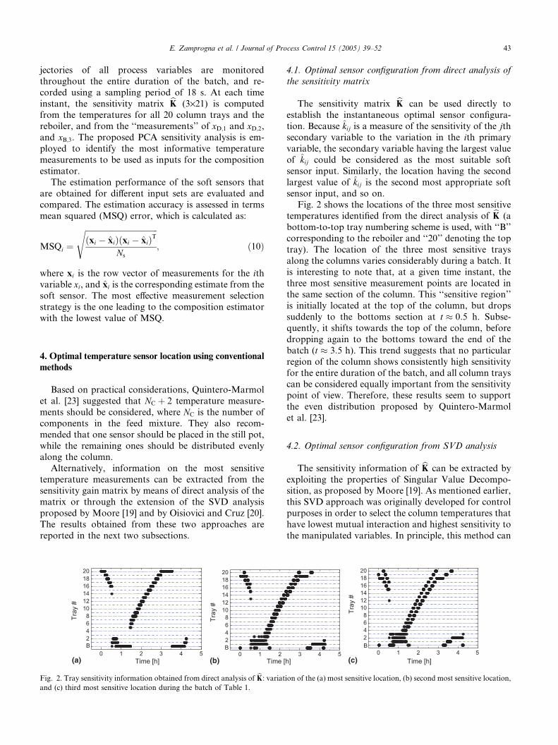
Fig. 2. Tray sensitivity information obtained from direct analysis of bK: variat

and (c) third most sensitive location during the batch of Table 1.

4.1. Optimal sensor configuration from direct analysis of

the sensitivity matrix

The sensitivity matrix bK can be used directly toestablish the instantaneous optimal sensor configura-

tion. Because k̂ij is a measure of the sensitivity of the jthsecondary variable to the variation in the ith primary

variable, the secondary variable having the largest value

of k̂ij could be considered as the most suitable soft

sensor input. Similarly, the location having the second

largest value of k̂ij is the second most appropriate soft

sensor input, and so on.Fig. 2 shows the locations of the three most sensitive

temperatures identified from the direct analysis of bK (a

bottom-to-top tray numbering scheme is used, with ‘‘B’’

corresponding to the reboiler and ‘‘20’’ denoting the top

tray). The location of the three most sensitive trays

along the columns varies considerably during a batch. It

is interesting to note that, at a given time instant, the

three most sensitive measurement points are located inthe same section of the column. This ‘‘sensitive region’’

is initially located at the top of the column, but drops

suddenly to the bottoms section at t � 0:5 h. Subse-

quently, it shifts towards the top of the column, before

dropping again to the bottoms toward the end of the

batch (t � 3:5 h). This trend suggests that no particular

region of the column shows consistently high sensitivity

for the entire duration of the batch, and all column trayscan be considered equally important from the sensitivity

point of view. Therefore, these results seem to support

the even distribution proposed by Quintero-Marmol

et al. [23].

4.2. Optimal sensor configuration from SVD analysis

The sensitivity information of bK can be extracted by

exploiting the properties of Singular Value Decompo-sition, as proposed by Moore [19]. As mentioned earlier,

this SVD approach was originally developed for control

purposes in order to select the column temperatures that

have lowest mutual interaction and highest sensitivity to

the manipulated variables. In principle, this method can

3 4 5h]

0 1 2 3 4 502468

101214161820

B

Tray

#

Time [h](c)

ion of the (a) most sensitive location, (b) second most sensitive location,

0 1 2 3 4 502468

101214161820

B

Time [h]

Tray

#

0 1 2 3 4 502468

101214161820

B

Time [h]

Tray

#

0 1 2 3 4 502468

101214161820

Time [h]

B

Tray

#

(a) (b) (c)

Fig. 3. Tray sensitivity information obtained from SVD analysis of bK: variation of the (a) most sensitive location, (b) second most sensitive location,

and (c) third most sensitive location during the batch.

44 E. Zamprogna et al. / Journal of Process Control 15 (2005) 39–52

be extended to process monitoring. Because of the

properties of the SVD analysis, the application of this

approach to the sensitivity gain matrix bK leads to theidentification of the secondary variables that are least

interacting and most sensitive to the primary variables.

Fig. 3 shows the location of the three most infor-

mative temperatures determined from this approach.

Similarly to the results obtained when using direct

analysis of bK, the location of the most sensitive mea-

surement point (Fig. 3a) changes during the batch, and

all column trays seem to be equally suitable as temper-ature sensor locations. Only the reboiler and the top

column tray could be considered slightly more relevant,

since they correspond to the most sensitive measurement

point for a longer period of time compared to the other

available locations.

The results obtained for the second and third most

sensitive measurements are more difficult to interpret.

As for the second most sensitive measurement location(Fig. 3b), the SVD method suggests that it corresponds

to the reboiler for almost the entire duration of the

process. This result can be explained considering the fact

that one of the estimated variables is the bottoms

composition, and therefore the temperature obtained

from the reboiler is inherently very informative during

the entire operation. Furthermore, sensor interaction is

taken into account in this approach, and biases thechoice of the optimal sensor configuration. Thus, since

the location of the most sensitive temperature usually

0 1 2 3 4 502468

101214161820

B

Time [h]

Tray

#

0 1 202468

101214161820

B

Time

Tray

#

(a) (b)

Fig. 4. Tray sensitivity information obtained from PCA analysis of bK: vari

location, and (c) the third most sensitive location during the batch.

corresponds to one of the column trays, the reboiler is

selected as the second most sensitive point because the

corresponding temperature measurement is likely to bethe least interacting with the first sensor. The latter re-

mark also suggests that the determination of the third

most sensitive measurement location, which is required

to have low interaction with measurements obtained

from both a column tray and the reboiler, could be

difficult. This conjecture is confirmed by the results re-

ported in Fig. 3c, in which it can be observed that the

third most sensitive location tends to change at eachtime instant. From these observations it is possible to

conclude that the SVD analysis of bK suggests placing

one temperature sensor at the top tray and one in the

reboiler. All the other sensors allowed should be evenly

distributed along the column, since all the remaining

possible locations result to be equally important from

the sensitivity point of view.

5. Optimal sensor configuration from PCA sensitivity

analysis

The results obtained from the proposed PCA sensi-

tivity analysis of the sensitivity matrix bK are shown in

Fig. 4. At any given instant, the three most sensitive

trays are located in the same section of the column, asoccurred for the direct analysis of bK. However, in con-

trast to the results obtained from the direct analysis and

3 4 5 [h]

0 1 2 3 4 502468

101214161820

B

Tray

#

Time [h](c)

ation of (a) the most sensitive location, (b) the second most sensitive

0

5

10

15

20

0 50 100 150 200 250 300

Tray

#

Bt = 18 s

CUMPC

Fig. 6. Cumulative sensitivity index CUMPC for each sensor location

for the reference batch.

E. Zamprogna et al. / Journal of Process Control 15 (2005) 39–52 45

from the SVD approach, the optimal sensor locations

identified using the PCA sensitivity analysis are clus-

tered into regions of the column corresponding to its

upper and lower sections only. The trays located in thecentral section of the column are indeed never desig-

nated as ‘‘important’’ measurement locations.

The proposed PCA sensitivity analysis also makes it

possible to determine the number of measurement points

that should be used as inputs to the soft sensor. In fact,

the optimal size of the input measurement set corre-

sponds to the number of the loadings of larger absolute

value. In fact, because each loading represents a measureof the sensitivity of the corresponding temperature

measurement to composition changes, a measurement

should be selected only if its corresponding loading has

a large absolute value, while all measurements whose

loadings are much smaller that the largest one should be

disregarded.

Fig. 5 reports the absolute values of the loadings

calculated during the batch from the largest ðp1Þ to thesmallest ðp21Þ. The value of each loading changes during

the process. However, only the first few loadings (from

p1 to p5) have consistently large values relative to the

others, thus indicating high-sensitivity locations (that

may correspond to different column locations from

sample to sample). Loadings p6 to p15 can be considered

of equally low importance, because their values are

small and their time evolution is very similar, whileloadings p16 to p21 are very small and indicate mea-

surement points that contain very little information

about the primary variables.

0.0 0.1 0.2 0.3 0.4 0.50.00.10.20.30.40.50.60.70.80.91.0

0.0 0.1 0.2 0.3 0.4 0.50.0

0.1

0.2

0.3

0.4

PCA

coef

ficie

nt

p1

p2

p3

p4

p5

p11

p12

p13

p14

p15

Time [h]

PCA

coef

ficie

nt

Fig. 5. Absolute value of the loadings calculated during the batch (for each

cated).

These remarks suggest that five measurement points

could be considered a suitable choice for this case study.According to this analysis, using a larger number of

measurements should not result in any significant

improvement in the accuracy of the composition esti-

mator.

Within the high-sensitivity column regions determined

above, the most suitable locations for sensor placement

can be identified by calculating the cumulative index

CUMPC in Eq. (9). The results in Fig. 6 suggest that thesensitive temperature measurement locations are the re-

boiler (‘‘B’’), and trays # 1, 18, 19, 20.

In the next sections, the effect of the duration of the

sampling period Dt and of measurement noise on the

characterization of the optimal input set via PCA

0.0 0.1 0.2 0.3 0.4 0.50.0

0.1

0.2

0.3

0.4

0.0 0.1 0.2 0.3 0.4 0.50.0

0.1

0.2

0.3

0.4

p6

p7

p8

p9

p10

p16

p17

p18

p19

p20

p21

Time [h]

set of loadings, the average value of the time trajectories is also indi-

46 E. Zamprogna et al. / Journal of Process Control 15 (2005) 39–52

sensitivity analysis are evaluated. The results obtained

using a different analytical formulation for the sensitiv-

ity matrix are also investigated.

5.1. Effect of the sampling interval

In principle, only small sampling intervals should be

used when applying the PCA sensitivity analysis to the

batch distillation process. Small values of Dt are desir-

able because each element of the instantaneous sensi-

tivity gain matrix is approximated by a finite difference

value. Using a large Dt leads to a less accurate estima-tion of K, thus could potentially affect the results of the

PCA sensitivity analysis.

Despite these concerns, Fig. 7 demonstrates that the

results obtained from PCA sensitivity analysis are only

marginally influenced by the length of the sampling

interval. The value of Dt does affect the value of the

cumulative sensitivity index, since the value of CUMPC

for each tray changes with increasing length of Dt.However, the relative importance of each sensor loca-

tion with respect to the other locations remains essen-

tially unchanged.

The robustness of PCA sensitivity analysis to the

sampling interval confirmed by these results is advan-

tageous, as it guarantees that this method provides

consistent results even when a fairly large sampling

interval is used to collect the temperature and compo-sition measurements required to calculate the instanta-

neous sensitivity matrix.

5.2. Effect of measurement noise

Normally distributed noise with zero mean and

standard deviation r was added to the temperatures in

0

5

10

15

20

0 50 100 150 200 250 300CUMPC

Tray

#

B∆t = 18 s

0

5

10

15

20

0 20 40

Tray

#

B

CUM

0

5

10

15

20

0 2 4 6 8 10

CUMPC

Tray

#

B∆ t = 540 s

0

5

10

15

20

0 1 2 3CUM

Tray

#

B

Fig. 7. Effect of the sampling interval Dt on

order to determine whether measurement noise can bias

the results of the PCA sensitivity analysis.

Fig. 8a–c shows the results obtained for the CUMPC

index when the soft sensor inputs are corrupted by noise(from low-level noise, r ¼ 0:1 �C, to high-level noise,

r ¼ 0:5 �C). This measurement noise does affect the

outcome of the PCA sensitivity analysis, because the

profile of CUMPC tends to flatten at increasing noise

levels, thus making it more difficult to rank the available

temperature measurements and identify the most sensi-

tive ones. As confirmed by Fig. 8c, when all tempera-

tures are affected by relatively high-level noise, the PCAsensitivity analysis suggests that the secondary mea-

surements are almost equally sensitive to the product

compositions.

The detrimental effect of measurement noise can

however be easily and effectively counteracted through

appropriate adjustment of the sampling interval. As can

be observed in Fig. 8a, e and i, the CUMPC profile re-

mains practically unaltered when a larger samplinginterval is adopted for larger measurement noise level,

and the PCA sensitivity analysis provides the same

indications obtained when noise free data were used.

Due to the inherent robustness of PCA sensitivity

analysis to the sampling interval, which was shown in

Section 5.1, no disadvantage occurs for the selection of a

larger sampling interval that is appropriate to the level

of the measurement noise.

5.3. Effect of the sensitivity matrix formulation

In Eq. (1), the sensitivity gain has been defined as the

partial derivative of a secondary variable with respect to

a primary variable. As an alternative to this character-

ization, the sensitivity gain could be expressed as the

60 80 100

∆ t = 54 s

PC

0

5

10

15

20

0 5 10 15 20 25 30CUMPC

Tray

#

B∆ t = 180 s

4 5 6PC

∆ t = 900 s 0

5

10

15

20

0.0 0.5 1.0 1.5 2.0 2.5

CUMPC

Tray

#

B∆ t = 1800 s

cumulative sensitivity index CUMPC.

02468

101214161820

0 4 8 12 16 20 24 28 32

a

t = 180 s

Tray

#Tr

ay #

Tray

# = 0.5 °C= 0.3 °Cσ σ σ = 0.1 °C

02468

101214161820

0 4 8 12 16 20 24 28 32

∆∆

∆

∆

t = 180 s

b

02468

101214161820

0 2 4 6 8 10

d

t = 540 s02468

101214161820

0 1 2 3 4 5 6 7 8 9 10

t = 540 s

f

02468

101214161820

0 1 2 3 4 5 6 7

g

∆

∆

∆

∆

∆

t = 900 s 02468

101214161820

0 1 2 3 4 5 6 7

t = 900 s

h

02468

101214161820

0 1 2 3 4 5 6 7

t = 900 s

i

CUMPC CUMPC CUMPC

02468

101214161820

0 4 8 12 16 20 24 28 32

t = 180 s

c

02468

101214161820

0 2 4 6 8 10

t = 540 s

e

Fig. 8. Effect of measurement noise on the cumulative sensitivity index CUMPC.

E. Zamprogna et al. / Journal of Process Control 15 (2005) 39–52 47

partial derivative of a primary variable with respect a

secondary variable. In this case, the resulting sensitivity

matrix is:

Kinv ¼

ox1oT1

� � � ox1oTj

� � � ox1oTn

..

. ... ..

.

oxioT1

� � � oxioTj

� � � oxioTn

..

. ... ..

.

oxmoT1

� � � oxmoTj

� � � oxmoTn

266666664

377777775; ð11Þ

which can be approximated at each time instant t as:

0 1 2 3 4 502468

101214161820

B

Tray

#

Time [h]0 1 2

02468

101214161820

B

Tray

#

Time(a) (b)

Fig. 9. Tray sensitivity information obtained from PCA analysis of bKinv: v

location, and (c) third most sensitive location during the batch.

bKinvðtÞ ¼

Dx1DT1

� � � Dx1DTj

� � � Dx1DTn

..

. ... ..

.

DxiDT1

� � � DxiDTj

� � � DxiDTn

..

. ... ..

.

DxmDT1

� � � DxmDTj

� � � DxmDTn

2666666664

3777777775: ð12Þ

We will refer to bKinv as the ‘‘inverse’’ sensitivity matrix,to distinguish it from the ‘‘direct’’ sensitivity matrix bKðtÞin Eq. (4).

As shown in Fig. 9, the results obtained from the

application of the PCA analysis to the inverse sensitivity

3 4 5 [h]

0 1 2 3 4 502468

101214161820

B

Tray

#

Time [h](c)

ariation of the (a) most sensitive location, (b) second most sensitive

0

5

10

15

20

0 50 100 150 200 250 300

∆t = 18 s

Tray

#

B

CUMPC

0

5

10

15

20

0 20 40 60 80 100

Tray

#

B ∆t = 54 s

CUMPC

0

5

10

15

20

0 5 10 15 20 25 30

Tray

#

B ∆t = 180 s

CUMPC

0

5

10

15

20

0 2 4 6 8 10

Tray

#

B Dt = 540 s

CUMPC

0

5

10

15

20

0 1 2 3 4 5 6

Tray

#

B ∆t = 900 s

CUMPC

0

5

10

15

20

0.0 0.5 1.0 1.5 2.0 2.5 3.0

Tray

#

B ∆t = 1800 s

CUMPC

Fig. 10. Effect of the sampling interval Dt on the cumulative sensitivity index CUMPC (PCA analysis of bKinv).

48 E. Zamprogna et al. / Journal of Process Control 15 (2005) 39–52

matrix for the benchmark batch distillation column are

clearly different from the results obtained previouslywhen the direct gain is employed. Thus, a different

characterization of the column sensitivity affects the

information content of the sensitivity matrix.

The location of the three most informative measure-

ment points varies during the operation. In general, the

optimal locations correspond to the top trays at the

beginning of the operation, shift down to the column

during the first part of the batch process, and then reversethis trend reaching to the top trays again. It is interesting

to note that in this case the reboiler and the bottom

column trays are never considered as sensitive measure-

ment points, despite the fact that one of the primary

variables is the composition of the bottom product.

As shown in Fig. 10, the sensitivity index CUMPC

(Dt ¼ 18 s) indicates that the overall optimal sensor

locations correspond to trays # 7, 8, 9, 19, 20, when fivemeasurements points are allocated. This result however

is affected by the sampling interval used to collect the

data. Also, because the value of the cumulative sensi-

tivity index CUMPCi for the ith location decreases with

increasing Dt, the variation of the sampling period alters

the relative importance of the available temperature

measurements. As a result, the characterization of the

optimal temperature set changes at different values ofDt. This is a major disadvantage, and it suggests that this

sensitivity gain formulation is not appropriate.

6. Development of a composition estimator using alterna-

tive sensor configurations

In order to assess which measurement selectionstrategy is the most effective one among the ones con-

sidered so far, composition soft sensors have been

developed using temperature measurements from theoptimal sensor configurations identified considering

different approaches of sensitivity analysis. In particu-

lar, linear PLS, nonlinear PLS, and ANN models have

been evaluated. For the PLS estimators, three latent

variables were retained in the regression models, this

number having been determined using cross-validation.

As shown by Zamprogna et al. [28], this approach

inherently rejects the effect of noise in the temperaturemeasurements, because random noise is typically asso-

ciated with the higher-order latent variables, and is

therefore eliminated when the original data are pro-

jected onto a lower dimensional space. Therefore,

measurement noise will not be considered in the fol-

lowing example, because it has a negligible effect on the

accuracy of composition estimations. Note however

that noise may impact (even markedly) the performanceof the ANN estimator.

To allow for a wider comparison, several alternative

randomly chosen configurations were also considered.

The results obtained for four of these supplementary

configurations (AC1, AC3, AC4, and AC5) have been

reported, as a representation of the estimation perfor-

mances that are typically achieved when no specific

measurement selection strategy is adopted. All theconfigurations considered are collected in Table 2.

Temperature measurements from each selected con-

figuration are used by the soft sensors to estimate the

light and intermediate component mole fraction in the

distillate stream and the heavy component mole fraction

in the reboiler during the entire duration of the batch.

The most effective measurement selection approach is

the one that leads to the soft sensor that has the lowestestimation error MSQ for the validation data. The

Table 2

Summary of the optimal sensor locations obtained using different measurement selection approaches

Measurement selection approach Symbol Most sensitive locations (tray #)

Even distribution [23] ED B 05 10 15 20

Direct sensitivity analysis DA�ED B 05 10 15 20

SVD sensitivity analysis SVD�ED B 05 10 15 20

PCA sensitivity analysis (optimal location) OL B 01 18 19 20

Alternative configuration #1 AC1 B 01 02 03 20

Alternative configuration #2 AC2 03 12 15 16 19

Alternative configuration #3 AC3 01 07 08 18 19

Alternative configuration #4 AC4 B 02 04 05 12

PCA sensitivity analysis using inverse gain matrix AC5 07 08 09 19 20

E. Zamprogna et al. / Journal of Process Control 15 (2005) 39–52 49

operating conditions for the validation data are reported

in Table 3.

Fig. 11 represents the values of the prediction error

MSQ calculated for the validation data for the PLS and

ANN soft sensors using input data from all the con-

sidered measurement configurations. The most accurate

estimation performance is obtained by using the same

measurement set for all the soft sensors. The best con-figuration is OL of Table 2, because it has the minimum

Table 3

Operating conditions for the validation data

Mixture relative volatility, a1=a2=a3 9/3/1

Feed composition, xF;1=xF;2=xF;3 0.33/0.50/0.17

Feed charge, F 300 mol

Vapor boilup rate, V 70 mol/h

Distillate withdrawal rate, D 40.54 mol/h

Nominal composition setpoint, xspP1=xspP2=x

spP3 0.95/0.95/0.95

0

5

10

15

20

25

305075

100

TotalxD,2xD,1

xB,3

Linear PLS

MSQ

x 1

03

3

2

0

5

10

15

20

25

305075

100

EDOLAC1

AC2

AC3

AC4

AC5

xD,xD,1

MSQ

x 1

03

Fig. 11. Validation error MSQ for a linear PLS, a nonlinear PLS, and an A

inputs.

value of the total MSQ for both the PLS soft sensors

and the ANN soft sensor.

A very large estimation error in the distillate com-

positions occurs when only temperature measurements

in the lower section of the column are used (configura-

tion AC4). Configuration AC2 usually leads to models

having relatively large values of MSQ. These results

suggest that (as is intuitively expected) it is not desirableto exclude the temperature measurements located in the

reboiler from the optimal input set (as in configurations

AC2, AC3 and AC5). In general, reduced estimation

performance results when using input data from con-

figuration AC3, which includes temperature measure-

ments located in the central section of the column. This

observation confirms that these locations are poorly

representative of the output variables, as noted in Sec-tion 5. Poor estimation performance is observed also

when using configuration AC5. This fact suggests that

0

5

10

15

20

25

305075

100

TotalxD,2xD,1xB,3

Nonlinear PLS

MSQ

x 1

0

TotalxB,3

ANN

NN soft sensors when using five temperature measurements as model

50 E. Zamprogna et al. / Journal of Process Control 15 (2005) 39–52

that the indications obtained by performing the PCA

sensitivity analysis for the inverse gain matrix are in this

case misleading.

Fig. 11 also shows that all the soft sensors usingconfiguration OL provide the overall most accurate

0.0 0.5 1.0 1.5 2.0 2.5

0.0

0.2

0.4

0.6

0.8

1.0

0.0 0.5 1.0 1.5 2.0 2.5

0.0

0.2

0.4

0.6

0.8

1.0

0.0 0.5 1.0 1.5 2.0 2.5

0.0

0.2

0.4

0.6

0.8

1.0

Actual Linear PLS, OL

xB,3

Time [h]

xD,1

xD,2

(a)

Fig. 12. Validation data: comparison between the product compositions and

measurements from configuration OL (a) and configuration ED (b).

1 2 3 4 5 6 7 8 9 10 110

2

4

6

8

10

211612

xD,1

MSQ

x 1

03

1 2 3 4 5 6 7 8 9 10 110

2

4

6

8

10

16 2112

xB,3

Number of measurements

MSQ

x10

3

Fig. 13. MSQ validation error for linear PLS soft sensors using configu

composition estimation, and are almost equally accu-

rate. The linear PLS soft sensor can be considered to be

the most suitable one for this case study, because it

shows the lowest MSQ error and has a simpler structurecompared to the nonlinear PLS or ANN estimators.

0.0 0.5 1.0 1.5 2.0 2.50.0

0.2

0.4

0.6

0.8

1.0

1.2

0.0 0.5 1.0 1.5 2.0 2.5

0.0

0.2

0.4

0.6

0.8

1.0

0.0 0.5 1.0 1.5 2.0 2.5

0.0

0.2

0.4

0.6

0.8

1.0

Actual Linea r P LS, ED

Time [h]

(b)

their estimates provided by a linear PLS soft sensor using temperature

1 2 3 4 5 6 7 8 9 10 110

2

4

6

8

10

Number of measurements

211612

xD,2

1 2 3 4 5 6 7 8 9 10 1102468

1012141618202224

211612

Total

ration OL with different numbers of temperature measurements.

E. Zamprogna et al. / Journal of Process Control 15 (2005) 39–52 51

This topic has been further discussed by Zamprogna

et al. [28].

Fig. 12 compares the actual value of the product

compositions and their estimates calculated by the linearPLS model for the validation data. This figure provides

further confirmation that configuration OL provides

good estimates of the composition profiles.

In particular, the estimation accuracy is higher than

what can be obtained when using the configuration

usually suggested (configuration ED) [23], where the

temperature sensors are evenly distributed along the

column.

6.1. Effect of the number of temperature measurements

The PCA sensitivity analysis carried out in Section 5

suggests a priori that the optimal number of tempera-ture measurements for the regression model is five. In

order to verify this result, linear PLS estimators have

been developed using configurations having a different

number of measurements.

The temperature measurements for each configura-

tion have been selected according to the location rank-

ing suggested by the PCA sensitivity analysis. The

estimation error calculated for the linear PLS modelsobtained are represented in the form of bar plots in

Fig. 13.

For the estimation of xD;1 and xD;2 in Fig. 13, the

value of MSQ depends quite markedly upon the number

of temperatures incorporated in the optimal set. The

minimum MSQ is indeed achieved by a soft sensor using

the configuration OL with five measurements, as indi-

cated by the PCA sensitivity analysis (a soft sensor usingfour input measurements provides almost the same

accuracy, however). The number of measurements in-

cluded in configuration OL affects only marginally the

accuracy of estimation xB;3; the MSQ index for this

primary variable shows however a minimum when three

temperature measurements are considered.

7. Conclusions

A novel methodology has been proposed in order to

identify the most suitable number and locations of

temperature measurements to be used as soft sensor

inputs for estimating composition profiles in a batch

distillation column. The proposed approach is based on:

(i) the characterization of the instantaneous sensitivityof each secondary variable to the primary variables, and

(ii) on the identification of the most sensitive secondary

variables from this sensitivity matrix by exploiting the

properties of the PCA transformation.

The simulation results have shown that the proposed

approach can effectively help to select the most infor-

mative secondary process variables, leading to a soft

sensor with good estimation performance. It has also

been shown that the length of the sampling interval af-

fects the results obtained from the PCA sensitivity

analysis only marginally. Even though the presence ofmeasurement noise can make it more difficult to rank

the available temperature measurements and to identify

the most sensitive ones through the PCA sensitivity

analysis, it was shown that the detrimental effects of

measurement noise can be counteracted through ap-

propriate adjustment of the sampling interval.

The proposed methodology can be easily extended to

other batch processes, and to distributed parametersystems. In this regard, interesting results are being

obtained for the optimal selection of input measure-

ments in tubular reactors, and the results will be re-

ported elsewhere.

Acknowledgements

This research was carried out in the framework of the

MIUR-PRIN 2002 project ‘‘Operability and controlla-

bility of middle-vessel distillation columns’’ (ref. no.

2002095147_002).

References

[1] M. Barolo, F. Berto, Composition control in batch distillation:

binary and multicomponent mixtures, Ind. Eng. Chem. Res. 37

(1998) 4689–4698.

[2] M. Barolo, A. Pistillo, A. Trotta, Issues in the development of a

composition estimator for a middle vessel batch column, in: L.T.

Biegler, A. Brambilla, C. Scali (Eds.), Advanced Control of

Chemical Processes 2000––IFAC ADCHEM 2000, Elsevier,

Oxford, UK, 2000, pp. 923–928.

[3] B.W. Bequette, T.F. Edgar, Non-interacting control system design

methods in distillation, Comp. Chem. Eng. 13 (1989) 641–

650.

[4] B.W. Bequette, T.F. Edgar, Selection of process measurements in

distillation column control to minimize multivariable interactions,

AIChE Annual Meeting, San Francisco, USA, 1984.

[5] C. Brosilow, B. Joseph, Techniques of Model Based Control,

Prentice Hall, New York, USA, 2002.

[6] I. Chien, B.A. Ogunnaike, Modeling and control of a tempera-

ture-based high-purity distillation column, Chem. Eng. Commun.

158 (1997) 71–105.

[7] P. Geladi, B.R. Kowalski, Partial least-squares regression: a

tutorial, Anal. Chim. Acta 185 (1986) 1–17.

[8] C. Georgakis, D.H. Kindt, M. Kasotaki, Extensive variable

control structures for binary distillation columns, AIChE Annual

Meeting, San Francisco, USA, 1984.

[9] S.S. Haykin, Neural Networks: A Comprehensive Foundation,

second ed., Prentice Hall, New York, USA, 1999.

[10] J.E. Jackson, A User’s Guide to Principal Components, John

Wiley & Sons, New York, USA, 1991.

[11] B. Joseph, C.B. Brosilow, Inferential control of processes. Part I:

steady state analysis and design, AIChE J. 24 (1978) 485–

492.

[12] R.E. Kalman, A new approach to linear filtering and prediction

problems, Trans. ASME, J. Basic Eng. 82 (1960) 35–45.

52 E. Zamprogna et al. / Journal of Process Control 15 (2005) 39–52

[13] M. Kano, K. Miyazaki, S. Hasebe, I. Hashimoto, Inferential

control system of distillation compositions using dynamic partial

least squares regression, J. Process Control 10 (2000) 157–

166.

[14] T. Kourti, J.F. MacGregor, Tutorial: Process analysis, monitoring

and diagnosis, using multivariate regression methods, Chemom.

Intell. Lab. Syst. 28 (1995) 3–21.

[15] H. Leegwater, Industrial experience with double quality control,

in: W.L. Luyben (Ed.), Practical Distillation Control, Van

Nostrand Reinhold, New York, USA, 1992.

[16] D.C. Luenberger, Observing the state of a system, IEEE Trans.

Military Electron. MIL-8 (1964) 74–80.

[17] W.L. Luyben, Multicomponent batch distillation.1. Ternary

systems with slop recycle, Ind. Chem. Eng. Res. 27 (1991) 642–

657.

[18] T. Mejdell, S. Skogestad, Estimation of distillation compositions

from multiple temperature measurements using partial-least-

squares regression, Ind. Eng. Chem. Res. 30 (1991) 2543–

2555.

[19] C.F. Moore, Selection of controlled and manipulated variables,

in: W.L. Luyben (Ed.), Practical Distillation Control, Van

Nostrand Reinold, New York, USA, 1992.

[20] R.M. Oisiovici, S.L. Cruz, Sensor location and noise reduction in

high-purity batch distillation control loops, Braz. J. Chem. Eng.

17 (2000) 671–683.

[21] R. Osiovici, S.L. Cruz, Inferential control of high-purity multi-

component batch distillation columns using an extended Kalman

filter, Ind. Eng. Chem. Res. 40 (2001) 2628–2639.

[22] S.J. Qin, Neural network for intelligent sensors and control––

practical issues and some solutions, in: O. Omidvar, D.L. Elliott

(Eds.), Neural Systems for Control, Academic Press, New York,

USA, 1997.

[23] E. Quintero-Marmol, W.L. Luyben, C. Georgakis, Application of

an extended Luenberger observer to the control of multicompo-

nent batch distillation, Ind. Chem. Eng. Res. 30 (1991) 1870–1880.

[24] D.E. Seborg, T.F. Edgar, D.A. Mellichamp, Process Dynamics

and Control, second ed., John Wiley & Sons, New York, USA,

2004.

[25] T.L. Tolliver, L.C. McCune, Distillation control design based on

steady state simulation, ISA Trans. 17 (1978) 3–10.

[26] E. Zamprogna, M. Barolo, D.E. Seborg, Composition estimations

in a middle-vessel batch distillation column using artificial neural

networks, Chem. Eng. Res. Des. 79 (2001) 689–696.

[27] E. Zamprogna, Development of virtual sensors for batch distil-

lation monitoring and control using multivariate regression

techniques, Ph.D. Dissertation, Department of Chemical Engi-

neering Principles and Practice, University of Padova, Italy, 2001.

[28] E. Zamprogna, M. Barolo, D.E. Seborg, Estimating product

composition profiles in batch distillation via partial-least-squares

regression, Control Eng. Practice 12 (2004) 917–929.