USDOT Region V Regional University Transportation Center Final Report IL IN WI MN MI OH NEXTRANS Project No. 019FY02 OPTIMAL SIGNAL TIMING DESIGN FOR URBAN STREET NETWORKS UNDER USER EQUILIBRIUM BASED TRAFFIC CONDITIONS By Dr. Zongzhi Li Associate Professor Illinois Institute of Technology [email protected]and Dr. Lili Du Assistant Professor Illinois Institute of Technology [email protected]and Yi Liu, Ph.D. Graduate Research Assistant Illinois Institute of Technology [email protected]
Transcript
USDOT Region V Regional University Transportation Center Final Report
IL IN
WI
MN
MI
OH
NEXTRANS Project No. 019FY02
OPTIMAL SIGNAL TIMING DESIGN FOR URBAN STREET NETWORKS UNDER USER EQUILIBRIUM BASED TRAFFIC CONDITIONS
Funding for this research was provided by the NEXTRANS Center, Purdue University under Grant No. DTRT12-G-UTC05 of the U.S. Department of Transportation, Office of the Assistant Secretary for Research and Technology (OST-R), University Transportation Centers Program. The contents of this report reflect the views of the authors, who are responsible for the facts and the accuracy of the information presented herein. This document is disseminated under the sponsorship of the Department of Transportation, University Transportation Centers Program, in the interest of information exchange. The U.S. Government assumes no liability for the contents or use thereof.
USDOT Region V Regional University Transportation Center Final Report
TECHNICAL SUMMARY
NEXTRANS Project No 019PY01Technical Summary - Page 1
IL IN
WI
MN
MI
OH
NEXTRANS Project No. 019FY02 Final Report, September 20, 2016
Title OPTIMAL SIGNAL TIMING DESIGN FOR URBAN STREET NETWORKS UNDER USER EQUILIBRIUM BASED TRAFFIC CONDITIONS
Introduction In the ever-growing travel demand, traffic congestion on freeways and expressways recurs more frequently at a higher number of locations and for longer durations with added severity. This becomes especially true in large metropolitan areas. Particular to the urban areas, excessive crowdedness caused by inefficient traffic control also results in urban street networks operating in near or over-saturated conditions, leading to unpleasant travel experience due to long delays at intersections. As a consequence, the recurrent traffic congestion on roadway segments and vehicle delays at intersections inevitably compromise energy efficiency, traffic mobility improvement, safety enhancement, and environmental impacts mitigation. All too often, neither restraining travel demand nor expanding system capacity is desirable and practical. Conversely, effectively utilizing the capacity of the existing transportation system has been increasingly thought of as the solution to congestion relief. With respect to the urban street networks, developing effective means for urban intersection signal optimization becomes essential to reduce intersection delays.
Traffic signal control is used to determine who has the right of way at a signalized intersection and also able to control the flow patterns of traffic through the intersection. Early contributions in this area were mainly focusing on optimize signal settings, such as the total cycle time and the green splits, for a single isolated intersection (Webster, 1958). Such approaches could surely reduce the vehicle delays at single intersection, and be stretched to the entire network by applying the techniques to every intersection in the network. However, coordination between traffic signals in close proximity and their mutual effect on the network traffic assignment are not considered.
Conventional fixed time signal plan optimization strategies, as mentioned earlier, use historical traffic data and assume that traffic flows will remains unchanged after the implementation of new signal plans. Traffic flows were assumed to be given and invariable, but, in fact, when signal timings change, travel times for certain or all travel routes will be different, which definitely makes drivers in the network to adjust their choice of travel paths to destinations, and result in changes of traffic flows in the network. Then, new optimal signal settings are always required if they were treated independently with traffic flows. In an attempt to maintain the interdependency between traffic assignment and signal control, it
NEXTRANS Project No 019PY01Technical Summary - Page 2
was put forward that impacts of signal settings on the traffic flows should be considered by combining traffic control and route choice (Allsop 1974).
There are two different ways to solve this problem: the iterative optimization and assignment procedure and the combined optimization and assignment model. This study falls in the latter approach.
The iterative optimization and assignment procedure is to alternatively update signal timings with fixed traffic flows and solve the traffic equilibrium problem for the new signal settings until a mutually consistent (MC) solution is gained. This approach has the advantage that it actually solves the traffic assignment problem and signal timing optimization problem separately, using traditional traffic assignment and signal timing optimization techniques. Also, it can be applied on large networks much more easily compared to combined optimization and assignment model approach. But it has been pointed out theoretically and empirically by Dickson (1981) that this approach cannot guarantee to converge even to a local optimum, and also may lead to an increase in total delay over the network rather than a decrease. And this the main reason that leads this study to the combined signal timing optimization and traffic assignment model approach.
The combined signal timing optimization and traffic assignment model seeks optimal signal settings such that one or more system performance measures like the total travel time or average delay are minimized, while the driver’s routing is simultaneously ascribed by a traffic equilibrium model. This combined problem is an instance of the network design problem (NDP), which is concerned with improving an existing network, meanwhile considering the user’s response to the change. A bi-level structure can be employed to model this combined problem in which signal timing optimization is regarded as the upper level problem while user equilibrium traffic assignment is regarded as the lower level problem. Two major difficulties that involved in this approach need to be mentioned. One of them, which is with respect to problem solving, is that the problem is generally hard to solve because of the high complexity which comes from the non-convexity of objective functions and constraints at both level. Most previous studies on this approach focused on seeking an efficient algorithm, which was capable of finding a local optima or near-global optima of the signal setting variables in the upper level and simultaneously finding the user-decided flow pattern for the lower level. Another major difficulty of the combined problem approach, which is much less extensively studied, is the integration of time delay at signalized intersection to the bi-level optimization model. Some of the existing works, which are analytical-based, use an oversimplified assumptions of the traffic signal control system, and apply it to a small sample network. While other methods, most recent works, which were simulation-based, require an existing simulation model of the network such as TRANSYT to evaluate the performance of the system with different signal settings, and demands extensive data and work to build such simulation model before optimization. It is a costly and time consuming work when dealing with real world problems, comparing with other methods that uses analytical mathematical expression to formulate the system, and is generally not possible for states and agencies that do not maintain rich data on travel demand, facility preservation, traffic operations, data processing and preparation capacity, and have high performance computing facilities. The above-mentioned shortcomings all constraint potential employment of the methods for a real world network.
NEXTRANS Project No 019PY01Technical Summary - Page 3
The above mentioned shortcomings motivate the author to address the combined optimization and assignment problem analytically as a rigorous Mathematical Problem with Equilibrium Constraints (MPEC) general assumptions and formulations, meanwhile, model and evaluate traffic signal controlled systems accurately, and also makes it well applicable to real world problems. Delay calculation and static user equilibrium will all be formulated as Variational Inequality constraints which allow the state-of-the-art MPEC solver, GAMS/NLPEC, to be employed for solving the problem for a local optimal effectively and efficiently.
Moreover, as one variable of the signal settings that can be adjusted to potentially improve the effectiveness of traffic signal plans, signal phasing design has received little attention from researchers. In bandwidth maximization approach, it was indicated that left-turn sequence had significant effectiveness. Tian et al. (2008) indicated that lead-lag phasing showed clear advantages over other phasing sequence in maximizing progression bandwidth. Meanwhile, various signal phasing designs provide different behaviors in terms of delays for different approach. For instance, comparing to lag left-turn phasing, lead left-turn phasing, which has a protected left-turn phase prior to through phase, can reduce the average signal control delays for corresponding left-turn traffic by reducing the continuous queuing time, which, as a consequence, reduces the maximum queue length. While, this also results in more continuous queuing time assigned to the opposing through traffic. Main reason that limits adding signal phasing to the delay-based signal optimization programs is the computational infeasibility that appeared (Cohen and Mekemson, 1985). Based on the MPEC model proposed earlier, the author attempts to develop an enhanced model that takes different signal phasing design into account. To model the selection of signal phasing designs, integer variables will be required in the enhanced model. However, GAMS/NLPEC solver has its limitation when dealing with integer programing, and it was built to solve problems with continuous variable only. Therefore, different solution algorithms will be proposed and attempt to solve this enhanced model.
In general, the author introduces a new methodology in this study that addresses the combined signal timing optimization and traffic assignment problem analytically with general assumptions and formulations, which models and evaluates traffic signal controlled systems accurately, and is also well applicable to real world problems. In the proposed method, urban network traffic signal timing optimization and traffic flow equilibrium problem are considered as a bi-level optimization problem. A basic model is proposed firstly, which attempt to minimize system total travel time by optimizing signal green splits. HCM 2010 delay method, which is one of the most up-to-date time-dependent stochastic delay models, is employed as intersection delay estimation method in the model, and is formulated as Variational Inequality constraints, what allow the state-of-the-art MPEC solver, GAMS/NLPEC, to be employed for solving the problem for a local optimal effectively and efficiently. A small sample network and a real world network in the densely populated City of Chicago area are used to test the capability of the model and the applicability to real world case in urban area.
Furthermore, in order to import more reality to the basic model and also consider the potential system benefit that comes from different signal phasing design, an enhanced model is developed based on the basic model by employing integer and binary variables. Then, the enhanced model belongs to a new
NEXTRANS Project No 019PY01Technical Summary - Page 4
class of challenging optimization problems, namely Mixed-Integer Nonlinear Programming (MINLP) with Complementarity Constraints. Formulating the problem with binary variables allows for the selection of proper phasing design. Heuristic solution algorithms are proposed and tested in a small sample network.
Findings In this study, intersection control delay calculation method introduced in HCM 2010 has been employed in a combined optimization problem for area traffic signal control and network traffic assignment, and formulated as Variational Inequality (VI) constraints in the basic MPEC model. It allows the proposed method to accurately model and estimate the intersection control delay of various type of movements in real world scenarios such as those with multiple green phases and multiple control methods (protected, permitted, or mixed) without the use of simulation-based traffic model. The combined problem was formulated as mathematical programming with equilibrium constraints (MPEC) and solved by using GAMS/NLPEC solver which reformulates and solves the MPEC problem as standard nonlinear programming (NLP).
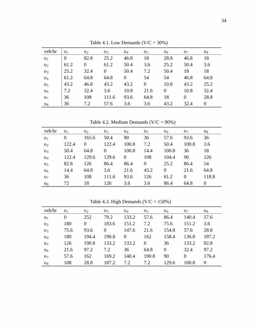
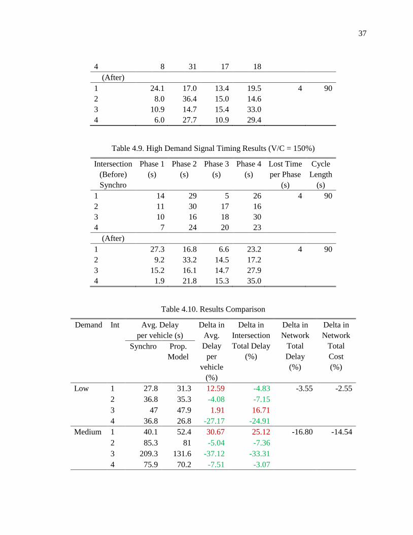
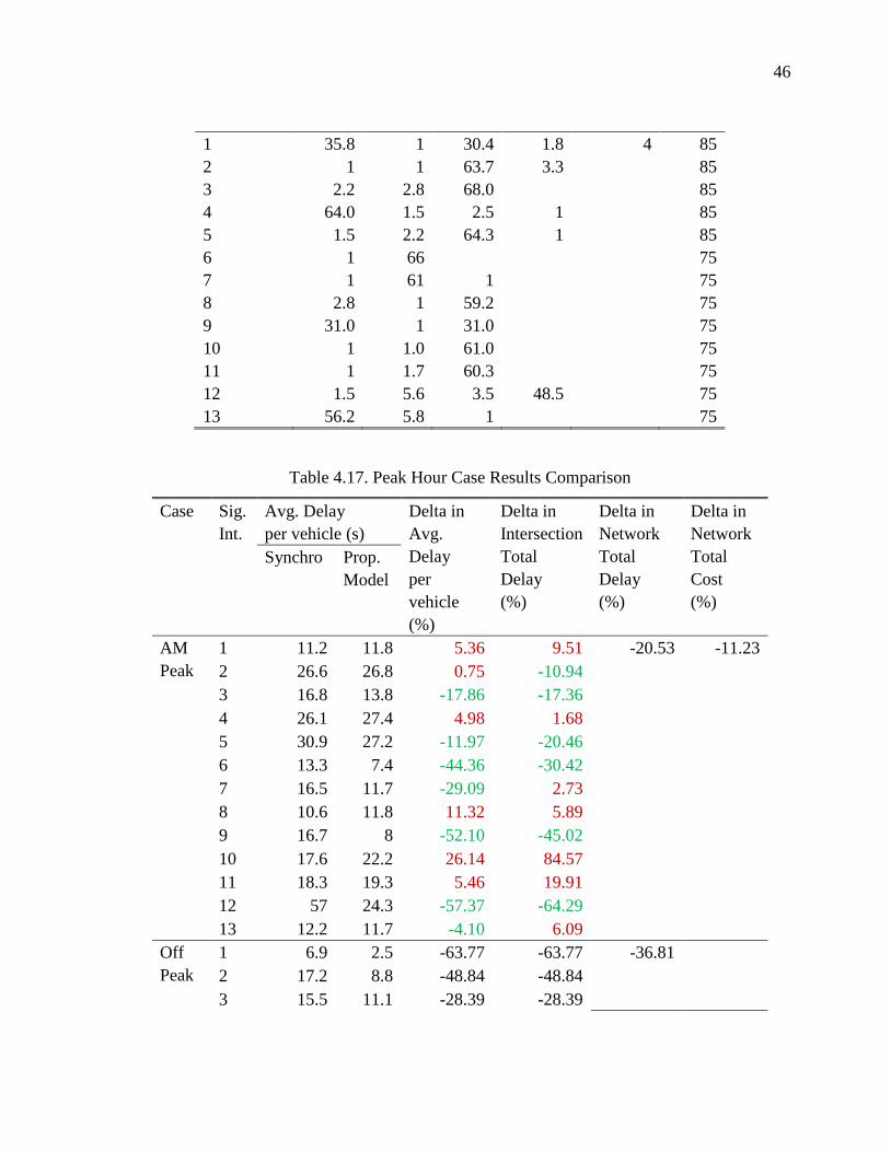
The basic MPEC model was applied on an experimental 4-intersection network and a real world problem with 13 signalized intersection in the City of Chicago urban area. Different phasing plans were adopted in the experimental network, and three traffic loads were tested as different cases from low traffic demand condition case (with intersection V/C around 30%) to high traffic demand condition case (with intersection V/C around 150%). Comparing the optimization results of the proposed model with the optimization results by using Synchro with the same initial traffic assignment, improvements in both total intersection control delay and total travel cost were observed in all three cases, and they varied significantly. Small improvement, 2.55% in total travel time reduction, was obtained in the low demand case, and large improvement, 14.54% in total travel time reduction, was showed in the medium demand case which has near capacity traffic loads at signalized intersections. After the optimization, drivers tended to switch their route from intersections with protected only left-turn phasing to intersections with protected-permitted left-turn phasing and split phasing, where more left turn traffic would better utilize the intersection capacity. Comparing with the protected left-turn only phasing, protected-permitted left-turn phasing and split phasing had relatively more capacity without occupying the green time for other phases.
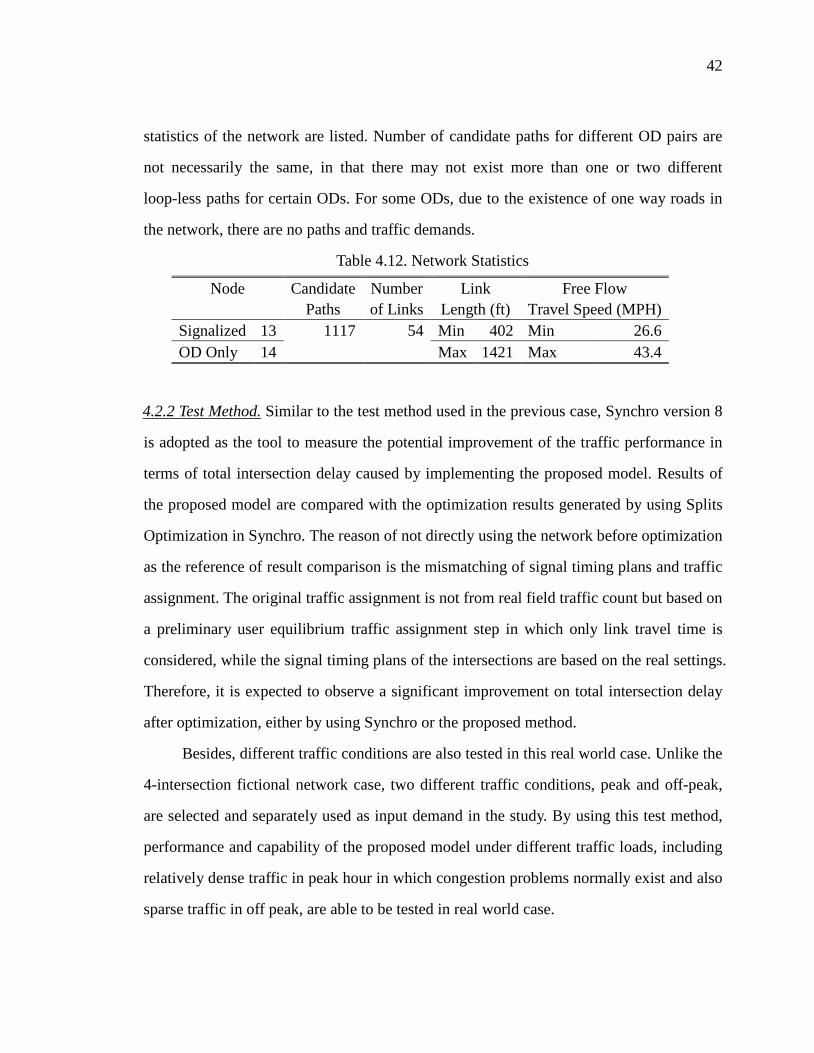
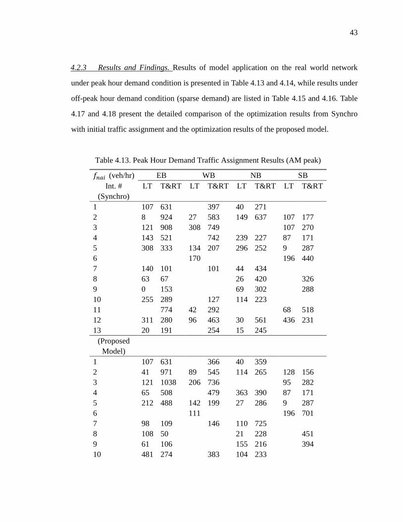
For the real world problem, named as network two, two different OD demands generated by Chicago TRANSIMS microscopic traffic simulation model were tested. In the case with AM peak traffic demand, which is roughly 30% V/C, 11.23% total travel time reduction was obtained from the proposed method when compared with Synchro optimization result, and almost all of the travel time reduction was contributed by reduction in intersection control, 20.53%, in that network total link travel time remained basically the same with 0.28% increase. Under similar demand condition, 30% V/C ratio, the basic MPEC model tend to be more applicable and beneficial in larger network than small network with limited paths and intersections. Besides, it was also observed that changes in the traffic routing was the main reason and power that caused the improvement in system performance, and is also the major difference between Synchro and the basic MPEC model proposed in this study. However, in the case with off peak traffic demand, although the significance of result comparison was lost because of the bad optimization
NEXTRANS Project No 019PY01Technical Summary - Page 5
results from Synchro, it was still able to present the capability of the proposed model when dealing with extremely low demand situation.
Furthermore, in order to import more reality to the basic model and consider the potential system benefit that comes from different signal phasing designs, an enhanced model is developed based on the basic MPEC model by employing binary variables to make selection of optimal signal phasing plans from pre-defined candidates. The enhanced model belongs to a new class of challenging optimization problems, namely Mixed-Integer Nonlinear Programming (MINLP) with Complementarity Constraints. Formulating the problem with binary variables allows for the selection of proper phasing design, however, also increase the difficulty to solve the problem. As preliminary solution attempts, two heuristic solution algorithms, GA method and EA method, are proposed.
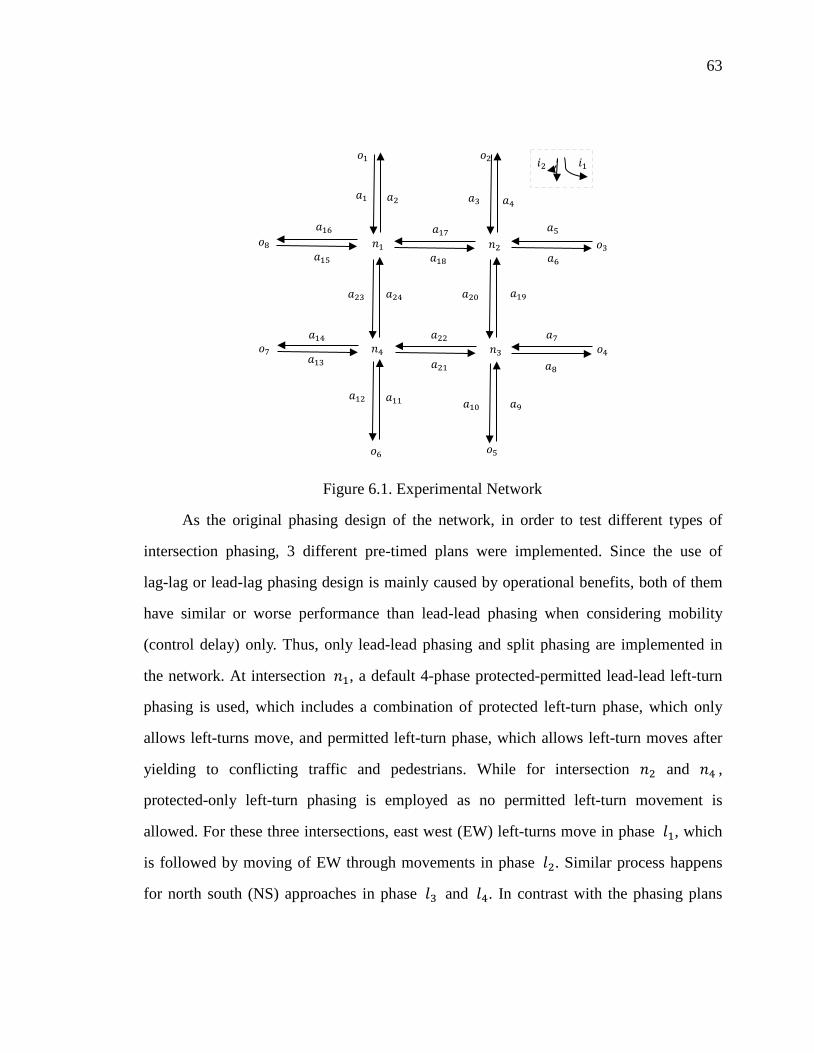
Both GA and EA solution method were implemented on the test network to verify the feasibility of the solution methods. In the network, one lead-lead left turn phasing and one split phasing designs were prepared as candidates for intersection 2 and 3, respectively. In total, 4 different combination of phasing plans were available in the problem.
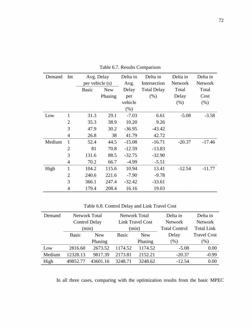
Among two preliminary solution methods, GA failed to provide valid nor optimal solution within valid running period. While EA method, which highly relies on the basic MPEC model, provided optimal results when keeping original phasing at intersection 2 unchanged and replacing the split phasing at intersection 3 with normal lead-lead phasing. Comparing with the optimization results of the original phasing plans, 3.58%, 17.46%, and 11.77% reduction in network total cost were observed under low, medium, and high traffic demand conditions, respectively. Similar to previous cases, all reduction came from the improvement at signalized intersections, particularly, from intersection 3. The results strongly supported our assumption that adding phasing design as a variable in the model would further generate potential improvement in the system.
Recommendations The application of the basic MPEC model, along with the solution method, does not require extensive data collection, preparation, and computational efforts as compared to the methods that rely on simulation-based traffic models to evaluate the performance of traffic signals. This gives it potentially greater applications to agencies that do not maintain rich data on travel demand, facility preservation, traffic operations, data processing and preparation capacity, and high performance computing facilities. However, current solution method relies on a good initial point to obtain an acceptable optimization result, and it would be useful to develop a better method to find a good initial point or initial feasible solution as future work.
For the enhanced model, an efficient solution algorithm is still under development. Both of the proposed preliminary solution methods have their limitations and required more research. Looking for an alternative of SUE, which allows more tolerance when locating feasible solutions, could be a future research direction for the GA method approach. Meanwhile, for EA method approach, a reduction method, which is able to effectively reduce the size of candidate phasing design combinations without losing solution optimality, are also needed to improve method’s efficiency.
NEXTRANS Project No 019PY01Technical Summary - Page 6
Contacts For more information:
Dr. Zongzhi Li, Ph.D., Associate Professor Illinois Institute of Technology 3201 South Dearborn Street, AM Hall, Room 211 Chicago, IL 60616 Phone: (312) 567-3556 Fax: (312) 567-3519 Email: [email protected]
NEXTRANS Center Purdue University - Discovery Park 3000 Kent Ave. West Lafayette, IN 47906 Phone: (765) 496-9724 Email: [email protected] www.purdue.edu/dp/nextrans
Meanwhile, dynamic traffic assignment (DTA) was also been considered in some
other works more recently. Abdelfatah and Mahmassani (1998) combined the signal
control problem with the DTA problem by presenting a mathematical formulation and a
simulation-based solution algorithm. With the help of transportation simulation tool, they
applied their method on a realistic and moderately large network. In 2001, they extended
this work by replacing the well-known Webster’s formula by a simulation based signal
timing optimization method to optimize signal control settings (Abdelfatah &
Mahmassani 2001).
Another approach to address this problem is the bi-level programming methods for
the combined optimization and assignment model. In the bi-level structure, the
dependence of equilibrium flows on the decision variables is treated as a constraint of the
signal optimization problem.
Heydecker and Khoo (1990) firstly presented a formulation of this combined
problem as a bi-level problem and reported that, when compared with the iterative
optimization and assignment procedure, the bi-level formulation improved the system
performance in their sample network.
Yang and Yagar (1995) modeled the combined problem in saturated road networks
as bi-level problem, considering the effects of travel routing from queuing, and
determined equilibrium link flow and delay using the sensitivity analysis (SA) originally
proposed by Tobin and Friesz (1988) and further developed by Friesz et al. (1990).
Meneguzzer (1995) employed diagonalization algorithm to solve the combined
problem and successfully applied his work on a real suburban network in Chicago region.
10
In his work, the 1985 Highway Capacity Manual (HCM) methods were used in updating
capacity and calculating link travel time and traffic control delays, and helped his work to
be one of very few works that was applied on a real world case.
Chiou (1999) used projection method for local search and a heuristic approach for
global search to solve the bi-level problem, in which the performance of the system, as a
weighted sum of signal control delay and number of stops, was evaluated by use of the
simulation-based traffic model, TRANSYT. Moreover, several enhanced heuristic solution
algorithms were adopted.
Yin (2000) proposed a genetic algorithm (GA) based approach for bi-level
programming models in transportation research. It was reported that the GA approach
requires more computational efforts but avoids the complex computation of the
derivatives of link performance functions for equilibrium network flows in SA approach.
Ceylan and Bell (2004, 2005) utilized GA for combining the assignment software Path
Flow Estimator (PFE) and TRANSYT. Moreover, Ceylan (2006) combined GA with
TRANSYT Hill-Climbing optimization routine, and proposed a method for decreasing the
search space to find optimal or near-optimal signal settings.
More recently, Ceylan and Ceylan (2012) presented a new hybrid Harmony Search
and TRANSYT Hill-Climbing algorithm for signalized stochastic equilibrium
transportation network.
Most of the recent works reviewed were focusing on extending the problem to
dynamic traffic assignment approach and seeking better solution algorithms. When it
comes to modeling and calculating the system performance measures to evaluate the
system, most of the works tend to use a simulation-based traffic model such as TRANSYT,
which required to be built before optimization. It will be a costly and time consuming
work when dealing with real world problems, comparing with other methods that uses
analytical mathematical expression to formulate the system, and is generally not possible
11
for states and agencies that do not maintain rich data on travel demand, facility
preservation, traffic operations, data processing and preparation capacity, and have high
performance computing facilities. This also limits the potential of those methods to be
applied on a real world problem. While using mathematical formulae to model a
transportation system, it is difficult to find the best tradeoff between reality, optimality,
and efficiency. In order to keep the reality of traffic operations and the reliability of model
results, these models need to have high complexity with high degree of nonlinearity
involved. As a consequence, they are generally hard to solve without a large number of
assumptions and approximations, and yet with limited application to a real-world case in
urban areas.
2.2 Intersection Delay Estimation
Among all the essential assumptions and approximations, the delay formula at
signalized intersections is potentially the most important one. The same signal settings
considered under different cost assumptions may provide totally different theoretical
properties and result in completely different results. From the classic deterministic
queuing model to the Shock wave delay model, different models have different
assumptions made with different behaviors in both uncongested and congested situations.
A research conducted by Dion et al. (2004) compared vehicle delays provided by a
number of analytical delay models with delays estimated by microscopic traffic simulator
on a one-lane approach to a pre-timed signalized intersection approach for traffic
conditions ranging from under-saturation to over-saturation. Among all types of delay
formulations, the time-dependent stochastic delay models were reported to provide strong
consistency with the microscopic simulation method approach under both under-saturated
and over-saturated conditions. As one of the most widely accepted time-dependent
12
stochastic delay models, 2010 HCM delay model employed the incremental queue
accumulation procedure to calculate the uniform delay instead of the first item of the
Webster’s formula (Strong & Rouphail, 2006). The new method removed the
aforementioned assumptions to allow more accurate uniform delay estimation for
progressed traffic movement, movements with multiple green periods, and movements
with multiple saturation flow rates, such as protected-permitted turn movement, which
were most ignored in the existing methods of combined traffic control and assignment
problems. This is very important when dealing with real world problem with complex
traffic signal settings, especially for urban networks.
2.3 Solution Methods
To Solve the MPEC model, GAMS/NLPEC solver is one of the few or maybe the
only tool in the market to solve an MPEC model. It reformulates the complementarity
constraints and makes the MPEC problem into sequence of general Nonlinear
Programming (NLP) models which can be solved by existing NLP solvers in GAMS.
Then, it extracts the MPEC solution from the NLP solution. The reformulated models
NLPEC produces are in scalar form. Different reformulations methods are supported by
the NLPEC solver and the combination of different reformulations and NLP solvers
produces a good chance to solve the problem efficiently and effectively.
However, for the MINLP with Complementarity Constraints, NLPEC solver is not
capable to solve the problem in that it is only able to deal with problem with continuous
variables only. Heuristic algorithm will be used in this study. One of the most widely used
Heuristic algorithm in signal optimization problem is the genetic algorithm (GA) (Yin,
2000; Ceylan & Bell, 2004; Ceylan & Bell, 2005; Ceylan, 2006). In this study, GA will be
employed as a candidate algorithm to solve the proposed MINLP with Complementarity
13
Constraints.
The GA begins its iterative computation with a population of random strings
representing the decision variables. The population is then operated by three main
operators: reproduction (selection), crossover, and mutation to create a new population of
points. The reproduction operator selects strings which are better than others and the
crossover operator recombines good strings together to create a new better string, while
the mutation operator alters a string locally expecting a better string. Basically, at each of
these three steps it is expected that if a bad string has been produced it will be removed
from the population and those with good features will be part of the new population. This
new population will be used to generate the next population and at each step the fitness of
the new generation can be obtained as the value of the objective function. In each
generation if the solution is improved, it is stored as the best solution. The basic steps for
the GA computation are as follows.
Table 2.1. Basic Steps of Genetic Algorithm
Algorithm Generate Initial Population, P Evaluate (P) a ← 0 X ← the best solution in P while stopping condition not met do a ← a + 1 Parent Selection (P) P’ = Crossover (P) P’’ = Mutation (P’) P = Replacement (P, P’’) Evaluate (P) if the best solution Xa in P is better than X do return Xa end if
14
end while
15
CHAPTER 3. THE PROPOSED BASIC MODEL
This chapter concentrates on the problem statements, proposed methodology, and
model formulation of the basic MPEC model.
3.1 Problem Statement
This basic model attempts to formulate a mathematical problem that minimizes the
travel cost, which includes both roadway segment travel time cost and signalized
intersection control delay, in a given roadway transportation system by determining the
optimal effective green times of the corresponding traffic signal system, while considers
traffic flow equilibrium simultaneously.
Roadway segment travel time cost and signalized intersection control delay are the
two components of the total system cost that are considered in the problem. ℎ𝑛 denotes
the average vehicle travel time of link 𝑎, and it depends on link traffic flow 𝑓𝑛. 𝚫 is the
link-path incidence matrix with elements 𝛿𝑛𝑝 = 1, if path 𝑝 traverse link 𝑎, 0 otherwise.
Traffic signals are implemented on signalized intersections 𝑛 ∈ 𝑵𝑠. Cycle length of the
signal is denoted by 𝜔𝑛. Each signal has a given cycle which contains several phases 𝑳𝑛
with corresponding effective green time for each phase denoted by 𝑔𝑛𝑙𝑛 . 𝑑𝑛𝑛𝑛 is the
average control delay per vehicle, which includes uniform delay 𝑑𝑛𝑛𝑛1 and incremental
delay 𝑑𝑛𝑛𝑛2 , for lane group 𝑛𝑎𝑖. Therefore, total travel cost on path 𝑝 per vehicle, 𝑐𝑝,
16
can be obtained from the summation of travel time on each link and control delays at each
signalized intersection traversed by this path.
In the proposed optimization model, urban network traffic signal timing
optimization problem and user equilibrium traffic assignment problem are considered as a
combined optimization problem. The combined problem is formulated as a mathematical
model that attempts to minimize total travel time, ∑ 𝑓𝑝𝑐𝑝𝑝 , with decision variables that
are signal timing parameters, in particular green splits 𝑔𝑛𝑙𝑛. The user equilibrium traffic
assignment is taken into account as a set of constraints in the formula. HCM 2010 delay
method, which is one of the most up-to-date time-dependent stochastic delay models, is
employed as intersection delay estimation method in the model. The proposed combined
problem belongs to a class of challenging optimization problems, namely mathematical
programming with equilibrium constraints (MPEC). The complementarity constraints are
necessary to model the user equilibrium traffic assignment condition and delay
constraints.
3.2 Mathematical Model
This section describes the mathematical model which is formulated to represent the
proposed optimization problem introduced in the previous section.
3.2.1 Network Definition. Consider a traffic network represented by a directed network
𝐺(𝑵,𝑨), where 𝑵 is the set of nodes and 𝑨 is the set of links. Nodes in the directed
network can be signalized intersections, origins/destinations (O/D) of trips, or both.
Among all, 𝑵𝑠 and 𝑵𝑜𝑜 represent the subset of nodes, 𝑵, that include all signalized
intersection and all O/D nodes, which produce and attract trips in the traffic network,
respectively. Set of origin-destination (O-D) pairs is denoted by 𝑶. For each O-D pair
𝑜 ∈ 𝑶, there exists a demand 𝛼𝑜. Links, 𝑨, in the directed network represent directed
17
roadway segments that connect intersections and O/D with one or multiple traffic lanes.
𝑨𝑛 is the subset of links that have a common head 𝑛 ∈ 𝑵 . When approaching a
signalized intersection 𝑛 ∈ 𝑵𝑠, travel lanes are categorized into left-turn lanes, right-turn
lanes, or through lanes in terms of different traffic movements, left turn, right turn, and
through. In traffic signal operation, traffic movements that do not conflict with each other
are generally allowed to move at the same time, in the same signal phase, to be exact.
Therefore, traffic lanes in all links that head to an signalized intersection are summarized
into two lane groups, which are left-turn (LT) lane group, 𝑖1, and through and right-turn
(TRT) lane group, 𝑖2. 𝑰 denotes the set of these two lane groups. Then, in this problem,
any specific lane group can be located by using the combination of 𝑛, 𝑎, and 𝑖. For
instance, in Figure 3, northbound left-turn lane group of intersection 𝑛1 is denoted as
𝑛1𝑎1𝑖1 in the model.
Three types of traffic flows are defined in this problem, including path flow 𝑓𝑝, link
flow 𝑓𝑛, and lane group flow 𝑓𝑛𝑛𝑛. The set of possible paths across all O-D pairs is
denoted by 𝑷. 𝑷𝑛 is the set of paths that traverse link 𝑎. The set of paths that go through
a lane group 𝑛𝑎𝑖 is denoted by 𝑷𝑛𝑛𝑛. For each O-D pair 𝑜 ∈ 𝑶, there exists a travel
demand 𝛼𝑜. Every O-D pair with non-zero demand will generate traffic flows on one or
more paths that connect this O-D, and traffic flow on path 𝑝 is denoted by a path flow 𝑓𝑝.
One roadway segment 𝑎 may be on multiple different paths. Link flow is denoted by 𝑓𝑛
and can be obtained from path flows by ∑ 𝑓𝑝𝑝∈𝑷𝑎 . When approaching to a signalized
intersection, traffic flows are summarized by lane groups 𝑰. Lane group flow 𝑓𝑛𝑛𝑛 is also
able to be obtained from path flows by ∑ 𝑓𝑝𝑝∈𝑷𝑛𝑎𝑛 . Path flow 𝑓𝑝, link flow 𝑓𝑛, and lane
group flow 𝑓𝑛𝑛𝑛 will be used in user equilibrium traffic assignment, link travel cost
calculation, and control delay calculation, respectively.
All three types of flows are important variables in the proposed model and represent
18
the traffic assignment in the system. Another variable that plays a similar role in the model
is the effective green length for each phase, which represents the traffic signal settings. To
address the problem, we define the decision variable, 𝑔𝑛𝑙𝑛, to be the length of effective
green time of each phase, 𝑙𝑛 ∈ 𝑳𝑛 at any signalized intersection, 𝑛 ∈ 𝑵𝑠. The total travel
cost on path 𝑝 equals to the summation of travel time on each link, ∑ 𝛿𝑛𝑝ℎ𝑛𝑛 , and
control delays at each signalized intersection traversed by the path, ∑ 𝛾𝑛𝑛𝑛𝑝 𝑑𝑛𝑛𝑛𝑛∈𝑵𝑠,𝑛∈𝑨𝑛,𝑛 .
Then the objective function that attempt to minimize the system total travel cost is
represented as
𝑀𝑖𝑛 �𝑓𝑝𝑐𝑝𝑝
Subject to
𝑐𝑝 = � 𝛿𝑛𝑝ℎ𝑛
𝑛
+ � 𝛾𝑛𝑛𝑛𝑝 𝑑𝑛𝑛𝑛
𝑛∈𝑁′,𝑛∈𝐴𝑛,𝑛
,∀ 𝑝
The user equilibrium traffic assignment problem is simultaneously considered as a
set of constraints and a set of classic complementarity constraints is adopted. In this model,
𝜏𝑜 denotes the minimum travel cost among all the paths that connect O-D pair 𝑜. 𝚯 is
the O-D-path incidence matrix with elements 𝜃𝑜𝑝 = 1, if path 𝑝 connect O-D pair 𝑜, 0
otherwise. User equilibrium traffic assignment constraints are listed as below.
0 ≤ 𝑓𝑝 ⊥ 𝑐𝑝 −� 𝜃𝑜𝑝𝜏𝑜
𝑜
≥ 0,∀ 𝑝 ∈ 𝑷
�𝜃𝑜𝑝𝑓𝑝
𝑝
− 𝛼𝑜 = 0,∀ 𝑜 ∈ 𝑶
𝜏𝑜 ≥ 0,∀ 𝑜 ∈ 𝑶
19
The first Equation of the three Equations shown above indicates that under user
equilibrium traffic flow, any used path will have the same and minimum travel cost
among all the paths, ∑ 𝜃𝑜𝑝𝜏𝑜𝑜 , for any origin-destination pair (when 0 ≤ 𝑓𝑝 , 𝑐𝑝 −
∑ 𝜃𝑜𝑝𝜏𝑜𝑜 = 0 has to be satisfied), otherwise no flow uses this path (when 0 = 𝑓𝑝 ,
𝑐𝑝 − ∑ 𝜃𝑜𝑝𝜏𝑜𝑜 ≥ 0 has to be satisfied). Meanwhile, The second Equation ensures that, for
each O-D pair, the traffic flows satisfy the traffic demand 𝛼𝑜.
3.2.2 Link Travel Time Estimation. In the proposed model, calculation of link travel
time uses the well-known BPR function showing as below, where ℎ𝑛 is the estimated
link travel time, 𝑓𝑓𝑛 is the link free flow travel time, 𝑓𝑛 is the link flow, and 𝑠𝑛 is the
link saturation flow (link capacity).
ℎ𝑛 = 𝑓𝑓𝑛 ∙ �1 + 0.15 �𝑓𝑛𝑠𝑛�4
�
Besides, a minimum and maximum green duration, 𝑔𝑚𝑖𝑛𝑛𝑙 ,𝑔𝑚𝑎𝑔𝑛𝑙 , for each phase
are also taken into account. Meanwhile, for different phase that includes different types of
lane group, the corresponding minimum and maximum green interval might be different.
The minimum green duration represents the least amount of time that a green signal will
be displayed for a moment, or a lane group. It is determined by the time drivers need to go
through the intersection, pedestrian crossing time, etc. Normally, the minimum green
duration for a through movement is in the range of 2 to 15 seconds, which depends on the
facility type such as major arterial and minor arterial, while for left turn movement, the
minimum green time needed is always shorter, 2 to 5 seconds. The maximum green
interval is used to limit the delay to any other movement at the intersection and to keep
the cycle length to a maximum amount. Similar to minimum green duration, the
maximum green duration for a through movement varies from 20 to 70 seconds based on
20
the facility type, while for left turn movement, 15 to 30 seconds.
3.2.3 Intersection Delay Calculation. As the main contribution of the proposed
approach, the new control delay calculation method implemented in this model will be
explained and discussed in this section. In this model, HCM 2010 method is employed to
determine intersection signal control delays for a lane group. Two important reasons of
choosing to use this method are 1) its capability and reliability to estimate the control
delays under both under-saturated and over saturated situations and 2) its capability to
provide more accurate uniform delay estimations for movements with multiple green
periods and multiple control methods, such as permitted turning movements. In the
original HCM 2010 method, signal control delay for a lane group is considered as the
combination of three components, which are uniform delay, incremental delay, and initial
queue delay. In this model, it is assumed that at the beginning of the analysis period, no
initial queue exists for any lane group at any intersection. Under this assumption, the
situation without initial queue delay is considered in this study.
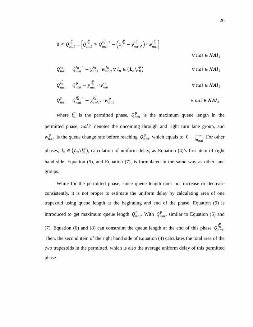
3.2.3.1 Lane Group without Permitted Left Turn. According to HCM 2010 method, the
calculation of uniform delay for a lane group is based on the area bounded the polygon
shown in Figure 1, which is used for lane groups that do not have permitted left turn. The
set of all lane groups that have no permitted left turn is denoted as 𝑵𝑨𝑰1.
21
Figure 3.1. Uniform Delay Shape for Normal Lane Groups
Figure 3.1 is a polygon shape that illustrate the uniform delay for a through and
right turn lane group with a 4-phase signal timing plan. 𝑄𝑛𝑛𝑛𝑙𝑛 is the queue length of this
lane group at the end of phase 𝑙𝑛. 𝑤𝑛𝑛𝑛𝑙𝑛 is the queue change rate and 𝑦𝑛𝑛𝑛
𝑙𝑛 is the queue
change duration.
The area bounded by the polygon represents the total uniform delay, and then the
total is divided by the number of arrivals per cycle to estimate the average uniform delay.
Thus, in HCM 2010, these calculations are summarized in the equations below.
𝑑𝑛𝑛𝑛1 =∑ �0.5 ∙ (𝑄𝑛𝑛𝑛
𝑙𝑛−1 + 𝑄𝑛𝑛𝑛𝑙𝑛 ) ∙ 𝑦𝑛𝑛𝑛
𝑙𝑛 �𝑙𝑛𝑣𝑛𝑛𝑛𝜔𝑛
,∀ 𝑛𝑎𝑖 ∈ 𝑵𝑨𝑰1
𝑄𝑛𝑛𝑛𝑙𝑛 = 𝑄𝑛𝑛𝑛
𝑙𝑛−1 − 𝑦𝑛𝑛𝑛𝑙𝑛 ∙ 𝑤𝑛𝑛𝑛
𝑙𝑛 ,∀ 𝑛𝑎𝑖 ∈ 𝑵𝑨𝑰1
𝑦𝑛𝑛𝑛𝑙𝑛 = min (𝑔𝑛
𝑙𝑛 ,𝑄𝑛𝑛𝑛𝑙𝑛−1
𝑤𝑛𝑛𝑛𝑙𝑛
),∀ 𝑙𝑛,∀ 𝑛𝑎𝑖 ∈ 𝑵𝑨𝑰1
Phase 1 Phase 2 Phase 3 Phase 4
𝑄𝑛𝑛𝑛1
𝑄𝑛𝑛𝑛2
𝑄𝑛𝑛𝑛3
𝑄𝑛𝑛𝑛4
𝑦𝑛𝑛𝑛4
𝑔𝑛4
Que
ue L
engt
h
Time
−𝑤 𝑛𝑙𝑛
𝑔𝑛3
𝑦𝑛𝑛𝑛3 𝑔𝑛2 𝑦𝑛𝑛𝑛2 𝑦𝑛𝑛𝑛1
𝑔𝑛1
22
In which, the queue change (build-up or vanish) rate, 𝑤𝑛𝑛𝑛𝑙𝑛 = 𝑠𝑛𝑛𝑛
𝑙𝑛 − 𝑣𝑛𝑎𝑛𝑙𝑛𝑙𝑚𝑛𝑎𝑛
, and
𝑄𝑛𝑛𝑛𝑙𝑛−1 denotes the queue length at the end of 𝑙𝑛’s previous phase. 𝑙𝑛𝑙𝑚𝑛𝑛𝑛 is the
number of lanes of this lane group. It has to be mentioned that Equation (1) is not
mathematically rigorous. For the phases that queue length decreases, 𝑤𝑛𝑛𝑛𝑙𝑛 > 0, the value
of the queue change duration 𝑦𝑛𝑛𝑛𝑙𝑛 is able to be successfully determined by Equation (3)
since the queue clearance time is nonnegative, 𝑄𝑛𝑎𝑛𝑙𝑛−1
𝑤𝑛𝑎𝑛𝑙𝑛 > 0; however, when queue length
does not decrease, such as phase 1, 2, or 3 in Figure 1, item 𝑄𝑛𝑎𝑛𝑙𝑛−1
𝑤𝑛𝑎𝑛𝑙𝑛 will be either negative
or meaningless since queue change rate 𝑤𝑛𝑛𝑛𝑙𝑛 is not positive in this case. The negative
value of the queue clearance time, 𝑄𝑛𝑎𝑛𝑙𝑛−1
𝑤𝑛𝑎𝑛𝑙𝑛 , will lead to a negative value of queue change
duration, 𝑦𝑛𝑛𝑛𝑙𝑛 , due to the minimum logic, which contradicts with the fact that queue
change duration should always be nonnegative. In addition, item 𝑄𝑛𝑎𝑛𝑙𝑛−1
𝑤𝑛𝑎𝑛𝑙𝑛 will become
meaningless in mathematical model when queue change rate 𝑤𝑛𝑛𝑛𝑙𝑛 = 0. Thus, in order to
keep the consistency of the formulation, the minimum logic in the original model has to
be replaced by other mathematical logic that is more rigorous.
In this study, the following equations are proposed.
𝑑𝑛𝑛𝑛1 ∙ 𝑣𝑛𝑛𝑛 ∙ 𝜔𝑛 = ��0.5 ∙ (𝑄𝑛𝑛𝑛𝑙𝑛−1 + 𝑄𝑛𝑛𝑛
𝑙𝑛 ) ∙ 𝑦𝑛𝑛𝑛𝑙𝑛 �
𝑙𝑛
,∀ 𝑛𝑎𝑖 ∈ 𝑵𝑨𝑰1
𝑄𝑛𝑛𝑛𝑙𝑛 = max (0,𝑄𝑛𝑛𝑛
𝑙𝑛−1 − 𝑔𝑛𝑙𝑛 ∙ 𝑤𝑛𝑛𝑛
𝑙𝑛 ),∀ 𝑙𝑛,∀ 𝑛𝑎𝑖 ∈ 𝑵𝑨𝑰1
𝑄𝑛𝑛𝑛𝑙𝑛 = 𝑄𝑛𝑛𝑛
𝑙𝑛−1 − 𝑦𝑛𝑛𝑛𝑙𝑛 ∙ 𝑤𝑛𝑛𝑛
𝑙𝑛 ,∀ 𝑙𝑛,∀ 𝑛𝑎𝑖 ∈ 𝑵𝑨𝑰1
When observing the value of the queue length at the end of a phase, 𝑄𝑛𝑛𝑛𝑙𝑛 , there are
23
only two potential results: 1) 0, if queue fully cleared during this phase, and in this case,
𝑄𝑛𝑛𝑛𝑙𝑛 ≥ 𝑄𝑛𝑛𝑛
𝑙𝑛−1 − 𝑔𝑛𝑙𝑛 ∙ 𝑤𝑛𝑛𝑛
𝑙𝑛 , or 2) 𝑄𝑛𝑛𝑛𝑙𝑛−1 − 𝑔𝑛
𝑙𝑛 ∙ 𝑤𝑛𝑛𝑛𝑙𝑛 , if queue is not able to be cleared
during this phase, and in this case, it can be either shortening , 𝑤𝑛𝑛𝑛𝑙𝑛 ≥ 0, or building the
queue, 𝑤𝑛𝑛𝑛𝑙𝑛 ≤ 0. Thus, with Equation (2), 𝑄𝑛𝑛𝑛
𝑙𝑛 can be successfully obtained with any
value of queue change rate 𝑤𝑛𝑛𝑛𝑙𝑛 . Queue change duration 𝑦𝑛𝑛𝑛
𝑙𝑛 is then constrained in
Equation (3), and will be ranged between 0 and phase length 𝑔𝑛𝑙𝑛 internally. Therefore,
the proposed equations cover all the possible situations in practice, and can be used to
replace the minimum condition in the original formula.
The second equation can be modified into the simple complementarity conditions
shown as follow.
0 ≤ 𝑄𝑛𝑛𝑛𝑙𝑛 ⊥ �𝑄𝑛𝑛𝑛
𝑙𝑛 ≥ 𝑄𝑛𝑛𝑛𝑙𝑛−1 − 𝑔𝑛
𝑙𝑛 ∙ 𝑤𝑛𝑛𝑛𝑙𝑛 �,∀ 𝑙𝑛,∀ 𝑛𝑎𝑖 ∈ 𝑵𝑨𝑰1
The above complementarity constraints hold only if at least one of the following holds.
0 ≤ 𝑄𝑛𝑛𝑛𝑙𝑛 ,𝑄𝑛𝑛𝑛
𝑙𝑛 = 𝑄𝑛𝑛𝑛𝑙𝑛−1 − 𝑔𝑛
𝑙𝑛 ∙ 𝑤𝑛𝑛𝑛𝑙𝑛
0 = 𝑄𝑛𝑛𝑛𝑙𝑛 ,𝑄𝑛𝑛𝑛
𝑙𝑛 ≥ 𝑄𝑛𝑛𝑛𝑙𝑛−1 − 𝑔𝑛
𝑙𝑛 ∙ 𝑤𝑛𝑛𝑛𝑙𝑛
To identify the previous phase of phase 𝑙𝑛, incidence matrix 𝚭, in which element
𝜁𝑛𝑛𝑛𝑙𝑛′,𝑙𝑛 = 1, if phase 𝑙𝑛
′ is the previous phase of 𝑙𝑛 (𝑙𝑛′, 𝑙𝑛 ∈ 𝑳𝑛 ) in one cycle, 0
otherwise, is introduced in the proposed model. The calculation of uniform delay is started
from the first red light phase, and it is assumed that there is no initial queue, which means
the queue length at the beginning of the first red light phase is 0. Thus, in order to achieve
this, for the first red light phase of any lane group, all the elements are 0.
24
𝑄𝑛𝑛𝑛𝑙𝑛−1 = �𝜁𝑛𝑛𝑛
𝑙𝑛′,𝑙𝑛 ∙ 𝑄𝑛𝑛𝑛𝑙𝑛′
𝑙𝑛′
By using HCM 2010 method, the calculation of incremental delay can be
formulated as
𝑑𝑛𝑛𝑛2 = 900𝑇 ��𝑣𝑛𝑛𝑛�̅�𝑛𝑛𝑛
− 1� + �(𝑣𝑛𝑛𝑛�̅�𝑛𝑛𝑛
− 1)2 +4𝑣𝑛𝑛𝑛�̅�𝑛𝑛𝑛2𝑇
� ,∀ 𝑛𝑎𝑖 ∈ 𝑵𝑨𝑰1
where
�̅�𝑛𝑛𝑛 = 𝑙𝑛𝑙𝑚𝑛𝑛𝑛 × �(𝑠𝑛𝑛𝑛𝑙𝑛 ×
𝑔𝑛𝑙𝑛
𝜔𝑛)
𝑙𝑛
,∀ 𝑛𝑎𝑖 ∈ 𝑵𝑨𝑰1
Since the capacity of lane group 𝑖, �̅�𝑛𝑛𝑛, is a variable and always non-negative, in
order to avoid numerical computation issues as �̅�𝑛𝑛𝑛 = 0, we modify the original