1316 IEEE TRANSACTIONS ON AUTOMATIC CONTROL, VOL. 59, NO. 5, MAY 2014
Optimal Stabilization Using Lyapunov Measures
Arvind Raghunathan and Umesh Vaidya
Abstract—Numerical solutions for the optimal feedback stabilization ofdiscrete time dynamical systems is the focus of this technical note. Set-the-oretic notion of almost everywhere stability introduced by the Lyapunovmeasure, weaker than conventional Lyapunov function-based stabilizationmethods, is used for optimal stabilization. The linear Perron-Frobeniustransfer operator is used to pose the optimal stabilization problem as aninfinite dimensional linear program. Set-oriented numerical methods areused to obtain the finite dimensional approximation of the linear program.We provide conditions for the existence of stabilizing feedback controls andshow the optimal stabilizing feedback control can be obtained as a solutionof a finite dimensional linear program. The approach is demonstrated onstabilization of period two orbit in a controlled standard map.
Index Terms—Almost everywhere stability, numerical methods, optimalstabilization.
I. INTRODUCTION
Stability analysis and stabilization of nonlinear systems are two ofthe most important, extensively studied problems in control theory.Lyapunov functions are used for stability analysis and control Lya-punov functions (CLF) are used in the design of stabilizing feedbackcontrollers. Under the assumption of detectability and stabilizability ofthe nonlinear system, a positive valued optimal cost function of an op-timal control problem (OCP) can also be used as a control Lyapunovfunction. The optimal controls of OCP are obtained as the solution ofthe Hamilton Jacobi Bellman (HJB) equation. The HJB equation is anonlinear partial differential equation and one must resort to approxi-mate numerical schemes for its solution. Numerical schemes typicallydiscretize the state-space; hence, the resulting problem size grows ex-ponentially with the dimension of the state-space. This is commonlyreferred to as the curse of dimensionality. The approach is particularlyattractive for feedback control of nonlinear systems with lower dimen-sional state space. The method proposed in this technical note also suf-fers from the same drawback. Among the vast literature available onthe topic of solving the HJB equation, we briefly review some of therelated literature.Vinter [1] was the first to propose a linear programming approach
for nonlinear optimal control of continuous time systems. This wasexploited to develop a numerical algorithm, based on semidefiniteprogramming and density function-based formulation by Rantzer andco-workers in [2], [3]. Global almost everywhere stability of stochasticsystems was studied by van Handel [4], using the density function.Lasserre, Hernández-Lerma, and co-workers [5], [6] formulated thecontrol of Markov processes as a solution of the HJB equation. Anadaptive space discretization approach is used in [7]; a cell mapping
Manuscript received November 22, 2011; revised July 10, 2012; acceptedOctober 06, 2013. Date of publication November 06, 2013; date of currentversion April 18, 2014. This work was supported by the NSF under grantsCMMI-0807666 and ECCS-1002053. Recommended by Associate Editor A.Ozdaglar.A. Raghunathan is with Mitsubishi Electric Research Laboratories, Cam-
bridge, MA 02139 USA (e-mail: [email protected]; [email protected]).U. Vaidya is with the Department of Electrical & Computer Engineering,
Iowa State University, Ames, IA 50011 USA (e-mail: [email protected]).Color versions of one or more of the figures in this technical note are available
online at http://ieeexplore.ieee.org.Digital Object Identifier 10.1109/TAC.2013.2289707
approach is used in [8] and [9], [10] utilizes set oriented numericalmethods to convert the HJB to one of finding the minimum cost pathon a graph derived from transition. In [11]–[13], solutions to stochasticand deterministic optimal control problems are proposed, using alinear programming approach or using a sequence of LMI relaxations.Our technical note also draws some connection to research on opti-mization and stabilization of controlled Markov chains discussed in[14]. Computational techniques based on the viscosity solution of theHJB equation is proposed for the approximation of value function andoptimal controls in [15] (Chapter VI).Our proposed method, in particular the computational approach,
draws some similarity with the above discussed references on theapproximation of the solution of the HJB equation [8]–[10], [15].Our method, too, relies on discretization of state space to obtainglobally optimal stabilizing control. However, our proposed approachdiffers from the above references in the following two fundamentalways. The first main difference arises due to adoption of non-classicalweaker set-theoretic notion of almost everywhere stability for optimalstabilization. This weaker notion of stability allows for the existenceof unstable dynamics in the complement of the stabilized attractor set;whereas, such unstable dynamics are not allowed using the classicalnotion of Lyapunov stability adopted in the above references. Thisweaker notion of stability is advantageous from the point of view offeedback control design. The notion of almost everywhere stabilityand density function for its verification was introduced by Rantzer in[16]. Furthermore, Rantzer proved, that unlike the control Lyapunovfunction, the co-design problem of jointly finding the density functionand the stabilizing controller is convex [17]. The Lyapunov measureused in this technical note for optimal stabilization can be viewed asa measure corresponding to the density function [18], [19]. Hence,it enjoys the same convexity property for the controller design. Thisconvexity property, combined with the proposed linear transfer oper-ator framework, is precisely exploited in the development of linearprogramming-based computational framework for optimal stabiliza-tion using Lyapunov measures. The second main difference comparedto [14] and [15] is in the use of the discount factor in the costfunction (refer to Remark 9). The discount factor plays an importantrole in controlling the effect of finite dimensional discretization or theapproximation process on the true solution. In particular, by allowingfor the discount factor, , to be greater than one, it is possible to ensurethat the control obtained using the finite dimensional approximation istruly stabilizing the nonlinear system [20], [21].In a previous work [20] involving Vaidya, the problem of de-
signing deterministic feedback controllers for stabilization via controlLyapunov measure was addressed. The authors proposed solvingthe problem by using a mixed integer formulation or a non-convexnonlinear program, which are not computationally efficient. Thereare two main contributions of this technical note. First, we showa deterministic stabilizing feedback controller can be constructedusing a computationally cheap tree-growing algorithm (Algorithm1, Lemma 11). The second main contribution of this technical noteis the extension of the Lyapunov measure framework introduced in[18] to design optimal stabilization of an attractor set. We prove theoptimal stabilizing controllers can be obtained as the solution to alinear program. Unlike the approach proposed in [20], the solutionto the linear program is guaranteed to yield deterministic controls.This technical note is an extended version of the technical note thatappeared in the 2008 American Control Conference [22].This technical note is organized as follows. In Section II, we provide
a brief overview of key results from [18] and [20] for stability anal-ysis, and stabilization of nonlinear systems using the Lyapunov mea-
IEEE TRANSACTIONS ON AUTOMATIC CONTROL, VOL. 59, NO. 5, MAY 2014 1317
sure. The transfer operators-based framework is used to formulate theOCP as an infinite dimensional linear program in Section III. A com-putational approach, based on set-oriented numerical methods, is pro-posed for the finite dimensional approximation of the linear programin Section IV. Simulation results are presented in Section V, followedby conclusions in Section VI.
II. LYAPUNOV MEASURE, STABILITY AND STABILIZATION
The Lyapunov measure and control Lyapunov measure were intro-duced in [18], [20] for stability analysis and stabilizing controller de-sign in discrete-time dynamical systems of the form,
(1)
where is assumed to be continuous with , a com-pact set. We denote by the Borel- algebra on and ,the vector space of a real valued measure on . The mapping, ,is assumed to be nonsingular with respect to the Lebesgue measure ,i.e., , for all sets , such that .In this technical note, we are interested in optimal stabilization of anattractor set defined as follows:Definition 1 (Attractor Set): A set is said to be forward
invariant under , if . A closed forward invariant set, , issaid to be an attractor set, if it there exists a neighborhood of, such that for all , where is the limit set of[18].Remark 2: In the following definitions and theorems, we will use
the notation, , to denote the neighborhood of the attractorset and , a finite measure absolutely continuous withrespect to Lebesgue.Definition 3 (Almost Everywhere Stable With Geometric Decay):
The attractor set for a dynamical system (1) is said to be almosteverywhere (a.e.) stable with geometric decay with respect to some fi-nite measure, , if given any , there existsand , such that .The above set-theoretic notion of a.e. stability is introduced in [18]
and verified by using the linear transfer operator framework. For thediscrete time dynamical system (1), the linear transfer Perron Frobenius(P-F) operator [23] denoted by is given by,
(2)
where is the indicator function supported on the setand is the inverse image of set . We define a sub-stochasticoperator as a restriction of the P-F operator on the complement of theattractor set as follows:
(3)
for any set and . The condition for the a.e.stability of an attractor set with respect to some finite measure isdefined in terms of the existence of the Lyapunov measure , definedas follows [18]Definition 4 (Lyapunov Measure): The Lyapunov measure is de-
fined as any non-negative measure , finite outside (see Remark2), and satisfies the following inequality, , forsome and all sets , such that .The following theorem from [24] provides the condition for a.e. sta-
bility with geometric decay.Theorem 5: An attractor set for the dynamical system (1) is a.e.
stable with geometric decay with respect to finite measure , if and
only if for all there exists a non-negative measure , which isfinite on and satisfies
(4)
for all measurable sets and for some .Proof: We refer readers to Theorem 5 from [21] for the proof.
We consider the stabilization of dynamical systems of the form, where and
are the state and the control input, respectively. Both and areassumed compact. The objective is to design a feedback controller,
, to stabilize the attractor set . The stabilizationproblem is solved using the Lyapunov measure by extending theP-F operator formalism to the control dynamical system [20]. Wedefine the feedback control mapping as
. We denote by the Borel- algebra onand the vector space of real valued measures on . For any
, the control mapping can be used to define a measure,, as follows:
(5)
for all sets and . Since is an injec-tive function with satisfying (5), it follows from the theoremon disintegration of measure [25] (Theorem 5.8) there existsa unique disintegration of the measure for almost all
, such that ,for any Borel-measurable function . In particular, for
, the indicator function for the set , we obtainUsing the
definition of the feedback controller mapping , we write the feed-back control system as . Thesystem mapping can be associated with P-F operators
as . TheP-F operator for the composition can be written as aproduct of and . In particular, we obtain [21]
The P-F operators, and , are used to define their restriction,, and
to the complement of the attractor set, respectively, in a way similar to(3). The control Lyapunov measure introduced in [20] is defined as anynon-negative measure , finite on , such thatthere exists a control mapping that satisfies ,for every set and . Stabilization of the attractorset is posed as a co-design problem of jointly obtaining the control Lya-punov measure and the control P-F operator or in particular dis-integration of measure , i.e., . The disintegration measure , whichlives on the fiber of , in general, will not be absolutely continuouswith respect to Lebesgue. For the deterministic control map, , theconditional measure, , the Dirac delta measure.However, for the purpose of computation, we relax this condition. Thepurpose of this technical note and the following sections are to extendthe Lyapunov measure-based framework for the optimal stabilizationof nonlinear systems. One of the key highlights of this technical noteis the deterministic finite optimal stabilizing control is obtained as thesolution for a finite linear program.
1318 IEEE TRANSACTIONS ON AUTOMATIC CONTROL, VOL. 59, NO. 5, MAY 2014
III. OPTIMAL STABILIZATION
The objective is to design a feedback controller for the stabilizationof the attractor set, , in a.e. sense, while minimizing a suitable costfunction. Consider the following control system:
(6)
where and are state and control input,respectively, and . Both and are assumedcompact. We define .Assumption 6: We assume there exists a feedback controller map-
ping , which locally stabilizes the invariant set ,i.e., there exists a neighborhood of such that and
for all ; moreover .Our objective is to construct the optimal stabilizing controller for
almost every initial condition starting from . Letbe the stabilizing control map for . The control mapping
can be written as follows:
forfor .
(7)
Furthermore, we assume the feedback control systemis non-singular with respect to the Lebesgue measure, . We seek
to design the controller mapping, , such that theattractor set is a.e. stable with geometric decay rate , whileminimizing the following cost function,
(8)
where , the cost function is assumed a continuousnon-negative real-valued function, such that ,
, and . Note, that in the cost function (8), isallowed greater than one and this is one of the main departures from theconventional optimal control problem, where . However, underthe assumption that the controller mapping renders the attractor seta.e. stable with a geometric decay rate, , the cost function (8) isfinite.Remark 7: To simplify the notation, in the following we will use the
notion of the scalar product between continuous functionand measure as [23].The following theorem proves the cost of stabilization of the set
as given in (8) can be expressed using the control Lyapunov measureequation.Theorem 8: Let the controller mapping, , be
such that the attractor set for the feedback control systemis a.e. stable with geometric decay rate . Then, the
cost function (8) is well defined for and, furthermore, the costof stabilization of the attractor set with respect to Lebesgue almostevery initial condition starting from set can be expressedas follows:
(9)
where, and is the solution of the following control Lya-punov measure equation:
(10)
for all and where is a finite measuresupported on the set .
Proof: The proof is omitted in this technical note, due to limitedspace but can be found in the online version of the technical note [21](Theorem 8).
By appropriately selecting the measure on the right-hand side of thecontrol Lyapunov measure equation (10) (i.e., ), stabilization of theattractor set with respect to a.e. initial conditions starting from a par-ticular set can be studied. The minimum cost of stabilization is definedas the minimum over all a.e. stabilizing controller mappings, , witha geometric decay as follows:
(11)
Next, we write the infinite dimensional linear program for the optimalstabilization of the attractor set . Towards this goal, we first define theprojection map, as: and denote theP-F operator corresponding to as ,which can be written as
. Using this definition of projection mapping,, and the corresponding P-F operator, we can write the linear pro-
gram for the optimal stabilization of set with unknown variable asfollows:
(12)for .Remark 9: Observe the geometric decay parameter satisfies .
This is in contrast to most optimization problems studied in the contextof Markov-controlled processes, such as in Lasserre and Hernández-Lerma [5]. Average cost and discounted cost optimality problems areconsidered in [5], [15]. The additional flexibility provided byguarantees the controller obtained from the finite dimensional approx-imation of the infinite dimensional program (12) also stabilizes the at-tractor set for system (6). For a more detailed discussion on the roleof on the finite dimensional approximation, we refer readers to theonline version of the technical note [21].
IV. COMPUTATIONAL APPROACH
The objective of the present section is to present a computationalframework for the solution of the finite-dimensional approximation ofthe optimal stabilization problem in (12). There exists a number of ref-erences related to the solution of infinite dimensional linear programs(LPs), in general, and those arising from the control of Markov pro-cesses. Some will be described next. The monograph by Anderson andNash [26] is an excellent reference on the properties of infinite dimen-sional LPs.Our intent is to use the finite-dimensional approximation as a tool to
obtain stabilizing controls to the infinite-dimensional system. First, wewill derive conditions under which solutions to the finite-dimensionalapproximation exist.Following [18] and [20], we discretize the state-space and control
space for the purposes of computations as described below. Borrowingthe notation from [20], let denote afinite partition of the state-space . The measure space as-sociated with is . We assume without loss of generality thatthe attractor set, , is contained in , that is, . Simi-larly, the control space, , is quantized and the control input is as-sumed to take only finitely many control values from the quantizedset, , where . The partition,
, is identified with the vector space, . The system map thatresults from choosing the controls is denoted as and the cor-responding P-F operator is denoted as . Fixing thecontrols on all sets of the partition to , i.e., , for all
, the system map that results is denoted as with the cor-responding P-F operator denoted as . The entries for
are calculated as: , where isthe Lebesgue measure and denotes the -th entry of the
IEEE TRANSACTIONS ON AUTOMATIC CONTROL, VOL. 59, NO. 5, MAY 2014 1319
matrix. Since , we have is a Markov matrix. Ad-ditionally, will denote the finite dimensionalcounterpart of the P-F operator restricted to , the complementof the attractor set. It is easily seen that consists of the firstrows and columns of .In [18] and [20], stability analysis and stabilization of the attractor
set are studied, using the above finite dimensional approximation of theP-F operator. The finite dimensional approximation of the P-F operatorresults in a weaker notion of stability, referred to as coarse stability[18], [21]. Roughly speaking, coarse stability means stability moduloattractor sets with domain of attraction smaller than the size of cellswithin the partition.With the above quantization of the control space and partition of the
state space, the determination of the control (or equivalently) for all has now been cast as a problem of choosing
for all sets . The finite dimensional ap-proximation of the optimal stabilization problem (12) is equivalent tosolving the following finite-dimensional LP:
(13)
where we have used the notation for the transpose operation,and denote the support of Lebesgue measure, ,
on the set , is the cost defined on withthe cost associated with using control action on set ;
are, respectively, the discrete counter-parts of infinite-dimensional measure quantities in (12). In the LP (13), we have notenforced the constraint,
(14)
for each . The above constraint ensures the controlon each set in unique. We prove in the following the uniqueness can beensured without enforcing the constraint, provided the LP (13) has asolution. To this end, we introduce the dual LP associated with the LPin (13). The dual to the LP in (13) is,
(15)
In the above LP (15), is the dual variable to the equality constraintsin (13).
A. Existence of Solutions to the Finite LP
We make the following assumption throughout this section.Assumption 10: There exists , such
that the LP in (13) is feasible for some .Note, Assumption 10 does not impose the requirement in (14). For
the sake of simplicity and clarity of presentation, we will assume thatthe measure, , in (13) is equivalent to the Lebesgue measure and. Satisfaction of Assumption 10 can be verified using the followingalgorithm.Algorithm 1: 1) Set , , . 2) Set
. 3) For each do a) Pick the smallestsuch that for some . b) If
exists then, set , . 4) End For 5) Ifthen, set . STOP. 6) If then,
STOP. 7) Set . Go to Step 2.The algorithm iteratively adds to , set , which has a non-zero
probability of transition to any of the sets in . In graph theory terms,the above algorithm iteratively builds a tree starting with the set. If the algorithm terminates in Step 6, then we have identified sets
that cannot be stabilized with the controls in . Ifthe algorithm terminates at Step 5, then we show in the Lemma belowthat a set of stabilizing controls exist.Lemma 11: Let be a partition of the state
space, , and be a quantization of the con-trol space, . Suppose Algorithm 1 terminates in Step 5 afteriterations, then the controls identified by the algorithm renders thesystem coarse stable.
Proof: Let represent the closed loop transition matrixresulting from the controls identified by Algorithm 1. Suppose
, be any initial distribution supported onthe complement of the attractor set . By construction,has a non-zero probability of entering the attractor set aftertransitions. Hence,
Thus, the sub-Markov matrix is transient and implies the claim.
Algorithm 1 is less expensive than the approaches proposed in [20],where a mixed integer LP and a nonlinear programming approach wereproposed. The strength of our algorithm is that it is guaranteed to finddeterministic stabilizing controls, if they exist. The following lemmashows an optimal solution to (13) exists under Assumption 10.Lemma 12: Consider a partition of
the state-space with attractor set and a quantizationof the control space . Suppose Assumption 10
holds for some and for . Then, there exists an optimalsolution, , to the LP (13) and an optimal solution, , to the dual LP(15) with equal objective values, ( ) andbounded.
Proof: From Assumption 10, the LP (13) is feasible. Observethe dual LP in (15) is always feasible with a choice of . Thefeasibility of primal and dual linear programs implies the claim as aresult of LP strong duality [27].Remark 13: Note, existence of an optimal solution does not impose
a positivity requirement on the cost function, . In fact, even assigningallows determination of a stabilizing control from the Lyapunov
measure (13). In this case, any feasible solution to (13) suffices.The next result shows the LP (13) always admits an optimal solution
satisfying (14).Lemma 14: Given a partition of the state-
space, , with attractor set, , and a quantization,, of the control space, . Suppose Assumption 10 holds
for some and for . Then, there exists a solutionsolving (13) and solving (15) for any
. Further, the following hold at the solution: 1) For each, there exists at least one , such that
and . 2) There exists
a that solves (13), such that for each , there isexactly one , such that andfor .
Proof: From the assumptions, we have that Lemma 12 holds.Hence, there exists solving (13) and solving(15) for any . Further, and satisfy following thefirst-order optimality conditions [27],
(16)
We will prove each of the claims in order.
1320 IEEE TRANSACTIONS ON AUTOMATIC CONTROL, VOL. 59, NO. 5, MAY 2014
Claim 1: Suppose, there exists , such thatfor all . Substituting in the optimality con-
ditions (16), one obtains,
which cannot hold, since, has non-negative entries, and. Hence, there exists at least one such that .
The complementarity condition in (16) then requires that. This proves the first claim.
Claim 2: Denote for each. The existence of for each follows from statement
1. Define and as follows:
(17)
for all . From the definition of , and thecomplementarity condition in (16), it is easily seen that satisfies
(18)
Since is bounded and , it follows that . Defineas,
... (19a)
(19b)
The above is well-defined, since we have already shown that.From the construction of , we have that for each there exists only
one , namely , for which . It remains to show thatsolves (13). For this, observe
(20)
The primal and dual objectives are equal with the above definition of. Hence, solves (13). The claim is proved.The following theorem states the main result.Theorem 15: Consider a partition of the
state-space, , with attractor set, , and a quantization,, of the control space, . Suppose Assumption 10 holds
for some and for . Then, the following statementshold: 1) there exists a bounded , a solution to (13) and a bounded , asolution to (15); 2) the optimal control for each set, ,is given by ; 3)satisfying
is the Lyapunov measure for the controlled system.Proof: Assumption 10 ensures that the linear programs (13) and
(15) have a finite optimal solution (Lemma (12)). This proves the firstclaim of the theorem and also allows the applicability of Lemma 14.The remaining claims follow as a consequence.Although the results in this section assumed the measure, , is
equivalent to Lebesgue, this can be easily relaxed to the case whereis absolutely continuous with respect to Lebesgue and is of interest
where the system is not everywhere stabilizable. If it is known thereare regions of the state-space not stabilizable, then can be chosen
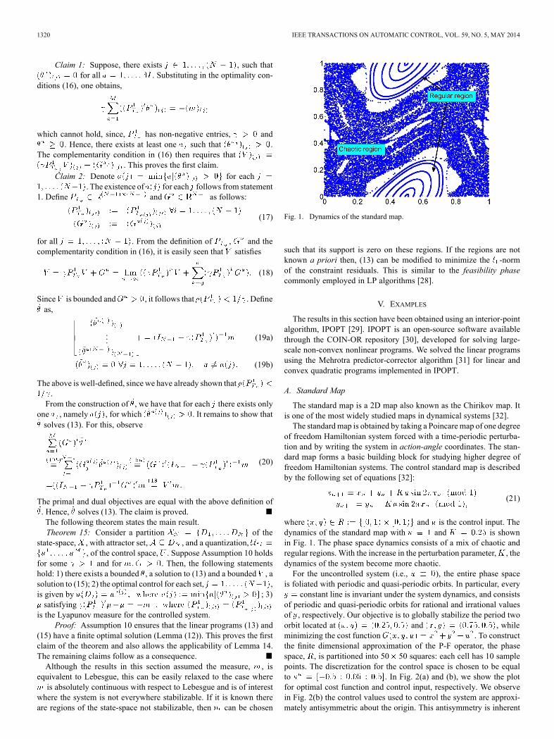
Fig. 1. Dynamics of the standard map.
such that its support is zero on these regions. If the regions are notknown a priori then, (13) can be modified to minimize the -normof the constraint residuals. This is similar to the feasibility phasecommonly employed in LP algorithms [28].
V. EXAMPLES
The results in this section have been obtained using an interior-pointalgorithm, IPOPT [29]. IPOPT is an open-source software availablethrough the COIN-OR repository [30], developed for solving large-scale non-convex nonlinear programs. We solved the linear programsusing the Mehrotra predictor-corrector algorithm [31] for linear andconvex quadratic programs implemented in IPOPT.
A. Standard Map
The standard map is a 2D map also known as the Chirikov map. Itis one of the most widely studied maps in dynamical systems [32].The standard map is obtained by taking a Poincare map of one degree
of freedom Hamiltonian system forced with a time-periodic perturba-tion and by writing the system in action-angle coordinates. The stan-dard map forms a basic building block for studying higher degree offreedom Hamiltonian systems. The control standard map is describedby the following set of equations [32]:
(21)
where and is the control input. Thedynamics of the standard map with and is shownin Fig. 1. The phase space dynamics consists of a mix of chaotic andregular regions. With the increase in the perturbation parameter, , thedynamics of the system become more chaotic.For the uncontrolled system (i.e., ), the entire phase space
is foliated with periodic and quasi-periodic orbits. In particular, everyconstant line is invariant under the system dynamics, and consists
of periodic and quasi-periodic orbits for rational and irrational valuesof , respectively. Our objective is to globally stabilize the period twoorbit located at and , whileminimizing the cost function . To constructthe finite dimensional approximation of the P-F operator, the phasespace, , is partitioned into 50 50 squares: each cell has 10 samplepoints. The discretization for the control space is chosen to be equalto . In Fig. 2(a) and (b), we show the plotfor optimal cost function and control input, respectively. We observein Fig. 2(b) the control values used to control the system are approxi-mately antisymmetric about the origin. This antisymmetry is inherent
IEEE TRANSACTIONS ON AUTOMATIC CONTROL, VOL. 59, NO. 5, MAY 2014 1321
Fig. 2. (a) Optimal cost function. (b) Optimal control input.
in the standard map and can also be observed in the uncontrolled stan-dard map plot in Fig. 2(b).
VI. CONCLUSIONS
Lyapunovmeasure is used for the optimal stabilization of an attractorset for a discrete time dynamical system. The optimal stabilizationproblem using a Lyapunov measure is posed as an infinite dimensionallinear program. A computational framework based on set oriented nu-merical methods is proposed for the finite dimensional approximationof the linear program.The set-theoretic notion of a.e. stability introduced by the Lyapunov
measure offers several advantages for the problem of stabilization.First, the controller designed using the Lyapunov measure exploitsthe natural dynamics of the system by allowing the existence ofunstable dynamics in the complement of the stabilized set. Second, theLyapunov measure provides a systematic framework for the problemof stabilization and control of a system with complex non-equilibriumbehavior.
ACKNOWLEDGMENT
The authors would like to acknowledge A. Diwadkar from IowaState University for help with the simulation. We also thank an anony-mous referee of the previous version of the technical note for improvingthe its quality.
REFERENCES[1] R. B. Vinter, “Convex duality and nonlinear optimal control,” SIAM J.
Control Optimizat., vol. 31, pp. 518–538, 1993.[2] S. Hedlund and A. Rantzer, “Convex dynamic programming for hybrid
[3] S. Prajna and A. Rantzer, “Convex programs for temporal verificationof nonlinear dynamical systems,” SIAM J. Control Optimizat., vol. 46,no. 3, pp. 999–1021, 2007.
[4] R. Van Handel, “Almost global stochastic stability,” SIAM J. ControlOptimizat., vol. 45, pp. 1297–1313, 2006.
[5] O. Hernández-Lerma and J. B. Lasserre, Discrete-time Markov ControlProcesses: Basic Optimality Criteria. New York: Springer-Verlag,1996.
[6] O. Hernández-Lerma and J. B. Lasserre, “Approximation schemesfor infinite linear programs,” SIAM J. Optimizat., vol. 8, no. 4, pp.973–988, 1998.
[7] L. Grüne, “Error estimation and adaptive discretization for the discretestochastic Hamilton-Jacobi-Bellman equation,” Numerische Mathe-matik, vol. 99, pp. 85–112, 2004.
[8] L. G. Crespo and J. Q. Sun, “Solution of fixed final state optimal controlproblem via simple cell mapping,” Nonlinear Dynamics, vol. 23, pp.391–403, 2000.
[9] O. Junge and H. Osinga, “A set-oriented approach to global optimalcontrol,” ESAIM: Control, Optimisat. Calculus Variations, vol. 10, no.2, pp. 259–270, 2004.
[10] L. Grüne and O. Junge, “A set-oriented approach to optimal feedbackstabilization,” Syst. Control Lett., vol. 54, no. 2, pp. 169–180, 2005.
[11] D. Hernandez-Hernandez, O. Hernandez-Lerma, and M. Taksar, “Alinear programming approach to deterministic optimal control prob-lems,” Applicat. Mathemat., vol. 24, no. 1, pp. 17–33, 1996.
[12] V. Gaitsgory and S. Rossomakhine, “Linear programming approachto deterministic long run average optimal control problems,” SIAM J.Control Optimizat., vol. 44, no. 6, pp. 2006–2037, 2006.
[13] J. Lasserre, C. Prieur, and D. Henrion, “Nonlinear optimal control:Numerical approximation via moment and LMI-relaxations,” in Proc.IEEE Conf. Decision Control, Seville, Spain, 2005.
[14] S. Meyn, “Algorithm for optimization and stabilization of controlledMarkov chains,” Sadhana, vol. 24, pp. 339–367, 1999.
[15] M. Bardi and I. Capuzzo-Dolcetta, Optimal Control and ViscositySolutions of Hamilton-Jacobi-Bellman Equations. Boston, USA:Birkhauser, 1997.
[16] A. Rantzer, “A dual to Lyapunov’s stability theorem,” Syst. ControlLett., vol. 42, pp. 161–168, 2001.
[17] C. Prieur and L. Praly, “Uniting local and global controller,” in Proc.IEEE Conf. Decision Control, AZ, 1999, pp. 1214–1219.
[18] U. Vaidya and P. G. Mehta, “Lyapunov measure for almost everywherestability,” IEEE Trans. Automat. Control, vol. 53, pp. 307–323, 2008.
[19] R. Rajaram, U. Vaidya, M. Fardad, and B. Ganapathysubramanian,“Almost everywhere stability: Linear transfer operator approach,” J.Mathemat. Analys. Applicat., vol. 368, pp. 144–156, 2010.
[20] U. Vaidya, P. Mehta, and U. Shanbhag, “Nonlinear stabilization viacontrol Lyapunov measure,” IEEE Trans. Automat. Control, vol. 55,pp. 1314–1328, 2010.
[21] A. Raghunathan and U. Vaidya, Optimal Stabilization using LyapunovMeasures 2012 [Online]. Available: http://www.ece.iastate.edu/~ug-vaidya/publications.html
[22] A. Raghunathan and U. Vaidya, “Optimal stabilization using Lyapunovmeasure,” in Proc. Amer. Control Conf., Seattle, WA, USA, 2008, pp.1746–1751.
[23] A. Lasota and M. C. Mackey, Chaos, Fractals, and Noise: StochasticAspects of Dynamics. Berlin, Germany: Springer-Verlag, 1994.
[24] U. Vaidya, “Converse theorem for almost everywhere stability usingLyapunov measure,” in Proc. Amer. Control Conf., New York, NY,USA, 2007.
[25] H. Furstenberg, Recurrence in Ergodic Theory and CombinatorialNumber Theory. Princeton, NJ, USA: Princeton Univ. Press, 1981.
[26] E. Anderson and P. Nash, Linear Programming in Infinite-DimensionalSpaces – Theory and Applications. Chichester, U.K.: Wiley, 1987.
[27] O. L. Mangasarian, Nonlinear Programming. Philadelphia, PA,USA: Society for Industrial and Applied Mathematics (SIAM), 1994,vol. 10, Classics in Applied Mathematics.
[28] S. J. Wright, Primal-Dual Interior-Point Methods. Philadelphia, Pa,USA: Society for Industrial and Applied Mathematics, 1997.
[29] A. Wächter and L. T. Biegler, “On the implementaion of a primal-dualinterior point filter line search algorithm for large-scale nonlinear pro-gramming,” Mathemat. Programm., vol. 106, no. 1, pp. 25–57, 2006.
[30] COIN-OR Repository, [Online]. Available: http://www.coin-or.org/[31] J. Nocedal and S. Wright, Numerical Optimization Springer, 2006,
Springer series in operations research [Online]. Available: http://books.google.com/books?id=eNlPAAAAMAAJ
[32] U. Vaidya and I. Mezić, “Controllability for a class of area preservingtwist maps,” Physica D, vol. 189, pp. 234–246, 2004.