Research ArticleOptimal Urban Logistics Facility Location withConsideration of Truck-Related Greenhouse Gas EmissionsA Case Study of Shenzhen City
Mi Gan 1234 Dandan Li12 Mingfei Wang12 Guangyuan Zhang 123
Shuai Yang12 and Jiyang Liu12
1School of Transportation and Logistics Southwest Jiaotong University Chengdu Sichuan China2National United Engineering Laboratory of Integrated and Intelligent TransportationSouthwest Jiaotong University Chengdu Sichuan China3National Engineering Laboratory of Big Data Application in Integrated TransportationSouthwest Jiaotong University Chengdu Sichuan China4Sino-US Global Logistics Institute Shanghai Jiaotong University Shanghai China
Correspondence should be addressed to Guangyuan Zhang gyzhangswjtueducn
Received 2 December 2017 Accepted 29 March 2018 Published 14 June 2018
Academic Editor Anna Vila
Copyright copy 2018 Mi Gan et al This is an open access article distributed under the Creative Commons Attribution License whichpermits unrestricted use distribution and reproduction in any medium provided the original work is properly cited
The logistics facility location is always involved with great deals of investment Its construction and operation also bring out a hugeamount of the greenhouse gas (GHG) emission due to the consumption of building materials energy the running of trucks andother logistics equipment Particularly trucking activities in the urban logistics networks (ULN) are a major source of GHG Thispaper aims to formulate an eco-facility location model to minimize both the total cost of ULN construction and operation and theGHG emissions of truck trips Based on the mathematical relations of GHG emissions rates and several macroscopic factors whichwe obtained by multivariate regression analysis on a large set of empirical trucking data in our previous research the data-drivenemissions rates estimation function is acquired Then we link the estimation function of each trip purpose by various kinds oflogistics facilities through a qualitative analysisThe eco-facility location problem ismodeled by integrating the pure facility locationmodel and the GHG emissions function The problem is first converted to a biobjective mixed-integer program and the ParticleSwarm Optimization algorithm is applied to solve the model Through experiments with real case the effectiveness of the modelsand algorithms is verifiedThe eco-facility locationmodel for ULN tends to obtain the environment-friendly location decision Ouranalytical results also verify the hypothesis that locations of facility do impact the relevant truck-related GHG emissions especiallyto transfer transport as well as inbound and outbound freight
1 Introduction
The logistics activity in urban areas is responsible for a signif-icant portion of the global greenhouse gas (GHG) emissions[1] Due to the rapid development of E-commerce the relatedGHG emissions share is increasing continuously ReducingGHG emissions in logistics sector is crucial to sustainableurban development Since the urban logistics network (ULN)is the backbone for carrying out all the logistics activities andsatisfying the logistics demand of the whole city investigatingthe emission sources of logistics activity in urban finding
out the relationship of the GHG emissions rate and thecorresponding source and constructing an optimal modelconsidering both economic and environmental factors arenecessary to reduce the logistics-related GHG emissions
On account of the emission source in ULN first weexplore the composition of a typicalULNGenerally theULNis involved with nodes and arcs The node stands for thefacility and the arc refers to the distribution path or flowin each supply-demand pair Therefore it is obvious that theGHG emissions in ULN come from the facilities (nodes inULN) and distribution flows (arcs in ULN) which include
HindawiMathematical Problems in EngineeringVolume 2018 Article ID 8439582 14 pageshttpsdoiorg10115520188439582
2 Mathematical Problems in Engineering
the construction and operation of facilities the running oftrucks and other freight carriers [2] Indeed the constructionand operation of the facility bring out a huge amount of GHGemissions due to the consumption of building materialsenergy and so forth The location of the facility is alsoinvolved with great deals of investment and will not beeasily relocated after the facility is constructed [3] For theaspect of truck-related GHG emissions trucks play a key rolein urban freight transport system and ULN [4] To reduceULN-related GHG emissions in cities various strategiesmay be considered to target to the aforementioned emissionsources With respect to the facility-emission sources sincethe relationship between emissions and inside activity of thefacility is not hard to estimate such as the electricity for runthe warehouse the diesel for forklift or package materialswe use in the warehouse it is obvious that minimizing thenumber and scale of facilities with satisfying the customerdemand as well as improving the energy efficiency can reducethe emissions [5] On the hand of reducing GHG emissionsof trucks the recent progress is mainly from the operationallevel [6] For instance we have the eco-routing problems andthe eco-traffic assignment problemThe former one is to findoptimal routes that promise tominimize fuel consumption orGHG emissions [7]The latter one is to incorporate the GHGemissions into the general traffic assignment models [8ndash10]However due to strict control regulations on truck trafficthe available truck routes in urban areas are often limitedonce the ULN design is fixed So it will be more efficient tooptimize the truck routes through the beginning the designstage of ULN rather than to optimize the truck routes afterthe important facility location is fixed (M Zhalechian et al2016) Then does the location of facility impact the GHGemission of ULN truck flow What is the interface betweenldquocharacteristics of locationrdquo and truck emissions The solu-tion of proposed questions may be used to relocate majorlogistics facilities which could potentially have far-reachingeffects in reducing long-term GHG emissions [11] Howeverthere is just limited knowledge about this field Aiming tofill such research gap we have investigated a large set ofempirical truck trajectory data developed a trip purposeimputation matrix to classify truck-related GHG emissionsand explored how the macroscopic trip would affect overallGHG emissions associated with each type of truck trips(X Liu and et al 2016) The mathematical relationshipsbetween GHG emissions and various kinds of trip purposespopulation density of origin nodesdestination nodes theEuclidean distance of each trip and vehicle kerb weightare captured through the multivariate regression analysisSome managerial insights are drawn from the findings yetthe mathematical representation of GHG emissions has notbeen applied to optimize the real logistics network in thecity
On the other hand the facility location problem as a hotissue in operations research has been investigated by numer-ous researchers and practitioners for centuries In additionthe location of logistics or supply chain facilities is an impor-tant composition With respect to the ECO facility locationproblem there are some related literatures about other kindsof facilities such as manufacturing facility and hydropower
location [12] For the logistics facility location problemconsidering carbon emissions Tang et al investigated thelogistics facility location model with consideration of eco-nomic costs services and CO2 emissions simultaneously[13] Wang et al formulated a multiobjective model for thesupply chain design problem in which the facility locationdecision is with environmental concerns [14] Elhedhli andMerrick modelled the relationship between emissions andvehicle weight and merged the emissions into the minimalcost objective by multiplying with the emissions cost [15]Some of other researchers also focus on traditional networkdesign with multiobjective and environmental aspects [1617] However the emissions rate is obtained by amacroscopicway Few of them explore the data-driven emissions functionthrough applying real truck trajectory data or consideringthe relationship between real truck trip emissions associatedwith various kinds of facilitiesWithwitness of above analysiswe attempted to propose a hypothesis that reasonable facilitylocation is able to reduce truck-related GHG emissionsFirst a group of GHG emissions functions by truck trip isdeveloped through analyzing the regressions results proposedin [18]Thenwe integrated theGHGemissions functions intothe logistics network design problem Similar to the modelstructure proposed by Wang et al [14] we constructed abiobjective eco-facility location model aiming to minimizethe total cost of facility location and truck-related GHGemissions simultaneously
The remainder of this paper is organized as followsThe data-driven emissions rate function the multiobjectivemodel and the solution algorithms are addressed in Sec-tion 2 In Section 3 we test the models and the algorithmsby real-case data Some managerial insights are drawn fromthe comparison and analysis of the results in Section 4 Theconclusion is given in Section 5
2 Models and Algorithms
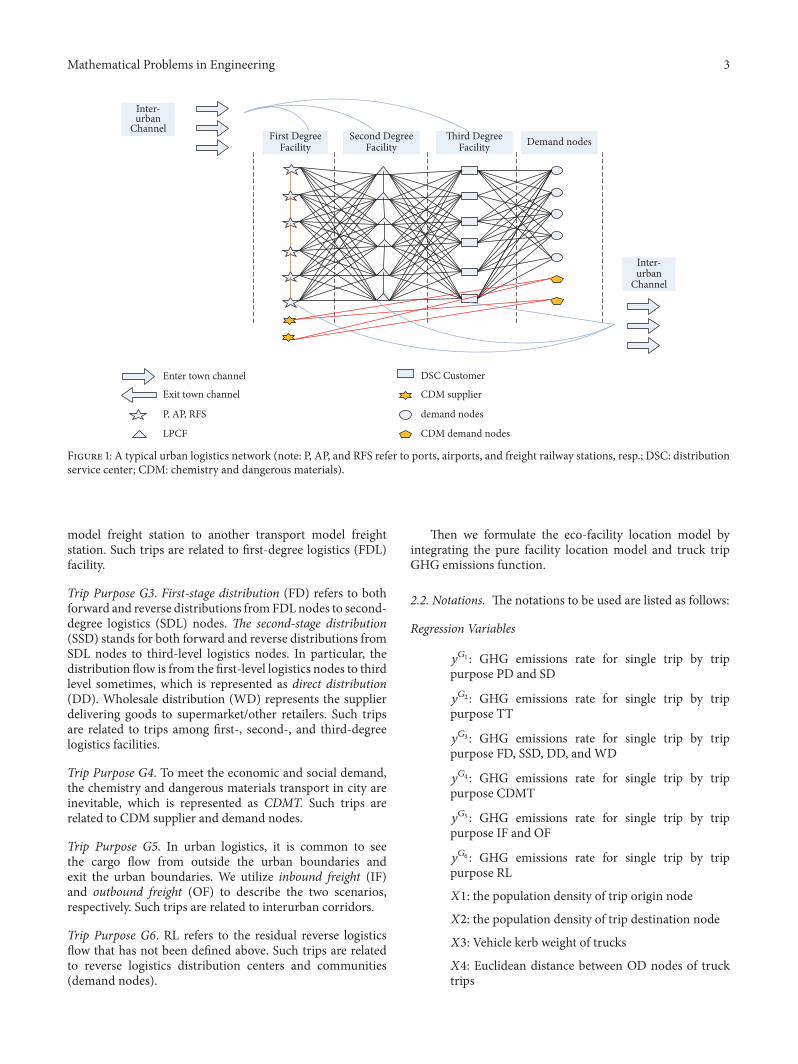
21 Classification of Logistics Flow In our research since thetruck trip purpose is directly linked with diverse kinds offacilities first we describe the relationship of trip purposeand facility following with the trip purpose classificationin previous research [18] Figure 1 shows a typical logisticsnetwork The trucks are running as a freight carrier on thearcs linking diverse kinds of facilities or demand nodestogether
The truck trip purpose in a ULN could be classifiedinto 6 groups and 11 types The trip purposes are stronglyrelated to the properties of origin and destination nodes Suchrelationships are described as follows
Trip Purpose G1 Urban parcel distribution (PD) consists ofboth personnel parcel and electronic commerce distributionSale distribution (SD) usually stands for the situation wherethe seller delivers the goods to final customers Such trips arerelated to the third-degree logistics facility and communities(demand nodes)
Trip Purpose G2 Multimodal transfer trip (TT) refers to thegoods and cargoes that are transferred from one transport
Mathematical Problems in Engineering 3
Enter town channel
P AP RFS
Exit town channel
LPCF
First DegreeFacility
Second DegreeFacility
Third DegreeFacility Demand nodes
Inter-urban
Channel
Inter-urban
Channel
DSC Customer
CDM supplier
CDM demand nodes
demand nodes
Figure 1 A typical urban logistics network (note P AP and RFS refer to ports airports and freight railway stations resp DSC distributionservice center CDM chemistry and dangerous materials)
model freight station to another transport model freightstation Such trips are related to first-degree logistics (FDL)facility
Trip Purpose G3 First-stage distribution (FD) refers to bothforward and reverse distributions fromFDLnodes to second-degree logistics (SDL) nodes The second-stage distribution(SSD) stands for both forward and reverse distributions fromSDL nodes to third-level logistics nodes In particular thedistribution flow is from the first-level logistics nodes to thirdlevel sometimes which is represented as direct distribution(DD) Wholesale distribution (WD) represents the supplierdelivering goods to supermarketother retailers Such tripsare related to trips among first- second- and third-degreelogistics facilities
Trip Purpose G4 To meet the economic and social demandthe chemistry and dangerous materials transport in city areinevitable which is represented as CDMT Such trips arerelated to CDM supplier and demand nodes
Trip Purpose G5 In urban logistics it is common to seethe cargo flow from outside the urban boundaries andexit the urban boundaries We utilize inbound freight (IF)and outbound freight (OF) to describe the two scenariosrespectively Such trips are related to interurban corridors
Trip Purpose G6 RL refers to the residual reverse logisticsflow that has not been defined above Such trips are relatedto reverse logistics distribution centers and communities(demand nodes)
Then we formulate the eco-facility location model byintegrating the pure facility location model and truck tripGHG emissions function
22 Notations The notations to be used are listed as follows
Regression Variables
1199101198661 GHG emissions rate for single trip by trippurpose PD and SD
1199101198662 GHG emissions rate for single trip by trippurpose TT
1199101198663 GHG emissions rate for single trip by trippurpose FD SSD DD and WD
1199101198664 GHG emissions rate for single trip by trippurpose CDMT
1199101198665 GHG emissions rate for single trip by trippurpose IF and OF
1199101198666 GHG emissions rate for single trip by trippurpose RL
1198831 the population density of trip origin node
1198832 the population density of trip destination node
1198833 Vehicle kerb weight of trucks1198834 Euclidean distance between OD nodes of trucktrips
119887119894 119887119895 119887119896 119887119897 1198871198971015840 119887ℎ operation costs for each facilityYuankg1199081 1199082 1199083 1199084 1199085 1199086 average trip load of trip pur-pose 1198661 1198662 1198663 1198664 1198665 1198666 respectively ton119863119898 119863119903119898 weekly demand of customers and weeklyreverse logistics demand of customers respectivelykg119863ℎ weekly demand of CDM demand nodes kg119874119894 119874119895 119874119896 119874119897 1198741198971015840 119874ℎ designed capacity of each facil-ity kg119873119894 119873119895 119873119896 119873119897 1198731198971015840 119873ℎ number of facilities119889119894119895 119889119894119896 119889119894119897 1198891198951198941015840 1198891198961198941015840 1198891198971198941015840 Euclidean distance betweenOD pairs 119894119895 119894119896 119894119897 1198951198941015840 1198961198941015840 1198971198941015840 respectively km119889119895119896 119889119896119897 119889119897119898 Euclidean distance between OD pairs119895119896 119896119897 119897119898 respectively km119889ℎℎ1015840 1198891198981198971015840 Euclidean distance between OD pairsℎℎ1015840 1198981198971015840 respectively km
Decision Variables
119902119894119895 119902119894119896 119902119894119897 quantity of delivery flow fromET to FLF andSLF and DCs respectively kg1199021198971198941015840 1199021198951198941015840 1199021198961198941015840 quantity of delivery flow from FLF SLFand DCs to EXT respectively kg119902119895119896 119902119896119897 119902119897119898 quantity of delivery flow from FLF toSLF from SLF to DCs and from DCs to customersrespectively kg1199021198951198951015840 1199021198961198961015840 quantity of transfer delivery flow betweenFLF and SLF respectively kg119902ℎℎ1015840 quantity of delivery flow from CDM supplier toCDM demand respectively kg1199021198981198971015840 quantity of delivery flow from customers toreverse logistics service facility kg119911119894 119911119895 119911119896 119911119897 119911ℎ 1199111198971015840 =1 when facility is located atpotential location nodes =0 otherwise
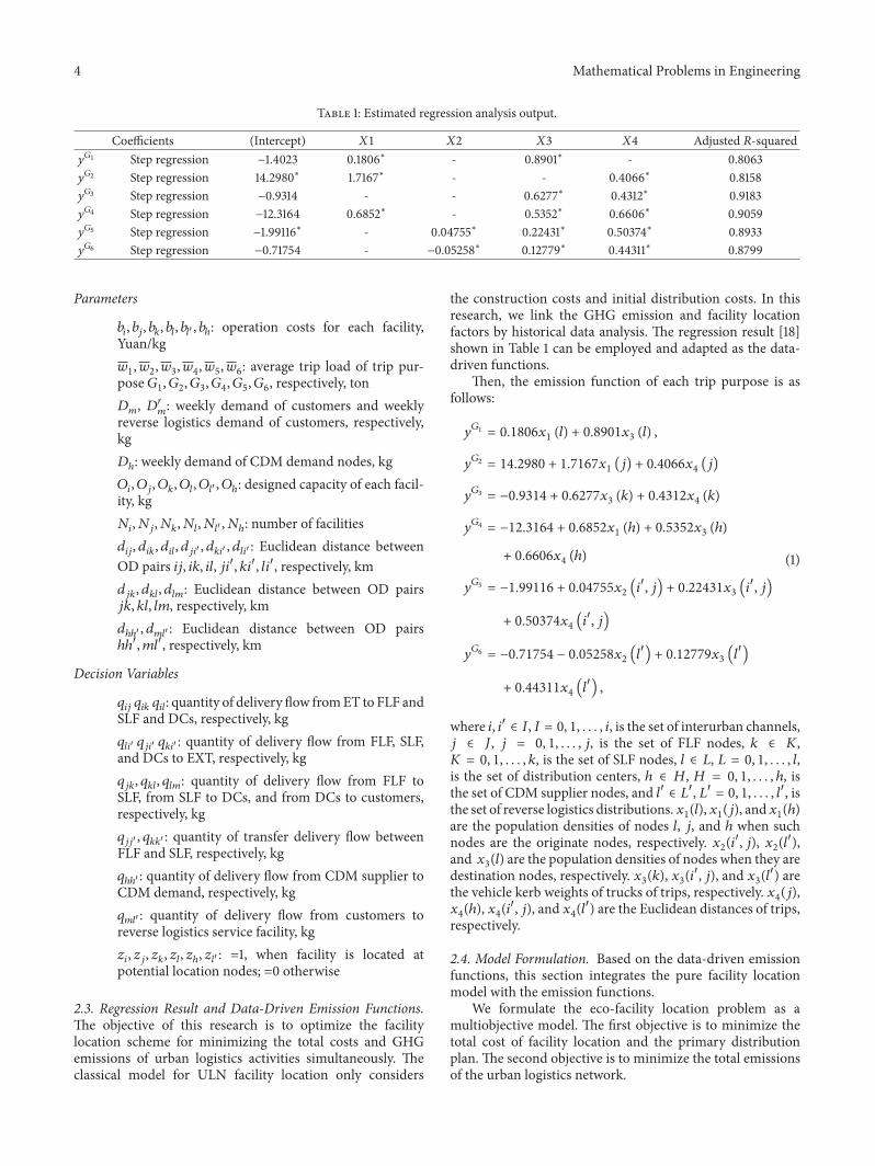
23 Regression Result and Data-Driven Emission FunctionsThe objective of this research is to optimize the facilitylocation scheme for minimizing the total costs and GHGemissions of urban logistics activities simultaneously Theclassical model for ULN facility location only considers
the construction costs and initial distribution costs In thisresearch we link the GHG emission and facility locationfactors by historical data analysis The regression result [18]shown in Table 1 can be employed and adapted as the data-driven functions
Then the emission function of each trip purpose is asfollows
1199101198666 = minus071754 minus 0052581199092 (1198971015840) + 0127791199093 (1198971015840)
+ 0443111199094 (1198971015840)
(1)
where 119894 1198941015840 isin 119868 119868 = 0 1 119894 is the set of interurban channels119895 isin 119869 119895 = 0 1 119895 is the set of FLF nodes 119896 isin 119870119870 = 0 1 119896 is the set of SLF nodes 119897 isin 119871 119871 = 0 1 119897is the set of distribution centers ℎ isin 119867 119867 = 0 1 ℎ isthe set of CDM supplier nodes and 1198971015840 isin 1198711015840 1198711015840 = 0 1 1198971015840 isthe set of reverse logistics distributions1199091(119897)1199091(119895) and1199091(ℎ)are the population densities of nodes 119897 119895 and ℎ when suchnodes are the originate nodes respectively 1199092(1198941015840 119895) 1199092(1198971015840)and 1199093(119897) are the population densities of nodes when they aredestination nodes respectively 1199093(119896) 1199093(1198941015840 119895) and 1199093(1198971015840) arethe vehicle kerb weights of trucks of trips respectively 1199094(119895)1199094(ℎ) 1199094(1198941015840 119895) and 1199094(1198971015840) are the Euclidean distances of tripsrespectively
24 Model Formulation Based on the data-driven emissionfunctions this section integrates the pure facility locationmodel with the emission functions
We formulate the eco-facility location problem as amultiobjective model The first objective is to minimize thetotal cost of facility location and the primary distributionplan The second objective is to minimize the total emissionsof the urban logistics network
Mathematical Problems in Engineering 5
The objective function is composed of delivery costsfacility construction costs and the total facilities operationcosts
The second objective is to minimize the total GHGemissions However the estimation functions can only rep-resent the GHG emissions of each single trip We thereforeintroduce trip1198661 trip1198662 trip1198663 trip1198664 trip1198665 and trip1198666 tostand for number of trips of each trip purpose respectivelyThen the relationship between trip count and flow quantitycan be explained as follows
The constraints are defined as follows (5) (6) and (7)guarantee that all the customer demands all the reverselogistics demands and theCDMdemands are served (8)ndash(11)are the flow equilibrium constraints (12)ndash(14) are the rela-tionship between location variables flow variables are con-fined by constraints (15)ndash(17) which also guarantee that thefacility designed capacity cannot be exceeded Equation (18)limits the facilities numbers Equation (19) is the nonnegativerestriction Equation (20) is the binary restriction
25 Solution Algorithms The data-driven function-basedfacility location model is a biobjective mixed-integer pro-gramming problem If we just take objective (4) and con-straints (5)ndash(11) and (19) into account the model is apure integer program problem However objective (2) and
Mathematical Problems in Engineering 7
constraints (12)ndash(18) and (20) are involved with fixed costsand binary variable increasing the complexity of the solvingapproach For the small-scaleULNproblemwe employed thelexicographic optimization based on the multistage simplexalgorithm to solve the model For the large-scale ULNproblem the heuristic algorithm or intelligent algorithms aresuitable for solving the problem
The approaches are as follows
Step 0 Establish the initial model including the two objec-tives ideal objective and realistic goal
Ideal Objective Objectives (2) and (4)
Realistic Goal
119891 (119886 119887 119902 119888 119911) = 0
sum119910 (G119899) times trip119866119899 = 0(21)
Step 1 Identify the expected value of each ideal objectivefunction introduce 120578119894 and 120588119894 as the negative deviationvariable and the positive deviation variable (resp) to realisticgoals and constraints 119894 is number of constraints and 120578119894 120588119894 ge 0to change the ideal objective function into realistic objectivefunction
Step 2 According to the goal deviation factors set in Step1 adding corresponding variables to the realistic objectivefunction and each constraint we change the model intoobjective programming
Step 3 Based on the proper degree of objectives we apply thelexicographic optimization technique technique to obtain thesingle objective standard lexicographic function In the prob-lem constraints (5)ndash(9) are hard constraints and the properdegree is first degree The proper degree of other constraintsis second degree The single objective lexicographic functionis
Step 4The abovemodel is also amixed-integer programmingproblem Since the problem scale is increased by addingvariables we employ the Particle Swarm Optimization algo-rithm and apply the PSO toolbox developed by George Evers[19] with Matlab R2015b to solve the model PSO algorithmfirst proposed by Eberhart and Kennedy [20] an optimalalgorithm based on the social behavior of bird flockinghas recently proven its high effectiveness and robustness insolving multiobjective problems
3 Numerical Experiments and Analysis
In this section we conduct the numerical experiments for theaforementioned model and algorithms The data we appliedare real data collected in Shenzhen city in the year 2011contemporaneous with the truck trajectory data
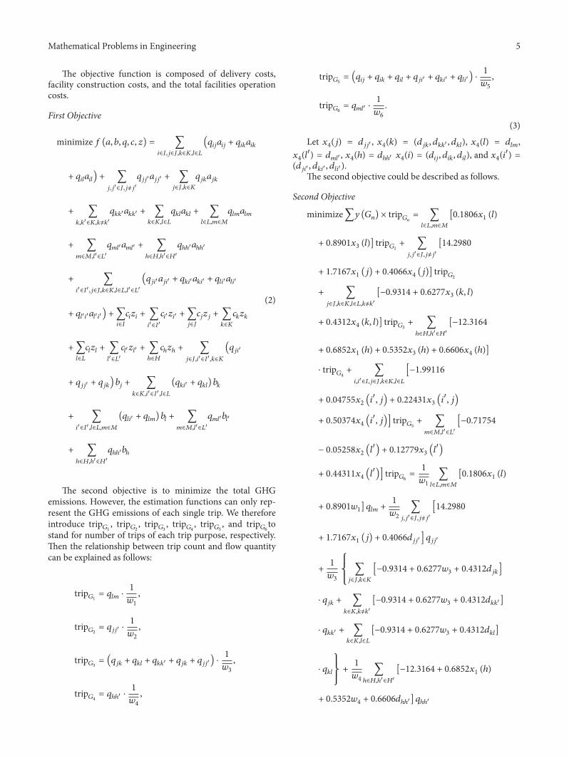
31 Numerical Experiments Description The logistics net-work of Shenzhen comprises fourth-echelon network fromthe first-degree logistics centers to final customers Thelocations of the first-degree logistics facilities are airports themain railway station the north railway station the Qianhaiports and Yantian ports which are numbered from 1 to 5Similarly the logistics parks (LP) are Jinpeng LP Yantianports LPQianhai Ports LP Songgang LPAirport LP LonghuaLP and Pinghu LP with corresponding numbers from 1 to 7 asthe second-degree logistics facilities The third-degree facil-ities mainly include distribution service centers (DSCs) Inour experiments we group the 460DCs into 10 accumulationareas to simplify the networkThe commercial and residentialareas are preprocessed into 12 zones in accordance with citymain center and secondary centers The highway tunnels ofenter and exit town of Shenzhen city are clustered into 5maincorridors by directionThemain supplier of CDM is groupedto 4 nodes so does the CDM demand nodes Figure 2 showsthe DCs location demand zones potential reverse logisticsfacility location and population density distribution of eachdistrict of Shenzhen city
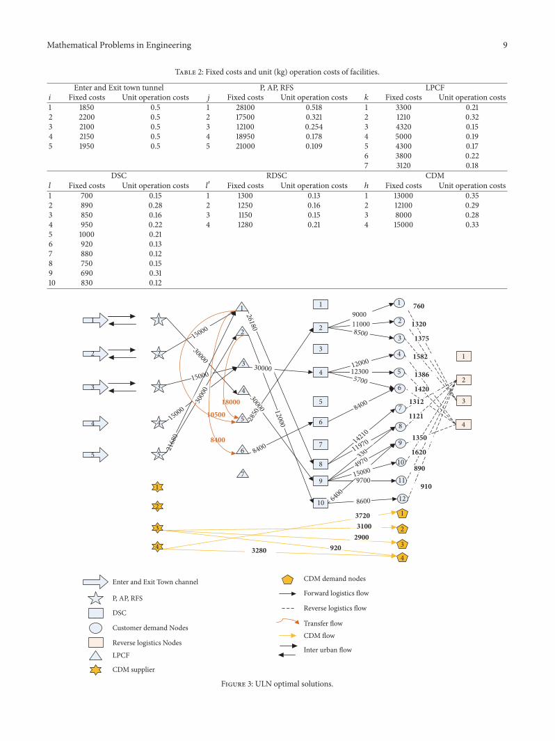
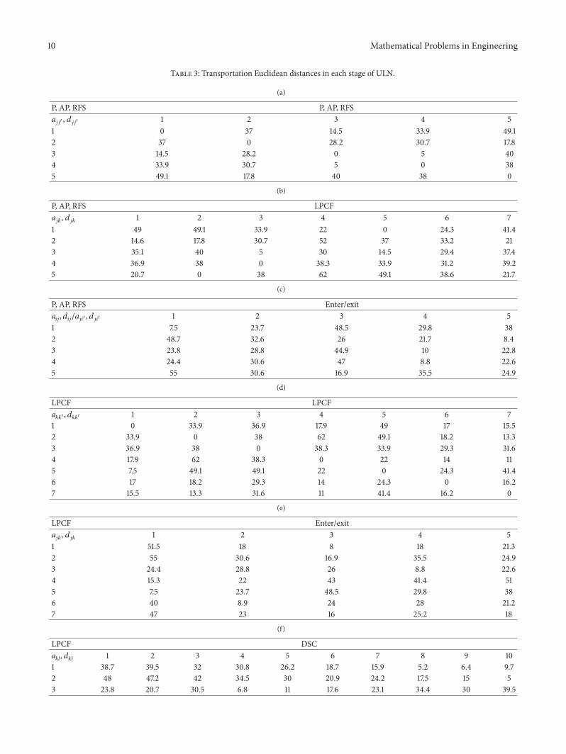
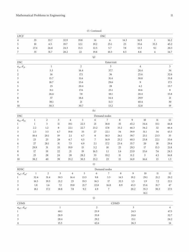
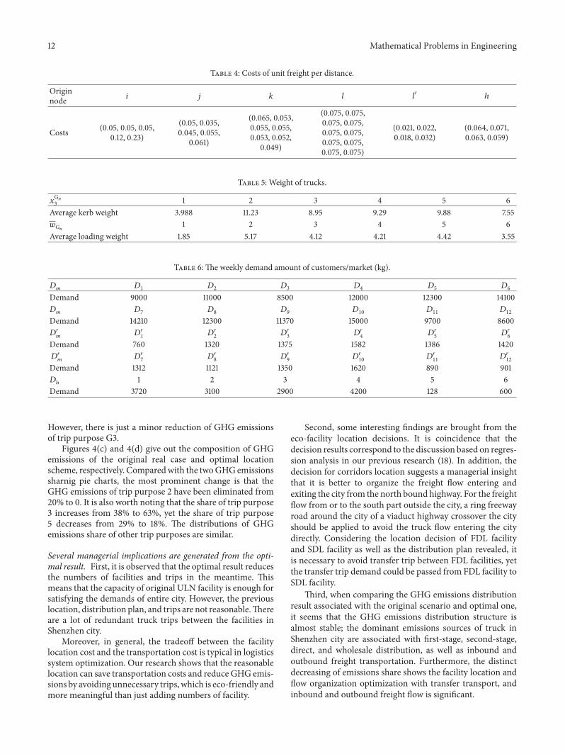
The capacity limit of first-degree facilities 1 2 and 3 allof the second-degree facilities and the DCs is 30000 kg Thecapacity limit of the harbor ports such as first-degree facilities4 and 5 is unlimited The capacity limit to CDM supplierand RL facility is 4000 kg The rest of related parametersare presented in Tables 2 3 4 and 5 Table 2 gives theweekly depreciation charge of construction fixed costs andunit operation costs of each facility Table 3 describes theEuclidean distance in eachOD pair Table 4 shows themarketcargo transport costs per unit per Euclidean distance Theaverage vehicle net weight is obtained from the truck dataand is shown in Table 5 Table 6 presents the demand of finalcustomer and CDM demand node
32 Results The optimal goal is to minimize the total ULNcosts as well as the GHG emissions simultaneously withsatisfying the logistics demand of the whole city We inputthe data apply the proposed model utilize the PSO toolboxmerged in Matlab R2015b and conduct the experiments bya PC with Intel core i7 processor to solve the problem Thesolver iterations are 50 and the elapsed runtime secondsare 010 s As can be seen in Figure 3 the optimal resultsof corridors selection location of each tier facilities andprimary distribution plan are displayed
The result shows that the main corridors for enteringand exiting city should be tunnels 1 2 and 3 The LP 1 23 4 5 6 DCs 2 4 6 8 9 and 10 RL facilities 2 3 and4 and CDM suppliers 3 and 4 are the optimal locations ofULN The designed capacity of airport main railway stationnorth railway station and Qianhai ports is no less than30000 15000 15000 and 15000 respectively The Yantianports undertake the major parts of urban freight of whichcapacity is 51680 The capacity of LP 1 2 3 4 5 and 6 is45080 30000 30000 30000 28500 and 8400 respectivelyFor DCs 2 4 6 8 9 and 10 the corresponding capacity is28500 30000 8400 26180 30000 and 12000 respectivelyFor RL facilities 2 3 and 4 the corresponding capacity is5844 3455 and 5738 respectively For CDM supplier thecapacity of node 3 is 6920 and the capacity of node 4 is 7000The initial distribution plan is also demonstrated clearly inthe figureThe arrow and text show the plan and volumeThelogistics flow generally from upstream to downstream nodesin the network Particularly the transfer transportation existsin second-degree facility The distribution plan is 10500 fromLP1 to LP5 8400 from LP1 to LP6 and 18000 from LP2 toLP5
4 Discussion and Managerial Insights
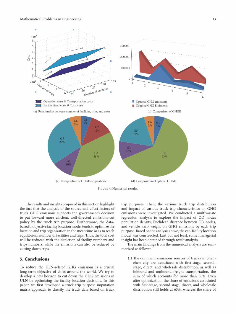
After optimization the total facilities of the city decrease from29 to 25 The number of truck trips of the city also decreasesfrom 90269 to 68117 Furthermore Figure 4(a) demonstratesthe relationship between number of facilities trips and costsThe arrow shows the increasing trend of various kinds of costsby trips and facilities
The comparison of GHG emissions rates (GHGE) of eachtrip purpose with original scenario against optimal scenariois displayed in Figure 4(b) The GHG emissions for trippurposes G1 G2 G4 G5 and G6 are reduced remarkably
Mathematical Problems in Engineering 9
Table 2 Fixed costs and unit (kg) operation costs of facilities
Enter and Exit town tunnel P AP RFS LPCF119894 Fixed costs Unit operation costs 119895 Fixed costs Unit operation costs 119896 Fixed costs Unit operation costs1 1850 05 1 28100 0518 1 3300 0212 2200 05 2 17500 0321 2 1210 0323 2100 05 3 12100 0254 3 4320 0154 2150 05 4 18950 0178 4 5000 0195 1950 05 5 21000 0109 5 4300 017
However there is just a minor reduction of GHG emissionsof trip purpose G3
Figures 4(c) and 4(d) give out the composition of GHGemissions of the original real case and optimal locationscheme respectively Comparedwith the twoGHGemissionssharnig pie charts the most prominent change is that theGHG emissions of trip purpose 2 have been eliminated from20 to 0 It is also worth noting that the share of trip purpose3 increases from 38 to 63 yet the share of trip purpose5 decreases from 29 to 18 The distributions of GHGemissions share of other trip purposes are similar
Several managerial implications are generated from the opti-mal result First it is observed that the optimal result reducesthe numbers of facilities and trips in the meantime Thismeans that the capacity of original ULN facility is enough forsatisfying the demands of entire city However the previouslocation distribution plan and trips are not reasonableThereare a lot of redundant truck trips between the facilities inShenzhen city
Moreover in general the tradeoff between the facilitylocation cost and the transportation cost is typical in logisticssystem optimization Our research shows that the reasonablelocation can save transportation costs and reduce GHG emis-sions by avoiding unnecessary trips which is eco-friendly andmore meaningful than just adding numbers of facility
Second some interesting findings are brought from theeco-facility location decisions It is coincidence that thedecision results correspond to the discussion based on regres-sion analysis in our previous research (18) In addition thedecision for corridors location suggests a managerial insightthat it is better to organize the freight flow entering andexiting the city from the north bound highway For the freightflow from or to the south part outside the city a ring freewayroad around the city of a viaduct highway crossover the cityshould be applied to avoid the truck flow entering the citydirectly Considering the location decision of FDL facilityand SDL facility as well as the distribution plan revealed itis necessary to avoid transfer trip between FDL facilities yetthe transfer trip demand could be passed from FDL facility toSDL facility
Third when comparing the GHG emissions distributionresult associated with the original scenario and optimal oneit seems that the GHG emissions distribution structure isalmost stable the dominant emissions sources of truck inShenzhen city are associated with first-stage second-stagedirect and wholesale distribution as well as inbound andoutbound freight transportation Furthermore the distinctdecreasing of emissions share shows the facility location andflow organization optimization with transfer transport andinbound and outbound freight flow is significant
Mathematical Problems in Engineering 13
25
26
27
28
29
Number of trips Number of facilities
Operation costs amp Transportation costsFacility fixed costs amp Total costs
10
9
8
7
6
6
5
4
3
2
1
0
Cos
t
times105
times104
(a) Relationship between number of facilities trips and costs
Optimal GHG emissionsOriginal GHG Emissions
300000
200000
100000
1
0
23
4
5
6
(b) Comparison of GHGE
G1
5G2
12
G3
38G4
10
G5
29
G6
6
(c) Composition of GHGE-original case
G1
5
G3
63
G4
10
G5
18
G6
5
(d) Composition of optimal GHGE
Figure 4 Numerical results
The results and insights proposed in this section highlightthe fact that the analysis of the source and effect factors oftruck GHG emissions supports the governmentrsquos decisionto put forward more efficient well-directed emissions-cutpolicy by the truck trip purpose Furthermore the data-based biobjective facility locationmodel tends to optimize thelocation and trip organization in the meantime so as to reachequilibrium number of facilities and tripsThus the total costwill be reduced with the depletion of facility numbers andtrips numbers while the emissions can also be reduced bycutting down trips
5 Conclusions
To reduce the ULN-related GHG emissions is a cruciallong-term objective of cities around the world We try todevelop a new horizon to cut down the GHG emissions inULN by optimizing the facility location decisions In thispaper we first developed a truck trip purpose imputationmatrix approach to classify the truck data based on truck
trip purposes Then the various truck trip distributionand impact of various truck trip characteristics on GHGemissions were investigated We conducted a multivariateregression analysis to explore the impact of OD nodespopulation density Euclidean distance between OD nodesand vehicle kerb weight on GHG emissions by each trippurpose Based on the analysis above the eco-facility locationmodel was constructed Last but not least some managerialinsight has been obtained through result analysis
The main findings from the numerical analysis are sum-marized as follows
(1) The dominant emissions sources of trucks in Shen-zhen city are associated with first-stage second-stage direct and wholesale distribution as well asinbound and outbound freight transportation thesum of which accounts for more than 60 Evenafter optimization the share of emissions associatedwith first-stage second-stage direct and wholesaledistribution still holds at 63 whereas the share of
14 Mathematical Problems in Engineering
emissions of inbound and outbound freight trans-portation reduced from 29 to 18
(2) There are a lot of redundant truck trips between thefacilities Reasonable locations can save transporta-tion costs and reduce GHG emissions by avoidingunnecessary trips which is eco-friendly and moremeaningful than just adding numbers of facility
(3) It is better to organize the freight flow entering andexiting the city from the north bound highway Forthe freight flow from or to the south part outside thecity a ring freeway road around the city of a viaducthighway crossover the city should be applied It isalso necessary to avoid transfer trip between first-degree logistics facilities such as airport railway andports yet the transfer trip demand could be passed tologistics parks
The above findings offer useful decision-support insightsto policy makers on efficient truck utilization ULN designand environment-friendly freight transport regulations Thefuture studymay include but will not be limited to usingmoredetailed trajectory data for emission estimation consideringland use type employment or establishment type and com-modity type as the independent variables and applying moresophisticated statistical tools in the analysis
Conflicts of Interest
The authors declare that there are no conflicts of interestregarding the publication of this paper
Acknowledgments
Thiswork is supported by theNational Natural Science Foun-dation of China (no 71403225 and no 60776827) the SoftScience Foundation of Sichuan Province (no 2014ZR0019)the Cyclic Economic Center of Sichuan Province (Projectno XHJJ-1411) the Soft science Foundation of Chengdu STA(Grant no 2015-RK00-00220-ZF) and Sichuan ProvincialSocial Sciences Foundation (Grant no SC16TJ031)
References
[1] EPA ldquoSource of Greenhouse gas emissionsrdquo httpswwwepagovclimatechangeghgemissionssourcestransportationGHGRP2013
[2] C Koc T Bektas O Jabali and G Laporte ldquoThe impact ofdepot location fleet composition and routing on emissions incity logisticsrdquo Transportation Research Part B Methodologicalvol 84 pp 81ndash102 2016
[3] M Gan S Chen and Y Yan ldquoThe effect of roadway capacityexpansion on facility sittingrdquo Applied Mathematics amp Informa-tion Sciences vol 7 no 2 L pp 575ndash581 2013
[4] H Hao Y Geng W Li and B Guo ldquoEnergy consumption andGHG emissions fromChinarsquos freight transport sector Scenariosthrough 2050rdquo Energy Policy vol 85 pp 94ndash101 2015
[5] J Sheu Y Chou and C Hu ldquoAn integrated logistics operationalmodel for green-supply chain managementrdquo Transportation
Research Part E Logistics and Transportation Review vol 41 no4 pp 287ndash313 2005
[6] K Boriboonsomsin M J Barth W Zhu and A Vu ldquoEco-routing navigation system based on multisource historical andreal-time traffic informationrdquo IEEE Transactions on IntelligentTransportation Systems vol 13 no 4 pp 1694ndash1704 2012
[7] KAhn andHARakha ldquoNetwork-wide impacts of eco-routingstrategies A large-scale case studyrdquo Transportation ResearchPart D Transport and Environment vol 25 pp 119ndash130 2013
[8] Y Nie and Q Li ldquoAn eco-routing model considering micro-scopic vehicle operating conditionsrdquo Transportation ResearchPart B Methodological vol 55 pp 154ndash170 2013
[9] G-H Tzeng ldquoMultiobjective Decision Making for TrafficAssignmentrdquo IEEE Transactions on Engineering Managementvol 40 no 2 pp 180ndash187 1993
[10] Y Yin and S Lawphongpanich ldquoInternalizing emission exter-nality on road networksrdquo Transportation Research Part DTransport and Environment vol 11 no 4 pp 292ndash301 2006
[11] W J Gutjahr and N Dzubur ldquoBi-objective bilevel optimizationof distribution center locations considering user equilibriardquoTransportation Research Part E Logistics and TransportationReview vol 85 pp 1ndash22 2016
[12] L Chen J Olhager and O Tang ldquoManufacturing facilitylocation and sustainability a literature review and researchagendardquo International Journal of Production Economics vol 149pp 154ndash163 2014
[13] C Ioannidou and J R OrsquoHanley ldquoEco-friendly location of smallhydropowerrdquo European Journal of Operational Research vol264 no 3 pp 907ndash918 2018
[14] F Wang X Lai and N Shi ldquoA multi-objective optimization forgreen supply chain network designrdquo Decision Support Systemsvol 51 no 2 pp 262ndash269 2011
[15] S Elhedhli and RMerrick ldquoGreen supply chain network designto reduce carbon emissionsrdquo Transportation Research Part DTransport and Environment vol 17 no 5 pp 370ndash379 2012
[16] Z He P Chen H Liu and Z Guo ldquoPerformance measurementsystem and strategies for developing low-carbon logistics a casestudy in Chinardquo Journal of Cleaner Production vol 156 pp 395ndash405 2017
[17] M S Pishvaee and J Razmi ldquoEnvironmental supply chainnetwork design using multi-objective fuzzy mathematical pro-grammingrdquo Applied Mathematical Modelling Simulation andComputation for Engineering and Environmental Systems vol36 no 8 pp 3433ndash3446 2012
[18] M Gan X Liu S Chen Y Yan and D Li ldquoThe identificationof truck-related greenhouse gas emissions and critical impactfactors in an urban logistics networkrdquo Journal of CleanerProduction vol 178 pp 561ndash571 2018
[19] ldquoPSO toolbox for matlabrdquo httpwwwgeorgeeversorgpsoresearch toolboxhtm
[20] R C Eberhart and J Kennedy ldquoParticle swarm optimizationinrdquo in Proceedings of IEEE International Conference on NeuralNetworks vol 4 p pp 1995
Hindawiwwwhindawicom Volume 2018
MathematicsJournal of
Hindawiwwwhindawicom Volume 2018
Mathematical Problems in Engineering
Applied MathematicsJournal of
Hindawiwwwhindawicom Volume 2018
Probability and StatisticsHindawiwwwhindawicom Volume 2018
Journal of
Hindawiwwwhindawicom Volume 2018
Mathematical PhysicsAdvances in
Complex AnalysisJournal of
Hindawiwwwhindawicom Volume 2018
OptimizationJournal of
Hindawiwwwhindawicom Volume 2018
Hindawiwwwhindawicom Volume 2018
Engineering Mathematics
International Journal of
Hindawiwwwhindawicom Volume 2018
Operations ResearchAdvances in
Journal of
Hindawiwwwhindawicom Volume 2018
Function SpacesAbstract and Applied AnalysisHindawiwwwhindawicom Volume 2018
International Journal of Mathematics and Mathematical Sciences
Numerical AnalysisNumerical AnalysisNumerical AnalysisNumerical AnalysisNumerical AnalysisNumerical AnalysisNumerical AnalysisNumerical AnalysisNumerical AnalysisNumerical AnalysisNumerical AnalysisNumerical AnalysisAdvances inAdvances in Discrete Dynamics in
Nature and SocietyHindawiwwwhindawicom Volume 2018
Hindawiwwwhindawicom
Dierential EquationsInternational Journal of
Volume 2018
Hindawiwwwhindawicom Volume 2018
Decision SciencesAdvances in
Hindawiwwwhindawicom Volume 2018
AnalysisInternational Journal of
Hindawiwwwhindawicom Volume 2018
Stochastic AnalysisInternational Journal of
Submit your manuscripts atwwwhindawicom
2 Mathematical Problems in Engineering
the construction and operation of facilities the running oftrucks and other freight carriers [2] Indeed the constructionand operation of the facility bring out a huge amount of GHGemissions due to the consumption of building materialsenergy and so forth The location of the facility is alsoinvolved with great deals of investment and will not beeasily relocated after the facility is constructed [3] For theaspect of truck-related GHG emissions trucks play a key rolein urban freight transport system and ULN [4] To reduceULN-related GHG emissions in cities various strategiesmay be considered to target to the aforementioned emissionsources With respect to the facility-emission sources sincethe relationship between emissions and inside activity of thefacility is not hard to estimate such as the electricity for runthe warehouse the diesel for forklift or package materialswe use in the warehouse it is obvious that minimizing thenumber and scale of facilities with satisfying the customerdemand as well as improving the energy efficiency can reducethe emissions [5] On the hand of reducing GHG emissionsof trucks the recent progress is mainly from the operationallevel [6] For instance we have the eco-routing problems andthe eco-traffic assignment problemThe former one is to findoptimal routes that promise tominimize fuel consumption orGHG emissions [7]The latter one is to incorporate the GHGemissions into the general traffic assignment models [8ndash10]However due to strict control regulations on truck trafficthe available truck routes in urban areas are often limitedonce the ULN design is fixed So it will be more efficient tooptimize the truck routes through the beginning the designstage of ULN rather than to optimize the truck routes afterthe important facility location is fixed (M Zhalechian et al2016) Then does the location of facility impact the GHGemission of ULN truck flow What is the interface betweenldquocharacteristics of locationrdquo and truck emissions The solu-tion of proposed questions may be used to relocate majorlogistics facilities which could potentially have far-reachingeffects in reducing long-term GHG emissions [11] Howeverthere is just limited knowledge about this field Aiming tofill such research gap we have investigated a large set ofempirical truck trajectory data developed a trip purposeimputation matrix to classify truck-related GHG emissionsand explored how the macroscopic trip would affect overallGHG emissions associated with each type of truck trips(X Liu and et al 2016) The mathematical relationshipsbetween GHG emissions and various kinds of trip purposespopulation density of origin nodesdestination nodes theEuclidean distance of each trip and vehicle kerb weightare captured through the multivariate regression analysisSome managerial insights are drawn from the findings yetthe mathematical representation of GHG emissions has notbeen applied to optimize the real logistics network in thecity
On the other hand the facility location problem as a hotissue in operations research has been investigated by numer-ous researchers and practitioners for centuries In additionthe location of logistics or supply chain facilities is an impor-tant composition With respect to the ECO facility locationproblem there are some related literatures about other kindsof facilities such as manufacturing facility and hydropower
location [12] For the logistics facility location problemconsidering carbon emissions Tang et al investigated thelogistics facility location model with consideration of eco-nomic costs services and CO2 emissions simultaneously[13] Wang et al formulated a multiobjective model for thesupply chain design problem in which the facility locationdecision is with environmental concerns [14] Elhedhli andMerrick modelled the relationship between emissions andvehicle weight and merged the emissions into the minimalcost objective by multiplying with the emissions cost [15]Some of other researchers also focus on traditional networkdesign with multiobjective and environmental aspects [1617] However the emissions rate is obtained by amacroscopicway Few of them explore the data-driven emissions functionthrough applying real truck trajectory data or consideringthe relationship between real truck trip emissions associatedwith various kinds of facilitiesWithwitness of above analysiswe attempted to propose a hypothesis that reasonable facilitylocation is able to reduce truck-related GHG emissionsFirst a group of GHG emissions functions by truck trip isdeveloped through analyzing the regressions results proposedin [18]Thenwe integrated theGHGemissions functions intothe logistics network design problem Similar to the modelstructure proposed by Wang et al [14] we constructed abiobjective eco-facility location model aiming to minimizethe total cost of facility location and truck-related GHGemissions simultaneously
The remainder of this paper is organized as followsThe data-driven emissions rate function the multiobjectivemodel and the solution algorithms are addressed in Sec-tion 2 In Section 3 we test the models and the algorithmsby real-case data Some managerial insights are drawn fromthe comparison and analysis of the results in Section 4 Theconclusion is given in Section 5
2 Models and Algorithms
21 Classification of Logistics Flow In our research since thetruck trip purpose is directly linked with diverse kinds offacilities first we describe the relationship of trip purposeand facility following with the trip purpose classificationin previous research [18] Figure 1 shows a typical logisticsnetwork The trucks are running as a freight carrier on thearcs linking diverse kinds of facilities or demand nodestogether
The truck trip purpose in a ULN could be classifiedinto 6 groups and 11 types The trip purposes are stronglyrelated to the properties of origin and destination nodes Suchrelationships are described as follows
Trip Purpose G1 Urban parcel distribution (PD) consists ofboth personnel parcel and electronic commerce distributionSale distribution (SD) usually stands for the situation wherethe seller delivers the goods to final customers Such trips arerelated to the third-degree logistics facility and communities(demand nodes)
Trip Purpose G2 Multimodal transfer trip (TT) refers to thegoods and cargoes that are transferred from one transport
Mathematical Problems in Engineering 3
Enter town channel
P AP RFS
Exit town channel
LPCF
First DegreeFacility
Second DegreeFacility
Third DegreeFacility Demand nodes
Inter-urban
Channel
Inter-urban
Channel
DSC Customer
CDM supplier
CDM demand nodes
demand nodes
Figure 1 A typical urban logistics network (note P AP and RFS refer to ports airports and freight railway stations resp DSC distributionservice center CDM chemistry and dangerous materials)
model freight station to another transport model freightstation Such trips are related to first-degree logistics (FDL)facility
Trip Purpose G3 First-stage distribution (FD) refers to bothforward and reverse distributions fromFDLnodes to second-degree logistics (SDL) nodes The second-stage distribution(SSD) stands for both forward and reverse distributions fromSDL nodes to third-level logistics nodes In particular thedistribution flow is from the first-level logistics nodes to thirdlevel sometimes which is represented as direct distribution(DD) Wholesale distribution (WD) represents the supplierdelivering goods to supermarketother retailers Such tripsare related to trips among first- second- and third-degreelogistics facilities
Trip Purpose G4 To meet the economic and social demandthe chemistry and dangerous materials transport in city areinevitable which is represented as CDMT Such trips arerelated to CDM supplier and demand nodes
Trip Purpose G5 In urban logistics it is common to seethe cargo flow from outside the urban boundaries andexit the urban boundaries We utilize inbound freight (IF)and outbound freight (OF) to describe the two scenariosrespectively Such trips are related to interurban corridors
Trip Purpose G6 RL refers to the residual reverse logisticsflow that has not been defined above Such trips are relatedto reverse logistics distribution centers and communities(demand nodes)
Then we formulate the eco-facility location model byintegrating the pure facility location model and truck tripGHG emissions function
22 Notations The notations to be used are listed as follows
Regression Variables
1199101198661 GHG emissions rate for single trip by trippurpose PD and SD
1199101198662 GHG emissions rate for single trip by trippurpose TT
1199101198663 GHG emissions rate for single trip by trippurpose FD SSD DD and WD
1199101198664 GHG emissions rate for single trip by trippurpose CDMT
1199101198665 GHG emissions rate for single trip by trippurpose IF and OF
1199101198666 GHG emissions rate for single trip by trippurpose RL
1198831 the population density of trip origin node
1198832 the population density of trip destination node
1198833 Vehicle kerb weight of trucks1198834 Euclidean distance between OD nodes of trucktrips
119887119894 119887119895 119887119896 119887119897 1198871198971015840 119887ℎ operation costs for each facilityYuankg1199081 1199082 1199083 1199084 1199085 1199086 average trip load of trip pur-pose 1198661 1198662 1198663 1198664 1198665 1198666 respectively ton119863119898 119863119903119898 weekly demand of customers and weeklyreverse logistics demand of customers respectivelykg119863ℎ weekly demand of CDM demand nodes kg119874119894 119874119895 119874119896 119874119897 1198741198971015840 119874ℎ designed capacity of each facil-ity kg119873119894 119873119895 119873119896 119873119897 1198731198971015840 119873ℎ number of facilities119889119894119895 119889119894119896 119889119894119897 1198891198951198941015840 1198891198961198941015840 1198891198971198941015840 Euclidean distance betweenOD pairs 119894119895 119894119896 119894119897 1198951198941015840 1198961198941015840 1198971198941015840 respectively km119889119895119896 119889119896119897 119889119897119898 Euclidean distance between OD pairs119895119896 119896119897 119897119898 respectively km119889ℎℎ1015840 1198891198981198971015840 Euclidean distance between OD pairsℎℎ1015840 1198981198971015840 respectively km
Decision Variables
119902119894119895 119902119894119896 119902119894119897 quantity of delivery flow fromET to FLF andSLF and DCs respectively kg1199021198971198941015840 1199021198951198941015840 1199021198961198941015840 quantity of delivery flow from FLF SLFand DCs to EXT respectively kg119902119895119896 119902119896119897 119902119897119898 quantity of delivery flow from FLF toSLF from SLF to DCs and from DCs to customersrespectively kg1199021198951198951015840 1199021198961198961015840 quantity of transfer delivery flow betweenFLF and SLF respectively kg119902ℎℎ1015840 quantity of delivery flow from CDM supplier toCDM demand respectively kg1199021198981198971015840 quantity of delivery flow from customers toreverse logistics service facility kg119911119894 119911119895 119911119896 119911119897 119911ℎ 1199111198971015840 =1 when facility is located atpotential location nodes =0 otherwise
23 Regression Result and Data-Driven Emission FunctionsThe objective of this research is to optimize the facilitylocation scheme for minimizing the total costs and GHGemissions of urban logistics activities simultaneously Theclassical model for ULN facility location only considers
the construction costs and initial distribution costs In thisresearch we link the GHG emission and facility locationfactors by historical data analysis The regression result [18]shown in Table 1 can be employed and adapted as the data-driven functions
Then the emission function of each trip purpose is asfollows
1199101198666 = minus071754 minus 0052581199092 (1198971015840) + 0127791199093 (1198971015840)
+ 0443111199094 (1198971015840)
(1)
where 119894 1198941015840 isin 119868 119868 = 0 1 119894 is the set of interurban channels119895 isin 119869 119895 = 0 1 119895 is the set of FLF nodes 119896 isin 119870119870 = 0 1 119896 is the set of SLF nodes 119897 isin 119871 119871 = 0 1 119897is the set of distribution centers ℎ isin 119867 119867 = 0 1 ℎ isthe set of CDM supplier nodes and 1198971015840 isin 1198711015840 1198711015840 = 0 1 1198971015840 isthe set of reverse logistics distributions1199091(119897)1199091(119895) and1199091(ℎ)are the population densities of nodes 119897 119895 and ℎ when suchnodes are the originate nodes respectively 1199092(1198941015840 119895) 1199092(1198971015840)and 1199093(119897) are the population densities of nodes when they aredestination nodes respectively 1199093(119896) 1199093(1198941015840 119895) and 1199093(1198971015840) arethe vehicle kerb weights of trucks of trips respectively 1199094(119895)1199094(ℎ) 1199094(1198941015840 119895) and 1199094(1198971015840) are the Euclidean distances of tripsrespectively
24 Model Formulation Based on the data-driven emissionfunctions this section integrates the pure facility locationmodel with the emission functions
We formulate the eco-facility location problem as amultiobjective model The first objective is to minimize thetotal cost of facility location and the primary distributionplan The second objective is to minimize the total emissionsof the urban logistics network
Mathematical Problems in Engineering 5
The objective function is composed of delivery costsfacility construction costs and the total facilities operationcosts
The second objective is to minimize the total GHGemissions However the estimation functions can only rep-resent the GHG emissions of each single trip We thereforeintroduce trip1198661 trip1198662 trip1198663 trip1198664 trip1198665 and trip1198666 tostand for number of trips of each trip purpose respectivelyThen the relationship between trip count and flow quantitycan be explained as follows
The constraints are defined as follows (5) (6) and (7)guarantee that all the customer demands all the reverselogistics demands and theCDMdemands are served (8)ndash(11)are the flow equilibrium constraints (12)ndash(14) are the rela-tionship between location variables flow variables are con-fined by constraints (15)ndash(17) which also guarantee that thefacility designed capacity cannot be exceeded Equation (18)limits the facilities numbers Equation (19) is the nonnegativerestriction Equation (20) is the binary restriction
25 Solution Algorithms The data-driven function-basedfacility location model is a biobjective mixed-integer pro-gramming problem If we just take objective (4) and con-straints (5)ndash(11) and (19) into account the model is apure integer program problem However objective (2) and
Mathematical Problems in Engineering 7
constraints (12)ndash(18) and (20) are involved with fixed costsand binary variable increasing the complexity of the solvingapproach For the small-scaleULNproblemwe employed thelexicographic optimization based on the multistage simplexalgorithm to solve the model For the large-scale ULNproblem the heuristic algorithm or intelligent algorithms aresuitable for solving the problem
The approaches are as follows
Step 0 Establish the initial model including the two objec-tives ideal objective and realistic goal
Ideal Objective Objectives (2) and (4)
Realistic Goal
119891 (119886 119887 119902 119888 119911) = 0
sum119910 (G119899) times trip119866119899 = 0(21)
Step 1 Identify the expected value of each ideal objectivefunction introduce 120578119894 and 120588119894 as the negative deviationvariable and the positive deviation variable (resp) to realisticgoals and constraints 119894 is number of constraints and 120578119894 120588119894 ge 0to change the ideal objective function into realistic objectivefunction
Step 2 According to the goal deviation factors set in Step1 adding corresponding variables to the realistic objectivefunction and each constraint we change the model intoobjective programming
Step 3 Based on the proper degree of objectives we apply thelexicographic optimization technique technique to obtain thesingle objective standard lexicographic function In the prob-lem constraints (5)ndash(9) are hard constraints and the properdegree is first degree The proper degree of other constraintsis second degree The single objective lexicographic functionis
Step 4The abovemodel is also amixed-integer programmingproblem Since the problem scale is increased by addingvariables we employ the Particle Swarm Optimization algo-rithm and apply the PSO toolbox developed by George Evers[19] with Matlab R2015b to solve the model PSO algorithmfirst proposed by Eberhart and Kennedy [20] an optimalalgorithm based on the social behavior of bird flockinghas recently proven its high effectiveness and robustness insolving multiobjective problems
3 Numerical Experiments and Analysis
In this section we conduct the numerical experiments for theaforementioned model and algorithms The data we appliedare real data collected in Shenzhen city in the year 2011contemporaneous with the truck trajectory data
31 Numerical Experiments Description The logistics net-work of Shenzhen comprises fourth-echelon network fromthe first-degree logistics centers to final customers Thelocations of the first-degree logistics facilities are airports themain railway station the north railway station the Qianhaiports and Yantian ports which are numbered from 1 to 5Similarly the logistics parks (LP) are Jinpeng LP Yantianports LPQianhai Ports LP Songgang LPAirport LP LonghuaLP and Pinghu LP with corresponding numbers from 1 to 7 asthe second-degree logistics facilities The third-degree facil-ities mainly include distribution service centers (DSCs) Inour experiments we group the 460DCs into 10 accumulationareas to simplify the networkThe commercial and residentialareas are preprocessed into 12 zones in accordance with citymain center and secondary centers The highway tunnels ofenter and exit town of Shenzhen city are clustered into 5maincorridors by directionThemain supplier of CDM is groupedto 4 nodes so does the CDM demand nodes Figure 2 showsthe DCs location demand zones potential reverse logisticsfacility location and population density distribution of eachdistrict of Shenzhen city
The capacity limit of first-degree facilities 1 2 and 3 allof the second-degree facilities and the DCs is 30000 kg Thecapacity limit of the harbor ports such as first-degree facilities4 and 5 is unlimited The capacity limit to CDM supplierand RL facility is 4000 kg The rest of related parametersare presented in Tables 2 3 4 and 5 Table 2 gives theweekly depreciation charge of construction fixed costs andunit operation costs of each facility Table 3 describes theEuclidean distance in eachOD pair Table 4 shows themarketcargo transport costs per unit per Euclidean distance Theaverage vehicle net weight is obtained from the truck dataand is shown in Table 5 Table 6 presents the demand of finalcustomer and CDM demand node
32 Results The optimal goal is to minimize the total ULNcosts as well as the GHG emissions simultaneously withsatisfying the logistics demand of the whole city We inputthe data apply the proposed model utilize the PSO toolboxmerged in Matlab R2015b and conduct the experiments bya PC with Intel core i7 processor to solve the problem Thesolver iterations are 50 and the elapsed runtime secondsare 010 s As can be seen in Figure 3 the optimal resultsof corridors selection location of each tier facilities andprimary distribution plan are displayed
The result shows that the main corridors for enteringand exiting city should be tunnels 1 2 and 3 The LP 1 23 4 5 6 DCs 2 4 6 8 9 and 10 RL facilities 2 3 and4 and CDM suppliers 3 and 4 are the optimal locations ofULN The designed capacity of airport main railway stationnorth railway station and Qianhai ports is no less than30000 15000 15000 and 15000 respectively The Yantianports undertake the major parts of urban freight of whichcapacity is 51680 The capacity of LP 1 2 3 4 5 and 6 is45080 30000 30000 30000 28500 and 8400 respectivelyFor DCs 2 4 6 8 9 and 10 the corresponding capacity is28500 30000 8400 26180 30000 and 12000 respectivelyFor RL facilities 2 3 and 4 the corresponding capacity is5844 3455 and 5738 respectively For CDM supplier thecapacity of node 3 is 6920 and the capacity of node 4 is 7000The initial distribution plan is also demonstrated clearly inthe figureThe arrow and text show the plan and volumeThelogistics flow generally from upstream to downstream nodesin the network Particularly the transfer transportation existsin second-degree facility The distribution plan is 10500 fromLP1 to LP5 8400 from LP1 to LP6 and 18000 from LP2 toLP5
4 Discussion and Managerial Insights
After optimization the total facilities of the city decrease from29 to 25 The number of truck trips of the city also decreasesfrom 90269 to 68117 Furthermore Figure 4(a) demonstratesthe relationship between number of facilities trips and costsThe arrow shows the increasing trend of various kinds of costsby trips and facilities
The comparison of GHG emissions rates (GHGE) of eachtrip purpose with original scenario against optimal scenariois displayed in Figure 4(b) The GHG emissions for trippurposes G1 G2 G4 G5 and G6 are reduced remarkably
Mathematical Problems in Engineering 9
Table 2 Fixed costs and unit (kg) operation costs of facilities
Enter and Exit town tunnel P AP RFS LPCF119894 Fixed costs Unit operation costs 119895 Fixed costs Unit operation costs 119896 Fixed costs Unit operation costs1 1850 05 1 28100 0518 1 3300 0212 2200 05 2 17500 0321 2 1210 0323 2100 05 3 12100 0254 3 4320 0154 2150 05 4 18950 0178 4 5000 0195 1950 05 5 21000 0109 5 4300 017
However there is just a minor reduction of GHG emissionsof trip purpose G3
Figures 4(c) and 4(d) give out the composition of GHGemissions of the original real case and optimal locationscheme respectively Comparedwith the twoGHGemissionssharnig pie charts the most prominent change is that theGHG emissions of trip purpose 2 have been eliminated from20 to 0 It is also worth noting that the share of trip purpose3 increases from 38 to 63 yet the share of trip purpose5 decreases from 29 to 18 The distributions of GHGemissions share of other trip purposes are similar
Several managerial implications are generated from the opti-mal result First it is observed that the optimal result reducesthe numbers of facilities and trips in the meantime Thismeans that the capacity of original ULN facility is enough forsatisfying the demands of entire city However the previouslocation distribution plan and trips are not reasonableThereare a lot of redundant truck trips between the facilities inShenzhen city
Moreover in general the tradeoff between the facilitylocation cost and the transportation cost is typical in logisticssystem optimization Our research shows that the reasonablelocation can save transportation costs and reduce GHG emis-sions by avoiding unnecessary trips which is eco-friendly andmore meaningful than just adding numbers of facility
Second some interesting findings are brought from theeco-facility location decisions It is coincidence that thedecision results correspond to the discussion based on regres-sion analysis in our previous research (18) In addition thedecision for corridors location suggests a managerial insightthat it is better to organize the freight flow entering andexiting the city from the north bound highway For the freightflow from or to the south part outside the city a ring freewayroad around the city of a viaduct highway crossover the cityshould be applied to avoid the truck flow entering the citydirectly Considering the location decision of FDL facilityand SDL facility as well as the distribution plan revealed itis necessary to avoid transfer trip between FDL facilities yetthe transfer trip demand could be passed from FDL facility toSDL facility
Third when comparing the GHG emissions distributionresult associated with the original scenario and optimal oneit seems that the GHG emissions distribution structure isalmost stable the dominant emissions sources of truck inShenzhen city are associated with first-stage second-stagedirect and wholesale distribution as well as inbound andoutbound freight transportation Furthermore the distinctdecreasing of emissions share shows the facility location andflow organization optimization with transfer transport andinbound and outbound freight flow is significant
Mathematical Problems in Engineering 13
25
26
27
28
29
Number of trips Number of facilities
Operation costs amp Transportation costsFacility fixed costs amp Total costs
10
9
8
7
6
6
5
4
3
2
1
0
Cos
t
times105
times104
(a) Relationship between number of facilities trips and costs
Optimal GHG emissionsOriginal GHG Emissions
300000
200000
100000
1
0
23
4
5
6
(b) Comparison of GHGE
G1
5G2
12
G3
38G4
10
G5
29
G6
6
(c) Composition of GHGE-original case
G1
5
G3
63
G4
10
G5
18
G6
5
(d) Composition of optimal GHGE
Figure 4 Numerical results
The results and insights proposed in this section highlightthe fact that the analysis of the source and effect factors oftruck GHG emissions supports the governmentrsquos decisionto put forward more efficient well-directed emissions-cutpolicy by the truck trip purpose Furthermore the data-based biobjective facility locationmodel tends to optimize thelocation and trip organization in the meantime so as to reachequilibrium number of facilities and tripsThus the total costwill be reduced with the depletion of facility numbers andtrips numbers while the emissions can also be reduced bycutting down trips
5 Conclusions
To reduce the ULN-related GHG emissions is a cruciallong-term objective of cities around the world We try todevelop a new horizon to cut down the GHG emissions inULN by optimizing the facility location decisions In thispaper we first developed a truck trip purpose imputationmatrix approach to classify the truck data based on truck
trip purposes Then the various truck trip distributionand impact of various truck trip characteristics on GHGemissions were investigated We conducted a multivariateregression analysis to explore the impact of OD nodespopulation density Euclidean distance between OD nodesand vehicle kerb weight on GHG emissions by each trippurpose Based on the analysis above the eco-facility locationmodel was constructed Last but not least some managerialinsight has been obtained through result analysis
The main findings from the numerical analysis are sum-marized as follows
(1) The dominant emissions sources of trucks in Shen-zhen city are associated with first-stage second-stage direct and wholesale distribution as well asinbound and outbound freight transportation thesum of which accounts for more than 60 Evenafter optimization the share of emissions associatedwith first-stage second-stage direct and wholesaledistribution still holds at 63 whereas the share of
14 Mathematical Problems in Engineering
emissions of inbound and outbound freight trans-portation reduced from 29 to 18
(2) There are a lot of redundant truck trips between thefacilities Reasonable locations can save transporta-tion costs and reduce GHG emissions by avoidingunnecessary trips which is eco-friendly and moremeaningful than just adding numbers of facility
(3) It is better to organize the freight flow entering andexiting the city from the north bound highway Forthe freight flow from or to the south part outside thecity a ring freeway road around the city of a viaducthighway crossover the city should be applied It isalso necessary to avoid transfer trip between first-degree logistics facilities such as airport railway andports yet the transfer trip demand could be passed tologistics parks
The above findings offer useful decision-support insightsto policy makers on efficient truck utilization ULN designand environment-friendly freight transport regulations Thefuture studymay include but will not be limited to usingmoredetailed trajectory data for emission estimation consideringland use type employment or establishment type and com-modity type as the independent variables and applying moresophisticated statistical tools in the analysis
Conflicts of Interest
The authors declare that there are no conflicts of interestregarding the publication of this paper
Acknowledgments
Thiswork is supported by theNational Natural Science Foun-dation of China (no 71403225 and no 60776827) the SoftScience Foundation of Sichuan Province (no 2014ZR0019)the Cyclic Economic Center of Sichuan Province (Projectno XHJJ-1411) the Soft science Foundation of Chengdu STA(Grant no 2015-RK00-00220-ZF) and Sichuan ProvincialSocial Sciences Foundation (Grant no SC16TJ031)
References
[1] EPA ldquoSource of Greenhouse gas emissionsrdquo httpswwwepagovclimatechangeghgemissionssourcestransportationGHGRP2013
[2] C Koc T Bektas O Jabali and G Laporte ldquoThe impact ofdepot location fleet composition and routing on emissions incity logisticsrdquo Transportation Research Part B Methodologicalvol 84 pp 81ndash102 2016
[3] M Gan S Chen and Y Yan ldquoThe effect of roadway capacityexpansion on facility sittingrdquo Applied Mathematics amp Informa-tion Sciences vol 7 no 2 L pp 575ndash581 2013
[4] H Hao Y Geng W Li and B Guo ldquoEnergy consumption andGHG emissions fromChinarsquos freight transport sector Scenariosthrough 2050rdquo Energy Policy vol 85 pp 94ndash101 2015
[5] J Sheu Y Chou and C Hu ldquoAn integrated logistics operationalmodel for green-supply chain managementrdquo Transportation
Research Part E Logistics and Transportation Review vol 41 no4 pp 287ndash313 2005
[6] K Boriboonsomsin M J Barth W Zhu and A Vu ldquoEco-routing navigation system based on multisource historical andreal-time traffic informationrdquo IEEE Transactions on IntelligentTransportation Systems vol 13 no 4 pp 1694ndash1704 2012
[7] KAhn andHARakha ldquoNetwork-wide impacts of eco-routingstrategies A large-scale case studyrdquo Transportation ResearchPart D Transport and Environment vol 25 pp 119ndash130 2013
[8] Y Nie and Q Li ldquoAn eco-routing model considering micro-scopic vehicle operating conditionsrdquo Transportation ResearchPart B Methodological vol 55 pp 154ndash170 2013
[9] G-H Tzeng ldquoMultiobjective Decision Making for TrafficAssignmentrdquo IEEE Transactions on Engineering Managementvol 40 no 2 pp 180ndash187 1993
[10] Y Yin and S Lawphongpanich ldquoInternalizing emission exter-nality on road networksrdquo Transportation Research Part DTransport and Environment vol 11 no 4 pp 292ndash301 2006
[11] W J Gutjahr and N Dzubur ldquoBi-objective bilevel optimizationof distribution center locations considering user equilibriardquoTransportation Research Part E Logistics and TransportationReview vol 85 pp 1ndash22 2016
[12] L Chen J Olhager and O Tang ldquoManufacturing facilitylocation and sustainability a literature review and researchagendardquo International Journal of Production Economics vol 149pp 154ndash163 2014
[13] C Ioannidou and J R OrsquoHanley ldquoEco-friendly location of smallhydropowerrdquo European Journal of Operational Research vol264 no 3 pp 907ndash918 2018
[14] F Wang X Lai and N Shi ldquoA multi-objective optimization forgreen supply chain network designrdquo Decision Support Systemsvol 51 no 2 pp 262ndash269 2011
[15] S Elhedhli and RMerrick ldquoGreen supply chain network designto reduce carbon emissionsrdquo Transportation Research Part DTransport and Environment vol 17 no 5 pp 370ndash379 2012
[16] Z He P Chen H Liu and Z Guo ldquoPerformance measurementsystem and strategies for developing low-carbon logistics a casestudy in Chinardquo Journal of Cleaner Production vol 156 pp 395ndash405 2017
[17] M S Pishvaee and J Razmi ldquoEnvironmental supply chainnetwork design using multi-objective fuzzy mathematical pro-grammingrdquo Applied Mathematical Modelling Simulation andComputation for Engineering and Environmental Systems vol36 no 8 pp 3433ndash3446 2012
[18] M Gan X Liu S Chen Y Yan and D Li ldquoThe identificationof truck-related greenhouse gas emissions and critical impactfactors in an urban logistics networkrdquo Journal of CleanerProduction vol 178 pp 561ndash571 2018
[19] ldquoPSO toolbox for matlabrdquo httpwwwgeorgeeversorgpsoresearch toolboxhtm
[20] R C Eberhart and J Kennedy ldquoParticle swarm optimizationinrdquo in Proceedings of IEEE International Conference on NeuralNetworks vol 4 p pp 1995
Hindawiwwwhindawicom Volume 2018
MathematicsJournal of
Hindawiwwwhindawicom Volume 2018
Mathematical Problems in Engineering
Applied MathematicsJournal of
Hindawiwwwhindawicom Volume 2018
Probability and StatisticsHindawiwwwhindawicom Volume 2018
Journal of
Hindawiwwwhindawicom Volume 2018
Mathematical PhysicsAdvances in
Complex AnalysisJournal of
Hindawiwwwhindawicom Volume 2018
OptimizationJournal of
Hindawiwwwhindawicom Volume 2018
Hindawiwwwhindawicom Volume 2018
Engineering Mathematics
International Journal of
Hindawiwwwhindawicom Volume 2018
Operations ResearchAdvances in
Journal of
Hindawiwwwhindawicom Volume 2018
Function SpacesAbstract and Applied AnalysisHindawiwwwhindawicom Volume 2018
International Journal of Mathematics and Mathematical Sciences
Numerical AnalysisNumerical AnalysisNumerical AnalysisNumerical AnalysisNumerical AnalysisNumerical AnalysisNumerical AnalysisNumerical AnalysisNumerical AnalysisNumerical AnalysisNumerical AnalysisNumerical AnalysisAdvances inAdvances in Discrete Dynamics in
Nature and SocietyHindawiwwwhindawicom Volume 2018
Hindawiwwwhindawicom
Dierential EquationsInternational Journal of
Volume 2018
Hindawiwwwhindawicom Volume 2018
Decision SciencesAdvances in
Hindawiwwwhindawicom Volume 2018
AnalysisInternational Journal of
Hindawiwwwhindawicom Volume 2018
Stochastic AnalysisInternational Journal of
Submit your manuscripts atwwwhindawicom
Mathematical Problems in Engineering 3
Enter town channel
P AP RFS
Exit town channel
LPCF
First DegreeFacility
Second DegreeFacility
Third DegreeFacility Demand nodes
Inter-urban
Channel
Inter-urban
Channel
DSC Customer
CDM supplier
CDM demand nodes
demand nodes
Figure 1 A typical urban logistics network (note P AP and RFS refer to ports airports and freight railway stations resp DSC distributionservice center CDM chemistry and dangerous materials)
model freight station to another transport model freightstation Such trips are related to first-degree logistics (FDL)facility
Trip Purpose G3 First-stage distribution (FD) refers to bothforward and reverse distributions fromFDLnodes to second-degree logistics (SDL) nodes The second-stage distribution(SSD) stands for both forward and reverse distributions fromSDL nodes to third-level logistics nodes In particular thedistribution flow is from the first-level logistics nodes to thirdlevel sometimes which is represented as direct distribution(DD) Wholesale distribution (WD) represents the supplierdelivering goods to supermarketother retailers Such tripsare related to trips among first- second- and third-degreelogistics facilities
Trip Purpose G4 To meet the economic and social demandthe chemistry and dangerous materials transport in city areinevitable which is represented as CDMT Such trips arerelated to CDM supplier and demand nodes
Trip Purpose G5 In urban logistics it is common to seethe cargo flow from outside the urban boundaries andexit the urban boundaries We utilize inbound freight (IF)and outbound freight (OF) to describe the two scenariosrespectively Such trips are related to interurban corridors
Trip Purpose G6 RL refers to the residual reverse logisticsflow that has not been defined above Such trips are relatedto reverse logistics distribution centers and communities(demand nodes)
Then we formulate the eco-facility location model byintegrating the pure facility location model and truck tripGHG emissions function
22 Notations The notations to be used are listed as follows
Regression Variables
1199101198661 GHG emissions rate for single trip by trippurpose PD and SD
1199101198662 GHG emissions rate for single trip by trippurpose TT
1199101198663 GHG emissions rate for single trip by trippurpose FD SSD DD and WD
1199101198664 GHG emissions rate for single trip by trippurpose CDMT
1199101198665 GHG emissions rate for single trip by trippurpose IF and OF
1199101198666 GHG emissions rate for single trip by trippurpose RL
1198831 the population density of trip origin node
1198832 the population density of trip destination node
1198833 Vehicle kerb weight of trucks1198834 Euclidean distance between OD nodes of trucktrips
119887119894 119887119895 119887119896 119887119897 1198871198971015840 119887ℎ operation costs for each facilityYuankg1199081 1199082 1199083 1199084 1199085 1199086 average trip load of trip pur-pose 1198661 1198662 1198663 1198664 1198665 1198666 respectively ton119863119898 119863119903119898 weekly demand of customers and weeklyreverse logistics demand of customers respectivelykg119863ℎ weekly demand of CDM demand nodes kg119874119894 119874119895 119874119896 119874119897 1198741198971015840 119874ℎ designed capacity of each facil-ity kg119873119894 119873119895 119873119896 119873119897 1198731198971015840 119873ℎ number of facilities119889119894119895 119889119894119896 119889119894119897 1198891198951198941015840 1198891198961198941015840 1198891198971198941015840 Euclidean distance betweenOD pairs 119894119895 119894119896 119894119897 1198951198941015840 1198961198941015840 1198971198941015840 respectively km119889119895119896 119889119896119897 119889119897119898 Euclidean distance between OD pairs119895119896 119896119897 119897119898 respectively km119889ℎℎ1015840 1198891198981198971015840 Euclidean distance between OD pairsℎℎ1015840 1198981198971015840 respectively km
Decision Variables
119902119894119895 119902119894119896 119902119894119897 quantity of delivery flow fromET to FLF andSLF and DCs respectively kg1199021198971198941015840 1199021198951198941015840 1199021198961198941015840 quantity of delivery flow from FLF SLFand DCs to EXT respectively kg119902119895119896 119902119896119897 119902119897119898 quantity of delivery flow from FLF toSLF from SLF to DCs and from DCs to customersrespectively kg1199021198951198951015840 1199021198961198961015840 quantity of transfer delivery flow betweenFLF and SLF respectively kg119902ℎℎ1015840 quantity of delivery flow from CDM supplier toCDM demand respectively kg1199021198981198971015840 quantity of delivery flow from customers toreverse logistics service facility kg119911119894 119911119895 119911119896 119911119897 119911ℎ 1199111198971015840 =1 when facility is located atpotential location nodes =0 otherwise
23 Regression Result and Data-Driven Emission FunctionsThe objective of this research is to optimize the facilitylocation scheme for minimizing the total costs and GHGemissions of urban logistics activities simultaneously Theclassical model for ULN facility location only considers
the construction costs and initial distribution costs In thisresearch we link the GHG emission and facility locationfactors by historical data analysis The regression result [18]shown in Table 1 can be employed and adapted as the data-driven functions
Then the emission function of each trip purpose is asfollows
1199101198666 = minus071754 minus 0052581199092 (1198971015840) + 0127791199093 (1198971015840)
+ 0443111199094 (1198971015840)
(1)
where 119894 1198941015840 isin 119868 119868 = 0 1 119894 is the set of interurban channels119895 isin 119869 119895 = 0 1 119895 is the set of FLF nodes 119896 isin 119870119870 = 0 1 119896 is the set of SLF nodes 119897 isin 119871 119871 = 0 1 119897is the set of distribution centers ℎ isin 119867 119867 = 0 1 ℎ isthe set of CDM supplier nodes and 1198971015840 isin 1198711015840 1198711015840 = 0 1 1198971015840 isthe set of reverse logistics distributions1199091(119897)1199091(119895) and1199091(ℎ)are the population densities of nodes 119897 119895 and ℎ when suchnodes are the originate nodes respectively 1199092(1198941015840 119895) 1199092(1198971015840)and 1199093(119897) are the population densities of nodes when they aredestination nodes respectively 1199093(119896) 1199093(1198941015840 119895) and 1199093(1198971015840) arethe vehicle kerb weights of trucks of trips respectively 1199094(119895)1199094(ℎ) 1199094(1198941015840 119895) and 1199094(1198971015840) are the Euclidean distances of tripsrespectively
24 Model Formulation Based on the data-driven emissionfunctions this section integrates the pure facility locationmodel with the emission functions
We formulate the eco-facility location problem as amultiobjective model The first objective is to minimize thetotal cost of facility location and the primary distributionplan The second objective is to minimize the total emissionsof the urban logistics network
Mathematical Problems in Engineering 5
The objective function is composed of delivery costsfacility construction costs and the total facilities operationcosts
The second objective is to minimize the total GHGemissions However the estimation functions can only rep-resent the GHG emissions of each single trip We thereforeintroduce trip1198661 trip1198662 trip1198663 trip1198664 trip1198665 and trip1198666 tostand for number of trips of each trip purpose respectivelyThen the relationship between trip count and flow quantitycan be explained as follows
The constraints are defined as follows (5) (6) and (7)guarantee that all the customer demands all the reverselogistics demands and theCDMdemands are served (8)ndash(11)are the flow equilibrium constraints (12)ndash(14) are the rela-tionship between location variables flow variables are con-fined by constraints (15)ndash(17) which also guarantee that thefacility designed capacity cannot be exceeded Equation (18)limits the facilities numbers Equation (19) is the nonnegativerestriction Equation (20) is the binary restriction
25 Solution Algorithms The data-driven function-basedfacility location model is a biobjective mixed-integer pro-gramming problem If we just take objective (4) and con-straints (5)ndash(11) and (19) into account the model is apure integer program problem However objective (2) and
Mathematical Problems in Engineering 7
constraints (12)ndash(18) and (20) are involved with fixed costsand binary variable increasing the complexity of the solvingapproach For the small-scaleULNproblemwe employed thelexicographic optimization based on the multistage simplexalgorithm to solve the model For the large-scale ULNproblem the heuristic algorithm or intelligent algorithms aresuitable for solving the problem
The approaches are as follows
Step 0 Establish the initial model including the two objec-tives ideal objective and realistic goal
Ideal Objective Objectives (2) and (4)
Realistic Goal
119891 (119886 119887 119902 119888 119911) = 0
sum119910 (G119899) times trip119866119899 = 0(21)
Step 1 Identify the expected value of each ideal objectivefunction introduce 120578119894 and 120588119894 as the negative deviationvariable and the positive deviation variable (resp) to realisticgoals and constraints 119894 is number of constraints and 120578119894 120588119894 ge 0to change the ideal objective function into realistic objectivefunction
Step 2 According to the goal deviation factors set in Step1 adding corresponding variables to the realistic objectivefunction and each constraint we change the model intoobjective programming
Step 3 Based on the proper degree of objectives we apply thelexicographic optimization technique technique to obtain thesingle objective standard lexicographic function In the prob-lem constraints (5)ndash(9) are hard constraints and the properdegree is first degree The proper degree of other constraintsis second degree The single objective lexicographic functionis
Step 4The abovemodel is also amixed-integer programmingproblem Since the problem scale is increased by addingvariables we employ the Particle Swarm Optimization algo-rithm and apply the PSO toolbox developed by George Evers[19] with Matlab R2015b to solve the model PSO algorithmfirst proposed by Eberhart and Kennedy [20] an optimalalgorithm based on the social behavior of bird flockinghas recently proven its high effectiveness and robustness insolving multiobjective problems
3 Numerical Experiments and Analysis
In this section we conduct the numerical experiments for theaforementioned model and algorithms The data we appliedare real data collected in Shenzhen city in the year 2011contemporaneous with the truck trajectory data
31 Numerical Experiments Description The logistics net-work of Shenzhen comprises fourth-echelon network fromthe first-degree logistics centers to final customers Thelocations of the first-degree logistics facilities are airports themain railway station the north railway station the Qianhaiports and Yantian ports which are numbered from 1 to 5Similarly the logistics parks (LP) are Jinpeng LP Yantianports LPQianhai Ports LP Songgang LPAirport LP LonghuaLP and Pinghu LP with corresponding numbers from 1 to 7 asthe second-degree logistics facilities The third-degree facil-ities mainly include distribution service centers (DSCs) Inour experiments we group the 460DCs into 10 accumulationareas to simplify the networkThe commercial and residentialareas are preprocessed into 12 zones in accordance with citymain center and secondary centers The highway tunnels ofenter and exit town of Shenzhen city are clustered into 5maincorridors by directionThemain supplier of CDM is groupedto 4 nodes so does the CDM demand nodes Figure 2 showsthe DCs location demand zones potential reverse logisticsfacility location and population density distribution of eachdistrict of Shenzhen city
The capacity limit of first-degree facilities 1 2 and 3 allof the second-degree facilities and the DCs is 30000 kg Thecapacity limit of the harbor ports such as first-degree facilities4 and 5 is unlimited The capacity limit to CDM supplierand RL facility is 4000 kg The rest of related parametersare presented in Tables 2 3 4 and 5 Table 2 gives theweekly depreciation charge of construction fixed costs andunit operation costs of each facility Table 3 describes theEuclidean distance in eachOD pair Table 4 shows themarketcargo transport costs per unit per Euclidean distance Theaverage vehicle net weight is obtained from the truck dataand is shown in Table 5 Table 6 presents the demand of finalcustomer and CDM demand node
32 Results The optimal goal is to minimize the total ULNcosts as well as the GHG emissions simultaneously withsatisfying the logistics demand of the whole city We inputthe data apply the proposed model utilize the PSO toolboxmerged in Matlab R2015b and conduct the experiments bya PC with Intel core i7 processor to solve the problem Thesolver iterations are 50 and the elapsed runtime secondsare 010 s As can be seen in Figure 3 the optimal resultsof corridors selection location of each tier facilities andprimary distribution plan are displayed
The result shows that the main corridors for enteringand exiting city should be tunnels 1 2 and 3 The LP 1 23 4 5 6 DCs 2 4 6 8 9 and 10 RL facilities 2 3 and4 and CDM suppliers 3 and 4 are the optimal locations ofULN The designed capacity of airport main railway stationnorth railway station and Qianhai ports is no less than30000 15000 15000 and 15000 respectively The Yantianports undertake the major parts of urban freight of whichcapacity is 51680 The capacity of LP 1 2 3 4 5 and 6 is45080 30000 30000 30000 28500 and 8400 respectivelyFor DCs 2 4 6 8 9 and 10 the corresponding capacity is28500 30000 8400 26180 30000 and 12000 respectivelyFor RL facilities 2 3 and 4 the corresponding capacity is5844 3455 and 5738 respectively For CDM supplier thecapacity of node 3 is 6920 and the capacity of node 4 is 7000The initial distribution plan is also demonstrated clearly inthe figureThe arrow and text show the plan and volumeThelogistics flow generally from upstream to downstream nodesin the network Particularly the transfer transportation existsin second-degree facility The distribution plan is 10500 fromLP1 to LP5 8400 from LP1 to LP6 and 18000 from LP2 toLP5
4 Discussion and Managerial Insights
After optimization the total facilities of the city decrease from29 to 25 The number of truck trips of the city also decreasesfrom 90269 to 68117 Furthermore Figure 4(a) demonstratesthe relationship between number of facilities trips and costsThe arrow shows the increasing trend of various kinds of costsby trips and facilities
The comparison of GHG emissions rates (GHGE) of eachtrip purpose with original scenario against optimal scenariois displayed in Figure 4(b) The GHG emissions for trippurposes G1 G2 G4 G5 and G6 are reduced remarkably
Mathematical Problems in Engineering 9
Table 2 Fixed costs and unit (kg) operation costs of facilities
Enter and Exit town tunnel P AP RFS LPCF119894 Fixed costs Unit operation costs 119895 Fixed costs Unit operation costs 119896 Fixed costs Unit operation costs1 1850 05 1 28100 0518 1 3300 0212 2200 05 2 17500 0321 2 1210 0323 2100 05 3 12100 0254 3 4320 0154 2150 05 4 18950 0178 4 5000 0195 1950 05 5 21000 0109 5 4300 017
However there is just a minor reduction of GHG emissionsof trip purpose G3
Figures 4(c) and 4(d) give out the composition of GHGemissions of the original real case and optimal locationscheme respectively Comparedwith the twoGHGemissionssharnig pie charts the most prominent change is that theGHG emissions of trip purpose 2 have been eliminated from20 to 0 It is also worth noting that the share of trip purpose3 increases from 38 to 63 yet the share of trip purpose5 decreases from 29 to 18 The distributions of GHGemissions share of other trip purposes are similar
Several managerial implications are generated from the opti-mal result First it is observed that the optimal result reducesthe numbers of facilities and trips in the meantime Thismeans that the capacity of original ULN facility is enough forsatisfying the demands of entire city However the previouslocation distribution plan and trips are not reasonableThereare a lot of redundant truck trips between the facilities inShenzhen city
Moreover in general the tradeoff between the facilitylocation cost and the transportation cost is typical in logisticssystem optimization Our research shows that the reasonablelocation can save transportation costs and reduce GHG emis-sions by avoiding unnecessary trips which is eco-friendly andmore meaningful than just adding numbers of facility
Second some interesting findings are brought from theeco-facility location decisions It is coincidence that thedecision results correspond to the discussion based on regres-sion analysis in our previous research (18) In addition thedecision for corridors location suggests a managerial insightthat it is better to organize the freight flow entering andexiting the city from the north bound highway For the freightflow from or to the south part outside the city a ring freewayroad around the city of a viaduct highway crossover the cityshould be applied to avoid the truck flow entering the citydirectly Considering the location decision of FDL facilityand SDL facility as well as the distribution plan revealed itis necessary to avoid transfer trip between FDL facilities yetthe transfer trip demand could be passed from FDL facility toSDL facility
Third when comparing the GHG emissions distributionresult associated with the original scenario and optimal oneit seems that the GHG emissions distribution structure isalmost stable the dominant emissions sources of truck inShenzhen city are associated with first-stage second-stagedirect and wholesale distribution as well as inbound andoutbound freight transportation Furthermore the distinctdecreasing of emissions share shows the facility location andflow organization optimization with transfer transport andinbound and outbound freight flow is significant
Mathematical Problems in Engineering 13
25
26
27
28
29
Number of trips Number of facilities
Operation costs amp Transportation costsFacility fixed costs amp Total costs
10
9
8
7
6
6
5
4
3
2
1
0
Cos
t
times105
times104
(a) Relationship between number of facilities trips and costs
Optimal GHG emissionsOriginal GHG Emissions
300000
200000
100000
1
0
23
4
5
6
(b) Comparison of GHGE
G1
5G2
12
G3
38G4
10
G5
29
G6
6
(c) Composition of GHGE-original case
G1
5
G3
63
G4
10
G5
18
G6
5
(d) Composition of optimal GHGE
Figure 4 Numerical results
The results and insights proposed in this section highlightthe fact that the analysis of the source and effect factors oftruck GHG emissions supports the governmentrsquos decisionto put forward more efficient well-directed emissions-cutpolicy by the truck trip purpose Furthermore the data-based biobjective facility locationmodel tends to optimize thelocation and trip organization in the meantime so as to reachequilibrium number of facilities and tripsThus the total costwill be reduced with the depletion of facility numbers andtrips numbers while the emissions can also be reduced bycutting down trips
5 Conclusions
To reduce the ULN-related GHG emissions is a cruciallong-term objective of cities around the world We try todevelop a new horizon to cut down the GHG emissions inULN by optimizing the facility location decisions In thispaper we first developed a truck trip purpose imputationmatrix approach to classify the truck data based on truck
trip purposes Then the various truck trip distributionand impact of various truck trip characteristics on GHGemissions were investigated We conducted a multivariateregression analysis to explore the impact of OD nodespopulation density Euclidean distance between OD nodesand vehicle kerb weight on GHG emissions by each trippurpose Based on the analysis above the eco-facility locationmodel was constructed Last but not least some managerialinsight has been obtained through result analysis
The main findings from the numerical analysis are sum-marized as follows
(1) The dominant emissions sources of trucks in Shen-zhen city are associated with first-stage second-stage direct and wholesale distribution as well asinbound and outbound freight transportation thesum of which accounts for more than 60 Evenafter optimization the share of emissions associatedwith first-stage second-stage direct and wholesaledistribution still holds at 63 whereas the share of
14 Mathematical Problems in Engineering
emissions of inbound and outbound freight trans-portation reduced from 29 to 18
(2) There are a lot of redundant truck trips between thefacilities Reasonable locations can save transporta-tion costs and reduce GHG emissions by avoidingunnecessary trips which is eco-friendly and moremeaningful than just adding numbers of facility
(3) It is better to organize the freight flow entering andexiting the city from the north bound highway Forthe freight flow from or to the south part outside thecity a ring freeway road around the city of a viaducthighway crossover the city should be applied It isalso necessary to avoid transfer trip between first-degree logistics facilities such as airport railway andports yet the transfer trip demand could be passed tologistics parks
The above findings offer useful decision-support insightsto policy makers on efficient truck utilization ULN designand environment-friendly freight transport regulations Thefuture studymay include but will not be limited to usingmoredetailed trajectory data for emission estimation consideringland use type employment or establishment type and com-modity type as the independent variables and applying moresophisticated statistical tools in the analysis
Conflicts of Interest
The authors declare that there are no conflicts of interestregarding the publication of this paper
Acknowledgments
Thiswork is supported by theNational Natural Science Foun-dation of China (no 71403225 and no 60776827) the SoftScience Foundation of Sichuan Province (no 2014ZR0019)the Cyclic Economic Center of Sichuan Province (Projectno XHJJ-1411) the Soft science Foundation of Chengdu STA(Grant no 2015-RK00-00220-ZF) and Sichuan ProvincialSocial Sciences Foundation (Grant no SC16TJ031)
References
[1] EPA ldquoSource of Greenhouse gas emissionsrdquo httpswwwepagovclimatechangeghgemissionssourcestransportationGHGRP2013
[2] C Koc T Bektas O Jabali and G Laporte ldquoThe impact ofdepot location fleet composition and routing on emissions incity logisticsrdquo Transportation Research Part B Methodologicalvol 84 pp 81ndash102 2016
[3] M Gan S Chen and Y Yan ldquoThe effect of roadway capacityexpansion on facility sittingrdquo Applied Mathematics amp Informa-tion Sciences vol 7 no 2 L pp 575ndash581 2013
[4] H Hao Y Geng W Li and B Guo ldquoEnergy consumption andGHG emissions fromChinarsquos freight transport sector Scenariosthrough 2050rdquo Energy Policy vol 85 pp 94ndash101 2015
[5] J Sheu Y Chou and C Hu ldquoAn integrated logistics operationalmodel for green-supply chain managementrdquo Transportation
Research Part E Logistics and Transportation Review vol 41 no4 pp 287ndash313 2005
[6] K Boriboonsomsin M J Barth W Zhu and A Vu ldquoEco-routing navigation system based on multisource historical andreal-time traffic informationrdquo IEEE Transactions on IntelligentTransportation Systems vol 13 no 4 pp 1694ndash1704 2012
[7] KAhn andHARakha ldquoNetwork-wide impacts of eco-routingstrategies A large-scale case studyrdquo Transportation ResearchPart D Transport and Environment vol 25 pp 119ndash130 2013
[8] Y Nie and Q Li ldquoAn eco-routing model considering micro-scopic vehicle operating conditionsrdquo Transportation ResearchPart B Methodological vol 55 pp 154ndash170 2013
[9] G-H Tzeng ldquoMultiobjective Decision Making for TrafficAssignmentrdquo IEEE Transactions on Engineering Managementvol 40 no 2 pp 180ndash187 1993
[10] Y Yin and S Lawphongpanich ldquoInternalizing emission exter-nality on road networksrdquo Transportation Research Part DTransport and Environment vol 11 no 4 pp 292ndash301 2006
[11] W J Gutjahr and N Dzubur ldquoBi-objective bilevel optimizationof distribution center locations considering user equilibriardquoTransportation Research Part E Logistics and TransportationReview vol 85 pp 1ndash22 2016
[12] L Chen J Olhager and O Tang ldquoManufacturing facilitylocation and sustainability a literature review and researchagendardquo International Journal of Production Economics vol 149pp 154ndash163 2014
[13] C Ioannidou and J R OrsquoHanley ldquoEco-friendly location of smallhydropowerrdquo European Journal of Operational Research vol264 no 3 pp 907ndash918 2018
[14] F Wang X Lai and N Shi ldquoA multi-objective optimization forgreen supply chain network designrdquo Decision Support Systemsvol 51 no 2 pp 262ndash269 2011
[15] S Elhedhli and RMerrick ldquoGreen supply chain network designto reduce carbon emissionsrdquo Transportation Research Part DTransport and Environment vol 17 no 5 pp 370ndash379 2012
[16] Z He P Chen H Liu and Z Guo ldquoPerformance measurementsystem and strategies for developing low-carbon logistics a casestudy in Chinardquo Journal of Cleaner Production vol 156 pp 395ndash405 2017
[17] M S Pishvaee and J Razmi ldquoEnvironmental supply chainnetwork design using multi-objective fuzzy mathematical pro-grammingrdquo Applied Mathematical Modelling Simulation andComputation for Engineering and Environmental Systems vol36 no 8 pp 3433ndash3446 2012
[18] M Gan X Liu S Chen Y Yan and D Li ldquoThe identificationof truck-related greenhouse gas emissions and critical impactfactors in an urban logistics networkrdquo Journal of CleanerProduction vol 178 pp 561ndash571 2018
[19] ldquoPSO toolbox for matlabrdquo httpwwwgeorgeeversorgpsoresearch toolboxhtm
[20] R C Eberhart and J Kennedy ldquoParticle swarm optimizationinrdquo in Proceedings of IEEE International Conference on NeuralNetworks vol 4 p pp 1995
Hindawiwwwhindawicom Volume 2018
MathematicsJournal of
Hindawiwwwhindawicom Volume 2018
Mathematical Problems in Engineering
Applied MathematicsJournal of
Hindawiwwwhindawicom Volume 2018
Probability and StatisticsHindawiwwwhindawicom Volume 2018
Journal of
Hindawiwwwhindawicom Volume 2018
Mathematical PhysicsAdvances in
Complex AnalysisJournal of
Hindawiwwwhindawicom Volume 2018
OptimizationJournal of
Hindawiwwwhindawicom Volume 2018
Hindawiwwwhindawicom Volume 2018
Engineering Mathematics
International Journal of
Hindawiwwwhindawicom Volume 2018
Operations ResearchAdvances in
Journal of
Hindawiwwwhindawicom Volume 2018
Function SpacesAbstract and Applied AnalysisHindawiwwwhindawicom Volume 2018
International Journal of Mathematics and Mathematical Sciences
Numerical AnalysisNumerical AnalysisNumerical AnalysisNumerical AnalysisNumerical AnalysisNumerical AnalysisNumerical AnalysisNumerical AnalysisNumerical AnalysisNumerical AnalysisNumerical AnalysisNumerical AnalysisAdvances inAdvances in Discrete Dynamics in
Nature and SocietyHindawiwwwhindawicom Volume 2018
Hindawiwwwhindawicom
Dierential EquationsInternational Journal of
Volume 2018
Hindawiwwwhindawicom Volume 2018
Decision SciencesAdvances in
Hindawiwwwhindawicom Volume 2018
AnalysisInternational Journal of
Hindawiwwwhindawicom Volume 2018
Stochastic AnalysisInternational Journal of
Submit your manuscripts atwwwhindawicom
Mathematical Problems in Engineering 7
constraints (12)ndash(18) and (20) are involved with fixed costsand binary variable increasing the complexity of the solvingapproach For the small-scaleULNproblemwe employed thelexicographic optimization based on the multistage simplexalgorithm to solve the model For the large-scale ULNproblem the heuristic algorithm or intelligent algorithms aresuitable for solving the problem
The approaches are as follows
Step 0 Establish the initial model including the two objec-tives ideal objective and realistic goal
Ideal Objective Objectives (2) and (4)
Realistic Goal
119891 (119886 119887 119902 119888 119911) = 0
sum119910 (G119899) times trip119866119899 = 0(21)
Step 1 Identify the expected value of each ideal objectivefunction introduce 120578119894 and 120588119894 as the negative deviationvariable and the positive deviation variable (resp) to realisticgoals and constraints 119894 is number of constraints and 120578119894 120588119894 ge 0to change the ideal objective function into realistic objectivefunction
Step 2 According to the goal deviation factors set in Step1 adding corresponding variables to the realistic objectivefunction and each constraint we change the model intoobjective programming
Step 3 Based on the proper degree of objectives we apply thelexicographic optimization technique technique to obtain thesingle objective standard lexicographic function In the prob-lem constraints (5)ndash(9) are hard constraints and the properdegree is first degree The proper degree of other constraintsis second degree The single objective lexicographic functionis
Step 4The abovemodel is also amixed-integer programmingproblem Since the problem scale is increased by addingvariables we employ the Particle Swarm Optimization algo-rithm and apply the PSO toolbox developed by George Evers[19] with Matlab R2015b to solve the model PSO algorithmfirst proposed by Eberhart and Kennedy [20] an optimalalgorithm based on the social behavior of bird flockinghas recently proven its high effectiveness and robustness insolving multiobjective problems
3 Numerical Experiments and Analysis
In this section we conduct the numerical experiments for theaforementioned model and algorithms The data we appliedare real data collected in Shenzhen city in the year 2011contemporaneous with the truck trajectory data
31 Numerical Experiments Description The logistics net-work of Shenzhen comprises fourth-echelon network fromthe first-degree logistics centers to final customers Thelocations of the first-degree logistics facilities are airports themain railway station the north railway station the Qianhaiports and Yantian ports which are numbered from 1 to 5Similarly the logistics parks (LP) are Jinpeng LP Yantianports LPQianhai Ports LP Songgang LPAirport LP LonghuaLP and Pinghu LP with corresponding numbers from 1 to 7 asthe second-degree logistics facilities The third-degree facil-ities mainly include distribution service centers (DSCs) Inour experiments we group the 460DCs into 10 accumulationareas to simplify the networkThe commercial and residentialareas are preprocessed into 12 zones in accordance with citymain center and secondary centers The highway tunnels ofenter and exit town of Shenzhen city are clustered into 5maincorridors by directionThemain supplier of CDM is groupedto 4 nodes so does the CDM demand nodes Figure 2 showsthe DCs location demand zones potential reverse logisticsfacility location and population density distribution of eachdistrict of Shenzhen city
The capacity limit of first-degree facilities 1 2 and 3 allof the second-degree facilities and the DCs is 30000 kg Thecapacity limit of the harbor ports such as first-degree facilities4 and 5 is unlimited The capacity limit to CDM supplierand RL facility is 4000 kg The rest of related parametersare presented in Tables 2 3 4 and 5 Table 2 gives theweekly depreciation charge of construction fixed costs andunit operation costs of each facility Table 3 describes theEuclidean distance in eachOD pair Table 4 shows themarketcargo transport costs per unit per Euclidean distance Theaverage vehicle net weight is obtained from the truck dataand is shown in Table 5 Table 6 presents the demand of finalcustomer and CDM demand node
32 Results The optimal goal is to minimize the total ULNcosts as well as the GHG emissions simultaneously withsatisfying the logistics demand of the whole city We inputthe data apply the proposed model utilize the PSO toolboxmerged in Matlab R2015b and conduct the experiments bya PC with Intel core i7 processor to solve the problem Thesolver iterations are 50 and the elapsed runtime secondsare 010 s As can be seen in Figure 3 the optimal resultsof corridors selection location of each tier facilities andprimary distribution plan are displayed
The result shows that the main corridors for enteringand exiting city should be tunnels 1 2 and 3 The LP 1 23 4 5 6 DCs 2 4 6 8 9 and 10 RL facilities 2 3 and4 and CDM suppliers 3 and 4 are the optimal locations ofULN The designed capacity of airport main railway stationnorth railway station and Qianhai ports is no less than30000 15000 15000 and 15000 respectively The Yantianports undertake the major parts of urban freight of whichcapacity is 51680 The capacity of LP 1 2 3 4 5 and 6 is45080 30000 30000 30000 28500 and 8400 respectivelyFor DCs 2 4 6 8 9 and 10 the corresponding capacity is28500 30000 8400 26180 30000 and 12000 respectivelyFor RL facilities 2 3 and 4 the corresponding capacity is5844 3455 and 5738 respectively For CDM supplier thecapacity of node 3 is 6920 and the capacity of node 4 is 7000The initial distribution plan is also demonstrated clearly inthe figureThe arrow and text show the plan and volumeThelogistics flow generally from upstream to downstream nodesin the network Particularly the transfer transportation existsin second-degree facility The distribution plan is 10500 fromLP1 to LP5 8400 from LP1 to LP6 and 18000 from LP2 toLP5
4 Discussion and Managerial Insights
After optimization the total facilities of the city decrease from29 to 25 The number of truck trips of the city also decreasesfrom 90269 to 68117 Furthermore Figure 4(a) demonstratesthe relationship between number of facilities trips and costsThe arrow shows the increasing trend of various kinds of costsby trips and facilities
The comparison of GHG emissions rates (GHGE) of eachtrip purpose with original scenario against optimal scenariois displayed in Figure 4(b) The GHG emissions for trippurposes G1 G2 G4 G5 and G6 are reduced remarkably
Mathematical Problems in Engineering 9
Table 2 Fixed costs and unit (kg) operation costs of facilities
Enter and Exit town tunnel P AP RFS LPCF119894 Fixed costs Unit operation costs 119895 Fixed costs Unit operation costs 119896 Fixed costs Unit operation costs1 1850 05 1 28100 0518 1 3300 0212 2200 05 2 17500 0321 2 1210 0323 2100 05 3 12100 0254 3 4320 0154 2150 05 4 18950 0178 4 5000 0195 1950 05 5 21000 0109 5 4300 017
However there is just a minor reduction of GHG emissionsof trip purpose G3
Figures 4(c) and 4(d) give out the composition of GHGemissions of the original real case and optimal locationscheme respectively Comparedwith the twoGHGemissionssharnig pie charts the most prominent change is that theGHG emissions of trip purpose 2 have been eliminated from20 to 0 It is also worth noting that the share of trip purpose3 increases from 38 to 63 yet the share of trip purpose5 decreases from 29 to 18 The distributions of GHGemissions share of other trip purposes are similar
Several managerial implications are generated from the opti-mal result First it is observed that the optimal result reducesthe numbers of facilities and trips in the meantime Thismeans that the capacity of original ULN facility is enough forsatisfying the demands of entire city However the previouslocation distribution plan and trips are not reasonableThereare a lot of redundant truck trips between the facilities inShenzhen city
Moreover in general the tradeoff between the facilitylocation cost and the transportation cost is typical in logisticssystem optimization Our research shows that the reasonablelocation can save transportation costs and reduce GHG emis-sions by avoiding unnecessary trips which is eco-friendly andmore meaningful than just adding numbers of facility
Second some interesting findings are brought from theeco-facility location decisions It is coincidence that thedecision results correspond to the discussion based on regres-sion analysis in our previous research (18) In addition thedecision for corridors location suggests a managerial insightthat it is better to organize the freight flow entering andexiting the city from the north bound highway For the freightflow from or to the south part outside the city a ring freewayroad around the city of a viaduct highway crossover the cityshould be applied to avoid the truck flow entering the citydirectly Considering the location decision of FDL facilityand SDL facility as well as the distribution plan revealed itis necessary to avoid transfer trip between FDL facilities yetthe transfer trip demand could be passed from FDL facility toSDL facility
Third when comparing the GHG emissions distributionresult associated with the original scenario and optimal oneit seems that the GHG emissions distribution structure isalmost stable the dominant emissions sources of truck inShenzhen city are associated with first-stage second-stagedirect and wholesale distribution as well as inbound andoutbound freight transportation Furthermore the distinctdecreasing of emissions share shows the facility location andflow organization optimization with transfer transport andinbound and outbound freight flow is significant
Mathematical Problems in Engineering 13
25
26
27
28
29
Number of trips Number of facilities
Operation costs amp Transportation costsFacility fixed costs amp Total costs
10
9
8
7
6
6
5
4
3
2
1
0
Cos
t
times105
times104
(a) Relationship between number of facilities trips and costs
Optimal GHG emissionsOriginal GHG Emissions
300000
200000
100000
1
0
23
4
5
6
(b) Comparison of GHGE
G1
5G2
12
G3
38G4
10
G5
29
G6
6
(c) Composition of GHGE-original case
G1
5
G3
63
G4
10
G5
18
G6
5
(d) Composition of optimal GHGE
Figure 4 Numerical results
The results and insights proposed in this section highlightthe fact that the analysis of the source and effect factors oftruck GHG emissions supports the governmentrsquos decisionto put forward more efficient well-directed emissions-cutpolicy by the truck trip purpose Furthermore the data-based biobjective facility locationmodel tends to optimize thelocation and trip organization in the meantime so as to reachequilibrium number of facilities and tripsThus the total costwill be reduced with the depletion of facility numbers andtrips numbers while the emissions can also be reduced bycutting down trips
5 Conclusions
To reduce the ULN-related GHG emissions is a cruciallong-term objective of cities around the world We try todevelop a new horizon to cut down the GHG emissions inULN by optimizing the facility location decisions In thispaper we first developed a truck trip purpose imputationmatrix approach to classify the truck data based on truck
trip purposes Then the various truck trip distributionand impact of various truck trip characteristics on GHGemissions were investigated We conducted a multivariateregression analysis to explore the impact of OD nodespopulation density Euclidean distance between OD nodesand vehicle kerb weight on GHG emissions by each trippurpose Based on the analysis above the eco-facility locationmodel was constructed Last but not least some managerialinsight has been obtained through result analysis
The main findings from the numerical analysis are sum-marized as follows
(1) The dominant emissions sources of trucks in Shen-zhen city are associated with first-stage second-stage direct and wholesale distribution as well asinbound and outbound freight transportation thesum of which accounts for more than 60 Evenafter optimization the share of emissions associatedwith first-stage second-stage direct and wholesaledistribution still holds at 63 whereas the share of
14 Mathematical Problems in Engineering
emissions of inbound and outbound freight trans-portation reduced from 29 to 18
(2) There are a lot of redundant truck trips between thefacilities Reasonable locations can save transporta-tion costs and reduce GHG emissions by avoidingunnecessary trips which is eco-friendly and moremeaningful than just adding numbers of facility
(3) It is better to organize the freight flow entering andexiting the city from the north bound highway Forthe freight flow from or to the south part outside thecity a ring freeway road around the city of a viaducthighway crossover the city should be applied It isalso necessary to avoid transfer trip between first-degree logistics facilities such as airport railway andports yet the transfer trip demand could be passed tologistics parks
The above findings offer useful decision-support insightsto policy makers on efficient truck utilization ULN designand environment-friendly freight transport regulations Thefuture studymay include but will not be limited to usingmoredetailed trajectory data for emission estimation consideringland use type employment or establishment type and com-modity type as the independent variables and applying moresophisticated statistical tools in the analysis
Conflicts of Interest
The authors declare that there are no conflicts of interestregarding the publication of this paper
Acknowledgments
Thiswork is supported by theNational Natural Science Foun-dation of China (no 71403225 and no 60776827) the SoftScience Foundation of Sichuan Province (no 2014ZR0019)the Cyclic Economic Center of Sichuan Province (Projectno XHJJ-1411) the Soft science Foundation of Chengdu STA(Grant no 2015-RK00-00220-ZF) and Sichuan ProvincialSocial Sciences Foundation (Grant no SC16TJ031)
References
[1] EPA ldquoSource of Greenhouse gas emissionsrdquo httpswwwepagovclimatechangeghgemissionssourcestransportationGHGRP2013
[2] C Koc T Bektas O Jabali and G Laporte ldquoThe impact ofdepot location fleet composition and routing on emissions incity logisticsrdquo Transportation Research Part B Methodologicalvol 84 pp 81ndash102 2016
[3] M Gan S Chen and Y Yan ldquoThe effect of roadway capacityexpansion on facility sittingrdquo Applied Mathematics amp Informa-tion Sciences vol 7 no 2 L pp 575ndash581 2013
[4] H Hao Y Geng W Li and B Guo ldquoEnergy consumption andGHG emissions fromChinarsquos freight transport sector Scenariosthrough 2050rdquo Energy Policy vol 85 pp 94ndash101 2015
[5] J Sheu Y Chou and C Hu ldquoAn integrated logistics operationalmodel for green-supply chain managementrdquo Transportation
Research Part E Logistics and Transportation Review vol 41 no4 pp 287ndash313 2005
[6] K Boriboonsomsin M J Barth W Zhu and A Vu ldquoEco-routing navigation system based on multisource historical andreal-time traffic informationrdquo IEEE Transactions on IntelligentTransportation Systems vol 13 no 4 pp 1694ndash1704 2012
[7] KAhn andHARakha ldquoNetwork-wide impacts of eco-routingstrategies A large-scale case studyrdquo Transportation ResearchPart D Transport and Environment vol 25 pp 119ndash130 2013
[8] Y Nie and Q Li ldquoAn eco-routing model considering micro-scopic vehicle operating conditionsrdquo Transportation ResearchPart B Methodological vol 55 pp 154ndash170 2013
[9] G-H Tzeng ldquoMultiobjective Decision Making for TrafficAssignmentrdquo IEEE Transactions on Engineering Managementvol 40 no 2 pp 180ndash187 1993
[10] Y Yin and S Lawphongpanich ldquoInternalizing emission exter-nality on road networksrdquo Transportation Research Part DTransport and Environment vol 11 no 4 pp 292ndash301 2006
[11] W J Gutjahr and N Dzubur ldquoBi-objective bilevel optimizationof distribution center locations considering user equilibriardquoTransportation Research Part E Logistics and TransportationReview vol 85 pp 1ndash22 2016
[12] L Chen J Olhager and O Tang ldquoManufacturing facilitylocation and sustainability a literature review and researchagendardquo International Journal of Production Economics vol 149pp 154ndash163 2014
[13] C Ioannidou and J R OrsquoHanley ldquoEco-friendly location of smallhydropowerrdquo European Journal of Operational Research vol264 no 3 pp 907ndash918 2018
[14] F Wang X Lai and N Shi ldquoA multi-objective optimization forgreen supply chain network designrdquo Decision Support Systemsvol 51 no 2 pp 262ndash269 2011
[15] S Elhedhli and RMerrick ldquoGreen supply chain network designto reduce carbon emissionsrdquo Transportation Research Part DTransport and Environment vol 17 no 5 pp 370ndash379 2012
[16] Z He P Chen H Liu and Z Guo ldquoPerformance measurementsystem and strategies for developing low-carbon logistics a casestudy in Chinardquo Journal of Cleaner Production vol 156 pp 395ndash405 2017
[17] M S Pishvaee and J Razmi ldquoEnvironmental supply chainnetwork design using multi-objective fuzzy mathematical pro-grammingrdquo Applied Mathematical Modelling Simulation andComputation for Engineering and Environmental Systems vol36 no 8 pp 3433ndash3446 2012
[18] M Gan X Liu S Chen Y Yan and D Li ldquoThe identificationof truck-related greenhouse gas emissions and critical impactfactors in an urban logistics networkrdquo Journal of CleanerProduction vol 178 pp 561ndash571 2018
[19] ldquoPSO toolbox for matlabrdquo httpwwwgeorgeeversorgpsoresearch toolboxhtm
[20] R C Eberhart and J Kennedy ldquoParticle swarm optimizationinrdquo in Proceedings of IEEE International Conference on NeuralNetworks vol 4 p pp 1995
Hindawiwwwhindawicom Volume 2018
MathematicsJournal of
Hindawiwwwhindawicom Volume 2018
Mathematical Problems in Engineering
Applied MathematicsJournal of
Hindawiwwwhindawicom Volume 2018
Probability and StatisticsHindawiwwwhindawicom Volume 2018
Journal of
Hindawiwwwhindawicom Volume 2018
Mathematical PhysicsAdvances in
Complex AnalysisJournal of
Hindawiwwwhindawicom Volume 2018
OptimizationJournal of
Hindawiwwwhindawicom Volume 2018
Hindawiwwwhindawicom Volume 2018
Engineering Mathematics
International Journal of
Hindawiwwwhindawicom Volume 2018
Operations ResearchAdvances in
Journal of
Hindawiwwwhindawicom Volume 2018
Function SpacesAbstract and Applied AnalysisHindawiwwwhindawicom Volume 2018
International Journal of Mathematics and Mathematical Sciences
Numerical AnalysisNumerical AnalysisNumerical AnalysisNumerical AnalysisNumerical AnalysisNumerical AnalysisNumerical AnalysisNumerical AnalysisNumerical AnalysisNumerical AnalysisNumerical AnalysisNumerical AnalysisAdvances inAdvances in Discrete Dynamics in
Nature and SocietyHindawiwwwhindawicom Volume 2018
Hindawiwwwhindawicom
Dierential EquationsInternational Journal of
Volume 2018
Hindawiwwwhindawicom Volume 2018
Decision SciencesAdvances in
Hindawiwwwhindawicom Volume 2018
AnalysisInternational Journal of
Hindawiwwwhindawicom Volume 2018
Stochastic AnalysisInternational Journal of
Submit your manuscripts atwwwhindawicom
14 Mathematical Problems in Engineering
emissions of inbound and outbound freight trans-portation reduced from 29 to 18
(2) There are a lot of redundant truck trips between thefacilities Reasonable locations can save transporta-tion costs and reduce GHG emissions by avoidingunnecessary trips which is eco-friendly and moremeaningful than just adding numbers of facility
(3) It is better to organize the freight flow entering andexiting the city from the north bound highway Forthe freight flow from or to the south part outside thecity a ring freeway road around the city of a viaducthighway crossover the city should be applied It isalso necessary to avoid transfer trip between first-degree logistics facilities such as airport railway andports yet the transfer trip demand could be passed tologistics parks
The above findings offer useful decision-support insightsto policy makers on efficient truck utilization ULN designand environment-friendly freight transport regulations Thefuture studymay include but will not be limited to usingmoredetailed trajectory data for emission estimation consideringland use type employment or establishment type and com-modity type as the independent variables and applying moresophisticated statistical tools in the analysis
Conflicts of Interest
The authors declare that there are no conflicts of interestregarding the publication of this paper
Acknowledgments
Thiswork is supported by theNational Natural Science Foun-dation of China (no 71403225 and no 60776827) the SoftScience Foundation of Sichuan Province (no 2014ZR0019)the Cyclic Economic Center of Sichuan Province (Projectno XHJJ-1411) the Soft science Foundation of Chengdu STA(Grant no 2015-RK00-00220-ZF) and Sichuan ProvincialSocial Sciences Foundation (Grant no SC16TJ031)
References
[1] EPA ldquoSource of Greenhouse gas emissionsrdquo httpswwwepagovclimatechangeghgemissionssourcestransportationGHGRP2013
[2] C Koc T Bektas O Jabali and G Laporte ldquoThe impact ofdepot location fleet composition and routing on emissions incity logisticsrdquo Transportation Research Part B Methodologicalvol 84 pp 81ndash102 2016
[3] M Gan S Chen and Y Yan ldquoThe effect of roadway capacityexpansion on facility sittingrdquo Applied Mathematics amp Informa-tion Sciences vol 7 no 2 L pp 575ndash581 2013
[4] H Hao Y Geng W Li and B Guo ldquoEnergy consumption andGHG emissions fromChinarsquos freight transport sector Scenariosthrough 2050rdquo Energy Policy vol 85 pp 94ndash101 2015
[5] J Sheu Y Chou and C Hu ldquoAn integrated logistics operationalmodel for green-supply chain managementrdquo Transportation
Research Part E Logistics and Transportation Review vol 41 no4 pp 287ndash313 2005
[6] K Boriboonsomsin M J Barth W Zhu and A Vu ldquoEco-routing navigation system based on multisource historical andreal-time traffic informationrdquo IEEE Transactions on IntelligentTransportation Systems vol 13 no 4 pp 1694ndash1704 2012
[7] KAhn andHARakha ldquoNetwork-wide impacts of eco-routingstrategies A large-scale case studyrdquo Transportation ResearchPart D Transport and Environment vol 25 pp 119ndash130 2013
[8] Y Nie and Q Li ldquoAn eco-routing model considering micro-scopic vehicle operating conditionsrdquo Transportation ResearchPart B Methodological vol 55 pp 154ndash170 2013
[9] G-H Tzeng ldquoMultiobjective Decision Making for TrafficAssignmentrdquo IEEE Transactions on Engineering Managementvol 40 no 2 pp 180ndash187 1993
[10] Y Yin and S Lawphongpanich ldquoInternalizing emission exter-nality on road networksrdquo Transportation Research Part DTransport and Environment vol 11 no 4 pp 292ndash301 2006
[11] W J Gutjahr and N Dzubur ldquoBi-objective bilevel optimizationof distribution center locations considering user equilibriardquoTransportation Research Part E Logistics and TransportationReview vol 85 pp 1ndash22 2016
[12] L Chen J Olhager and O Tang ldquoManufacturing facilitylocation and sustainability a literature review and researchagendardquo International Journal of Production Economics vol 149pp 154ndash163 2014
[13] C Ioannidou and J R OrsquoHanley ldquoEco-friendly location of smallhydropowerrdquo European Journal of Operational Research vol264 no 3 pp 907ndash918 2018
[14] F Wang X Lai and N Shi ldquoA multi-objective optimization forgreen supply chain network designrdquo Decision Support Systemsvol 51 no 2 pp 262ndash269 2011
[15] S Elhedhli and RMerrick ldquoGreen supply chain network designto reduce carbon emissionsrdquo Transportation Research Part DTransport and Environment vol 17 no 5 pp 370ndash379 2012
[16] Z He P Chen H Liu and Z Guo ldquoPerformance measurementsystem and strategies for developing low-carbon logistics a casestudy in Chinardquo Journal of Cleaner Production vol 156 pp 395ndash405 2017
[17] M S Pishvaee and J Razmi ldquoEnvironmental supply chainnetwork design using multi-objective fuzzy mathematical pro-grammingrdquo Applied Mathematical Modelling Simulation andComputation for Engineering and Environmental Systems vol36 no 8 pp 3433ndash3446 2012
[18] M Gan X Liu S Chen Y Yan and D Li ldquoThe identificationof truck-related greenhouse gas emissions and critical impactfactors in an urban logistics networkrdquo Journal of CleanerProduction vol 178 pp 561ndash571 2018
[19] ldquoPSO toolbox for matlabrdquo httpwwwgeorgeeversorgpsoresearch toolboxhtm
[20] R C Eberhart and J Kennedy ldquoParticle swarm optimizationinrdquo in Proceedings of IEEE International Conference on NeuralNetworks vol 4 p pp 1995
Hindawiwwwhindawicom Volume 2018
MathematicsJournal of
Hindawiwwwhindawicom Volume 2018
Mathematical Problems in Engineering
Applied MathematicsJournal of
Hindawiwwwhindawicom Volume 2018
Probability and StatisticsHindawiwwwhindawicom Volume 2018
Journal of
Hindawiwwwhindawicom Volume 2018
Mathematical PhysicsAdvances in
Complex AnalysisJournal of
Hindawiwwwhindawicom Volume 2018
OptimizationJournal of
Hindawiwwwhindawicom Volume 2018
Hindawiwwwhindawicom Volume 2018
Engineering Mathematics
International Journal of
Hindawiwwwhindawicom Volume 2018
Operations ResearchAdvances in
Journal of
Hindawiwwwhindawicom Volume 2018
Function SpacesAbstract and Applied AnalysisHindawiwwwhindawicom Volume 2018
International Journal of Mathematics and Mathematical Sciences