Optimising a model of ultrasonic waves propagating in a buffer rod by G.D. Henstra to obtain the degree of Bachelor of Science at the Delft University of Technology, to be defended publicly on Wednesday December 20th, 2017 at 10:00. Student number: 4307690 Project duration: September 11, 2017 – December 20, 2017 Thesis committee: MSc. S. Mastromarino TU Delft, supervisor Dr. ir. M. Rohde, TU Delft Dr. ir. D. Lathouwers, TU Delft An electronic version of this thesis is available at http://repository.tudelft.nl/. logo_black.pdf
Transcript
Optimising a model of ultrasonic wavespropagating in a buffer rod
by
G.D. Henstra
to obtain the degree of Bachelor of Scienceat the Delft University of Technology,
to be defended publicly on Wednesday December 20th, 2017 at 10:00.
Student number: 4307690Project duration: September 11, 2017 – December 20, 2017Thesis committee: MSc. S. Mastromarino TU Delft, supervisor
Dr. ir. M. Rohde, TU DelftDr. ir. D. Lathouwers, TU Delft
An electronic version of this thesis is available at http://repository.tudelft.nl/.
logo_black.pdf
ii
Abstract
New nuclear power plants can be part of the solution to global warming and the increasing energydemand worldwide. The Molten Salt Fast Reactor (MSFR) has great advantages regarding safety,economic competitiveness, resistance against proliferation and also sustainability. For the designof the MSFR, the thermodynamic properties of the fuel must be accurately measured. Since con-ventional measurement techniques can not be used due to the corrosiveness, the high temperatureand the radioactivity of the molten salt, a new measurement setup using ultrasound is being de-veloped. In the setup, the use of a suitable waveguide is indispensable to isolate the ultrasonictransducer from the adverse conditions of the molten salt. When the ultrasonic waves propagatethrough the waveguide and the fluid, the density and the viscosity of the fluid can be determinedby measuring the reflection coefficient and the attenuation of the wave. The pulse-echo response tobe measured is detoriated by trailing echoes. For this research, a buffer rod is used as waveguideand this research aims at optimising the simulation in COMSOL of waves propagating throughthe buffer rod. In order to accurately model the buffer rod, the mesh and time discretisation wasoptimised first. Repetitive simulations showed that at least 8 element per wavelength are neededfor meshing the model. For determining the time-step used in the solver, a Courant number of 1/10gave accurate results while maintaining a reasonable computation time. Using this discretisation,the optimal tapering angle to reduce trailing echoes was found for multiple buffer rods. It wasconcluded that a wide buffer rod results in less trailing echoes then a narrow buffer rod. Anothertechnique to reduce trailing echoes is using irregular shaped polygonal buffer rods with an oddnumber of sides. 3D models have been made to verify this idea but due to a lack of computationalpower, the simulations could not be run.
Nuclear power plants, which produce low CO2 emission electricity [21] at competitive costs, can bepart of the solution to global warming and the increasing energy demand worldwide. In order toguarantee the future role of nuclear energy and improve the public perception, constant improve-ment of nuclear technology is needed. The energy transition might be one of the most interestingsubjects of the 21st century and nuclear energy has great potential to become a key player in thisproblem. The common perception of nuclear power however is not entirely positive due to thecatastrophic accidents of Three Mile Island (1979), Chernobyl (1986) and Fukushima (2011).
In 2000, during the Generation IV International Forum, an international collective representinggovernments of 14 countries was initiated. The countries participating were countries where nuclearenergy is important now and vital for the future. In two years, about one hundred of the concepts fornew nuclear reactors were reviewed [2]. In late 2002, the selection of six reactor technologies, whichthe collective’s participants believed represented the future shape of nuclear energy, was announced.The Generation IV Nuclear Reactors were selected on the basis of being clean, safe and cost-effectivemeans of meeting increased energy demands on a sustainable basis, while being resistant to adiversion of materials for weapons proliferation and secure from terrorist attacks. These reactorsare: Very-High-Temperature Reactor (VHTR), Molten Salt Reactor (MSR), Supercritical-Water-Cooled Reactor (SCWR), Gas-Cooled Fast Reactor (GFR), Sodium-cooled fast reactor (SFR) andthe Lead-cooled fast reactor (LFR). A variant of one of the designs, the Molten Salt Fast Reactor(see figure 1.1), is investigated by an European project named SAMOFAR.
1.1 The Molten Salt Fast Reactor
1.1.1 Advantages to solid fuel reactors
Nowadays, most of the nuclear reactors are pressurised water reactors, in which a solid fuel gen-erates energy due to fission of atoms. This heat is absorbed by the primary coolant (water) thattransfers its thermal energy to steam, which spins an electric generator.
One of the six proposed designs of the Generation IV reactor is the Molten Salt Fast Reactor(MSFR). Whereas nearly all nuclear reactors use a solid fuel, the Molten Salt Fast Reactors ischaracteristic of the use of a liquid fuel. This fuel is composed of a molten salt mixture containingfertile and fissile isotopes (see section 1.2). The innovative angle is that the salt serves as thecoolant and at the same time, transfers the heat. The thermal energy from the nuclear fissionis transferred in an intermediate heat exchanger into another liquid salt. A power cycle facility
1
images/MSFR-schematic-representation.PNG
Figure 1.1: Schematic representation of a Molten Salt Fast Reactor [6].
generates electricity from the heat. In order to continuously keep the reactor running, the fuel saltis extracted and cleaned in a chemical processing plant, where fission products are removed andthe fissile concentration is adjusted.
The nuclear reactors in use today have multiple disadvantages in comparison with the new MSFR.One of the most dangerous risks is the meltdown of the reactor’s solid core. In this situation, the corereaches such a high temperature that radioactive materials would break through all containmentand leak into the environment. Radioactive contamination potentially leads to radiation poisoningof the population. Because a MSFR has a nuclear fuel that is already a molten liquid, no such acci-dent could occur. Also, the MSFR does not operate at high pressure but at atmospheric pressure,excluding the chance of a possible explosion. If nonetheless a critical accident occurs, for instancewhen the power supply fails, due to the liquid nature of the fuel it could be drained away. Then,freeze plugs would melt as the liquid drains into multiple storage tanks, placed underneath the core.
Aside from safety aspects, a Molten Salt Fast Reactor has advantages concerning the efficiencyand the sustainability. The temperature on which a MSFR operates is higher than for traditionalreactors hence a higher thermodynamic efficiency can be realised while still having a low vaporpressure. Inside the reactor the fuel is constantly recirculating, thereby burning nearly all fuel.Whereas for current reactors the waste produced stays radioactive for about 2.5 · 105 years, thewaste from a MSFR reaches natural levels already after a couple of centuries [1].
1.1.2 SAMOFAR
SAMOFAR (Safety Assessment of the MOlten Salt FAst Reactor) is a project where eleven Eu-ropean universities and research institutes cooperate to study the safety of the Molten Salt FastReactor (MSFR). It is one of the most prominent Research and Innovation projects in the Horizon2020 Euratom research program. Research is done to achieve a breakthrough in nuclear safety andnuclear waste management and to make nuclear energy truly safe and sustainable [3].
2
1.2 Properties of the molten salt
Nearly all design choices of a MSFR are influenced by the characteristics of the liquid fuel. Onlywith the fluid’s properties, the operation parameters (temperature and pressure) and the repro-cessing scheme can be defined, which in turn have effect on all design choices. When choosingwhat mixture of the molten salt should be used, it must have a low melting point, low absorptioncross-section, low radioactivity induced by radiation and it should be chemically stable. In order todetermine the behaviour of the fuel in the reactor, the thermodynamic properties (density, viscosity,thermal conductivity and specific heat capacity) should be well-known.
The density of the fuel is determinative for the amount of neutrons. The viscosity is essential inknowing how the fuel will flow in the reactor, resulting in either a turbulent or a laminar flow. Theflow of the fuel is a crucial factor in the heat transfer of the MSFR. For the determination of thestorage tank’s specifications, the specific heat capacity is important. Because for a high specificheat capacity, a large amount of energy can be stored in a relatively small tank. To obtain a goodheat transfer, the thermal conductivity must be high.
Due to the fact that fluorides have a low melting point and a low capture cross section, they areconsidered as primary choice for the fuel. A fluoride salt at low temperatures is one of the moststable compounds [1]. However, when temperature increases, and when moisture is present, thevapours rapidly corrode the materials of the instruments. Whereas current devices are able to mea-sure the thermal conductivity and the specific heat transfer of the fluoride mixture, the density andviscosity can not be measured. The current devices are unable to cope with the high temperature(between 500 and 1200 degrees Celcius [1]), radioactivity and corrosiveness of this material.
For the MSFR, a multi-component fluoride mixture can be used with ThF4, UF4 and PuF3 [15].ThF4 is represented by a 232Th isotopes and is used as fertile material to breed 233U. The fissibleUF4 is necessary to control the redox potential of the fuel via the UF4 / UF3 ratio. PuF3 (containingthe 239Pu isotope) only represents about 3 % of the salt and is a fissile material. To gain furtherinsight in what exact mixture can be used in a molten salt reactor, devices must be developed tomeasure its density and viscosity.
1.3 Ultrasonic wave method
The measurements of the density and the viscosity in this research will be done using the innovativeidea of using ultrasonic waves. This way of measuring meets the conditions set by the tempera-ture, radioactivity and corrosiveness of the material. The fact that only one device will be able tomeasure both the viscosity and the density at the same time, is an additional advantage.
The ultrasonic wave measurement technique uses a transducer that consists of a piezoelectric ele-ment that generates a short ultrasonic wave. Ideally, this transducer should transmit waves directlyinto the fluid. Then, the wave entering the fluid attenuates and the reflection is measured with thereceiver. From this attenuation, the viscosity can be calculated. Research has been done on theuse of this ultrasonic technique on low temperature fluids since 1949 [17, 18].
3
images/experimental_setup.png
Figure 1.2: Overview of the experimental setup [1].
Unfortunately, since a the molten salt’s temperature is too high and due to its radiation, this exactmeasuring apparatus can not be used for determining the liquid salt’s characteristics. For tempera-tures exceeding the Curie temperature, the piezoelectric element becomes depolarised and can notbe used anymore. Also, the gamma rays radiated by the fuel deteriorate the piezoelectric behaviour.
In order to prevent the piezoelectric transducer from depolarising, the waves are guided througha waveguide, into the fluid. Part of the wave reflects at the solid-fluid interface, influenced bythe physical properties of the fluid (viscosity and density) and the waveguide (density and shearmodulus). For the scope of this research, a rod will be used as the waveguide. Other waveguides(e.g. a strip) will not be considered here, as they already are currently being investigated by theSAMOFAR project.
When a longitudinal wave propagates through the waveguide, the density is determined directlyfrom the reflection coefficient at the boundary of the fluid and the waveguide. Using air as areference material, the density of the fluoride mixture can be determined. The viscosity can becalculated when the waveguide (buffer rod) is immersed in the fluoride salt. The waves propagatedown through both the waveguide and the fluid and after reflection at the bottom of the fluid, theypropagate back up. When the waves reach the top of the waveguide, they will be measured. Dueto the fact that the waveguide is immersed in the salt, the wave attenuates. From this attenuation,eventually the viscosity is calculated, which will be explained in more detail in section 2.4. Theexperimental set-up is displayed in figure 1.2.
Within a fluid, only longitudinal (pressure) waves can exist. This is due to the fact that a fluid hasno rigidity. Solid materials, like a buffer rod, have a high rigidity. This causes the presence of shearwaves. In solids, pressure waves can become shear waves and vice versa due to mode conversion atthe boundaries of the waveguide (see section 2.3). When the originally generated pressure wavesconvert into shear waves, they will travel at a slower rate. This is because the shear wave speedis lower than the pressure wave speed. This conversion of waves causes trailing echoes (spuriousechoes).
4
The problem arises when measuring the viscosity. Because in order to calculate the viscosity, theattenuation of the wave when it propagates in the molten salt, must be measured. The unfortunateconclusion is drawn that the echo to be measured for determining the attenuating, comes in atabout the same time as the trailing echoes [7].
1.4 Aim of this research
Since the measurement of the viscosity is deteriorated by the trailing echoes, these echoes oughtto be reduced. The main goal of this research is to create models in COMSOL to optimise thereduction of trailing echoes. One way of doing this is tapering the buffer rod, as was recently stud-ied by Oud [7]. For one geometry, the optimal tapering angle was determined to be 1.25 degrees.This research aims to find more tapering angles for other geometries. Another way of reducing thetrailing echoes is by using buffer rods that have an irregular polygonal shape. Simulations will bedone to verify this method.
In order to find the optimal simulation properties, different simulations will be done by varyingthe time step of the simulation and the mesh density. The outcome of these simulations are post-processed with Matlab and will be used for executing all the simulations to find the optimal taperingangles for different sizes of the waveguide.
5
Chapter 2
Theory of acoustic waves
Humans can hear sounds with frequencies from approximately 20 Hz up to 20,000 Hz. Ultrasoundis a term used for sound waves with frequencies higher than the upper audible limit of humanhearing. Ultrasound doesn’t differ from ’normal’ sound in its physical properties, except that itcan’t be heard by humans.
The definition of a wave is a self-sustaining propagation at a constant velocity without changeof shape. Acoustic waves are described by the pressure field and velocity field. By disturbing amedium, a local pressure difference can arise causing acoustic waves. Due to this change in pres-sure, energy will start flowing though the medium.
Based on the qualitative differences in properties of a medium, a distinction between transmissionmedia can be made. Matter is divided into three states: gas, liquid and solid. The most denselypacked state is that of solid. Whereas the solid state is rigid, both the liquid and the gas statehave no rigidity, meaning that they cannot resist deformation. The latter is important since a wavebehaviour is predominantly determined by the medium the wave is propagating in.
Within a fluid, due to the fact that they do not have the ability to resist deformation, waves canonly travel along the same axis in which the particle travels. Waves traveling in this directionare called longitudinal, pressure or compressional waves. In solids however, another type of wavesexist, being the shear wave (transverse wave). Shear waves have a particle moving perpendicularto the propagating direction of the waves and therefore need a rigid medium. The two wave speedsare governed by two different types of moduli. The bulk elasticity modulus defines the longitudinalwave speed, while the shear elasticity modulus defines the shear wave speed.
This chapter not only presents multiple derivations but it will also define the notations used in theentire thesis.
6
2.1 Bulk waves in fluids
2.1.1 Acoustic wave equations
When assuming that the wave motions in the model are small perturbations, acoustic wave arise.This is the case for waves in a fluid, because velocity, density and deformation have only smallchanges. The relation between pressure and change in velocity is defined in Newton’s second lawof motion, by solving the equation of momentum. Newton’s law can be expressed as [22]:
∇p = −ρ∂v∂t, (2.1)
where p is the pressure and v is the particle velocity vector. ρ is the density of the medium and tis the time. When variations in pressure are small, the relation between the applied pressure andthe compression of the fluid is given by Hooke’s law. The deformation of a fluid can be expressedby its compressibility (χ):
∂p
∂t= − 1
χ∇ · v. (2.2)
The minus sign indicates the inverse relation between pressure and change in displacement. Mul-tiplying equation 2.2 by ρχ ∂
∂t and taking the gradient of 2.1 gives the (3D) wave equation for thepressure field [1]:
∇2p(t)− 1
c2∂2p(t)
∂t2= 0, (2.3)
where c represents the speed of the wave in the fluid. This equation is only valid for inviscid fluids.When incorporating the motion of the viscosity (µ) of the medium, the wave equation for viscousfluids is obtained:
∇2p(t)− 1
c2
(∂2p(t)
∂t2+
3µ
3ρ
∂(∇2p(t))
∂t
)= 0. (2.4)
2.1.2 Attenuation in a fluid
For the derivation of the viscosity of the fluid, the attenuation coefficient (α) will be used. Attenu-ation is the loss of energy due to dissipation by the viscous properties of a fluid. The amplitude ofthe waves thereby significantly decreased in a viscous fluid. For the derivation of the attenuationcoefficient, the one-dimensional plane wave solution is considered [1]:
p(x, t) = p0e±i(kx−ωt), (2.5)
The wavenumber k is equal to ωc , where ω represents the angular frequency and where x is the
distance travelled in the direction of the propagation of the wave. Inserting the expression of theplane wave (2.5) into the wave equation for viscous fluids (2.4) gives:
k = ±ωc
1
1 + iω 43µρc2
= ±β − iα, (2.6)
where α is the attenuation coefficient and c = ωβ the phase velocity. Equation 2.6 can be solved
by applying a Taylor expansion. This results in a solution for the attenuation coefficient, which isdependent on the viscous properties of the fluid [1]:
α =2ω2µ
3ρc3. (2.7)
7
2.2 Bulk waves in solids
In this section, the theory describing the behaviour of wave propagation in the bulk is presented.The derivation of the wave equation in a solid and the concept of mode conversion will be introducedwith its consequences.
2.2.1 Stress and strain tensor
In order to derive the wave equations of a wave propagating through a solid, first the stress andstrain tensors must be defined. In continuum mechanics it is common to express stress and strainin tensors. When applying a pressure on a solid, it will start to deform. This deformation could beeither parallel or perpendicular to the force applied. In 1678, Robert Hooke stated a rule betweenextension and force. This rule, Hooke’s law, gives stress as a linear function of strain. For smalldisplacements, the stress σ is given by:
σ(u) = Cε(u), (2.8)
with the vector field u being the three-dimensional displacement, the combination of the longitudi-nal and transverse displacement (u = ulongitudinal +utransversal). The strain vector is representedby ε(u). C is the elastic moduli tensor, which in this research is taken constant, due to the factthat isotropic media will be used. The stress matrix is given by:
In this matrix the diagonal terms represent the longitudinal stresses and the off-diagonal terms
are the shear stresses. When strain is small (∣∣∣∂ui∂xi
∣∣∣ � 1), the strain tensor ε can be linearised and
written in gradient notation:
ε(u) =1
2
(∇u + (∇u)T
), (2.10)
this formula states that two different strains are possible in solids, being the tensile and shearstrain. These strains are mutually perpendicular and are displayed in figure 2.1.For a two-dimensional isotropic material, formula 2.8 can be rewritten because the number of elasticconstants (C in formula 2.8) reduces to two. This results in the simplified Hooke’s law:
σ(u) = λ(∇ · u)I + 2µε(u), (2.11)
where I is the identity matrix λ and µ are Lame parameters. They can be expressed in Young’smodulus (E) and the poisson ratio (ν). Young’s modulus indicates the stiffness of a solid, describinghow much force is needed for a certain deformation. The Poisson ratio is the ratio of transversestrain to axial strain, it is a measure of the compressibility of a solid. The equations for the Lameparameters become:
µ =E
2(1 + ν)and λ =
Eν
(1 + ν)(1− 2ν). (2.12)
8
images/strains.png
Figure 2.1: Tensile and shear strain for a cube [14].
2.2.2 Elastic wave equations
For the derivation of the elastic wave equations, the linear momentum be conserved, giving:
ρ
(∂v
∂t+ v · ∇v
)−∇ · σ(u) = f , (2.13)
where(∂v∂t + v · v
)is the material derivative of velocity [22] and ρ represents the density of the ma-
terial. For the scope of this research, the source function (f) is non-existing. In the situation wheredeformations are small, v · v ≈ 0 and v ≈ ∂u
∂t . Modifying equation 2.13 with these simplificationsgives:
ρ∂2u
∂t2= ∇ · σ(u), (2.14)
Combining equation 2.14 with Hooke’s law, equation 2.11, gives the Navier Cauchy equation (invector notation):
(λ+ µ)∇ (∇ · u) + µλ2u = ρ∂2u
∂t2. (2.15)
To clearly derive the longitudinal and shear wave speed, it is convenient to define the dilation ofthe solid by ∇ · u = ∆ and the rotation vector ω by ω = ∇× u, resulting in:
(λ+ µ)∇∆− 2µ∇× ω = ρ∂2u
∂t2. (2.16)
2.2.3 Longitudinal wave speed
For the shear waves, the particles of the medium move perpendicular to the axis of the propagationof the wave. Thus, it has no divergence: ∇ · utransversal = 0. This could be exploited to define thelongitudinal wave speed. The divergence of equation 2.15 yields
(λ+ µ)∇ · ∇ (∇ · u) + µ∇ · λ2u = ∇ρ · ∂2u
∂t2, (2.17)
9
combining this with ∇2 = ∇ · ∇, ∇ · (∇2 · u) = ∇2(∇ · u) and ∇ · u = ∆ results in
∇2∆ =ρ
λ+ 2µ
∂2∆
∂t2. (2.18)
For longitudinal waves, the wave speed (physically being the change in volume) then is
cl =
√λ+ 2µ
ρ. (2.19)
2.2.4 Shear wave speed
The derivation of the shear wave speed goes in a similar way, where instead of taking the divergence,the operation of curl is performed. Since ∇× ulongitudinal = 0, this results in
(λ+ 2µ)∇×∇∆− 2µ∇× (∇× ω) = ρ∇× ∂2u
∂t2. (2.20)
Combining this with ω = 12 (∇× u) and ∇ · (∇× u) = 0 gives
∇2ω =ρ
µ
∂2ω
∂t2. (2.21)
From this, the wave speed of shear waves can be deducted:
cs =
õ
ρ. (2.22)
2.3 Wave characteristics at boundaries
When taking a closer look at the behaviour of waves at boundaries of different materials, modeconversion can be seen. When elastic waves hit a boundary under an angle, the reflected andtransmitted wave are converted in two different types of waves. Incoming longitudinal waves willend up as longitudinal waves and shear waves. Shear waves can also transform back into longitudi-nal waves. To describe the behaviour at boundaries, the wave equation presented above will needboundary conditions.
The behaviour at the boundaries of elastic waves is comparable with that of (optical) light propa-gating from one material to another. The incoming wave will refract and thus the outgoing wavewill have a different angle with respect to the normal. This is graphically displayed in figure 2.2and is defined by Snell’s law (2.23) as
sin(θ1)
sin(θ2)=c1c2
=k2k1, (2.23)
where c1 and k1 are the wave speed and the wave number, respectively, of the incoming wave. c2and k2 are the properties of the transmitted wave.
10
images/snells_law.png
Figure 2.2: Refraction of light at the interface between two media of different refractive indices,with n2 > n1. Since the velocity is lower in the second medium (v2 < v1), the angle of refraction
θ2 is less than the angle of incidence θ1 [23].
2.3.1 Solid-liquid interface
When a wave propagating in a solid hits an interface where a solid and liquid meet, part of thewave reflects and another part transmits into the liquid. At this interface the wave numbersmust be the same, k1 = k′1 = k2, where k′1 is the wave number of the reflected wave. For alongitudinal at a solid-liquid interface, the pressure and normal displacement must be continuousat both sides. The amplitudes (A) of the longitudinal waves are defined by this boundary condition,being A1 + A′1 = A2. With this, the reflection coefficient (R) and transmission coefficient (T ) aredefined as
R =A′1A1
and T =A2
A1. (2.24)
Because the normal displacement is dependent on the angle between propagation of the wave andthe normal, the angles describing the direction of the incoming (θ1), the reflected (θ′1) and thetransmitted (θ2) are given by
ν1cos(θ1)− ν ′1cos(θ′1) = ν2cos(θ2), (2.25)
where ν is the particle velocity, defined as ν ≡ pρc . Because the angle of incidence is equal to the
angle of the reflected wave, θ1 = θ′1, equation 2.24 can be rewritten as [1]
R =ρ2c2cos(θ1)− ρ1c1cos(θ2)ρ2c2cos(θ1) + ρ1c1cos(θ2)
and T =2ρ2c2cos(θ1)
ρ2c2cos(θ1) + ρ1c1cos(θ2). (2.26)
The calculation of the density of a fluid requires that the acoustic impedance (Z) must be calculated.The acoustic impedance is the ratio between the pressure (p) and the velocity of the particle in a
11
medium (v), defined as Z = pv = ρc. With the definition of the acoustic impedance, 2.26 can be
rewritten as
R =Z2cos(θ1)− Z1cos(θ2)
Z2cos(θ1) + Z1cos(θ2)and T =
2Z2cos(θ1)
Z2cos(θ1) + Z1cos(θ2). (2.27)
2.3.2 Solid-Air Interface
For this research, waves will travel through a waveguide surrounded by air. The acoustic impedanceof metals is much greater then that of air. Thus, for the scope of this research, the transmissionat the solid-air interface is neglected and only reflection is investigated. Upon reflection, a part ofthe wave converts to the other mode type, and the other part remains unchanged. The reflectioncoefficients are obtained when combining two boundary conditions with Hooke’s law for isotropicsolids and Snell’s law, equation 2.11 and 2.23. The boundary conditions are that on the interfacebetween two media there is no normal stress and no tangential stress. The reflection coefficientsbecome [19]:
RL→L =sin(2θ)sin(2θl)− (cl/cs)
2cos2(2θ)
(2θs)cos(2θl) + (cl/cs)2cos2(2θ), (2.28)
RL→S =2(cl/cs)sin(2θl)cos(2θ)
(2θs)cos(2θl) + (cl/cs)2cos2(2θ), (2.29)
RS→S = −sin(2θ)sin(2θl)− (cl/cs)2cos2(2θ)
(2θs)cos(2θl) + (cl/cs)2cos2(2θ), (2.30)
RS→L =2(cl/cs)sin(2θ)cos(2θ)
(2θs)cos(2θl) + (cl/cs)2cos2(2θ), (2.31)
where RL→L is the reflection coefficient from longitudinal to longitudinal waves and where RL→Srepresents the reflection coefficient from longitudinal to shear waves. RS→S and RS→L are thereflection coefficients from shear to shear and shear to longitudinal. A further explanation of modeconversion is presented in section 2.6. For the reflection coefficients, θs and θl are the angles withrespect to the normal, respectively, of the shear waves and of the longitudinal waves. The wavespeeds of the shear and longitudinal waves are denoted as cs and cl.
2.4 Calculations of thermodynamic properties
2.4.1 Density calculation
As presented in section 2.3.1, the density of a fluid can be calculated using the reflection coefficient.The density will be calculated for the case that the longitudinal waves propagates perpendicularto the solid-fluid interface. The density of the fluid (ρ2) is calculated by [1]
ρ2 =Z2(1−R)
c2(1 +R). (2.32)
For the waveguides used in this research, the acoustical impedance (Z2) is known. Thus, thevariables to be determined are the reflection coefficient from solid to fluid (R) and the speed ofthe wave in the fluid (c2). The speed of the wave in the fluid can be determined by measuringthe echoes of ultrasonic waves that are propagated up and down the waveguide. The initial pulsepartially reflects back into the waveguide and partially transmits into the fluid. The time at whichthe reflected wave returns is called t1. The transmitted wave reflects at the bottom of the fluid
12
and then transmits (partially) back into the waveguide. This pulse then returns to the top of thewaveguide at time t2. Exploiting this time-delay and using the known distance that the wave hasto travel within the fluid (l), the speed of the wave in the fluid can be calculated as
c2 =2l
t2 − t1. (2.33)
The bottom end of the solid waveguide is in contact with some other material. The reflectioncoefficient of the pulse between these materials is dependent on the acoustic impedance of bothmaterials. In order to calculate the other unknown parameter R, measurements can be done byvarying the material with which the end of the waveguide is in contact. The intensity of a pulse doesnot only change on an interface between media, it also changes due to attenuation in a waveguide.This attenuation is dependent on the distance the wave travels in the waveguide. To quantify thisattenuation, a reference material can be used. When the waveguide is in contact with a referencematerial, the intensity (Aref ) is given as
Aref = A0e−αwaveguide2lwaveguideRref , (2.34)
where αwaveguide represents the attenuation coefficient of the waveguide and where lwaveguide is thelength of the waveguide. In the same way, the intensity of a pulse can be given, when it is in contactwith a fluid, as
Afluid = A0e−αwaveguide2lwaveguideR. (2.35)
Afluid and Aref can be measured and Rref can be calculated with equation 2.27. The reflectioncoefficient (R), from which the density of the fluid can be calculated, is given by
R =AfluidAref
. (2.36)
For the calculation of the viscosity of the fluid, equation 2.7 is rewritten into
µ =3αfluidρfluidcfluid
3
2ω2. (2.37)
Due to the fact that the angular frequency (ω), the density of the fluid (ρfluid) and the wave speedinside the fluid (cfluid) are known, only the attenuation coefficient (αfluid) must be found. Now, theintensities of pulses that propagate through both the waveguide and the fluid have to be measured.The intensity of the reflected pulse is approximated by
where ldepth is the depth a waveguide is immersed in the fluid to be investigated. To calculate theviscosity, the attenuation coefficient can be found by varying the immersion depth (l1 and l2). Theattenuation can be calculated by
αfluid =1
2(l2 − l1)ln
(Afluid,l1Afluid,l2
). (2.39)
This method is validated in a study of Prasad, Balasubramaniam, Kannan and Geisinger [11],where it gave the viscosity of molten glass within 5 percent error with NIST standard log viscosityvalues.
13
2.5 Explanation measurement plot
The measurements of the stress on the top of the weave front look like figure 2.3. In the plot, theinitial wavefront is measured, caused by a vibration of the transducer. Then, some time passeswhere the top of the plot is still vibrating a little due to the initial displacement. After about5 · 10−5 seconds, the wave is propagated down and back up the buffer rod, where it is measuredby the transducer. This reflection is called the first reflected wavefront. Shortly after, the trailingechoes are measured. Because mode conversion occurs multiple times, multiple peaks are measuredfor the trailing echoes. When the buffer rod is in contact with a fluid, the area in the plot wherethe trailing echoes are measured, will be the same as the area where the reflected wavefront fromthe fluid will be measured.
images/plot_no_tapering.jpg
Figure 2.3: Typical ultrasonic pulse-echo response for a copper buffer rod with a length of 150mm.
14
2.6 Trailing echoes
As a result of the mode conversion, trailing- or spurious echoes arise [8]. This happens when modeconversion takes place twice, first from the longitudinal to shear waves and subsequently from shearto longitudinal. The angle with respect to the normal under which shear waves are mainly formed,is depending on the material properties. The trailing echoes reduce the signal-to-noise ratio, mak-ing it necessary to optimise the system and reduce these trailing echoes.
Recent studies by Froeling and Oud showed that the trailing echoes can be simulated in COMSOL.In this section some of their results will be presented. Oud was trying to increase the signal-to-noiseratio to eventually create a set-up that could accurately measure the density and viscosity of (hightemperature) fluids.
2.6.1 Wave propagation simulation in COMSOL Multiphysics
The three probable causes for spurious echoes are head waves, longitudinal waves and radiatededge waves. To verify that COMSOL Multiphysics can simulate an ultrasonic wave propagatingthrough a waveguide, a 2-dimensional axial symmetric model has been made [4]. In the model, thetop boundary (left boundary in figure 2.4) has a prescribed displacement along the axis of the rod.The wave packet used is a sinusoidal wave of 2 MHz, multiplied by a Gaussian window. The bufferrod is 83 mm long and 10 mm wide. A plot of an ultrasonic wave propagating through a copperbuffer rod is displayed in figure 2.4.
2.6.2 Head waves
On the left side, the prescribed displacement wave is not applied to the entire width of the rod.Due to the fact that the transducer does not cover the entire top edge of the rod, the wavefrontpropagates over nearly the whole width, perpendicular to the axis of the rod. The displacement ofthe particles is in the direction in which the wave is propagating. The finite diameter causes theparticles to collide with the edges, resulting in a reflection of longitudinal and shear waves. Whenthe waves propagates it can be seen that the angle of incidence of the longitudinal waves is almost90 degrees. The angle of of the shear wave is measured to be around 60 degrees with respect to thenormal. This measurement is in accordance with equation (2.23) when calculating the longitudinaland shear wave speed of copper.
images/std_buffer_rod.png
Figure 2.4: Propagation of ultrasonic waves (f=2[MHz] in a copper buffer rod at t = 2.4 · 105 [s].The simulation consists of four types of waves, including the spurious echoes. [4]
15
The waves that are a result of this conversion of the longitudinal to the shear waves are not normalshear waves, they are called head waves. Although the waves are shear waves, the location atwhich they are generated travel at the speed of the longitudinal waves. The location where modeconversion takes place is where the initial longitudinal waves hit the edge of the rod. This locationmoves along the axis of the rod with the longitudinal wave speed. The head waves coming fromthe edges of the rod eventually form a crossing shape.
2.6.3 Conversion from shear waves to longitudinal wavefront
After the head waves have formed a cross, they strike the opposite edge of the rod, where theyagain will be reflected. The incoming, then, are partly reflected and partly converted back intolongitudinal waves. The resulting longitudinal wavefront propagates parallel to the initial wavefront.
The produced longitudinal wavefront will have a significant intensity, in the order of the inten-sity of the initial wavefront. This is the result of the continuous production of head waves whicheventually convert back into longitudinal waves. Because of the uniform diameter of the rod, thelongitudinal wavefront is concentrated on a fixed distance behind the initial wavefront, having agreat contribution to spurious echoes.
2.6.4 Radiated edge waves
Ideally, the transducer should generate purely longitudinal waves propagating along the longitudi-nal axis of the rod. However, in an experimental set-up, this is not always the case. Sometimes, thepiezo-electric elements are smaller than the diameter of the rod. As a side effect, the transducersthen produce shear edge waves. The velocity of these waves is about half the wave speed of thelongitudinal wave. This is displayed in figure 2.5b, where to the left of the head waves, the edgewaves can be seen.
The incident angle of these shear waves at the edges of the rod is dependent on the ratio of thewidth of the transducer over the width of the buffer rod. Figure 2.6 shows that when the this ratiois high, less shear waves are produced then when that ratio is low. Since the angle of incidence ofthe radiated shear waves are changing continuously, no structural behaviour is observed and thenoise is therefore considered as random. It does not have a great contribution to trailing echoes.
images/UT_on_buffer_rod.png
(a) Schematic representation of ultrasonictransducer in contact with the buffer rod [10]
images/edge_waves.png
(b) Plot of radiated edge waves, consisting oflongitudinal and shear waves [4]
Figure 2.5: Schematic representation with its resulting displacement plot when ratio of transducerwidth over the diameter of the rod is 0.3.
16
images/radiated_shear_waves.png
(a) Radiated shear waves when the ratio of thediameter of the transducer over the diameter of
the rod is 0.3
images/no_shear_waves.png
(b) Absence of shear waves when the ratio ofthe diameter of the transducer over the
diameter of the rod is 0.9
Figure 2.6: The contribution of trailing echoes is lower for a small diameter of the transducerthen for a higher diameter [4].
2.7 Reducing trailing echoes
2.7.1 Buffer rod tapering
After the work of Froeling, the effect of tapering the buffer rod was investigated by Oud. Thisidea was based on the work done by Ihara, Tsuzuki and Kikura [8] and on the work of Pezant, J.Michaels and T. Michaels [9]. These studies showed that it is possible to increase the signal-to-noise ratio (SNR) by double tapering a buffer rod. In his thesis, Oud showed that it is possible tosimulate the reduction of the spurious echoes in COMSOL. The configuration where the rod wastapered on both ends gave better results than when only a single tapering from top to bottom wasused. How this works will be explained in section 2.7.1.Only for one specific geometry, with a length of 83 mm and width 20mm, simulations were performedfor rods with tapering angles between 0 and 1.75 degrees. The comparison of the straight andtapered rod is displayed in figure 2.7. Oud’s recommendations were to check for different geometrieswhat the ideal angle would be to enhance the signal-to-noise ratio.
images/oud_straight.png
(a) Pulse echoes for a straight rod, where thetrailing echoes are clearly visible.
images/oud_tapered.png
(b) Pulse echoes for a double tapered rod withangle 1.25, the trailing echoes are suppressed.
Figure 2.7: Pulse echoes, measured at the transducer’s location, for a straight and tapered bufferrod of 83 mm long and 20 mm wide. The measurements were done with a pulse of 2 MHz. [7].
17
images/shapes.png
Figure 2.8: Three-dimensional simulation model for some polygonal buffer rods [10].
2.7.2 Polygonal buffer rods
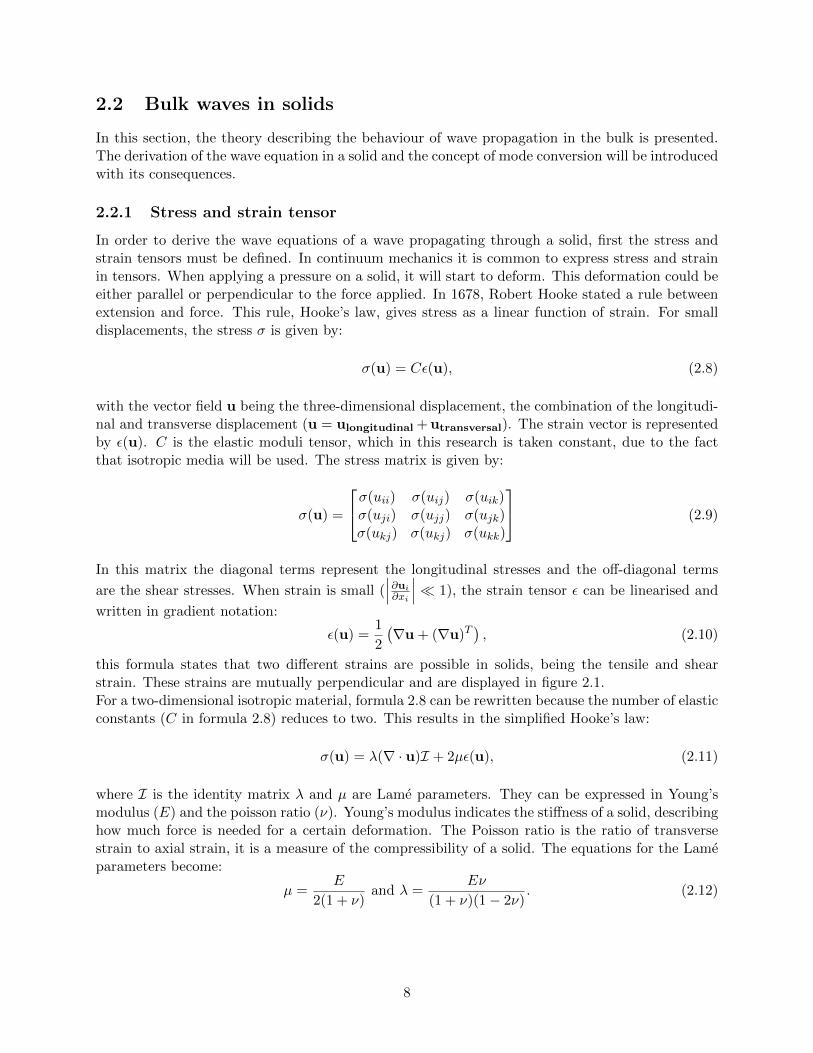
Research done by Foudzi (2014) showed that it is also possible to use polygonal buffer rods as analternative method to reduce the trailing echoes and result in improving the SNR. Instead of using acylindrical buffer rod, the idea is to use a polygonal rod whose normal sectional shape is a polygon.This could be a triangle, square, pentagon etc. [10]. To prove this effectiveness, the idea has beenexamined numerically and experimentally. Triangles, pentagons and heptagons have sides that arenot parallel to any of the other sides. With three-dimensional numerical simulations, they wereproven to cause less interferences among mode converted waves in the rod. This technique enhancesthe SNR partly, but still less spurious echoes are required for a decent viscosity measurementapparatus. Trailing echoes are generated by the interference of the waves due to the bilateralsymmetry shape of the odd polygons. Figure 2.8 shows the cross-sectional shapes of the buffer rodand their 3D simulation model.
The polygons with an odd number of sides (odd-n polygons) were found to give better results thanthe polygons with even number of sides (even-n polygons). Since none of the odd-n polygons haveparallel sides, less trailing echoes were generated and the SNR was improved. The amplitude of thefirst trailing echo for odd-n polygons has been proven to gradually decrease when increasing thenumber of sides. This is due to the fact that the area where such trailing echoes could be formed,decreases. It was found that the biggest area for a possible generation of trailing echoes is that ofa triangle. This idea is shown for odd-n polygons in figure 2.9.
To obtain an ever high SNR, Foudzi’s idea was to use irregular polygons, where at least one ofthe vertices of the polygon is distorted. This influences the symmetry of the polygon, reducing thetrailing echoes. How distorting vertices works is illustrated in figures 2.10 and 2.11.
18
images/area_polygons.png
Figure 2.9: Comparison of the area that contributes to the generation of the first trailing echoesbetween triangle, pentagon and heptagon. [10]
images/regular_hexagon.png
Figure 2.10: Mechanism to generate the first trailing echo for a regular hexagon. It is clearlyvisible that the echoes are focused in the middle of the rod. [10]
images/irregular_hexagon.png
Figure 2.11: Mechanism to generate the first trailing echo for an irregular hexagon. The focusingof the echoes is not as intense as for the regular hexagon. [10]
19
Chapter 3
Simulation model
The simulations done for this research were done in COMSOL Multiphysics. COMSOL Multiphysicsis a cross-platform finite element analysis, solver and multiphysics simulation software. For theultrasonic wave propagation through a solid rod, the Solid Mechanics module will be used. Thischapter will clarify as well as possible the decisions made in simulating the problem.
3.1 General properties in COMSOL
3.1.1 Wave packet
In the beginning process of modelling, definitions and parameters are assigned. The prescribeddisplacement that will be used is a sinusoidal signal multiplied with a Gaussian window, plotted infigure 3.1.
3.1.2 Boundary conditions
There are two important boundary conditions. One describes the behaviour of the boundaryon which the transducer is acting, the other describing all remaining boundaries. A prescribeddisplacement is applied in the direction of the longitudinal axis of the rod, where the transducer isin contact with the boundary. Equation 3.1 gives the displacement on the top surface of the bufferrod.
u = u0,z = −w0 · cos (2πf0) · e− 1
2
(((t−tdelay)·
NP ·tpulse2
)· 6NP ·tpulse
)2
, (3.1)
images/pulse.png
Figure 3.1: Pulse applied on edge of buffer rod, consisting of an infinite sine function multipliedby a Gaussian window.
20
where wo represents the amplitude, f0 the frequency, NP the width of the Gaussian window,tpulse the period of the wave and where tdelay is used to delay the signal and to make sure theentire pulse response will be displayed in the plots. All other boundaries are assumed to be freeboundary conditions, because there, the surrounding air is assumed to be interpreted and simulatedas vacuum. This eliminates all transmissions, so only reflections will be seen in the results.
3.1.3 Dimensions and size
For simulating the buffer rod as a cylinder, a 2-dimensional axial symmetric model is made. Thebuffer rod has a length of 150 mm and a width varying from 20 to 40 mm. Since, as discussedin section 2.7.2, not only cylindrical buffer rods will be studied, it will be necessary to make 3Dmodels. The amount of elements in the mesh will greatly increase because the mesh expands froma flat surface to a 3D volume. For obtaining the same accuracy with a buffer rod of the samesize as for the 2D simulations, the computation time will be much more expensive. To avoid thesimulations running for multiple days, the size of the buffer rod is decreased to 100 mm long and25 mm wide.
3.1.4 Study type
In order to visualise the propagation of the wave, a time-dependent solver will be used. The timeinterval over which it will be calculated is at least 2L
cl, which is the time the ultrasonic wave takes
to propagate up and down the buffer rod. No special solvers are used in the simulations, everythingis calculated by the default solvers of COMSOL Multiphysics.
3.1.5 Materials
Precedent researchers did their simulations for copper only. In the next chapter simulation forboth copper and for titanium are presented. The choice for these materials is that for copper,experiments are already done and for titanium, the software DISPERSE can verify the simulations.This is done by comparing the velocity calculated by DISPERSE with the velocity obtained by post-processing the results of the simulations. The materials that will be used are from the COMSOLmaterials library. The comparison between materials will be done using a Material Sweep, whichis a function in COMSOL Multiphysics.
3.1.6 Measuring in COMSOL
In COMSOL there are multiple ways to measure the behaviour of the ultrasonic wave. To simulatea measurement that behaves like the transducer would in the real experimental setup, the surfaceintegral is calculated at every time point. In structural mechanics, there are multiple ways stresscan be measured. The measured quantity for the wave intensity in the simulations is the secondPiola-Kirchhoff stress (material stress). This stress measurement is defined along the material axisand measures the stress with respect to the original cross-sectional area of the solid [24].
21
3.2 Discretisation of simulation model
The propagation of ultrasonic waves through a buffer rod is done with a finite element method andis a time-dependent problem. It is solved by dividing the time-domain in small time-steps. Not onlythe time-domain, but also the spatial domain is divided into small spatial steps. This discretisationis done by meshing the model. The accuracy of simulations is enhanced by narrowing the mesh-size and by reducing the time-steps. The downside of this is that the computation time increases,because more steps will have to be calculated. Generally, the Nyquist-rate defines that the size ofone mesh element must be at most half the wavelength of the propagating wave. Equivalently, thetime-step size should be smaller than half the period of the highest frequency wave.
3.2.1 Literature review on meshing
An important factor for obtaining an accurate result is the mesh-size of the model. For 2D-axialsymmetric models, there is a simple way for describing the mesh density. A quadrilateral mesh canbe used where the length of one element in the mesh (h) is determined as:
h =λlN, (3.2)
where λl is the longitudinal wavelength and where N represents the number of elements per wave-length. For ultrasonic wave simulations, the number of elements used in literature ranges fromN = 5 up till N = 12.
3.2.2 Meshing in the simulations
The results from the mesh convergence plot in Oud’s study were not completely satisfying. Thefluctuating value of the error, when increasing the mesh density, could not be perfectly explained.Thus, the meshing of the buffer rod simulation will be revised. With the help of an advancedMatlab script, the peaks of the echoes will be detected more carefully and thereby the results areexpected to be more accurate.
3.2.3 Literature review on time-stepping
The time-step is determined by the Courant–Friedrichs–Lewy (CFL) number. In the simulations,the time-step is given by:
∆t =h · CFL
cl, (3.3)
where h is the length of one mesh element (eq. 3.2) and where cl is the longitudinal wave speed. Onestudy concludes that CFL = 0.2 results in accurate simulations with a reasonable computation,another study shows that ∆t = 1/100f gives the optimal result [13], where f is the frequency. Thisis equivalent to CFL = N
100 . In order to make a stable calcukation, the time step can also be chosenaccording to the von Neumann stability criterion:
∆t =h√
cl2 + cs2. (3.4)
This gives for copper, with cl and cs around 4600 and 2300 m/s, a Courant number of 0.8. Oudand Froeling chose for their simulations a Courant number of 0.2. However, this time-step was not
22
used throughout their entire simulation. They only calculated the initial time-step and thereafterthey let COMSOL converge to a time-step.
3.2.4 Time stepping in the simulations
Section 4.2 will present results for different values of the CFL-number and from that, a conclusionwill be drawn. This CFL-number will be used throughout the thesis. In contrast to Oud’s andFroeling’s research, for this thesis a fixed time-stepping will be used. This is because for furtherresearch it is desirable to do spectral analysis of the signal, for which a fixed time-step is required.
23
Chapter 4
Results and discussion
This chapter describes all results obtained from the simulations done in COMSOL Multiphysics5.2a. The results presented here are post-processed using Matlab. Initially, the relation betweenmesh density and accuracy is evaluated, followed by the optimisation of the time-stepping. Theoptimisation of these parameters will be used to eventually do all the other simulations.
4.1 Mesh density
For the 2-dimensional axial symmetric buffer rod, simulations are done to optimise the mesh densitysettings. Simulations are repeated when changing the number of mesh elements per wavelength.The accuracy is tested by calculating the propagation speed of the wave, calculated using a scriptin Matlab (can be found in appendix B). The mesh convergence plot is shown in figure 4.1. Theerror (e) is calculated with:
e = 100 · abs(csim. − ctheor.
ctheor.
), (4.1)
where csim. is the simulated wave speed and where ctheor. is the theoretical wave speed in copper(4600 m/s). The mesh convergence plot shows that from N = 8 and higher the error of the wavespeed becomes lower than 1%. This value will be used for the simulations of the buffer rod.
4.2 Time stepping
For determining the optimal time stepping, the effect of changing time steps is evaluated. For abuffer rod with a length of 150 mm and a diameter of 25 mm, the pulse echoes are measured. Themodel is simulated by varying the time step in the Time-Dependent Solver. The accuracy of thetime-stepping (∆t = h·CFL
cl) increases when the Courant number decreases. For the simulations,
the mesh density was set to N = 8, as was derived as optimal in section 4.1. A superposition ofsome pulse echoes for different Courant numbers is shown in 4.3. The plot shows that a decreaseof the Courant number results in a shift in time of the first reflected peak. As for optimising thenumber of elements per wavelength, for the time discretisation the wave speed is measured as well.The convergence of for the time-stepping is shown in 4.2. It can be concluded that a Courantnumber of 1/10 gives accurate results. For this value, the calculation time was 30 minutes, whichis reasonable. Thus, for the rest of the research in the sections below, this value will be used todefine the time step of the Time-Dependent Solver.
24
images/mesh_convergence_plot.png
Figure 4.1: Mesh convergence plot of an ultrasonic wave propagating through a copper buffer rod,simulated in COMSOL.
images/cfl_convergence.png
Figure 4.2: Time stepping convergence plot of an ultrasonic wave propagating through a copperbuffer rod, simulated in COMSOL
25
images/CFL_normal_zoomed.png
Figure 4.3: Pulse response for different values of the CFL-number, for a rod of 150 mm long and25 mm wide.
Table 4.1: Results of the simulations done for different Courant numbers.
The correctness of the model has been evaluated by comparing it with values found in literatureand experimental data. For a rod of 150 mm with a diameter of 25 mm, the ultrasonic wave of1MHz was prescribed on the top of the rod. For the discretisation of the model, 8 element perwavelength were used with a Courant number of 1/10. The simulation is done for both copper andtitanium.
4.3.1 Copper
The longitudinal wave speed of copper in literature is 4600 m/s. In a experimental study, using acopper buffer rod, Mastromarino verified this sound velocity [1]. The calculation of the longitudinalwave speed (cl) can be done by combining equation 2.19 and 2.12 into:
cl =
√E(1− ν)
ρ(1 + ν)(1− 2ν), (4.2)
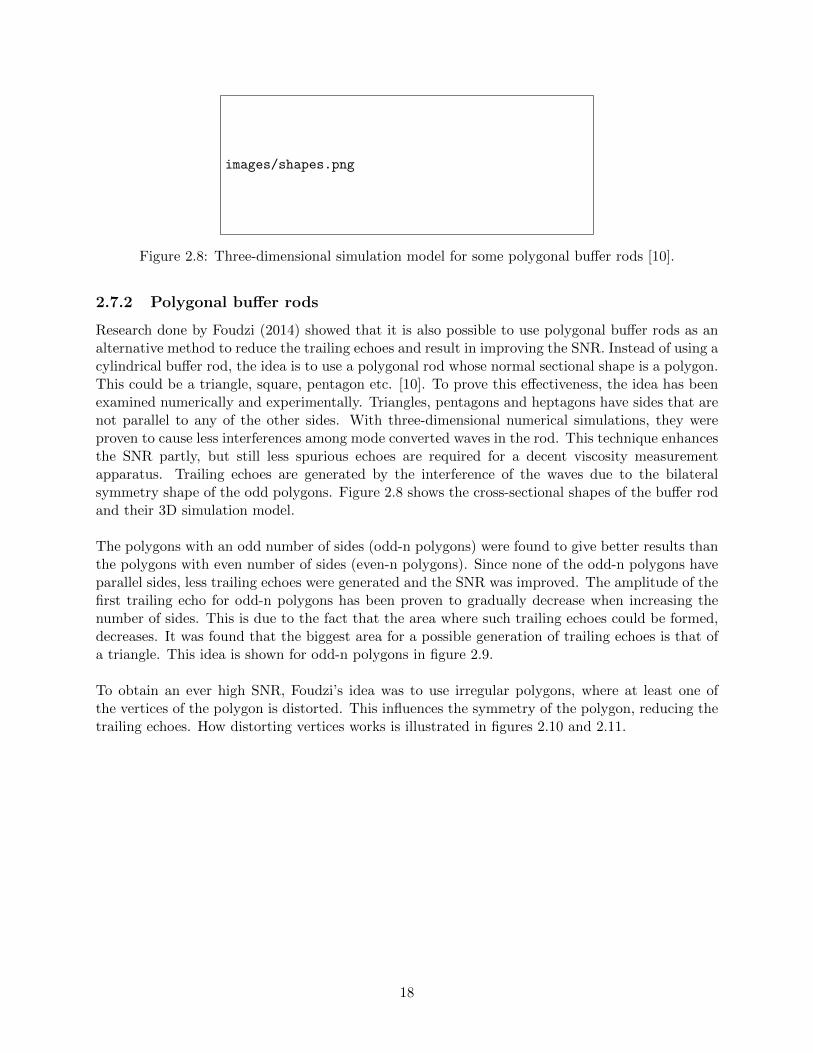
where E is Young’s modulus, ν is Poisson’s ratio and ρ is the density of the solud. With thephysical values of table 4.2, the calculated cl becomes 4607 m/s. To verify the model, the wavespeed is measured by calculating the difference in time between the initial wave and the reflectedwave. This is measured at the top of the buffer rod, where the transducer is placed. Figure 4.4shows the plot of the normalised stress measured at the top of the rod. The horizontal line, close to0, represents the threshold. The script is written in a way that it detects when a smoother versionof the stress measurements exceeds the threshold and it marks the point as the beginning of a peak.
26
Table 4.2: Physical and acoustic properties of the copper and titanium in the built-in library ofCOMSOL [25].
Material Young’s modulus (E) Poisson’s ratio (ν) Density (ρ)
Copper 1.2580 · 1011 0.3350 8.9377 · 103 kg/m3
Titanium 1.0907 · 1011 0.3386 4.4995 · 103 kg/m3
The time travelled is measured as the time between the first and the second peak. This results ina longitudinal wave speed of 4597 m/s.
4.3.2 Titanium
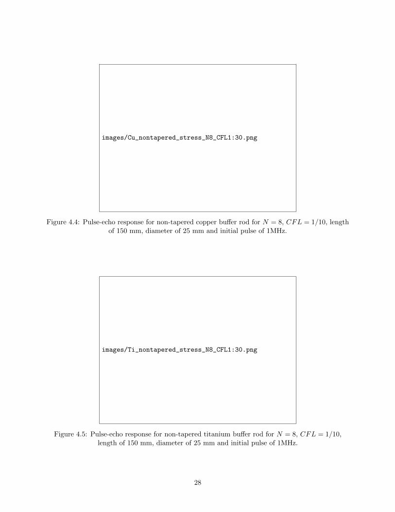
For titanium, the value for the longitudinal wave speed as given by literature is 6070 m/s. Thecalculation of equation 4.2 with the properties of table 4.2 gives the longitudinal wave speed fortitanium as 6091 m/s. Due to the lack of experimental data for a titanium buffer rod, anotherverification method is used. The software package called DISPERSE [20] gives the wave velocity ofsome ultrasonic wave in a solid. This gives 6060 m/s. Because only the demo-licence can be used,this verification method cannot be used for the simulation with copper. Figure 4.5 is a plot of thenormalised stress at the top of the buffer rod. The speed of the wave is calculated as 6050 m/s.Since the values from the simulations in COMSOL are differing by less than 1% of the values of allother sources (see table 4.3), it can be concluded that the model is usable for the simulation of thebuffer rod.
Table 4.3: Values of the longitudinal wave speed, to verify the ultrasonic model in COMSOL.
literature experimental equation 4.2 Disperse COMSOL sim.
Copper 4600 4600 4607.7 - 4597.4
Titanium 6070 - 6091.2 6060 6049.6
27
images/Cu_nontapered_stress_N8_CFL1:30.png
Figure 4.4: Pulse-echo response for non-tapered copper buffer rod for N = 8, CFL = 1/10, lengthof 150 mm, diameter of 25 mm and initial pulse of 1MHz.
images/Ti_nontapered_stress_N8_CFL1:30.png
Figure 4.5: Pulse-echo response for non-tapered titanium buffer rod for N = 8, CFL = 1/10,length of 150 mm, diameter of 25 mm and initial pulse of 1MHz.
28
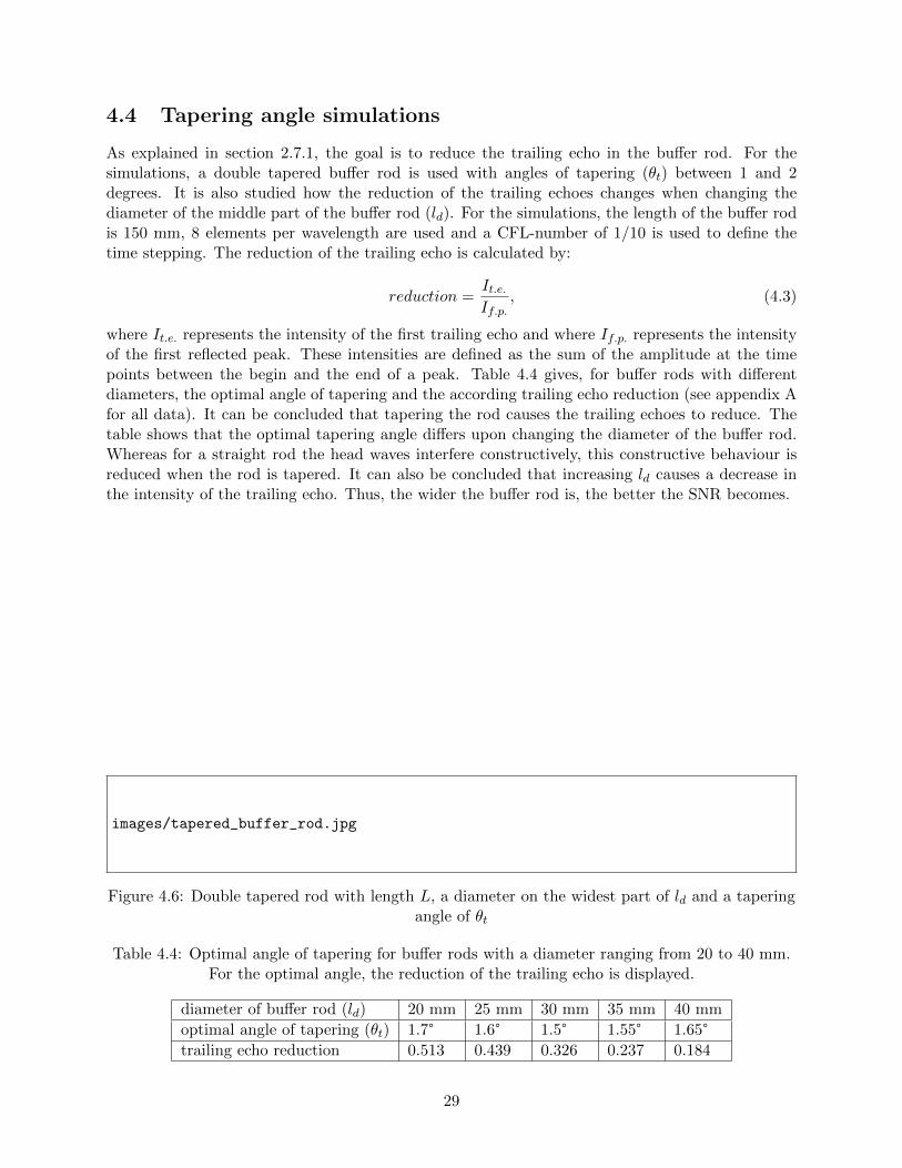
4.4 Tapering angle simulations
As explained in section 2.7.1, the goal is to reduce the trailing echo in the buffer rod. For thesimulations, a double tapered buffer rod is used with angles of tapering (θt) between 1 and 2degrees. It is also studied how the reduction of the trailing echoes changes when changing thediameter of the middle part of the buffer rod (ld). For the simulations, the length of the buffer rodis 150 mm, 8 elements per wavelength are used and a CFL-number of 1/10 is used to define thetime stepping. The reduction of the trailing echo is calculated by:
reduction =It.e.If.p.
, (4.3)
where It.e. represents the intensity of the first trailing echo and where If.p. represents the intensityof the first reflected peak. These intensities are defined as the sum of the amplitude at the timepoints between the begin and the end of a peak. Table 4.4 gives, for buffer rods with differentdiameters, the optimal angle of tapering and the according trailing echo reduction (see appendix Afor all data). It can be concluded that tapering the rod causes the trailing echoes to reduce. Thetable shows that the optimal tapering angle differs upon changing the diameter of the buffer rod.Whereas for a straight rod the head waves interfere constructively, this constructive behaviour isreduced when the rod is tapered. It can also be concluded that increasing ld causes a decrease inthe intensity of the trailing echo. Thus, the wider the buffer rod is, the better the SNR becomes.
images/tapered_buffer_rod.jpg
Figure 4.6: Double tapered rod with length L, a diameter on the widest part of ld and a taperingangle of θt
Table 4.4: Optimal angle of tapering for buffer rods with a diameter ranging from 20 to 40 mm.For the optimal angle, the reduction of the trailing echo is displayed.
diameter of buffer rod (ld) 20 mm 25 mm 30 mm 35 mm 40 mm
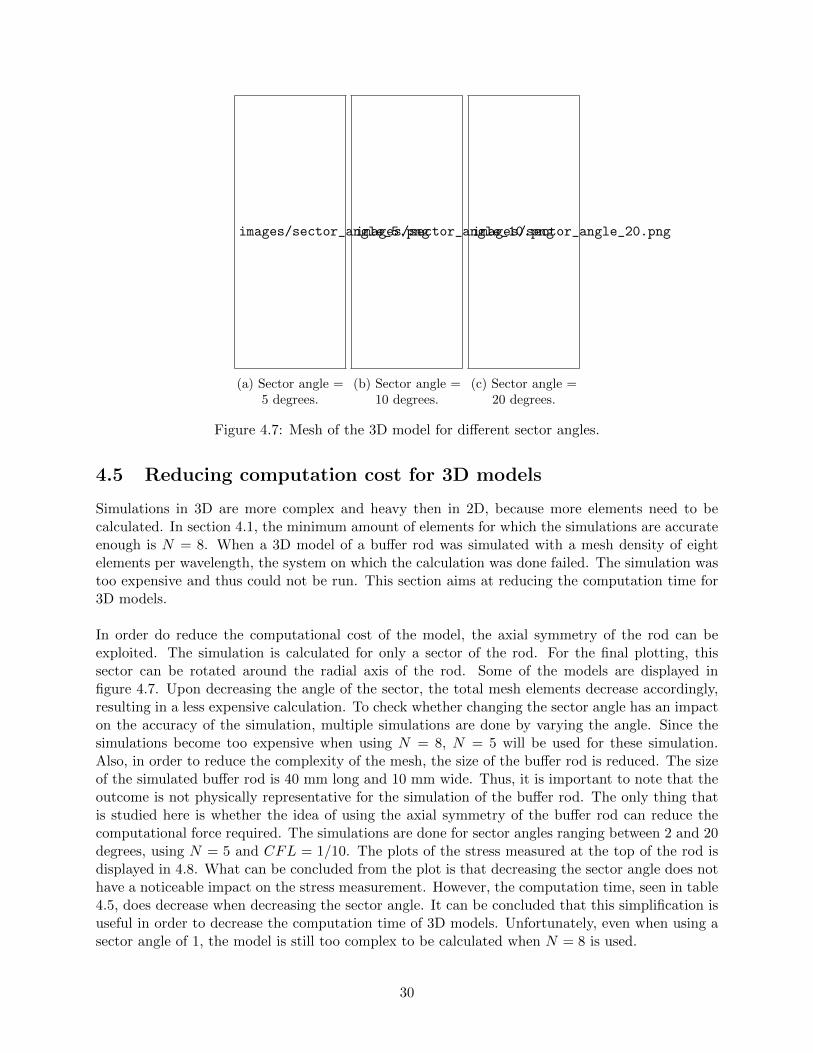
Figure 4.7: Mesh of the 3D model for different sector angles.
4.5 Reducing computation cost for 3D models
Simulations in 3D are more complex and heavy then in 2D, because more elements need to becalculated. In section 4.1, the minimum amount of elements for which the simulations are accurateenough is N = 8. When a 3D model of a buffer rod was simulated with a mesh density of eightelements per wavelength, the system on which the calculation was done failed. The simulation wastoo expensive and thus could not be run. This section aims at reducing the computation time for3D models.
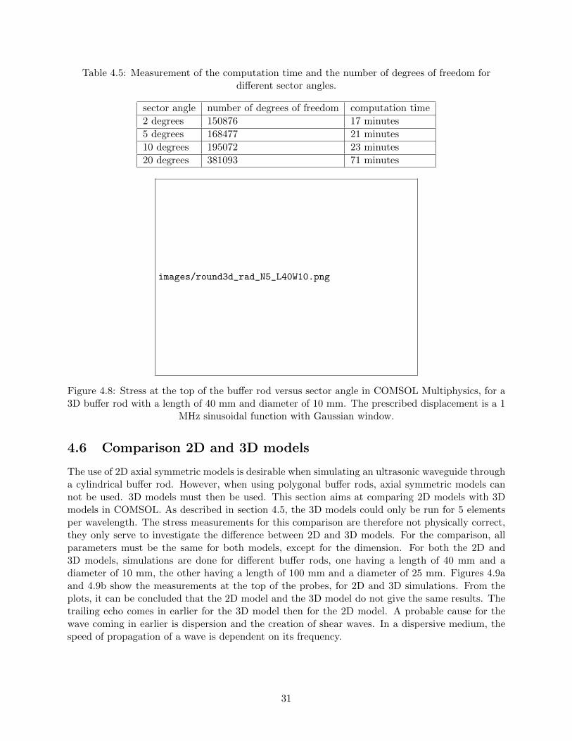
In order do reduce the computational cost of the model, the axial symmetry of the rod can beexploited. The simulation is calculated for only a sector of the rod. For the final plotting, thissector can be rotated around the radial axis of the rod. Some of the models are displayed infigure 4.7. Upon decreasing the angle of the sector, the total mesh elements decrease accordingly,resulting in a less expensive calculation. To check whether changing the sector angle has an impacton the accuracy of the simulation, multiple simulations are done by varying the angle. Since thesimulations become too expensive when using N = 8, N = 5 will be used for these simulation.Also, in order to reduce the complexity of the mesh, the size of the buffer rod is reduced. The sizeof the simulated buffer rod is 40 mm long and 10 mm wide. Thus, it is important to note that theoutcome is not physically representative for the simulation of the buffer rod. The only thing thatis studied here is whether the idea of using the axial symmetry of the buffer rod can reduce thecomputational force required. The simulations are done for sector angles ranging between 2 and 20degrees, using N = 5 and CFL = 1/10. The plots of the stress measured at the top of the rod isdisplayed in 4.8. What can be concluded from the plot is that decreasing the sector angle does nothave a noticeable impact on the stress measurement. However, the computation time, seen in table4.5, does decrease when decreasing the sector angle. It can be concluded that this simplification isuseful in order to decrease the computation time of 3D models. Unfortunately, even when using asector angle of 1, the model is still too complex to be calculated when N = 8 is used.
30
Table 4.5: Measurement of the computation time and the number of degrees of freedom fordifferent sector angles.
sector angle number of degrees of freedom computation time
2 degrees 150876 17 minutes
5 degrees 168477 21 minutes
10 degrees 195072 23 minutes
20 degrees 381093 71 minutes
images/round3d_rad_N5_L40W10.png
Figure 4.8: Stress at the top of the buffer rod versus sector angle in COMSOL Multiphysics, for a3D buffer rod with a length of 40 mm and diameter of 10 mm. The prescribed displacement is a 1
MHz sinusoidal function with Gaussian window.
4.6 Comparison 2D and 3D models
The use of 2D axial symmetric models is desirable when simulating an ultrasonic waveguide througha cylindrical buffer rod. However, when using polygonal buffer rods, axial symmetric models cannot be used. 3D models must then be used. This section aims at comparing 2D models with 3Dmodels in COMSOL. As described in section 4.5, the 3D models could only be run for 5 elementsper wavelength. The stress measurements for this comparison are therefore not physically correct,they only serve to investigate the difference between 2D and 3D models. For the comparison, allparameters must be the same for both models, except for the dimension. For both the 2D and3D models, simulations are done for different buffer rods, one having a length of 40 mm and adiameter of 10 mm, the other having a length of 100 mm and a diameter of 25 mm. Figures 4.9aand 4.9b show the measurements at the top of the probes, for 2D and 3D simulations. From theplots, it can be concluded that the 2D model and the 3D model do not give the same results. Thetrailing echo comes in earlier for the 3D model then for the 2D model. A probable cause for thewave coming in earlier is dispersion and the creation of shear waves. In a dispersive medium, thespeed of propagation of a wave is dependent on its frequency.
31
images/compare2d3d_L40.png
(a) Length = 40 mm, diameter = 10 mm
images/compare2d3d_L100.png
(b) Length = 100 mm, diameter = 40 mm
Figure 4.9: Plot of simulations for two buffer rods, where the stress at the top of the buffer rod ismeasured over time.
4.7 Polygonal buffer rods
Models have been made for the polygonal buffer rods to check the reduction of trailing echoes.The length of these models ranged from 50 mm to 100 mm. Unfortunately, because the bufferrods do not have as many symmetry planes as a circle, the models are too large to be computed.Also, for the simulation of irregular polygonal rods, the symmetry can not be used, since thereis no symmetry. It could be concluded that stronger computer systems are required to study thebehaviour of polygonal buffer rods.
32
Chapter 5
Conclusion
The goal for this research was to optimise a the simulation an ultrasonic wave propagating througha buffer rod. This optimisation was done to save computation time and increase the accuracy.Finally, the optimisation is also necessary to choose the best geometry for the rod and to giveinsight in what experimental set-up will be best to reduce trailing echoes. Reducing trailing echoesresult in and increase of the signal-to-noise ratio. When the SNR increases, the attenuation of awave inside the molten salt can be measured more accurately, thereby making the measurement ofthe viscosity more accurate.
For the discretisation of the model, the optimal amount of elements per wavelength (N) was foundto be 8. The optimisation of the time-discretisation gave a CFL-number of 1/25. These parametersgive an accurate result while also maintaining a reasonable computation time. The simulationscould only be done for 2D axial symmetric models due to a lack of computation power to compute3D models.
This research shows that the optimal angle of tapering differs for different diameters of the bufferrod. When using double tapered buffer rods, the trailing echoes decrease when increasing the rod’sdiameter. However, even after tapering the buffer rod, some trailing echoes are deteriorating themeasurement of the attenuation. This is due to the fact that they are still measured at the sametime as the signals emerging from the liquid. The idea of using polygonal buffer rods seemedpromising, but, due to a lack of computational power it can not be numerically investigated.
5.1 Recommendation
When simulating an ultrasonic wave propagating through a buffer rod in COMSOL, the recom-mendation is to use a mesh with 8 elements per wavelength and to define the time step of theTime-Dependent Solver with a Courant number of 1/10. To increase computation time, the fre-quency can be reduced to 1MHz and the length of the rod for which the simulation is done can alsobe decreased.
Using irregular odd-n polygonal buffer rods can be seen as the potential solution to reduce trailingechoes. Also, the buffer rod could be cladded. This is the addition of a layer around the buffer rodwith a specific acoustic impedance, the converted waves then will be transmitted into the claddinglayer, instead of reflecting at the interface back into the rod.
33
The combination of cladding and using a tapered or polygonal buffer rod will increase the SNR,but still some trailing echoes will deteriorate the signal. Another technique, using surface waves,could potentially give better results. Elastic surface waves, such as Rayleigh or Love waves, cantravel along the surface of a waveguide. When using surface waves, there is no deterioration of themeasurement signal caused by mode conversion. This technique could greatly improve the SNRand could eventually result in accurate measurements of the viscosity and density of fluids at hightemperature.
34
Appendices
35
Appendix A
Measurements for changing taperingangle
Table A.1: Reduction of the trailing echo for a buffer rod with a length of 150 mm and fordifferent diameters.
angle 20 mm 25 mm 30 mm 35 mm 40 mm
1.0 1.471 0.796 0.510 0.399 0.278
1.1 1.297 0.716 0.452 0.364 0.258
1.2 1.109 0.629 0.400 0.324 0.238
1.3 0.965 0.559 0.369 0.288 0.218
1.4 0.816 0.503 0.338 0.260 0.201
1.45 - - 0.328 - -
1.5 0.694 0.470 0.326 0.240 0.190
1.55 - - 0.328 0.237 0.188
1.6 0.585 0.452 0.337 0.238 0.187
1.65 - - - 0.244 0.184
1.7 0.535 0.453 0.371 0.253 0.184
1.75 0.513 - - - -
1.8 0.513 0.449 0.405 0.274 0.187
1.85 0.517 - - - -
1.9 0.535 0.448 0.439 0.301 0.219
2.0 0.553 0.439 0.474 0.328 0.227
2.1 - 0.435 - - -
36
Appendix B
Matlab code for wave speeddetermination
This Matlab script is used to post-process measurements of a parametric sweep in COMSOL. Itcalculated the wave speed by measuring the time of flight of the wave.
Listing B.1: Matlab code for wave speed calculation and measurement plotting
37
Bibliography
[1] Mastromarino, S. (2016). Determination of Thermodynamic properties of Molten Salt, Ph.D.thesis, Delft University of Technology
[2] World Nuclear Association, Generation IV Nuclear Reactors
[4] H. Froeling. Causes of spurious echoes by ultrasonic wave simulation, BSc thesis, Delft Univer-sity of Technology (2017).
[5] J. Serp, M. Allibert, O. Benes, S. Delpech, O, Feynberg, V. Ghetta, D. Heuer, D. Holcomb, V.Ignatiev, J.L. Kloosterman, L. Luzzi, E. Merle-Lucotte, J. Uhlır, R. Yoshioka D. and Zhimin.The molten salt reactor (MSR) in generation IV: Overview and perspectives. Progress in NuclearEnergy, 77:308-319, 2014.
[6] M. Allibert, D. Gerardin, D. Heuer, E. Huffer, A. Laureau, E. Merle, S. Beils, A. Cammi,B. Carluec, S. Delpech, A. Gerber, E. Girardi, J. Krepel, D. Lathouwers, D. Lecarpentier, S.Lorenzi, L. Luzzi, S. Poumerouly, M. Ricotti, and V. Tiberi. Description of initial reference de-sign and identification of safety aspects. Work Package 1, Deliverable D1.1, SAMOFAR (SafetyAssessment of the MOlten Salt FAst Reactor. European project, Contract number: 661891,2016.
[7] T. Oud. Elastic wave simulation for buffer rod tapering. BSc thesis, Delft University of Tech-nology, 2017.
[8] T. Ihara, N. Tsuzuki, and H. Kikura. Development of the ultrasonic buffer rod for the moltenglass measurement, Progress in Nuclear Energy, 82:176–183, 2014.
[9] J. Pezant, J.E. Michaels and T.E. Michaels. An examination of trailing echoes in tapered rods.AIP Conference Proceedings, 1096:1627-1639, 2009.
[10] F.B.M. Foudzi, Development of Polygonal Buffer Rods for Ultrasonic Pulse-Echo Measure-ments with High Signal-to-Noise Ratio. Ph.D. thesis, Nagaoka University of Technology, 2014.
[11] V.S.K. Prasad, K. Balasubramaniama, E. Kannan and K.L.Geisinger, Viscosity measurementsof melts at high temperatures using ultrasonic guided waves, Journal of Materials ProcessingTechnology 207(1):315-320, 2008.
[13] B. Ghose, K. Balasubramaniam, C.V. Krishnamurthy and A.S. Rao, Two dimensional femsimulation of ultrasonic wave propagation in isotropic solid media using comsol, COMSOLConference, 2010.
[14] J.David, N. Cheeke, Fundamentals and applications of ultrasonic waves, CRC Press LLC,2002.
[15] S. Delpech, E. Merle-Lucotte, D. Heuer, M. Allibert, V. Ghetta, C. Le-Brun, X. Doligez andG. Picard. Reactor physic and reprocessing scheme for innovative molten salt reactor system.Journal of Fluorine Chemistry, 2008.
[16] E. Capelli. Thermodynamic characterization of salt components for molten salt reactor fuel.Ph.D thesis, Delft University of Technology, 2016.
[17] R.S. Moore and H.J McSkimin. Dynamic shear properties of solvents and polysterene solutionsfrom 20 to 300 MHz. Physical Acoustics, 6:167-242, 1970.
[18] W.P. Mason, W.O. Baker, H.J McSkimin and J.H. Heiss. Measurement of shear elasticity andviscosity of liquids at ultrasonic frequencies. Physical Review, 75(6): 936-946, 1949.
[19] Reflection and transmission of ultrasonic waves. Retrieved from: http://www.fast.u-psud.
fr/~martin/acoustique/support, n.d.
[20] M. Lowe, Disperse - Guided wave dispersion curve calculation, Imperial College NDT lab, n.d.
[21] Comparison of lifecycle greenhouse gas emission of various electricty generation sources, WNAreport, retreived from: http://www.world-nuclear.org/, 2011.
[22] S. Monkola, Numerical simulation of fluid-structure interaction between acoustic and elasticwaves, Jyvaskyla studies in computing, 133:1456-5390, 2011.
[23] Snells law2.svg. Wikimedia Commons, the free media repository. Retrieved from https://