OPTIMIZATION METHODS FOR LARGE SCALE ... METHODS FOR LARGE SCALE COMBINATORIAL PROBLEMS AND...

OPTIMIZATION METHODS FOR LARGE SCALE

COMBINATORIAL PROBLEMS AND BIJECTIVITY

CONSTRAINED IMAGE DEFORMATIONS

ANDERS ERIKSSON

Faculty of EngineeringCentre for Mathematical Sciences

Mathematics

MathematicsCentre for Mathematical SciencesLund UniversityBox 118SE-221 00 LundSweden

http://www.maths.lth.se/

Doctoral Theses in Mathematical Sciences 2008:2ISSN 1404-0034

ISBN 978-91-628-7417-9LUTFMA-1029-2008 © Anders Eriksson, 2008

Printed in Sweden by MEDIA-TRYCK, Lund 2008

Preface

The thesis is based on the following work

1. Eriksson, A., Olsson, C. and Kahl F., Efficiently Solving the Fractional Trust Re-gion Problem. In Asian Conference on Computer Vision, ACCV, Tokyo, Nov. 2007.

2. Eriksson, A., Olsson, C. and Kahl F., Normalized Cuts Revisited: A Reformulationfor Segmentation with Linear Grouping Constraints. In International Conferenceon Computer Vision, ICCV, Brazil, Oct. 2007.

3. Olsson, C., Eriksson, A. and Kahl F., Improved Spectral Relaxation Methods forBinary Quadratic Optimization Problems Submitted to Journal of Computer Visionand Image Understanding, 2007.

4. Olsson, C., Eriksson, A. and Kahl F., Solving Large Scale Binary Quadratic Prob-lems: Spectral Methods vs. Semidefinite Programming. Proc. CVPR, Minneapolis,USA, 2007.

5. Eriksson, A., Olsson, C. and Kahl F., Segmenting with Context. Proc. SCIA, Aal-borg, Denmark, 2007.

6. Eriksson, A. and Åström, K., Image Registration using Thin-Plate Splines. In Proc.ICPR, Hong Kong, China, 2006.

7. Eriksson, A., Barr, O. and Åström, K. Image Segmentation Using Minimal GraphCuts. To appear Proc. SSBA Symposium on Image Analysis, Umeå, Sweden, 2006.

8. Eriksson, A. and Åström, K., On the Bijectivity of Thin-plate Splines. In Proc.SSBA Symposium on Image Analysis, Malmö, Sweden, 2005.

9. Eriksson, A., Licentiate thesis, Lund University, 2005.

Subsidiary Papers

10. Eriksson, A. and Åström, K., Robustness and specificity in object detection. InProc. ICPR, Cambridge, UK, 2004.

11. Balkenius, C., Åström, K. and Eriksson, A. Learning in visual attention, In Proc. ofInternational Workshop on Learning for Adaptable Visual Systems, ICPR, Cambridge,UK, 2004.

1

2

Acknowledgments

I would like to express my gratitude to all those who gave me the possibility to completethis thesis.

I want to thank my department for giving me opportunity to commence my studiesin the first place.

I am deeply indebted to my supervisor Kalle Åström. Without his unyielding supportand seemingly infinite patience this work would have never been completed. During mytime here he has always provided encouragement, sound advice, lots of good ideas andvery good company.

All the members of the Mathematical Imaging Group has supported me tremendouslyin my work. I would especially like to thank Carl Olsson and Fredrik Kahl who providedinvaluable assistance and advice as well as many interesting discussions. It has been apleasure working with you both.

Finally, I would also like to thank all my colleagues at the department for their help,support, interest and valuable hints and for making my time here so much more enjoy-able.

3

4

Introduction

1 Background

The field of computer vision has, ever since it emerged in the 60’s, been full of opti-mization problems. Looking back, the subfield where optimization perhaps first made animpact was in projective geometry. Structure and motion problems were early on solvedeither by local methods or some algebraic approach, or a combination of both. Typicalexamples of this are the 8-point algorithm [11] and bundle adjustment [9]. For a longtime this was the predominant approach, either the problem was reformulated in such away that it could be easily solved or one employed some local refinement method directlyto the problem at hand. This usually either resulted in a formulation that lacked a mean-ingful connection to the original problem or in the latter case in a solution which onecould not be certain was the desired one. It is only in the last decade that optimizationtheory has received the attention it perhaps rightly deserves within this field. Recently sev-eral publications have appeared that address the issue of how to appropriately formulatea wide variety of optimization problems in computer vision. Formulations with objectivefunctions that has a definite relevance to the problem at hand. And stated in such a waythat they, not only can be efficiently solved, but where one can also say something aboutthe quality of the solution obtained. Examples of such work includes the L∞-norm for-mulations of [8] and [10], the Gröbner base approach of [15] and the branch-and-boundtechnique of [1] Here terms such as convexity and globally optimal solutions are central.

Discrete optimization techniques are possibly not as commonly occurring in com-puter vision as their continuous counterpart, but whose relevance has still proven to beconsiderable. Vision problems as varying as image segmentation and grouping, imageenhancement and denoising, motion segmentation, tracking and object recognition canbe formulated as discrete, or combinatorial, optimization problems. The work that per-haps popularized discrete techniques and first reached a wider audience within the fieldwas the normalized cuts approach of [14]. This method, based on spectral relaxationtechniques, has successfully been used in a wide variety of applications. However, thediscrete optimization technique that lately has received the most attention is the graphcut algorithm of [4]. This is a method that can exactly minimize certain objective func-tionals in polynomial time. Its attraction can be attributed to a thorough understandingof both its underlying theory as well as the properties of the set of problems to which itcan be applied. Several implementations of this method with exceptional computationalcomplexity are also widely available.

Even though continuous and discrete optimization techniques for vision problems

1

Introduction

has largely evolved separately they are closely related. It can also be argued on a purelytheoretical basis that they share a common underlying framework. In addition, with theabove exception, most combinatorial problems that arise in computer vision are knownto be NP-hard and can not be solved optimally in reasonable time. A common approachis to instead look for an approximate solution to the combinatorial problem by droppingthe discrete constraints, a process called relaxation, thus turning the problem into a con-tinuous one that can be solved efficiently. The first half of this thesis deals with discreteoptimization problems of this category.

Next we will present a brief overview of the two applications treated in this thesis.Followed by a an introduction to some of the basic concepts in optimization theory. Inthe final section of this introduction a more detailed summary of the separate papers isgiven.

2 Overview

This thesis treats two separate but connected themes. Namely, image segmentation andimage deformation. This affiliation originates in optimization being the common choiceof method for solving most of the occurring challenges.The thesis consists of the following six segments of work:

I Eriksson, A., Olsson, C. and Kahl F., Normalized Cuts Revisited: A Reformulation forSegmentation with Linear Grouping Constraints, In Proc. International Conferenceon Computer Vision, ICCV, Brazil, Oct. 2007.

II Eriksson, A., Olsson, C. and Kahl F., Efficiently Solving the Fractional Trust RegionProblem, In Proc. Asian Conference on Computer Vision, ACCV, Tokyo, Nov.2007.

III Olsson, C., Eriksson, A. and Kahl F., Improved Spectral Relaxation Methods forBinary Quadratic Optimization Problems, Submitted to Journal of Computer Visionand Image Understanding, 2007.

IV Eriksson, A., Bijective Thin-Plate Splines, In Licentiate thesis, chapter 2, Lund Uni-versity, 2005.

V Eriksson, A. and Kalle Åström, Image Registration using Thin-Plate Splines, In Proc.International Conference on Pattern Recognition, ICPR, Hong Kong, China, 2006.

VI Eriksson, A., Groupwise Image Registration and Automatic Active Appearance ModelGeneration, In Licentiate thesis, chapter 4, Lund University, 2005.

The first theme of the thesis is image segmentation. This is usually defined as thetask of distinguishing objects from background in unseen images. This visual group-ing process is typically based on low-level cues such as intensity, homogeneity or image

2

contours. Popular approaches include thresholding techniques, edge based methods andregion-based methods. Regardless of the method, the difficulty lies in formulating anddescribing the perception of what constitutes foreground and background in an arbitraryimage. Furthermore, such a grouping is also highly contextually driven, certain imageregions may be labeled differently depending on the task at hand - are we looking forpeople, buildings or trees? If one also allows for more labels than only foreground andbackground, the problem becomes increasingly harder and requires a much higher levelof scene understanding.

Once a formulation of the problem has been established and properly stated the ques-tion of how to efficiently solve it still remains. The complexity of this task and the size ofmost natural images typically leads to very large and difficult optimization problems. Itis these issues we make an attempt at addressing in this thesis. We are interested in howto efficiently find visually relevant image partitions as well as how prior information canbe included into the segmentation process.

Figure 1.1: An example of an image segmentation.

The methods investigated in this work is based on techniques from combinatorial op-timization, a choice that was mainly motivated by the proven success of these approaches.Such problems can be stated as large-scale quadratic 0-1 optimization programs with lin-ear constraints. Usually, such proven NP-complete problems are solved by relaxing, orsimply dropping, some constraints and rewriting the problem as one that can be solvedefficiently, In paper I and II we study large scale fractional quadratic 0-1 programs. Wepresent a reformulation of this class of optimization problems that in a unified way canhandle any type of linear equality constraints as well as proposing efficient algorithmsfor solving them. Paper III introduces two new methods for solving binary quadraticproblems that greatly improves on existing and established methods for finding solutionsin the large scale case. Both these proposed methods have been applied to several visionproblems with promising results.

The second theme of this thesis concerns non-linear deformations of images and itsapplications. Functions that map R

2 onto itself are widely used in computer vision,medical imaging and computer graphics. What is common to all three is that mappings

3

Introduction

are used to model deformation occurring in natural images. As such deformations arehighly complex they are near impossible to characterize. A reasonable and widely acceptedassumption, or approximation, is that as the overall structure of the objects depicted willremain intact after deformation, hence folding or tearing of the images should neveroccur, see fig 1.2. Under these premises there must exist a dense mapping that is bothone-to-one and onto. The deformations must be bijective. This is not entirely correct asfor instance self-occlusion can not be described by bijective mappings.

Figure 1.2: Examples of bijective and non-bijective deformations.

There exist an abundance of methods for parameterizing non-linear deformations. Thispart of the thesis concerns conditions for bijectivity of, perhaps the most commonlyused method of describing non-linear deformations, the thin-plate spline mapping and itsapplications in computer vision. Paper IV discusses the thin-plate spline and In paper Vand VI we apply the results of paper IV to the task of pair-wise and group-wise registeringof images.

3 Optimization

This section provides a brief review of some of the basic concepts of optimization, usedin this thesis.

Optimization refers to the task of minimizing (or maximizing) a real-valued functionf : S 7→ R, (the objective function) over a given set S. The term mathematical pro-gramming is also commonly occurring. 1

1The name bears no reference to computer programming but instead originates from the research in op-timization conducted by the United States army in the 1940’s applied to logistical planning and personnelscheduling. “Program” here refers to its military meaning of sequence of operations. The inclusion of this wordsupposedly increased chances for receiving governmental funding at the time.

4

A typical notation is

minx

f(x)

s.t. x ∈ S. (1.1)

The function f is said to have a global minima at x∗ if

f(x) ≥ f(x∗), ∀x ∈ S. (1.2)

The function f is said to have a local minima at x∗ if there is a neighborhood||x − x∗|| < δ such that

f(x) ≥ f(x∗), ∀x ∈ S, ||x − x∗|| < δ. (1.3)

The set S is typically defined by a number of equality constraints, hi(x) = 0, i =1...m and inequality constraints, gi(x) ≤ 0, i = 1...l. The notation becomes

minx

f(x)

s.t. hi(x) = 0, i = 1...m

gi(x) ≤ 0, i = 1...l

x ∈ X, (1.4)

where X is usually some subspace of Rn and hi and gi as well as f are real-valued

functions defined on Rn.

3.1 Unconstrained Optimization

In the absence of any constraints hi and gi, the problem (1.4) is called unconstrained, i.e.simply the task of finding an x∗ that ideally fulfills (1.2), but at least (1.3) over the wholeof X , a subspace of R

n.Despite their apparent limitations, these problems are central to the field of optimiza-

tion. Also many algorithms for solving constrained problems are extensions of methodsfor unconstrained problems. There are numerous algorithms for unconstrained optimiza-tion. In the one-dimensional case there are the sequential methods, such as Dichotomous,Golden-section and Fibonacci search [2]. These very simple yet powerful algorithms pro-duce a sequence of decreasing intervals that converges to a local. They do demand anstarting interval and can only find an optima within this interval. They do not make useof derivatives, a desirable property if f ′ is not readily available.

In multi-dimensional problems, gradient methods, such as steepest descent, use firstorder derivatives to find directions for which the objective function decrease and thenperform one-dimensional line searches in these directions. The Newton method and theconjugate direction exploit the Hessian of the objective function to find search directions.

5

Introduction

In some instances the step length can also be determined directly, eliminating the needfor a line-search.

If f is differentiable, a necessary condition for optimality for unconstrained problemsis the well known condition

∇f = 0. (1.5)

3.2 Constrained Optimization

In this section we describe two important topics in constrained optimization, the conceptof duality and dual problems and the Karush-Kuhn-Tucker conditions.

3.2.1 Karush-Kuhn-Tucker conditions

The Karush-Kuhn-Tucker (KKT) conditions provide necessary conditions for a local op-tima for a constrained optimization problem. They can be interpreted as the constrainedequivalence to (1.5). The Lagrangian function associated with the constrained problem(1.4) is defined as

L(x; λ, ν) = f(x) +

l∑

i=1

λigi(x) +

m∑

j=1

νjhj(x) (1.6)

where x ∈ X and (λ, ν) ∈ D = ν ∈ Rl, λ ∈ R

m, λ ≥ 0. Obviously, for feasible x,λ and ν

L(x; λ, ν) ≤ f(x), (1.7)

since hj(x) = 0, gi(x) ≤ 0 and λi are non-negative. If x∗ is an optimizer of (1.4) it can

be shown that there must exist a λ∗ ≥ 0 such that∑l

i=1λ∗

i gi(x∗) = 0. Thus

f(x∗) = L(x∗; λ∗, ν∗) = f(x) +l∑

i=1

λigi(x) +m∑

j=1

νjhj(x) ≤ f(x∗), (1.8)

6

which implies that the gradient of L(x; λ, ν) with respect to x must be zero. Combiningthis with the feasibility constraints we get the Karush-Kuhn-Tucker conditions,

∇L(x∗; λ∗, ν∗) = ∇f(x) +

l∑

i=1

λi∇gi(x) +

m∑

j=1

νj∇hj(x) = 0 (1.9)

hj(x∗) = 0, j = 1...m (1.10)

gi(x∗) ≤ 0, i = 1...l (1.11)

x∗ ∈ X (1.12)

λi ≥ 0 (1.13)l∑

i=1

λ∗

i gi(x∗) = 0. (1.14)

Here (1.11)-(1.14) are called the feasibility conditions and (1.14) the complementaryslackness condition. One additional requirement for the KKT-conditions to hold is thatthe gradients of the constraints ∇hj and ∇gi are linearly independent at x∗, i.e.

l∑

i=1

λi∇gi(x∗) +

m∑

j=1

νj∇hj(x∗) = 0 ⇒ λ, ν = 0

, (1.15)

also known as the constraint qualification.The conditions that this theorem of Karush-Kuhn-Tucker provide are fundamental

to optimization theory. Many of the existing algorithms for constrained optimization arebased on these KKT-conditions. Such methods can interpreted as trying to identify points(x, λ, ν) that satisfy (1.10)-(1.14), instead of, for instance carrying out line-searches alongdescent directions,

3.2.2 Duality

Given a constrained optimization problem, on the form (1.4), there is another closelyrelated optimization problem called the Lagrangian dual problem. The original problemis accordingly called the primal problem. One of the many remarkable properties of thedual problem is that it is an underestimator of its primal. Thus one can obtain a lowerbound, and in certain instances even the exact minima to the original problem by solvingits dual. This field of Lagrangian duality matured in the 1950’s and led to a flood of newresults that produced countless new optimization algorithms, including some of the mostsuccessful ones in use today.

The Lagrangian dual function of (1.4) is defined as

θ(λ, ν) = infx∈S

L(x; λ, ν). (1.16)

7

Introduction

Clearly,

θ(λ, ν) ≤ L(x; λ, ν) ≤ f(x), (1.17)

for any x ∈ S and λ ≥ 0.The Lagrangian dual is defined as

max θ(λ, ν)

s.t. λ ≥ 0 (1.18)

If λ∗, ν∗ maximize (1.18) the inequality (1.17) still holds and we have that

θ(λ∗, ν∗) ≤ f(x∗). (1.19)

The difference between the maximum of the dual problem and the minima of the primalproblem is called the duality gap, if the duality gap is zero we speak of strong duality.In general, there is a duality gap between the dual and primal problem, but there areinstances when strong duality holds.

Another remarkable property of the Lagrangian dual function is that it is concave,regardless of what the primal problem looks like. Furthermore, the feasible set of the dualproblem is the intersection of a number of halfspaces, λi ≥ 0. Thus solving the dualproblem implies maximizing a concave function over a convex set. This is equivalent to aconvex optimization problem, a topic we will discuss in the next section.

3.2.3 Convex Optimization Problems

Convex optimization problems are a class of problems of special interest to the optimiza-tion community, it is defined as the minimization of a convex function over a convex set.It has long been known that for such problems any local minima is a global minima, theset of global minima is a convex set and that if the objective function is strictly convexthe minima is unique. In optimization convexity it is actually a more important propertythan linearity or non-linearity. Despite this it is only recently that it has become a centraltool in engineering, this can be attributed to recent breakthroughs in convex optimizationalgorithms, most notably the development of the interior point methods [13].

A function f is convex if, for any x and y and 0 ≤ t ≤ 1

f(tx + (1 − t)y) ≥ tf(x) + (1 − t)f(y), (1.20)

see figure 1.3. The function is called concave if −f is convex.

A set C is called convex if the line segment between any two points in C is contained inC. That is, if for any x, y ∈ C and 0 ≤ t ≤ 1

tx + (1 − t)y ∈ C, (1.21)

examples of convex and non-convex sets can be seen in figure 1.4.

8

Figure 1.3: A convex function.

Figure 1.4: A convex set (left) and a non-convex set (right).

Under some mild assumptions, strong duality always hold for convex problems. Thismeans that one can solve convex optimization problem implicitly by maximizing its cor-responding dual problem. It also implies that any point that satisfies the KKT conditionswill give us the minimizer.

Certain commonly occurring convex optimization problems are

• Linear program - minimizing a linear function over the polytope

aTi x ≤ 0, i = 1...n

.

• (Convex) Quadratic program - minimizing a convex quadratic function f overover a polytope

f(x) = xT Hx, H 0.

9

Introduction

• Second-order cone program - minimizing a linear function over the second-ordercone

||Aix − bi||2 ≤ cTi x + di, i = 1...m

.

• Semidefinite program - minimizing a linear function over the intersection of thecone of positive semidefinite matrices and an affine subspace

X 0⋂

Tr(AiX) = bi, i = 1...m .

For a more detailed description of convex optimization we refer to [16].

4 Summary of the papers

PAPER I — Normalized Cuts Revisited: A Reformulation for Segmen-tation with Linear Grouping Constraints.

Indisputably Normalized Cuts is one of the most popular segmentation algorithms incomputer vision. It has been applied to a wide range of segmentation tasks with greatsuccess. A number of extensions to this approach have also been proposed, ones thatcan deal with multiple classes or that can incorporate a priori information in the form ofgrouping constraints. However, what is common for all these suggested methods is thatthey are noticeably limited and can only address segmentation problems on a very specificform. In this paper, we present a reformulation of Normalized Cut segmentation that ina unified way can handle all types of linear equality constraints for an arbitrary numberof classes. This is done by restating the problem and showing how linear constraints canbe enforced exactly through duality. This allows us to add group priors, for example, thatcertain pixels should belong to a given class. In addition, it provides a principled wayto perform multi-class segmentation for tasks like interactive segmentation. The methodhas been tested on real data with convincing results.

Author contribution: This paper was a result of a collaboration between myself,Carl Olsson and Fredrik Kahl. I acted as the primary author with the solid support of mycoauthors. I carried out the experiments and devised the reformulation of the normalizedcut problem. Carl Olsson also contributed with the proof in section 3.

PAPER II — Efficiently Solving the Fractional Trust Region Problem

Normalized Cuts has successfully been applied to a wide range of tasks in computer vi-sion, it is indisputably one of the most popular segmentation algorithms in use today.A number of extensions to this approach have also been proposed, ones that can dealwith multiple classes or that can incorporate a priori information in the form of group-ing constraints. It was recently shown how a general linearly constrained Normalized

10

Cut problem can be solved. This was done by proving that strong duality holds forthe Lagrangian relaxation of such problems. This provides a principled way to performmulti-class partitioning while enforcing any linear constraints exactly.

The Lagrangian relaxation requires the maximization of the algebraically smallesteigenvalue over a one-dimensional matrix sub-space. This is an unconstrained, piece-wisedifferentiable and concave problem. In this paper we show how to solve this optimizationefficiently even for very large-scale problems. The method has been tested on real datawith convincing results.

Author contribution: This paper was a continuation of paper I, with a similar workdistribution. I again acted as the primary author and also carried out the experiments.Carl Olsson contributed with the experimental validation on the artificial problems aswell as choosing the formulation for the second-order derivatives.

PAPER III — Improved Spectral Relaxation Methods for BinaryQuadratic Optimization Problems

In this paper we introduce two new methods for solving binary quadratic problems.While spectral relaxation methods have been the workhorse subroutine for a wide varietyof computer vision problems - segmentation, clustering, subgraph matching to name afew - it has recently been challenged by semidefinite programming (SDP) relaxations. Infact, it can be shown that SDP relaxations produce better lower bounds than spectral re-laxations on binary problems with a quadratic objective function. On the other hand, thecomputational complexity for SDP increases rapidly as the number of decision variablesgrows making them inapplicable to large scale problems.

Our methods combine the merits of both spectral and SDP relaxations - better (lower)bounds than traditional spectral methods and considerably faster execution times thanSDP. The first method is based on spectral subgradients and can be applied to large scaleSDPs with binary decision variables and the second one is based on the trust regionproblem. Both algorithms have been applied to several large scale vision problems withgood performance.

Author contribution: This paper was the result of merging papers [7] and [6]. CarlOlsson acted as primary author of the former and I on the latter, with the constant supportof Fredrik Kahl.

PAPER IV — Bijective Thin-Plate Splines

Thin-plate splines are a class of widely used non-rigid spline mapping functions. It isa natural choice of interpolating function in two dimensions and has been a commonlyused tool for over a decade. Introduced and developed by Duchon [5] and Meinguet[12] and popularized by Bookstein [3], its attractions include an elegant mathematicalformulation along with a very natural and intuitive physical interpretation.

11

Introduction

Consider a thin metal plate extending to infinity in all directions. At a finite numberof discrete positions ti ∈ R

2, i = 1...n, the plate is at fixed heights zi. The metal platewill take then the form that minimizes its bending energy. In two dimensions the bendingenergy of a plate described by a function g(x, y) is proportional to

J(g) =

∫ ∫

R2

(

(

∂2g

∂x2

)2

+ 2

(

∂2g

∂x∂y

)2

+

(

∂2g

∂y2

)2)

dxdy. (1.22)

Consequently, the metal plate will be described by the function that minimizes (1.22)under the point constraints g(ti) = zi. It was proven Duchon [5] that if such a functionexists it is unique.

The thin-plate spline framework can also be employed in a deformation setting, thatis mappings from R

m to Rm. This is accomplished by the combination of several thin-

plate spline interpolants. Here we restrict ourselves to m = 2. If instead of understandingthe displacement of the thin metal plate as occurring orthogonally to the (x1, x2)-planeview them as displacements of the x1- or x2- position of the point constraints. With thisinterpretation, a new function φ : R

2 → R2 can be constructed from two thin-plate

splines, each describing the x1- and x2-displacements respectively.In spite of its appealing algebraic formulation, thin-plate spline mappings do have

drawbacks and, disregarding computational and numerical issues, one in particular. Namely,bijectivity is never assured. In computer vision, non-linear mappings in R

2 of this sortare frequently used to model deformations in images. The basic assumption is that all theimages contain similar structures and therefore there should exist mappings between pairsof images that are both one-to-one and onto. Hence bijective mappings are of interest.

This work is an attempt at characterizing the set of bijective thin-plate spline map-pings. It contains a formulation of how to describe this set, as well as proofs of manyof its properties. It also includes a discussion of some experimentally derived indicationsof other attributes of this set, such as boundedness and convexity, as well as methods forfinding sufficient conditions for bijectivity.

Author contribution: Papers IV-VI were all the result of work carried out by myselfand my advisor Karl Åström. I acted as first author and carried out the experiments in allthree instances.

PAPER V — Image Registration using Thin-Plate Splines

Image registration is the process of geometrically aligning two or more images. In thispaper we describe a method for registering pairs of images based on thin-plate splinemappings. The proposed algorithm minimizes the difference in gray-level intensity overbijective deformations. By using quadratic sufficient constraints for bijectivity and a leastsquares formulation this optimization problem can be addressed using quadratic pro-gramming and a modified Gauss-Newton method. This approach also results in a very

12

computationally efficient algorithm. Example results from the algorithm on three differ-ent types of images are also presented.

PAPER VI — Groupwise Image Registration and Automatic Active Ap-pearance Model Generation

This section is concerned with groupwise image registration, the simultaneous alignmentof a large number of images. As opposed to pairwise registration the choice of referenceimage is not equally obvious, therefore an alternate approach must be taken.

Groupwise registration has received equivalent amounts of attention from the researchcommunity as pairwise registration. It has been especially addressed in shape analysis un-der the name Procrustes analysis.The areas of application are still remote sensing, medicalimaging and computer vision, but now the aggregation of images allows for a greaterunderstanding of their underlying distribution.

The focus here is towards a specific task, the use of image registration to automaticallyconstruct deformable models for image analysis.

13

Introduction

14

Bibliography

[1] S. Agarwal, M.K. Chandraker, F. Kahl, D.J. Kriegman, and S. Belongie. Practi-cal global optimization for multiview geometry. In Proc. 4th European Conf. onComputer Vision, Graz, Austria, pages I: 592–605, 2006.

[2] M. S. Bazaraa, C.M. Shetty, and H. D. Sherali. Nonlinear Programming: Theory andAlgorithms. Wiley-Interscience, second edition, 2006.

[3] F. L. Bookstein. Principal warps: Thin-plate splines and the decomposition ofdeformations. IEEE Trans. Pattern Analysis and Machine Intelligence, 11, 1989.

[4] Y. Boykov, O. Veksler, and R. Zabih. Fast approximate energy minimization viagraph cuts. IEEE Trans. Pattern Analysis and Machine Intelligence, 23(11):1222–1239, 2001.

[5] J. Duchon. Splines minimizing rotation-invariant semi-norms in sobolev spaces.Constructive Theory of Functions of Several Variables, 1987.

[6] A.P. Eriksson, C. Olsson, and F. Kahl. Image segmentation with context. In Proc.Conf. Scandinavian Conference on Image Analysis, Ahlborg, Denmark, 2007.

[7] A.P. Eriksson, C. Olsson, and F. Kahl. Solving large scale binary quadratic problems:Spectral methods vs. semidefinite programming. In Computer Vision and PatternRecognition, 2007.

[8] R. I. Hartley and F. Schaffalitzky. L-∞ minimization in geometric reconstructionproblems. In Proceedings of the IEEE Conference on Computer Vision and PatternRecognition, Washington, DC, June 2004.

[9] R. I. Hartley and A. Zisserman. Multiple View Geometry in Computer Vision. Cam-bridge University Press, ISBN: 0521540518, second edition, 2004.

[10] F. Kahl. Multiple view geometry and the l∞-norm. In ICCV ’05: Proceedingsof the Tenth IEEE International Conference on Computer Vision, pages 1002–1009,Washington, DC, USA, 2005.

[11] H. C. Longuet-Higgins. A computer algorithm for reconstructing a scene from twoprojections. pages 61–62, 1987.

15

Introduction

[12] J. Meinguet. Multivariate interpolation at arbitrary points made simple. Journal ofApplied Mathematics and Physics, 30, 1979.

[13] Y. Nesterov and A. Nemirovskii. Interior-Point Polynomial Algorithms in ConvexProgramming. Society for Industrial and Applied Mathematics, 1994.

[14] J. Shi and J. Malik. Normalized cuts and image segmentation. IEEE Trans. PatternAnalysis and Machine Intelligence, 22(8):888–905, 2000.

[15] H. Stewenius, F. Schaffalitzky, and D. Nister. How hard is 3-view triangulationreally? In ICCV ’05: Proceedings of the Tenth IEEE International Conference on Com-puter Vision (ICCV’05) Volume 1, pages 686–693, Washington, DC, USA, 2005.

[16] L. Vandenberghe and S. Boyd. Convex Optimization. Cambridge University Press,2004.

16

PAPER IIn Pro eedings International Conferen e on Computer Vision,Rio de Janeiro, Brazil 2007.

1

Main Entry: nor · mal · izePronun iation: \'n or-m-,lïz \Fun tion: transitive verbIne ted Form(s): nor · mal · ized; nor · mal · iz · ingOrigin: 1520-1530; from Latin normalis, "in onformity with rule, normal";from from norma, "rule, pattern" literally " arpenter's square" (see norm).1 : to make onform to or redu e to a norm or standard2 : to make normal (as by a transformation of variables)3 : to bring or restore (as relations between ountries) to a normal ondition

Normalized Cuts Revisited: AReformulation for Segmentation with

Linear Grouping Constraints

Anders P. Eriksson, Carl Olsson and Fredrik Kahl

Centre for Mathematical SciencesLund University, Sweden

Abstract

Indisputably Normalized Cuts is one of the most popular segmentation algo-rithms in computer vision. It has been applied to a wide range of segmentationtasks with great success. A number of extensions to this approach have also beenproposed, ones that can deal with multiple classes or that can incorporate a pri-ori information in the form of grouping constraints. However, what is commonfor all these suggested methods is that they are noticeably limited and can onlyaddress segmentation problems on a very specific form. In this paper, we presenta reformulation of Normalized Cut segmentation that in a unified way can han-dle all types of linear equality constraints for an arbitrary number of classes.This is done by restating the problem and showing how linear constraints canbe enforced exactly through duality. This allows us to add group priors, for ex-ample, that certain pixels should belong to a given class. In addition, it providesa principled way to perform multi-class segmentation for tasks like interactivesegmentation. The method has been tested on real data with convincing results.

1 Image Segmentation

Image segmentation can be defined as the task of partitioning an image into disjointsets. This visual grouping process is typically based on low-level cues such as intensity,homogeneity or image contours. Existing approaches include thresholding techniques,edge based methods and region-based methods. Extensions to this process includes the

1

PAPER I

incorporation of grouping constraints into the segmentation process. For instance theclass labels for certain pixels might be supplied beforehand, through user interaction orsome completely automated process, [8, 2].

Currently the most successful and popular approaches for segmenting images arebased on graph cuts. Here the images are converted into undirected graphs with edgeweights between the pixels corresponding to some measure of similarity. The ambitionis that partitioning such a graph will preserve some of the spatial structure of the im-age itself. These graph methods based were made popular first through the NormalizedCut formulation of [9] and more recently by the energy minimization method of [3].This algorithm for optimizing objective functions that are submodular has the propertyof solving many discrete problems exactly. However, not all segmentation problems canbe formulated with submodular objective functions, nor is it possible to incorporate alltypes of linear constraints.

The work described here concerns the former approach, Normalized Cuts, the rele-vance of linear grouping constraints and how they can be included in this framework. It isnot the aim of this paper to argue the merits of one method, or cut metric, over another,nor do we here concern ourselves with how the actual grouping constraints are obtained.Instead we will show how through Lagrangian relaxation one in a unified can handle suchlinear constrains and also in what way they influence the resulting segmentation.

1.1 Problem Formulation

Consider an undirected graph G, with nodes V and edges E and where the non-negativeweights of each such edge is represented by an affinity matrix W , with only non-negativeentries and of full rank. A min-cut is the non-trivial subset A of V such that the sum ofedges between nodes in A and its complement is minimized, that is the minimizer of

cut(A, V ) =∑

i∈Aj∈V \A

wij (1.1)

This is perhaps the most commonly used method for splitting graphs and is a well knownproblem for which very efficient solvers exist. It has however been observed that thiscriterion has a tendency to produced unbalanced cuts, smaller partitions are preferred tolarger ones.

In an attempt to remedy this shortcoming, Normalized Cuts was introduced by [9].It is basically an altered criterion for partitioning graphs, applied to the problem of per-ceptual grouping in computer vision. By introducing a normalizing term into the cutmetric the bias towards undersized cuts is avoided. The Normalized Cut of a graph isdefined as

Ncut =cut(A, V )

assoc(A, V )+

cut(B, V )

assoc(B, V ), (1.2)

2

2. NORMALIZED CUTS WITH GROUPING CONSTRAINTS

where A ∪ B = V , A ∩ B = ∅ and the normalizing term defined as assoc(A, V ) =∑

i∈A,j∈V wij . It is then shown in [9] that by relaxing (1.2) a continuous underestimatorof the Normalized Cut can be efficiently computed. These techniques are then extendedin [11] beyond graph bipartitioning to include multiple segments, and even further in[12] to handle certain types of linear equality constraints.

One can argue that the drawbacks of this, the classical formulation, for solving theNormalized Cut are that firstly obtaining a discrete solution from the relaxed one canbe problematic. Especially in multiclass segmentation where the relaxed solution is notunique but consists of an entire subspace. Furthermore, the set of grouping constraintsis also very limited, only homogeneous linear equality constraints can be included in theexisting theory. We will show that this excludes many visually relevant constraints. In[4] an attempt is made at solving a similar problem with general linear constraints. Thisapproach does however effectively involve dropping any discrete constraint all together,leaving one to question the quality of the obtained solution.

2 Normalized Cuts with Grouping Constraints

In this section we propose a reformulation of the relaxation of Normalized Cuts thatin a unified way can handle all types of linear equality constraints for any number ofpartitions. First we show how we through duality theory reach the suggested relaxation.The following two sections then show why this formulation is well suited for dealing withgeneral linear constraints and how this proposed approach can be applied to multiclasssegmentation.

Starting off with (1.2), the definition of Normalized Cuts, the cost of partitioning animage with affinity matrix W into two disjoint sets, A and B, can be written as

Ncut =

∑

i∈Aj∈B

wij

∑i∈Aj∈V wij

+

∑

i∈Bj∈A

wij

∑

i∈Bj∈V

wij

. (1.3)

Let z ∈ −1, 1n be the class label vector, W the n × n-matrix with entries wij , d

the n × 1-vector containing the row sums of W , and D the diagonal n × n-matrix withd on the diagonal. A 1 is used to denote vectors of all ones. We can write (1.3) as

Ncut =P

i,jwij(zi−zj)

2

2P

i(zi+1)di

+P

i,jwij(zi−zj)

2

2P

i(zi−1)di

=

= zT (D−W )z2dT (z+1) + zT (D−W )z

2dT (z−1) =

=(zT (D−W )z)dT 1

1T ddT 1−zT dT dT z=

(zT (D−W )z)dT 1

zT ((1T d)D−ddT )z . (1.4)

In the last inequality we used the fact that 1T d = zT Dz. When we include general linearconstraints on z on the form Cz = b, C ∈ R

m×n, the optimization problem associated

3

PAPER I

with this partitioning cost becomes

infz

zT (D−W )zzT ((1T d)D−ddT )z

s.t. z ∈ −1, 1n

Cz = b. (1.5)

The above problem is a non-convex, NP-hard optimization problem. Therefore we areled to replace the z ∈ −1, 1n constraint with the norm constraint zT z = n. Thisgives us the relaxed problem

infz

zT (D−W )zzT ((1T d)D−ddT )z

s.t. zT z = n

Cz = b. (1.6)

This is also a non-convex problem, however we shall see in section 3 that we are able tosolve this problem exactly. Next we will write problem (1.6) in homogenized form, thereason for doing this will become clear later on. Let L and M be the (n + 1) × (n + 1)matrices

L =[

(D−W ) 00 0

], M =

[((1T d)D−ddT ) 0

0 0

]

, (1.7)

and

C = [C − b] (1.8)

the homogenized constraint matrix. The relaxed problem (1.6) can now be written

infz

[ zT 1 ]L[ z1 ]

[ zT 1 ]M[ z1 ]

s.t. zT z = n

C [ z1 ] = 0. (1.9)

Finally we add the artificial variable zn+1. Let z be the extended vector[zT zn+1

]T.

Throughout the paper we will write z when we consider the extended variables and justz when we consider the original variables. The relaxed problem (1.6) in its homogenizedform is

infz

zT LzzT Mz

s.t. z2n+1 − 1 = 0

zT z = n + 1

Cz = 0. (1.10)

4

3. LAGRANGIAN RELAXATION AND STRONG DUALITY

Note that the first constraint is equivalent to zn+1 = 1. If zn+1 = −1 then we maychange the sign of z to obtain a solution to our original problem.

The homogenized constraints Cz = 0 now form a linear subspace and can be elim-inated in the following way. Let N

Cbe a matrix where its columns form a base of the

nullspace of C . Let k + 1 be the dimension of the nullspace. Any z fulfilling Cz = 0can be written z = N

Cy, where y ∈ R

k+1. As in the case with the z-variables, y is thevector containing all variables whereas y is a vector containing all but the last variable.Assuming that the linear constraints are feasible we may always choose that basis such

that yk+1 = zn+1 = 1. We put L = NT

CLN

C, M = NT

CMN

C. In the new space we

get the following formulation

infy

f(y) = yT Ly

yT My

s.t. y2k+1 − 1 = 0

yT NT

CN

Cy = ||y||2N

C= n + 1. (1.11)

A common approach to solving this kind of problem is to simply drop one of the twoconstraints. This may however result in very poor solutions. We shall see that we can infact solve this problem exactly without excluding any constraints.

3 Lagrangian Relaxation and Strong Duality

In this section we will show how to solve (1.6) using Lagrange duality. To do this we startby generalizing a lemma from [7] for trust region problems

Lemma 1. If there exists a y with yT A3y + 2bT3 y + c3 < 0, then, assuming the existence

of a minima, the primal problem

infy

yT A1y + 2bT1 y + c1


, s.t yT A3y + 2bT3 y + c3 ≤ 0 (1.12)

and the dual problem

supλ≥0

infy

yT (A1 + λA3)y + (b1 + λb3)T y + c1 + λc3


(1.13)

has no duality gap.

Proof. The primal problem can be written as

inf γ1

s.t yT (A1 − γ1A2)y + 2(b1 − γ1b2)T y + c1 − γ1c2 ≤ 0

yT A3y + 2bT3 y + c3 ≤ 0

(1.14)

5

PAPER I

Let M(λ, γ) be the matrix

M(λ, γ) =[

A1+λA3−γA2 b1+λb3−γb2

(b1+λb3−γb2)T c1+λc3−γc2

]

. (1.15)

The dual problem can be written

supλ≥0 infγ2,y γ2

s.t

[y

1

]T

M(λ, γ2)

[y

1

]

≤ 0.(1.16)

Since (1.16) is dual to (1.14) we have that for their optimal values, γ∗2 ≤ γ∗

1 must hold.To prove that there is no duality gap we must show that γ∗

2 = γ∗1 . We do this by

considering the following problem

supγ3,λ≥0 γ3

s.t M(λ, γ3) 0.(1.17)

Here M(λ, γ3) 0 means that M(λ, γ3) is positive semidefinite. We note that ifM(λ, γ3) 0 then there is no y fulfilling

[y

1

]T

M(λ, γ3)

[y

1

]

+ ǫ ≤ 0 (1.18)

for any ǫ > 0. Therefore we must have that the optimal values fulfills γ∗3 ≤ γ∗

2 ≤ γ∗1 . To

complete the proof we show that γ∗3 = γ∗

1 . We note that for any γ ≤ γ∗1 we have that

yT A3y + 2bT3 y + c3 ≤ 0 ⇒

yT (A1 − γA2)y + 2(b1 − γb2)T y + c1 − γc2 ≥ 0.

(1.19)

However according to the S-procedure [1] this is true if and only if there exists λ ≥ 0 suchthat M(λ, γ) 0. Therefore (γ, λ) is feasible for problem (1.17) and thus γ3 = γ1.

We note that for a fixed γ the problem

infy yT (A1 − γA2)y + 2(b1 − γb2)T y + c1 − γc2

s.t. yT A3y + 2bT3 y + c3 ≤ 0

(1.20)

only has an interior solution if A1 − γA2 is positive semidefinite. If A3 is positivesemidefinite then we may subtract k(yT A3y + 2bT

3 y + c3) (k > 0) from the objectivefunction to obtain boundary solutions. This gives us the following corollary.

Corollary 1. Let A3 be positive semidefinite. If there exists a y with yT A3y+2bT3 y+c3 <

0, then the primal problem

infy



, s.t. yT A3y + 2bT3 y + c3 = 0 (1.21)

6

3. LAGRANGIAN RELAXATION AND STRONG DUALITY

and the dual problem

supλ

infy

yT (A1 + λA3)y + (b1 + λb3)T y + c1 + λc3


(1.22)

has no duality gap, (once again assuming that a minima exists for the primal problem).

Next we will show how to solve a problem on a form related to (1.11). Let

A1 =[

A1 b1bT1 c1

]

, A2 =[

A2 b2bT2 c2

]

, A3 =[

A3 b3bT3 c3

]

Theorem 3.1. Assuming the existence of a minima, if A3 is positive definite, then the primalproblem

infyT A3y+2bT

3y+c3=n+1



=

= infyT

A3y=n+1

y2n+1=1

yTA1y

yTA2y(1.23)

and its dual

supt

infyT A3y=n+1

yTA1y + ty2

n+1 − t

yTA2y(1.24)

has no duality gap.

Proof. Let γ∗ be the optimal value of problem (1.11). Then

γ∗ = inf yTA3y=n+1

y2n+1=1

yTA1y

yT A2y

= supt inf yTA3y=n+1

y2n+1=1

yTA1y+ty2

n+1−t

yT A2y

≥ supt inf yT A3y=n+1yT

A1y+ty2n+1−t

yT A2y

≥ supt,λ inf yyT

A1y+ty2n+1−t+λ(yT

A3y−(n+1))

yT A2y

= sups,λ inf y

yTA1y+sy2

n+1−s+λ(yT A3y+yn+12bT3 y+c3−(n+1))

yT A2y=

= supλ infy2n+1

=1yT

A1y+λ(yT A3y+2bT3 y+c3−(n+1))

yT A2y

= supλ infyyT A1y+2bT

1 y+c1+λ(yT A3y+2bT3 y+c3−(n+1))

yT A2y+2bT2

y+c2

= γ∗. (1.25)

7

PAPER I

Where we let s = t+c3λ. In the last two equalities corollary 1 was used twice. The thirdrow of the above proof gives us that

µ∗ = supt

infyT A3y=n+1

yTA1y + ty2

n+1 − t

yTA2y=

= supt

infyT A3y=n+1

yTA1y + ty2

n+1 − t yTA3y

n+1

yTA2y=

= supt

infyT A3y=n+1

yT(

A1 + t(

[ 0 00 1 ] − A3

n+1

))

y

yTA2y(1.26)

Finally, since strong duality holds, we can state the following corollary. [1].

Corollary 2. If t∗ and y∗ solves (1.26), then (y∗)T N y∗ = n + 1 and y∗k+1 = 1. That is,

y∗ is an optimal feasible solution to (1.12).

4 The Dual Problem and Constrained Normalized Cuts

Returning to our relaxed problem (1.11) we start off by introducing the following lemma.

Lemma 2. L and M are both (n + 1) × (n + 1) positive semidefinite matrices of rank

n − 1, both their nullspaces are spanned by n1 = [ 1 ... 1 0 ]T and n2 = [ 0 ... 0 1 ]T .Consequently, L

Cand M

Care also positive semidefinite.

Proof. L is the zero-padded positive semidefinite Laplacian matrix of the affinity matrixW and is hence also positive semidefinite. For M it suffices to show that the matrix(1T d)D − ddT is p.s.d.

vT ((1T d)D − ddT )v =∑

i di

∑

j djv2j − (

∑

i divi)2

=∑

i,j didjvj(vj − vi) =∑

i didivi(vi − vi) +

+∑

i,j<i didjvj(vj − vi) + djdivi(vi − vj) =∑

i,j<i didj(vj − vi)2 ≥ 0, ∀v ∈ R

n (1.27)

The last inequality comes from di > 0 for all i which means that (1T d)D − ddT , andthus also M , are positive semidefinite.

The second statement follows since both Lni = Mni = 0 for i = 1, 2.

8

4. THE DUAL PROBLEM AND CONSTRAINED NORMALIZED CUTS

Next, since

vT Lv ≥ 0, ∀v ∈ Rn ⇒ vT Lv ≥ 0, ∀v ∈ Null(C) ⇒

⇒ wT NC

T LNC

T w ≥ 0, ∀w ∈ Rk ⇒

⇒ wT Lw ≥ 0, w ∈ Rk

it holds that L 0, and similarly for MC

.

Assuming that the original problem is feasible then we have that, as f(y) of problem(1.23) is the quotient of two positive semidefinite quadratic forms and is therefore f(y)non-negative, a minima for the relaxed Normalized Cut problem will exist. Theorem3.1 states that strong duality holds for a program on the form (1.23), if a minima exists.Consequently, we can apply the theory from the previous section directly and solve (1.11)through its dual formulation. Let

EC

= [ 0 00 1 ] −

NT

CN

C

n+1 = NT

C

[− I

n+10

0 1

]

NC

(1.28)

and let θ(y, t) denote the Lagrangian function. The dual problem is then

supt

inf||y||2

NC

=n+1θ(y, t) =

yT (L + tEC

)y

yT My. (1.29)

The inner minimization is the well known generalized Rayleigh quotient, for whichthe minima is given by the algebraically smallest generalized eigenvalue1 of (L

C+ tE

C)

and MC

. Letting λGmin(t) and vG

min(t), denote the smallest generalized eigenvalue and

corresponding generalized eigenvector of (LC

+ tEC

) and M we can write problem(1.29) as

supt

λGmin(L + tE

C, M). (1.30)

It can easily be shown that the minimizer of the inner problem of (1.29) for some t,

is given by a scaling of the generalized eigenvector, y(t) =√

n+1||vG

min(t)||2

NC

)vGmin(t). The

relaxed Normalized Cut problem can thus be solved by finding the maxima of (1.30). Asthe objective function is the point-wise infimum of functions linear in t, it is a concavefunction, as is expected from dual problems. So solving (1.30) means maximizing aconcave function in one variable t, this can be carried out using standard methods forone-dimensional optimization.

Unfortunately, the task of solving large scale generalized eigenvalue problems canbe demanding, especially when the matrices involved are dense, as in this case. This can,

1By generalized eigenvalue of two matrices A and B we mean finding a λ = λG(A, B) and v, ||v|| = 1such that Av = λBv has a solution.

9

PAPER I

however, be remedied, by exploiting the unique matrix structure we can rewrite the gener-alized eigenvalue problem as a standard one. First we note that the generalized eigenvalueproblem Av = λBv is equivalent to the standard eigenvalue problem B−1Av = λv, ifB is non-singular. Furthermore, in large scale applications it is reasonable to assume thatthe number of variables n + 1 is much greater than the number of constraints m. Thenthe base for the null space of the homogenized linear constraints N

Ccan then be written

on the form NC

= [ c c0

I ]. Now we can write

M = [ c c0

I ]T

([

((1T d)D−ddT ) 00 0

]

) [ c c0

I ] =

=

D:=h

D1 00 D2

i

d:=h

d1

d2

i

=[

D2 0

0 cT0 D1c0+1

]

︸︷︷︸

D

+

+[

cT cd1+d2 0

cT0 cT

0 d1 1

]

︸︷︷︸

V

[D1

1−1

]

︸︷︷︸

S

[ c c0

dT1 cT +dT

2 dT1 c0

0 1

]

=

= D + V SV T . (1.31)

Hence, M is the sum of a positive definite, diagonal matrix D and a low-rank correc-tion V SV T . As a direct result of the Woodbury matrix identity [5] we can express the

inverse of M as

M−1 = (D + V SV T )−1 =

= D−1(

I − V (S−1 + V T D−1V )−1V D−1)

. (1.32)

Despite the potentially immense size of the entering matrices, this inverse can be effi-ciently computed since D is diagonal and the size of the square matrices S and (S−1 +V T D−1V ) are both typically manageable and therefore easily inverted. Our general-ized eigenvalue problem then turns into the problem of finding the smallest algebraic

eigenvalue of the matrix M−1L. The dual problem becomes

supt

λmin

((D−1(I − V (S−1 + V T D−1V )−1V D−1)

NC

T (L + tEC

)NC

). (1.33)

Not only does this reformulation provide us with the more familiar, standard eigenvalueproblem but it will also allow for very efficient computations of multiplications of vectors

to this matrix. This is a crucial property, since, even though M−1(L+tEC

) is still dense,

it is the product and sum of diagonal (D−1, EC

), sparse (L, NC

) and low rank matrices(V , S−1). It is a very structured matrix to which iterative eigensolvers can successfully beapplied.

10

4. THE DUAL PROBLEM AND CONSTRAINED NORMALIZED CUTS

In certain cases it might however occur that the quadratic form in the denominator isonly positive semidefinite and thus singular. These instances are easily detected and must

be treated specially. As we then can not invert M and rewrite the problem as a standardeigenvalue problem we must instead work with generalized eigenvalues, as defined in(1.30). This is preferably avoided as this is typically a more computationally demandingformulation, especially since the entering matrices are dense. Iterative methods for finding

generalized methods for structured matrices such as L+tE and M , do however exist [10].Note, that the absence of linear constraints is such a special instance. However, in thatcase homogenization is completely unnecessary, and (1.6) with Cz = b removed, is anstandard unconstrained generalized Rayleigh quotient and the solution is given by thegeneralized eigenvalue λT

G(D − W, (1T d)D − ddT ).Now, if t∗ and y∗ are the optimizers of (1.29), (and consequently also (1.30)), corol-

lary 2 certifies that (y∗)T NT

CN

Cy∗ = n + 1 and that y∗

k+1 = 1. With z∗ =[

z∗

z∗

n+1

]

=

NCy∗ and zn+1 = yk+1, we have that z∗ prior to rounding is the minimizer of (1.6).

Thus we have shown how to, through Lagrangian relaxation, solve the relaxed, linearlyconstrained Normalized Cut problem exactly.

Finally, the solution to the relaxed problem must be discretized in order to obtain asolution to the original binary problem (1.5). This is typically carried out by applyingsome rounding scheme to the solution.

4.1 Multi-Class Constrained Normalized Cuts

Multi-class Normalized Cuts is a generalization of (1.2) for an arbitrary number of parti-tions.

Nkcut =

k∑

l=1

cut(Al, V )

assoc(Al, V ). (1.34)

If one minimizes (1.34) in an iterative fashion, by, given the current k-way partition,finding a new partition while keeping all but two partitions fixed. This procedure isknown as the α − β-swap when used in graph cuts applications, [3]. The associatedsubproblem at each iteration then becomes

Nkcut =

cut(Ai, V )

assoc(Ai, V )+

+cut(Aj , V )

assoc(Aj , V )+

∑

l 6=i,j

cut(Al, V )

assoc(Al, V )=

cut(Ai, V )

assoc(Ai, V )+

cut(Aj , V )

assoc(Aj , V )+ c, (1.35)

where pixels not labeled i or j are fixed. Consequently, minimizing the multi-class sub-problem can be treated similarly to the bipartition problem. At each iteration we have a

11

PAPER I

problem on the form

infz

f(z) = zT (D−W )z−zT ddT z+(1T d)2

s.t. z ∈ −1, 1n

Cz = b, (1.36)

where W, D, C and b will be dependent on the current partition and choice of labels tobe kept fixed. These matrices are obtained by removing rows and columns correspondingto pixels not labeled i or j, the linear constraints must also be similarly altered to onlyinvolve pixels not currently fixed. Given an initial partition, randomly or otherwise,iterating over the possible choices until convergence ensures a multi-class segmentationthat fulfills all constraints. There is however no guarantee that this method will avoidgetting trapped in local minima and producing a sub-optimal solution, but during theexperimental validation this procedure always produced satisfactory results.

5 Experimental Validation

A number of experiments were conducted to evaluate our proposed formulation but alsoto illustrate how relevant visual information can be incorporated into the segmentationprocess through non-homogenous, linear constraints and how this can influence the par-titioning.

All images were gray-scale of approximately 100-by-100 pixels in size. The affin-ity matrix was calculated based on edge information, as described in [6]. The one-dimensional maximization over t was carried out using a golden section search, typicallyrequiring 15 − 20 eigenvalue calculations. The relaxed solution z was discretized bysimply thresholding at 0.

Firstly, we compared our approach with the standard Normalized Cut method, figure1.1. Both approaches produce similar results, suggesting that in the absence of constraints

Figure 1.1: Original image (left), standard Normalized Cut algorithm (middle) and thereformulated Normalized Cut algorithm with no constraints (right).

12

6. CONCLUSIONS

the two formulations are equivalent. However, where our approach has the added advan-tage of being able to handle linear constraints.

The simplest such constraint might be the hardcoding of some pixels, i.e. pixel ishould belong to a certain class. This can be expressed as the linear constraints zi = ±1,i = 1...m. In figure 1.2 it can be seen how a number of such hard constraints influencesthe segmentation of the image in figure 1.1.

Figure 1.2: Original image (left), segmentation with constraints (middle) and constraintsapplied (right).

Another visually significant prior is the size or area of the resulting segments, that isconstraints such as

∑

i zi = 1T z = a. The impact of enforcing limitations on the size ofthe partitions is shown in figure 1.3.

Excluding and including constraints such as, pixel i and j should belong to the sameor separate partitions, zi + zj = 0 or zi − zj = 0, is yet another meaningful constraint.The result of including a combination of all the above types of constraints can be seen infigure 1.4.

Finally, we also performed a multi-class segmentation with linear constraints, figure1.5.

We argue that these results, not only indicate a satisfactory performance of the sug-gested method, but also illustrates the relevance of linear grouping constraints in imagesegmentation and the impact that they can have on the resulting partitioning. Theseexperiments also seem to indicate that even a simple rounding scheme as the one usedhere can often suffice. As we threshold at zero, hard, including and excluding constraintsare all ensured to hold after discretizing. Only the area constraints are not guaranteedto hold, however probably since the relaxed solution has the correct area, thresholding ittypically produces a discrete solution with roughly the correct area.

6 Conclusions

We have presented a reformulation of the classical Normalized Cut problem that allowsfor the inclusion of linear grouping constraints into the segmentation procedure, througha Lagrangian dual formulation. A method for how to efficiently find such a cut, even

13

PAPER I

Figure 1.3: Original image (top left), segmentation without constraints (top middle) andsegmentation boundary and constraints applied (top right). Segmentation with area con-straints, (area=100 pixels) (middle left), segmentation boundary and constraints applied(middle right). Segmentation with area constraints, (area=2000 pixels) (bottom left),segmentation boundary and constraints applied (bottom right).

for very large scale problems, has also been offered. A number of experiments as well astheoretical proof were also supplied in support of these claims.

Improvements to the presented method include, firstly, the one-dimensional searchover t. As the dual function is the point-wise infimum of the eigenvalues of a matrix, it issub-differentiable and utilizing this information should greatly reduce the time requiredfor finding t∗. Another issue that was left open in this work is regarding the roundingscheme. The relaxed solution z is currently discretized by simple thresholding at 0. Eventhough we can guarantee that z prior to rounding fulfills the linear constraints, this is notnecessarily true after thresholding and should be addressed. For simpler constraints, as theones used here, rounding schemes that ensures that the linear constraints hold can easilybe devised. We felt that an in-depth discussion on different procedures for discretizationwas outside the scope of this paper.

Finally, the question of properly initializing the multi-class partitioning should alsobe investigated as it turns out that this choice can affect both the convergence and thefinal result.

14

6. CONCLUSIONS

Figure 1.4: Original image (top left), segmentation without constraints (top middle),segmentation boundary and constraints applied (top right). Segmentation with hard,including and excluding, as well as area constraints, (area=25% of the entire image) (mid-dle left), segmentation boundary and constraints applied (middle right). Segmentationwith constraints, (area=250 pixels) (bottom left), segmentation boundary and constraintsapplied (bottom right). Here a solid line between two pixels indicate an including con-straint, and a dashed line an excluding.

Acknowledgments

This work has been supported by the European Commission’s Sixth Framework Pro-gramme under grant no. 011838 as part of the Integrated Project SMErobotTM , SwedishFoundation for Strategic Research (SSF) through the programme Vision in Cognitive Sys-tems II (VISCOS II), Swedish Research Council through grants no. 2004-4579 ’Image-Based Localisation and Recognition of Scenes’ and no. 2005-3230 ’Geometry of multi-camera systems’.

15

PAPER I

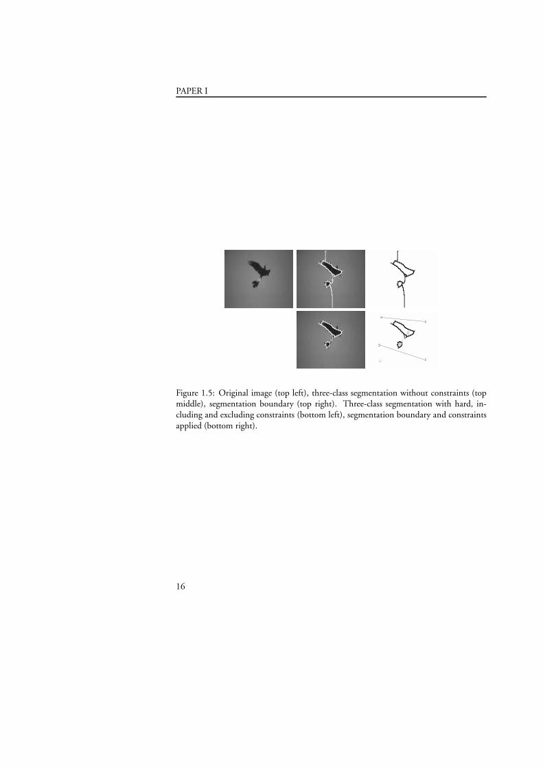
Figure 1.5: Original image (top left), three-class segmentation without constraints (topmiddle), segmentation boundary (top right). Three-class segmentation with hard, in-cluding and excluding constraints (bottom left), segmentation boundary and constraintsapplied (bottom right).

16

Bibliography

[1] S. Boyd and L. Vandenberghe. Convex Optimization. Cambridge University Press, 2004.

[2] Y. Boykov and M.-P. Jolly. Interactive graph cuts for optimal boundary and region segmenta-tion of objects in n-d images. In International Conference on Computer Vision, pages 05–112.Vancouver, Canada, 2001.

[3] Y. Boykov, O. Veksler, and R. Zabih. Fast approximate energy minimization via graph cuts.IEEE Trans. Pattern Analysis and Machine Intelligence, 23(11):1222–1239, 2001.

[4] T. Cour and J. Shi. Solving markov random fields with spectral relaxation. In Proceedings ofthe Eleventh International Conference on Artificial Intelligence and Statistics, volume 11, 2007.

[5] G. H. Golub and C. F. Van Loan. Matrix Computations. Johns Hopkins Studies in Mathe-

matical Sciences, 1996.

[6] J. Malik, S. Belongie, T. K. Leung, and J. Shi. Contour and texture analysis for image seg-

mentation. International Journal of Computer Vision, 43(1):7–27, 2001.

[7] F. Rendl and H. Wolkowicz. A semidefinite framework for trust region subproblems with

applications to large scale minimization. Technical Report CORR 94-32, Departement ofCombinatorics and Optimization, December 1994.

[8] C. Rother, V. Kolmogorov, and A. Blake. ”GrabCut”: interactive foreground extraction using

iterated graph cuts. In ACM Transactions on Graphics, pages 309–314, 2004.

[9] J. Shi and J. Malik. Normalized cuts and image segmentation. IEEE Trans. Pattern Analysisand Machine Intelligence, 22(8):888–905, 2000.

[10] D. C. Sorensen and C. Yang. Truncated QZ methods for large scale generalized eigenvalueproblems. SIAM Journal on Matrix Analysis and Applications, 19(4):1045–1073, 1998.

[11] S. Yu and J. Shi. Multiclass spectral clustering. In International Conference on Computer Vision.Nice, France, 2003.

[12] S. Yu and J. Shi. Segmentation given partial grouping constraints. IEEE Trans. Pattern Analysisand Machine Intelligence, 2(26):173–183, 2004.

17

PAPER IIIn Pro eedings Asian Conferen e on Computer Vision,Tokyo, Japan 2007.

1

Main Entry: ef · · ientPronun iation: \i-'-shnt\Fun tion: adje tiveOrigin: 1350-1400; from Latin e ientem "making"; present parti iple of e- ere "work out, a omplish" (see ee t). Meaning "produ tive, skilled" is from1787.1: being or involving the immediate agent in produ ing an ee t <the e ienta tion of heat in hanging water to steam>2: produ tive of desired ee ts; espe ially : produ tive without waste <ane ient worker>

Efficiently Solving the Fractional TrustRegion Problem

Anders Eriksson, Carl Olsson and Fredrik Kahl


Abstract

Normalized Cuts has successfully been applied to a wide range of tasks in com-puter vision, it is indisputably one of the most popular segmentation algorithmsin use today. A number of extensions to this approach have also been proposed,ones that can deal with multiple classes or that can incorporate a priori informa-tion in the form of grouping constraints. It was recently shown how a generallinearly constrained Normalized Cut problem can be solved. This was done byproving that strong duality holds for the Lagrangian relaxation of such prob-lems. This provides a principled way to perform multi-class partitioning whileenforcing any linear constraints exactly.The Lagrangian relaxation requires the maximization of the algebraically small-est eigenvalue over a one-dimensional matrix sub-space. This is an uncon-strained, piecewise differentiable and concave problem. In this paper we showhow to solve this optimization efficiently even for very large-scale problems. Themethod has been tested on real data with convincing results.

1 Introduction

Image segmentation can be defined as the task of partitioning an image into disjointsets. This visual grouping process is typically based on low-level cues such as intensity,homogeneity or image contours. Existing approaches include thresholding techniques,edge based methods and region-based methods. Extensions to this process includes theincorporation of grouping constraints into the segmentation process. For instance the

1

PAPER II

class labels for certain pixels might be supplied beforehand, through user interaction orsome completely automated process, [9, 3].

Perhaps the most successful and popular approaches for segmenting images are basedon graph cuts. Here the images are converted into undirected graphs with edge weightsbetween the pixels corresponding to some measure of similarity. The ambition is thatpartitioning such a graph will preserve some of the spatial structure of the image itself.These graph based methods were made popular first through the Normalized Cut for-mulation of [10] and more recently by the energy minimization method of [2]. Thisalgorithm for optimizing objective functions that are submodular has the property of thatit solves many discrete problems exactly. However, not all segmentation problems can beformulated with submodular objective functions, nor is it possible to incorporate all typesof linear constraints.

In [5] it was shown how linear grouping constraints can be included in the formerapproach, Normalized Cuts. It was demonstrated how Lagrangian relaxation can in aunified can handle such linear constrains and also in what way they influence the resultingsegmentation. It did not however address the practical issues of finding such solutions.In this paper we develop efficient algorithms for solving the Lagrangian relaxation.

2 Background.

2.1 Normalized Cuts.

Consider an undirected graph G, with nodes V and edges EC

and where the non-negative weights of each such edge is represented by an affinity matrix W , with onlynon-negative entries and of full rank. A min-cut is the non-trivial subset A of V such thatthe sum of edges between nodes in A and V is minimized, that is the minimizer of

cut(A, V ) =∑

i∈A, j∈V \A

wij . (1.1)

This is perhaps the most commonly used method for splitting graphs and is a well knownproblem for which very efficient solvers exist. It has however been observed that thiscriterion has a tendency to produced unbalanced cuts, smaller partitions are preferred tolarger ones.

In an attempt to remedy this shortcoming, Normalized Cuts was introduced by [10].It is basically an altered criterion for partitioning graphs, applied to the problem of per-ceptual grouping in computer vision. By introducing a normalizing term into the cutmetric the bias towards undersized cuts is avoided. The Normalized Cut of a graph isdefined as

Ncut =cut(A, V )

assoc(A, V )+

cut(B, V )

assoc(B, V ), (1.2)

2

2. BACKGROUND.

where A ∪ B = V , A ∩ B = ∅ and the normalizing term defined as assoc(A, V ) =∑

i∈Aj∈V wij . It is then shown in [10] that by relaxing (1.2) a continuous underestima-tor of the Normalized Cut can be efficiently computed.

To be able to include general linear constraints we reformulated the problem in thefollowing way, (see [5] for details). With d = W1 and D = diag(d), Normalized Cutcost can be written as

infz

zT (D − W )z

−zT ddT z + (1T d)2, s.t. z ∈ −1, 1n, Cz = b. (1.3)

The above problem is a non-convex, NP-hard optimization problem. In [5] z ∈ −1, 1n

constraint was replaced with the norm constraint zT z = n. This gives us the relaxedproblem

infz

zT (D − W )z

−zT ddT z + (1T d)2, s.t. zT z = n, Cz = b. (1.4)

Even though this is a non-convex problem it was shown in [5] that it is possible to solvethis problem exactly.

2.2 The Fractional Trust Region Subproblem

Next we briefly review the theory for solving (1.4). If we let z be the extended vector[

zT zn+1

]T. Throughout the paper we will write z when we consider the extended

variables and just z when we consider the original ones. With C = [C − b] the linearconstraints becomes Cz = b, and now form a linear subspace and can be eliminated in the

following way. Let NC

be a matrix where its columns form a base of the nullspace of C .

Any z fulfilling Cz = 0 can be written z = NCy, where y ∈ R

k+1. Assuming that thelinear constraints are feasible we may always choose that basis so that yk+1 = zn+1. Let

LC

= NC

T[

(D−W ) 00 0

]

NC

and MC

= NC

T[

((1T d)D−ddT ) 00 0

]

NC

, both positive

semidefinite, (see [5]). In the new space we get the following formulation

infy

yT LC

y

yT MC

y, s.t. yk+1 = 1, ||y||2N

C

= n + 1, (1.5)

where ||y||2NC

= yT NC

T NC

y. We call this problem the fractional trust region sub-

problem since if the denominator is removed it is similar to the standard trust regionproblem [11]. A common approach to solving problems of this type is to simply dropone of the two constraints. This may however result in very poor solutions. For example,in [4] segmentation with prior data was studied. The objective function considered therecontained a linear part (the data part) and a quadratic smoothing term. It was observedthat when yk+1 6= ±1 the balance between that smoothing term and the data term wasdisrupted, resulting in very poor segmentations.

3

PAPER II

In [5] it was show that in fact this problem can be solved exactly, without excludingany constraints, by considering the dual problem.

Theorem 2.1. If a minima of (1.5) exists its dual problem

supt inf ||y||2N

C

=n+1yT (L

C+tE

C)y

yT MC

y(1.6)

where EC

= [ 0 00 1 ] −

NT

CN

C

n+1 = NT

C

[

− 1n+1

I 0

0 1

]

NC

,

has no duality gap.

Since we assume that the problem is feasible and as the objective function of theprimal problem is the quotient of two positive semidefinite quadratic forms a minimaobviously exists. Thus we can apply this theorem directly and solve (1.5) through itsdual formulation. We will use F (t, y) to denote the objective function of (1.6), theLagrangian of problem (1.5). By the dual function θ(t) we mean the solution of θ(t) =inf ||y||2

NC

=n+1 F (t, y).

The inner minimization of (1.6) is the well known generalized Rayleigh quotient,for which the minima is given by the algebraically smallest generalized eigenvalue 1 of(L

C+ tE

C) and M

C. Letting λmin(·, ·) denote the smallest generalized eigenvalue of

two entering matrices, we can also write problem (1.6) as

supt

λmin(LC

+ tEC

, MC). (1.7)

These two dual formulations will from here on be used interchangeably, it should be clearfrom the context which one is being referred to. In this paper we will develop methodsfor solving the outer maximization efficiently.

3 Efficient Optimization

3.1 Subgradient Optimization

First we present a method, similar to that used in [8] for minimizing binary problemswith quadratic objective functions, based on subgradients for solving the dual formula-tion of our relaxed problem. We start off by noting that as θ(t) is a pointwise infimum offunctions linear in t it is easy to see that this is a concave function. Hence the outer opti-mization of (1.6) is a concave maximization problem, as is expected from dual problems.Thus a solution to the dual problem can be found by maximizing a concave function inone variable t. Note that the choice of norm does not affect the value of θ it only affectsthe minimizer y∗.

1By generalized eigenvalue of two matrices A and B we mean finding a λ = λ(A, B) such that Av =λBv has a solution for some v, ||v|| = 1.

4

3. EFFICIENT OPTIMIZATION

It is well known that the eigenvalues are analytic (and thereby differentiable) functionsas long as they are distinct [6]. Thus, to be able to use a steepest ascent method we needto consider subgradients. Recall the definition of a subgradient [1, 8].

Definition 1. If a function g : Rk+1 7→ R is concave, then v ∈ R

k+1 is a subgradient tog at σ0 if

g(σ) ≤ g(σ0) + vT (σ − σ0), ∀σ ∈ Rk+1. (1.8)

One can show that if a function is differentiable then the derivative is the only vectorsatisfying (1.8). We will denote the set of all subgradients of g at a point t0 by ∂g(t0). Itis easy to see that this set is convex and if 0 ∈ ∂g(t0) then t0 is a global maximum. Nextwe show how to calculate the subgradients of our problem.

Lemma 3.1. If y0 fulfills F (y0, t0) = θ(t0) and ||y0||2NC

= n + 1. Then

v =yT0 E

Cy0

yT0 M

Cy0

(1.9)

is a subgradient of θ at t0. If θ is differentiable at t0, then v is the derivative of θ at t0.

Proof. From (1.6), we get

θ(t) = min||y||2

NC

=1

yT (LC

+ tEC

)y

yT MCy

≤yT0 (L

C+ tE

C)y0

yT0 M

Cy0

=

=yT0 (L

C+ t0EC

)y0

yT0 M

Cy0

+yT0 E

Cy0

yT0 M

Cy0

(t − t0) = θ(t0) + vT (t − t0). (1.10)

3.1.1 A Subgradient Algorithm

Next we present an algorithm based on the theory of subgradients. The idea is to find asimple approximation of the objective function. Since the function θ is concave, the firstorder Taylor expansion θi(t), around a point ti, always fulfills θi(t) ≥ θ(t). If yi solvesinf ||y||2

NC

=n+1 F (y, ti) and this solution is unique then the Taylor expansion of θ at ti

isθi(t) = F (yi, ti) + vT (t − ti). (1.11)

Note that if yi is not unique θi is still an overestimating function since v is a subgradient.One can assume that the function θi approximates θ well in a neighborhood around

t = ti if the smallest eigenvalue is distinct. If it is not we can expect that there is some tjsuch that min(θi(t), θj(t)) is a good approximation. Thus we will construct a functionθ of the type

θ(t) = infi∈I

F (yi, ti) + vT (t − ti) (1.12)

5

PAPER II

that approximates θ well. That is, we approximate θ with the point-wise infimum ofseveral first-order Taylor expansions, computed at a number of different values of t, anillustration can be seen in figure 1.1. We then take the solution to the problem supt θ(t),given by

supt,α α

α ≤ F (yi, ti) + vT (t − ti), ∀i ∈ I, tmin ≤ t ≤ tmax.(1.13)

as an approximate solution to the original dual problem. Here, the fixed parameterstmin, tmax are used to express the interval for which the approximation is believed tobe valid. Let ti+1 denote the optimizer of (1.13). It is reasonable to assume that θ

approximates θ better the more Taylor approximations we use in the linear program.Thus, we can improve θ by computing the first-order Taylor expansion around ti+1, addit to (1.13) and solve the linear program again. This is repeated until |tN+1 − tN | < ǫ

for some predefined ǫ > 0, and tN+1 will be a solution to supt θ(t).

−0.2 −0.1 0 0.1 0.2−3.4

−3.2

−3

−2.8

−2.6

−2.4

−2.2

−2

−1.8

objective functionapproximation

−0.2 −0.1 0 0.1 0.2−5

−4.5

−4

−3.5

−3

−2.5

−2


−0.2 −0.1 0 0.1 0.2−3.4

−3.2

−3

−2.8

−2.6

−2.4

−2.2

−2

−1.8


−0.2 −0.1 0 0.1 0.2−5

−4.5

−4

−3.5

−3

−2.5

−2


Figure 1.1: Approximations of two randomly generated objective functions. Top: Ap-proximation after 1 step of the algorithm. Bottom: Approximation after 2 steps of thealgorithm.

3.2 A Second Order Method

The algorithm presented in the previous section uses first order derivatives only. Wewould however like to employ higher order methods to increase efficiency. This requirescalculating second order derivatives of (1.6). Most formulas for calculating the secondderivatives of eigenvalues involves all of the eigenvectors and eigenvalues. However, de-termining the entire eigensystem is not feasible for large scale systems. We will show that

6

3. EFFICIENT OPTIMIZATION

it is possible to determine the second derivative of an eigenvalue function by solving acertain linear system only involving the corresponding eigenvalue and eigenvector.

The generalized eigenvalues and eigenvectors fulfills the following equations

((LC

+ tEC

) − λ(t)MC

)y(t) = 0 (1.14)

||y(t)||2NC

= n + 1. (1.15)

To emphasize the dependence on t we write λ(t) for the eigenvalue and y(t) for theeigenvector. By differentiating (1.14) we obtain

(EC− λ′(t)M

C)y(t) + ((L

C+ tE

C) − λ(t)M)y′(t) = 0. (1.16)

This (k + 1) × (k + 1) linear system in y′(t) will have a rank of k, assuming λ(k) is adistinct eigenvalue. To determine y′(t) uniquely we differentiate (1.15), obtaining

yT (t)NC

T NC

y′(t) = 0. (1.17)

Thus, the derivative of the eigenvector y′(t) is determined by the solution to the linearsystem

[

(LC

+tEC

)−λ(t)MC

yT (t)NC

T NC

]

y′(t) =[

(−EC

+λ′(t)MC

)y(t)0

]

(1.18)

If we assume differentiability at t, the second derivative of θ(t) can now be found bycomputing d

dtθ′(t), where θ′(t) is equal to the subgradient v given by (1.9).

θ′′(t) = ddt

θ′(t) = ddt

y(t)T EC

y(t)

y(t)T MC

y(t) = 2y(t)T M

Cy(t) y

T (t)(

EC− θ′(t)M

C

)

y′(t)

(1.19)

3.2.1 A Modified Newton Algorithm

Next we modify the algorithm presented in the previous section to incorporate the sec-ond derivatives. Note that the second order Taylor expansion is not necessarily an over-estimator of θ. Therefore we can not use the the second derivatives as we did in theprevious section.

Instead, as we know θ to be infinitely differentiable when the smallest eigenvalue λ(t)is distinct, strictly convex around its optima t∗, Newton’s method for unconstrained op-timization can be applied. It follows from these properties of θ(t) that Newton’s method[1] should be well behaved on this function and that we could expect quadratic conver-gence in a neighborhood of t∗. All of this, under the assumption that θ is differentiablein this neighborhood. Since Newton’s method does not guarantee convergence we havemodified the method slightly, adding some safeguarding measures.

7

PAPER II

At a given iteration of the Newton method we have evaluated θ(t) at a number ofpoints ti. As θ is concave we can easily find upper and lower bounds on t∗ (tmin, tmax)by looking at the derivative of the objective function for these values of t = ti.

tmax = mini;θ′(ti)≤0

ti, (1.20)

tmin = maxi;θ′(ti)≥0

ti. (1.21)

At each step in the Newton method a new iterate is found by approximating the objectivefunction is by its second-order Taylor approximation

θ(t) ≈ θ(ti) + θ′(ti)(t − ti) +θ′′(ti)

2(t − ti)

2. (1.22)

and finding its maxima. By differentiating (1.22) it is easily shown that its optima, as wellas the next point in the Newton sequence, is given by

ti+1 = −θ′(ti)

θ′′(ti)+ ti. (1.23)

If ti+1 is not in the interval [tmin, tmax] then the second order expansion can not bea good approximation of θ, here the safeguarding comes in. In these cases we simply fallback to the first-order method of the previous section. If we successively store the valuesof θ(ti), as well as the computed subgradients at these points, this can be carried out withlittle extra computational effort. Then, the upper and lower bounds tmin and tmax areupdated, i is incremented by 1 and the whole procedure is repeated, until convergence.

If the smallest eigenvalue λ(ti) at an iteration is not distinct, then θ′′(t) is not definedand a new Newton step can not be computed. In these cases we also use the subgradientgradient method to determine the subsequent iterate. However, empirical studies indicatethat non-distinct smallest eigenvalues are extremely unlikely to occur.

4 Experiments

A number of experiments were conducted in an attempt to evaluate the suggested ap-proaches. As we are mainly interested in maximizing a concave, piece-wise differentiablefunction, the underlying problem is actually somewhat irrelevant. However, in orderto emphasize the intended practical application of the proposed methods, we ran thesubgradient- and modified Newton algorithms on both smaller, synthetic problems aswell as on larger, real-world data. For comparison purposes we also include the results ofa golden section method [1], used in [5], as a baseline algorithm.

First, we evaluated the performance of the proposed methods on a large number ofsynthetic problems. These were created by randomly choosing symmetric, positive defi-nite, 100×100 matrices. As the computational burden lies in determining the generalized

8

4. EXPERIMENTS

eigenvalue of the matrices LC

+ tEC

and MC

we wish to reduce the number of suchcalculations. Figure 1.2 shows a histogram of the number of eigenvalue evaluations forthe subgradient-modified Newton method as well as the baseline golden section search.

0 10 20 30 40 500

200

400

600

800

1000

1200

Subgradient alg.Golden section

0 10 20 30 40 500

200

400

600

800

1000

1200

Mod−Newton alg.Golden section

Figure 1.2: Histogram of the number of function evaluations required for 1000-synthetically generated experiments using a golden section method (blue) and the sub-gradient algorithm (red).

The two gradient methods clearly outperforms the golden section search. The differ-ence between the subgradient- and modified Newton is not as discernible. The somewhatsurprisingly good performance of the subgradient method can be explained by the factthat far away from t∗ the function θ(t) is practically linear and an optimization methodusing second derivatives would not have much advantage over one that uses only firstorder information.

Finally, we applied our methods to two real world examples. The underlying mo-tivation for investigating an optimization problem of this form was to segment imageswith linear constraints using Normalized Cuts. The first image can be seen in figure1.3, the linear constraints included were hard constraints, that is the requirement thatthat certain pixels should belong to the foreground or background. One can imagine thatsuch constraints are supplied either by user interaction in a semi-supervised fashion orby some automatic preprocessing of the image. The image was gray-scale, approximately100 × 100 pixels in size, the associated graph was constructed based on edge informa-tion as described in [7]. The second image was of traffic intersection where one wishesto segment out the small car in the top corner. We have a probability map of the im-age, giving the likelihood of a certain pixel belonging to the foreground. Here the graphrepresentation is based on this map instead of the gray-level values in the image. Theapproximate size and location of the vehicle is know and included as linear constraintinto the segmentation process. The resulting partition can be seen in figure 1.4.

In both these real world cases, the resulting segmentation will always be the same,regardless of approach. What is different is the computational complexity of the differentmethods. Once again, the two gradient based approaches are much more efficient thana golden section search, and their respective performance comparable. As the methods

9

PAPER II

0 5 10 15 20 25 30 35 40 45 500

1

2

3

4

5

6

7

8 10 12 14 16 18 20 22 24 26

−0.02

0

0.02

0.04

0.06

0.08

0.1

Figure 1.3: Top: Resulting segmentation (left) and constraints applied (right). Here anX means that this pixel belongs to the foreground and an O to the background. Bot-tom: Convergence of the modified Newton (solid), subgradient (dashed) and the goldensection (dash-dotted) algorithms. The algorithms converged after 9, 14 and 23 iterationrespectively.

differ in what is required to compute, a direct comparison of them is not a straight for-ward procedure. Comparing the run time would be pointless as the degree to which theimplementations of the individual methods have been optimized for speed differ greatly.However, as it is the eigenvalue computations that are the most demanding we believethat comparing the number of such eigenvalue calculations will be a good indicator ofthe computational requirements for the different approaches. It can be seen in figure 1.3and 1.4 how the subgradient methods converges quickly in the initial iterations only toslow down as it approaches the optima. This is in support of the above discussion re-garding the linear appearance of the function θ(t) far away from the optima. We therforeexpect the modified Newton method to be superior when higher accuracy is required.

In conclusion we have proposed two methods for efficiently optimizing a piece-wisedifferentiable function using both first- and second order information applied to the taskof partitioning images. Even though it is difficult to provide a completely accurate com-parison between the suggested approaches it is obvious that the Newton based method issuperior.

10

4. EXPERIMENTS

0 5 10 15 20 25 30

0

0.1

0.2

0.3

0.4

0.5

0.6

0.7

0.8

0.9

1

5 10 15 20 25

−4

−2

0

2

4

6

8

x 10−3

Figure 1.4: Top: Resulting segmentation (left) and constraints applied, in addition tothe area requirement used (area = 50 pixels) (right). Here the X in the top right partof the corner means that this pixel belongs to the foreground. Bottom: Convergence ofthe modified Newton (solid), subgradient (dashed) and the golden section (dash-dotted)algorithms. The algorithms converged after 9, 15 and 23 iteration respectively.

11

PAPER II

12

Bibliography

[1] Bazaraa, Sherali, and Shetty. Nonlinear Programming, Theory and Algorithms. Wiley,2006.

[2] Y. Boykov, O. Veksler, and R. Zabih. Fast approximate energy minimization viagraph cuts. IEEE Trans. Pattern Analysis and Machine Intelligence, 23(11):1222–1239, 2001.

[3] Yuri Boykov and Marie-Pierre Jolly. Interactive graph cuts for optimal boundaryand region segmentation of objects in n-d images. In International Conference onComputer Vision, pages 05–112, Vancouver, Canada, 2001.

[4] A.P. Eriksson, C. Olsson, and F. Kahl. Image segmentation with context. In Proc.Conf. Scandinavian Conference on Image Analysis, Ahlborg, Denmark, 2007.

[5] A.P. Eriksson, C. Olsson, and F. Kahl. Normalized cuts revisited: A reformulationfor segmentation with linear grouping constraints. In International Conference onComputer Vision, Rio de Janeiro, Brazil, 2007.

[6] J. Magnus. On differentiating eigenvalues and eigenvectors. Econometric Theory, 1.

[7] Jitendra Malik, Serge Belongie, Thomas K. Leung, and Jianbo Shi. Contour andtexture analysis for image segmentation. International Journal of Computer Vision,43(1):7–27, 2001.

[8] C. Olsson, A.P. Eriksson, and F. Kahl. Solving large scale binary quadratic problems:Spectral methods vs. semidefinite programming. In Proc. Conf. Computer Vision andPattern Recognition, Mineapolis, USA, 2007.

[9] C. Rother, V. Kolmogorov, and A. Blake. ”GrabCut”: interactive foreground extrac-tion using iterated graph cuts. In ACM Transactions on Graphics, pages 309–314,2004.


[11] D.C. Sorensen. Newton’s method with a model trust region modification. SIAMJournal on Nummerical Analysis, 19(2):409–426, 1982.

13

PAPER IIISubmitted to Computer Vision and Image Understanding, 2007.

1

Main Entry: prob · lemPronun iation:\'prä-blm\Fun tion: nounOrigin: 1350-1400; from Greek problema "a question" literally "thing put for-ward"; from proballein "propose"; from pro "forward" + ballein "to throw"(see ballisti s).1 a: a question raised for inquiry, onsideration, or solutionb: a proposition in mathemati s or physi s stating something to be done2 a: an intri ate unsettled questionb: a sour e of perplexity, distress, or vexation : di ulty in understanding or a epting <I have a problem with your sayingthat>

Improved Spectral Relaxation Methodsfor Binary Quadratic Optimization

Problems

Carl Olsson, Anders P. Eriksson and Fredrik Kahl

Abstract

In this paper we introduce two new methods for solving binary quadratic problems.While spectral relaxation methods have been the workhorse subroutine for a wide varietyof computer vision problems - segmentation, clustering, subgraph matching to name afew - it has recently been challenged by semidefinite programming (SDP) relaxations. Infact, it can be shown that SDP relaxations produce better lower bounds than spectral re-laxations on binary problems with a quadratic objective function. On the other hand, thecomputational complexity for SDP increases rapidly as the number of decision variablesgrows making them inapplicable to large scale problems.

Our methods combine the merits of both spectral and SDP relaxations - better (lower)bounds than traditional spectral methods and considerably faster execution times thanSDP. The first method is based on spectral subgradients and can be applied to large scaleSDPs with binary decision variables and the second one is based on the trust regionproblem. Both algorithms have been applied to several large scale vision problems withgood performance.

1 Introduction

Spectral relaxation methods can be applied to a wide variety of problems in computervision. They have been developed to provide solutions to, e.g., motion segmentation,figure-ground segmentation, clustering, subgraph matching and digital matting [9, 14,21, 26, 12]. In particular, large scale problems that can be formulated with a binaryquadratic objective function are handled efficiently with several thousands of decisionvariables.

More recently, semidefinite programming (SDP) relaxations have also been appliedto the same type of computer vision problems, e.g., [10, 25, 20]. It can be shown that

1

PAPER III

such relaxations produce better estimates than spectral methods. However, as the numberof variables grows, the execution times of the semidefinite programs increase rapidly. Inpractice, one is limited to a few hundred decision variables.

Spectral and SDP relaxation methods can be regarded as two points on an axis ofincreasing relaxation performance. We introduce two alternative methods that lie some-where in between these two relaxations. Unlike standard SDP solvers that suffer frompoor time complexity, they can still handle large scale problems. The two methods arebased on a subgradient optimization scheme. We show good performance on a number ofproblems. Experimental results are given on the following problems: segmentation withprior information, binary restoration, partitioning and subgraph matching. Our maincontributions are:

• An efficient algorithm for solving binary SDP problems with quadratic objectivefunction based on subgradient optimization is developed. In addition, we showhow to incorporate linear constraints in the same program.

• The trust region subproblem is introduced and we modify it to in order to be ap-plicable to binary quadratic problems with a linear term in the objective function.

Many of the application problems mentioned above are known to be NP-hard, soin practice they cannot be solved optimally. Thus one is forced to rely on approximatemethods which results in sub-optimal solutions. Certain energy (or objective) functionalsmay be solved in polynomial time, for example, submodular functionals using graph cuts[11], but this is not the topic of the present paper.

In [8], an alternative (and independent) method is derived which is also based onsubgradients, called the spectral bundle method. Our subgradient method differs from [8]in that it is simpler (just look for an ascent direction) and we have found empiricallyon the experimental problems (see Section 5) that our method performs equally well (orbetter). An in-depth comparison of the two alternatives is, however, beyond the scope ofthis paper.

1.1 Outline

The outline of this paper is as follows: In the next section we present the problem andsome existing approximation techniques for obtaining approximate solutions.

In section 3 we present our algorithm. We develop theory for improving the spectralrelaxation, by using the notion of subgradients. Subgradients is a generalization of gradi-ents that is used when a function is not differentiable. We show that for our problem thesubgradients can be calculated analytically, to determine ascent directions, to be used inan ascending direction scheme.

In section 4 we study the Trust Region Subproblem, which is an interesting specialcase in which we only try to enforce the binary constraints on one of the variables. This

2

2. BACKGROUND

has been extensively studied in the optimization literature and we show that it is alwayspossible to solve exactly.

Finally we test our algorithms and compare with existing methods on the follow-ing problems: segmentation with prior information, binary restoration, partitioning andsubgraph matching. Preliminary results of this work was presented in [15] and [5].

2 Background

In this paper we study different ways to find approximate solutions of the following binaryquadratic problem

z = inf yTAy + bT y, y ∈ −1, 1n, (1)

whereA is an n×n (possibly indefinite) matrix. A common approach for approximatingthis highly nonconvex problem is to solve the relaxed problem:

zsp = inf||x||2=n+1

xTLx, (2)

where

x =

(y

yn+1

)

, L =

(A 1

2b12bT 0

)

.

Solving (2) amounts to finding the eigenvector corresponding to the algebraically smallesteigenvalue of L. Therefore we will refer to this problem as the spectral relaxation of (1).The benefits of using this formulation is that eigenvalue problems of this type are wellstudied and there exist solvers that are able to efficiently exploit sparsity in the matrix L,resulting in fast execution times. A significant weakness of this formulation is that theconstraints y ∈ −1, 1n and yn+1 = 1 are relaxed to ||x||2 = n + 1, which oftenresults in poor approximations.

Now let us turn our attention to bounds obtained through semidefinite program-ming. Using Lagrange multipliers σ = [σ1, . . . , σn+1 ]T for each binary constraintx2i − 1 = 0, one obtains

supσ

infxxT (L+ diag(σ))x − eTσ, (3)

as relaxation of (1). Here e is an (n+ 1)-vector of ones. The inner minimization is finitevalued if and only if (L+diag(σ)) is positive semidefinite, which we write, L+diag(σ) 0. This gives the equivalent relaxation

zd = infσeTσ, L+ diag(σ) 0. (4)

We will denote this problem the dual semidefinite problem since it is dual to the problem

zp = infX0

tr(LX), diag(X) = I, (5)

3

PAPER III

where X denotes a (n + 1) × (n + 1) matrix, as was shown in [3, 10]. Consequentlywe will call this problem the primal semidefinite program. Since the dual problems (4)and (5) are convex, there is in general no duality gap. In [10], the proposed methodis to solve (5) and use randomized hyperplanes (see [7]) to determine an approximatesolution to (1). This method has a number of advantages. Most significantly, using aresult from [7] one can derive bounds on the expected value of the relaxed solution. It isdemonstrated that the approach works well on a number of computer vision problems.On the other hand, solving this relaxation is computationally expensive. Note that thenumber of variables is O(n2) for the primal problem (5) while the original problem (1)only has n variables.

3 A Spectral Subgradient Method

In this section we present a new method for solving the binary quadratic problem (1).Instead of using semidefinite programming we propose to solve the (relaxed) problem

zsg = supσ

inf||x||2=n+1

xT (L+ diag(σ))x − eTσ, (6)

with steepest ascent. At a first glance it looks as though the optimum value of this problemis greater than that of (3) since we have restricted the set of feasible x. However it is shownin [16] that (3), (5) and (6) are in fact all equivalent. The reason for adding the normcondition to (6) is that for a fixed σ we can solve the inner minimization by finding thesmallest eigenvalue.

3.1 Differentiating the objective function

Let

L(x, σ) = xT (L+ diag(σ))x − eTσ (7)

f(σ) = inf||x||2=n+1

L(x, σ). (8)

Since f is a pointwise infimum of functions linear in σ it is easy to see that f is a concavefunction. Hence our problem is a concave maximization problem. Equivalently, f can bewritten as

f(σ) = (n+ 1)λmin(L + diag(σ)) − eTσ. (9)

Here λmin(·) denotes the smallest eigenvalue of the entering matrix. It is widely knownthat the eigenvalues are analytic (and thereby differentiable) functions everywhere as longas they are distinct. To be able to use a steepest ascent method we need to considersubgradients as eigenvalues will cross during the optimization. Recall the definition of asubgradient [1].

4

3. A SPECTRAL SUBGRADIENT METHOD

Definition 3.1. If f : Rn+1 7→ R is concave, then ξ ∈ R

n+1 is a subgradient to f atσ0 if

f(σ) ≤ f(σ0) + ξT (σ − σ0), ∀σ ∈ Rn+1. (10)

Figure 1 shows a geometrical interpretation of (10). Note that if f is differentiable atσ0, then letting ξ be the gradient of f turns the right hand side of (10) into the tangentplane. One can show that if a function is differentiable then the gradient is the onlyvector satisfying (10). If f is not differentiable at σ0 then there are several subgradientssatisfying (10).

We will denote the set of all subgradients at a point σ0 by ∂f(σ0). From (10) it iseasy to see that this set is convex and if 0 ∈ ∂f(σ0) then σ0 is a global maximum.

0σ 0σ

Figure 1: Geometric interpretation of the definition of subgradients. Left: When thefunction is differentiable in σ0 the only possible right hand side in (10) is the tangentplane. Right: When the function is not differentiable there are several planes fullfilling(10), each one giving rise to a subgradient.

Next we show how to calculate the subgradients of our problem. Let x2 be the vectorcontaining the entries of x squared. Then we have:

Lemma 3.1. If x is an eigenvector corresponding to the minimal eigenvalue of L + diag(σ)with norm ||x||2 = n+ 1 then ξ = x2 − e is a subgradient of f at σ.

Proof. If x is an eigenvector corresponding to the minimal eigenvalue of L + diag(σ)then x solves

inf||x||2=n+1

L(x, σ). (11)

Assume that x solves

inf||x||2=n+1

L(x, σ) (12)

5

PAPER III

then

f(σ) = xT (L + diag(σ))x− eT σ

≤ xT (L + diag(σ))x− eT σ

= f(σ) + xT diag(σ − σ)x− eT (σ − σ)

= f(σ) +∑

i

(σi − σi)(x2i − 1)

= f(σ) + ξT (σ − σ).

The inequality comes from the fact that x solves (12). ⊓⊔

The result above is actually a special case of a more general result given in [1] (Theo-rem 6.3.4). Next we state three corollaries obtained from [1] (Theorems 6.3.7, 6.3.6 and6.3.11). The first one gives a characterization of all subgradients.

Corollary 3.2. Let E(σ) be the set of all eigenvectors with norm√n+ 1 corresponding to

the minimal eigenvalue of L+ diag(σ). Then the set of all subgradients of f at σ is given by

∂f(σ) = convhull(x2 − e; x ∈ E(σ)). (13)

We do not give the proof here but note that the inclusion ∂f(σ) ⊇ convhull(x2 −e; x ∈ E(σ)) is obvious by Lemma 3.1 and the fact that ∂f(σ) is a convex set.

Corollary 3.3. Let E(σ) be the set of all eigenvectors with norm√n+ 1 corresponding to

the minimal eigenvalue of L+ diag(σ). Then

f ′(σ, d) = infξ∈∂f(σ)

dT ξ = infx∈E(σ)

dT (x2 − e). (14)

Here f ′(σ, d) is the directional derivative in the direction d or formally

f ′(σ, d) = limt→0+

f(σ + td) − f(σ)

t. (15)

The first equality is proven in [1]. The second equality follows from Corollary 3.2 andthe fact that the objective function dT ξ is linear in ξ. For a linear (concave) function theoptimum is always attained in an extreme point. From [1] we also obtain the corollary

Corollary 3.4. The direction d of steepest ascent at σ0 is given by

d =

0 if ξ = 0ξ

||ξ|| if ξ 6= 0(16)

where ξ ∈ ∂f(σ0) is the subgradient with smallest norm.

6

3. A SPECTRAL SUBGRADIENT METHOD

We will use subgradients in a similar way as gradients is used in a steepest ascentalgorithm. Event though there may be many subgradients to choose between, corollary3.4 finds the locally best one. Figure 2 shows the level sets of a function its subgradients attwo points. To the left the function is differentiable at σ0 and hence the only subgradientis the gradient which points in the direction of steepest ascent. To the right there areseveral subgradients and the one with the smallest norm points in the direction of steepestascent.

σ0

σ0

Figure 2: The levelsets of a function and its subgradients at two points. Left: f is differ-entiable at σ0 and hence the gradients points in the direction of steepest ascent. Right: fis non differentiable at σ0 and the direction of steepest ascent is given by the subgradientwith the smallest norm.

3.2 Implementation

The basic idea is to find an ascending direction and then to solve an approximation off(σ) along this direction. This process is then repeated until a good solution is found.

3.2.1 Finding ascent directions

The first step is to find an ascending direction. We use Corollary 3.2 to find a gooddirection. A vector x ∈ E(σ) can be written

x =∑

i

λixi,∑

i

λ2i = 1, (17)

where xi is an orthogonal base of the eigenspace corresponding to the smallest eigen-value (with ||xi||2 = n+1). For the full subgradient set we need to calculate x2−e for allpossible values of λ in (17). In practice, we are led to an approximation and empiricallywe have found that it is sufficient to pick the vectors x2

i − e and use the convex envelopeof these vectors as our approximation. Let S be our approximating set. To determine thebest direction, the vector of minimum norm in S needs to be found. The search can be

7

PAPER III

written as

infξ∈S

||ξ||2 = inf ||∑

k

µkx2k − e||2,

∑

k

µk = 1, µk ≥ 0, (18)

which is a convex quadratic program in µk that can be solved efficiently. To test if anascending direction d is actually obtained, we use Corollary 3.3 to calculate the directionalderivative. In fact we can solve the optimization problem (14) efficiently by using theparameterization (17), which results in

inf dT

(

(∑

i

λixi)2 − e

)

,∑

i

λ2i = 1. (19)

This is a quadratic function in λ with a norm constraint which can be solved by calculat-ing eigenvalues. If d is not an ascent direction then we add more vectors to the set S toimprove the approximation. In this way we either find an ascending direction or we findthat zero is a subgradient, meaning that we have reached the global maximum.

3.2.2 Approximating f along a direction

The next step is to find an approximation f of the objective function along a givendirection. We do this by restricting the set of feasible x to a set X consisting of a few ofthe eigenvectors corresponding to the lowest eigenvalues of L + diag(σ). The intuitionbehind this choice for X is that if the eigenvalue λi is distinct then x2

i − e is in fact thegradient of the function

(n+ 1)λi(L+ diag(σ)) − eTσ, (20)

where λi(·) is the ith smallest eigenvalue as a function of a matrix. The expression

fi(t) = xTi (L + diag(σ + td))xi − eT (σ + td) (21)

is then a Taylor expansion around σ in the direction d. The function f1 approximates fwell in neighborhood around t = 0 if the smallest eigenvalue does not cross any othereigenvalue. If it does then one can expect that there is some i such that inf(f1(σ), fi(σ))is a good approximation.

This gives us a function f of the type

f(σ) = infxi∈X

xTi (L+ diag(σ + td))xi − eT (σ + td). (22)

To optimize this function we can solve the linear program

maxt,f ff ≤ xTi (L+ diag(σ + td))xi − eT (σ + td)∀xi ∈ X, t ≤ tmax.

(23)

8

4. THE TRUST REGION PROBLEM

The parameter tmax is used to express the interval for which the approximation is valid.The program gives a value for t and thereby a new σ = σ + td. In general, f(σ) isgreater than f(σ), but if the approximation is not good enough, one needs to improve theapproximating function. This can be accomplished by making a new Taylor expansionaround the point σ and incorporate these terms to our approximation and repeat theprocess. Figure 3 shows two examples of the objective function f and its approximatingfunction f .

−1 −0.5 0 0.5 1−2.5

−2

−1.5

−1

−0.5

0

0.5x 10

4

−1 −0.5 0 0.5 1−1200

−1000

−800

−600

−400

−200

Figure 3: Two approximations of the objective function f(σ + td) along an ascent di-rection d. The dashed line is the true objective f function and the solid line is theapproximation f .

4 The Trust Region Problem

Another interesting relaxation of our original problem is obtained if we add the additionalconstraint yn+1 = 1 to (2). We then obtain a the following relaxation:

ztr = inf||y||2=n

yTAy + bT y. (24)

We propose to use this relaxation instead of the spectral relaxation (2). Since the objectivefunction is the same as for the spectral relaxation with yn+1 = 1 it is obvious that

zsp ≤ ztr (25)

holds. Equality will only occur if the solution to zsp happens to have ±1 as its lastcomponent. This is generally not the case. In fact, empirically we have found that thelast component is often farther away from ±1 than the rest of the components. So byenforcing the constraint, that is, solving (24) often yields much better solutions.

Next we will show that it is possible to solve (24) exactly. A problem closely relatedto (24) is

inf||y||2≤n

yTAy + bT y. (26)

9

PAPER III

This problem is usually referred to as the trust region subproblem. Solving the problemis one step in a general optimization scheme for descent minimization and it is known asthe trust region method [6]. Instead of minimizing a general function, one approximatesit with a second order polynomial yTAy+ bT y+ c. A constraint of the type ||y||2 ≤ m

then specifies the set in which the approximation is believed to be good (the trust region).The trust region subproblem have been studied extensively in the optimization liter-

ature ([18, 19, 23, 22, 17]). A remarkable property of this problem is that, even thoughit is non convex, there is no duality gap (see [3]). In fact, this is always the case when wehave quadratic objective function and only one quadratic constraint. The dual problemof (26) is

supλ≤0

infyyTAy + bT y + λ(n− yT y). (27)

In [22] is shown that y∗ is the global optimum of (26) if and only if (y∗, λ∗) is feasiblein (27) and fulfills the following system of equations:

(A− λ∗I)y∗ = −1

2b, (28)

λ∗(n− yT y) = 0, (29)

A− λ∗I 0. (30)

The first two equations are the KKT conditions for a local minimum, while the thirddetermines the global minimum. From equation (30) it is easy to see that if A is notpositive semidefinite, then λ∗ will not be zero. Equation (29) then tells us that ||y||2 = n.This shows that for an A that is not positive semidefinite problems (24) and (26) areequivalent. Note that we may always assume that A is not positive semidefinite in (24).This is because we may always subtract mI form A since we have the constant normcondition. Thus replacing A with A−mI for sufficiently largem gives us an equivalentproblem with A not positive definite.

A number of methods for solving this problem has been proposed. In [17] semidefi-nite programming is used to optimize the function nk(λmin(H(t)) − t), where

H(t) =

(A 1

2b12bT t

)

, (31)

and λmin is the algebraically smallest eigenvalue. In [13] the authors solve 1ψ(λ) − 1√

n= 0

where ψ(λ) = ||(A−λI)−1 12b||. This is a rational function with poles at the eigenvalues

of A. To ensure that thatA−λI is positive semidefinite a Cholesky factorization is com-puted. If one can afford this, Cholesky factorization is the preferred choice of method.However, the LSTRS-algorithm developed in [18] and [19] is more efficient for largescale problems. LSTRS works by solving a parameterized eigenvalue problem. It searchesfor a t such that the eigenvalue problem

(A 1

2b12bT t

)(y

1

)

= λmin

(y

1

)

(32)

10

5. APPLICATIONS

or equivalently

(A− λminI)y = −1

2b,

t− λmin = −1

2bT y, (33)

has a solution. Finding this t is done by determining a λ such that φ′(λ) = n, where φis defined by

φ(λ) =1

4bT (A− λI)†b = −1

2bT y. (34)

It can be shown that λ gives a solution to (33). Since φ is a rational function withpoles at the eigenvalues of A, it can therefore be expensive to compute. Instead rationalinterpolation is used to efficiently determine λ. For further details see [18] and [19].

5 Applications

In this section we evaluate the performance of our methods for a few different appli-cations that can be solved as binary quadratic problems. The algorithms are comparedwith spectral relaxations using Matlab’s sparse eigenvalue solver, SDP relaxations using Se-DuMi [24] and the spectral bundle algorithm developed by Helmberg [8]. Our spectralsubgradient algorithm is implemented in Matlab and the trust region algorithm is basedon LSTRS [18] (also Matlab). Note that our implementations consist of simple matlabscripts while the other software has implementations in C (and often highly optimizedfor speed).

5.1 Segmentation with Prior Information

In our first exampe we will compare the trust region method to the spectral relaxation.We will see that the spectral relaxation can result in poor segmentations when the extravariable is not ±1. To evaluate the two methods we consider a simple multiclass segmen-tation problem with prior information.

5.1.1 Graph Representations of Images

The general approach of constructing an undirected graph from an image is shownin 5.1.1. Basically each pixel in the image is viewed as a node in a graph. Edges areformed between nodes with weights corresponding to how alike two pixels are, givensome measure of similarity, as well as the distance between them. In an attempt to reducethe number of edges in the graph, only pixels within a small, predetermined neighbor-hood N of each other are considered. Cuts made in such a graph will then correspond toa segmentation of the underlying image.

11

PAPER III

Figure 4: Graph representation of a 3 × 3 image.

5.1.2 Including Prior Information

To be able to include prior information into the visual grouping process we modify theconstruction of the graphs in the following way. To the graph G we add k artificialnodes. These nodes do not correspond to any pixels in the image, instead they are meantto represent the k different classes the image is to be partitioned into. The contextualinformation that we wish to incorporate is modeled by a simple statistical model. Edgesbetween the class nodes and the images nodes are added, with weights proportional tohow likely a particular pixel is to a certain class. With the labeling of the k class nodesfixed, a minimal cut on such a graph should group together pixels according to their classlikelihood and still preserving the spatial structure, see 5.

(a) Originalimage

1 2 3

(b) Correspondinggraph

31 2

(c) Multiclass min-cut

(d) Resultingsegmentation

Figure 5: A graph representation of an image and an example three-class segmentation.Unnumbered nodes corresponds to pixels and numbered ones to the artificial class nodes.

5.1.3 Combinatorial Optimization

Next we show how to approximate this problem using the spectral method and the trustregion method. Let Z = [ z1, . . . , zk ] ∈ −1, 1n×k denote the n × k assignmentmatrix for all the n nodes. A 1 in row i of column j signifies that pixel i of the imagebelongs to class j, and of course −1 in the same position signifies the opposite. If welet W contain the inter-pixel affinities, the min-cut (without pixel class probabilities) can

12

5. APPLICATIONS

then be written

Cmin = infZ

k∑

i=1

∑

u∈Ai

v/∈Ai

wuv = infZ

∑

i,j,l

wjl(zij − zil)2 = inf

Z

k∑

i=1

zTi (D −W )zi. (35)

Here D denotes diag(W1). The assignment matrix Z must satisfy Z1 = (2 − k)1. Inaddition, if the pixel/class-node affinities P = [ p1, . . . , pk ] (that is, the probabilities of asingle pixel belonging to a certain class) are included and also the labels of the class-nodesare fixated, we get

Cmin = infZ∈−1,1n×k

Z1=(2−k)1

k∑

i=1

zTi (D −W )︸︷︷︸

L

zi − 2pTi zi = infZ∈−1,1n×k

Z1=(2−k)1

tr(ZTLZ

)+

+2 [−pT1 , . . . ,−pTk ]︸︷︷︸

bT

z1...zk

︸︷︷︸

z

= infz∈−1,1nk

Z1=(2−k)1

zT

L 0 . . . 00 L . . . 0

0...

. . . 0

0... 0 L

︸︷︷︸

A

z + 2bT z. (36)

As z ∈ −1, 1nk ⇔ z2i = 1, we can write

µ = infz zTAz + 2bT z (37)

s.t. z2i = 1 (38)

Z1 = (2 − k)1. (39)

The linear subspace of solutions to Z1 = (2−k) can be parametrized as z = Qy+v,where Q and v can be chosen so that QTQ = I and QT v = 0 and y ∈ R

n(k−1). Withthis change in coordinates and by replacing the discrete constraint z2

i = 1 with zT z = nk

we arrive at the following relaxed quadratically constrained quadratic program

µ = infy(Qy + v)TA(Qy + v) + 2bT (Qy + v),

s.t. zT z = (Qy + v)T (Qy + v) = nk. (40)

For efficiently solving this problem we here turn our attention to two relaxations thatare tractable from a computational perspective. Simplifying (40), we obtain an equivalenttrust region problem an the form

µtr = inf||y||2=nk−vT v

yT Ay + 2bTy. (41)

By adding an extra variable yn(k−1)+1 as in (2) we obtain the spectral relaxation.

13

PAPER III

5.1.4 Experimental Results

As mentioned in the previous section prior knowledge is incorporated into the graph cutframework through the k artificial nodes. For this purpose we need a way to describeeach pixel as well as model the probability of that pixel belonging to a certain class.

The image descriptor in the current implementation is based on color alone. Eachpixel is simply represented by their three RGB color channels. The probability distribu-tion for these descriptors are modeled using a Gaussian Mixture Model (GMM).

p(v|Σ, µ) =k∑

i=1

1√

2π|Σi|e(−

12 (v−µi)

T Σ−1i

(v−µi)). (42)

From a number of manually annotated training images the GMM parameters are thenfitted through Expectation Maximization, [4]. This fitting is only carried out once andcan be viewed as the learning phase of our proposed method.

The edge weight between pixel i and j and the weights between pixel i and thedifferent class-nodes are given by

wij = e(− r(i,j)

σR)e(− ||s(i)−s(j)||2

σW)

(43)

pki = αp(w(i)|i∈k)

P

jp(w(i)|i∈j) . (44)

Here || · || denotes the euclidian norm, r(i, j) the distance between pixel i and j.The tuning parameters λ, σR and σW weights the importance of the different features.Hence, wij contains the inter-pixel similarity, that ensures that the segmentation morecoherent. pi describes how likely a pixel is to belong to class k and α is a parameterweighting the importance of spatial structure vs. class probability.

Preliminary tests of the suggested approach were carried out on a limited numberof images. We chose to segment the images into four simple classes, sky, grass, brickand background. Gaussian mixture models for each of these classes were firstly acquiredfrom a handful of training images manually chosen as being representative of such imageregions, see figure 6.

For an unseen image the pixel affinity matrix W and class probabilities were com-puted according to (43) and (44). The resulting optimization program was then solvedusing both the spectral relaxation and the trust region subproblem method. The out-come can be seen in fig. 7. Parameters used in these experiments were σR = 1, σW = 1,α = 10 and N a 9 × 9 neighborhood structure.

Both relaxations produce visually relevant segmentations, based on very limited train-ing data our proposed approach does appear to use the prior information in a meaningfulway. Taking a closer look at the solutions supplied by the trust region method and thespectral relaxation, for these two examples, does however reveal one substantial difference.The spectral relaxation was reached by ignoring the constraint on the homogenized coor-dinate yn(k−1)+1 = 1. The solutions to the examples in fig. 7 produces an homogeneous

14

5. APPLICATIONS

Figure 6: Sample training images.

coordinate value of yn(k−1)+1 ≈ 120, in both cases. As the class probabilities of the pix-els are represented by the linear part of eq. 37, the spectral relaxation, in these two cases,thus yields an image partition that that weights prior information much higher than spa-tial coherence. Any spatial structure of an image will thus not be preserved, the spectralrelaxation is basically just a maximum-likelihood classification of each pixel individually.

5.2 Binary Restoration

As a test problem (which can be solved exactly by other means), we first consider theproblem of separating a signal from noise. The signal xi, i = 1, ..., n is assumed totake the values ±1. Normally distributed noise with mean 0 and variation 0.6 is thenadded to obtain a noisy signal si, i = 1, ..., n. Figure 8 (a) and (b) graphs the originalsignal and the noisy signal respectively for n = 400. A strategy to recover the originalsignal is to minimize the following objective function:

∑

i

(xi − si)2 + µ

∑

i

∑

j∈N(i)

(xi − xj)2, xi ∈ −1, 1. (45)

Here N(i) means a neighborhood of i, in this case i − 1, i + 1. By adding the (ho-mogenization) variable xn+1, the problem can be transformed to the same form as in(6). Table 1 shows the execution times and Table 2 displays the obtained estimatesfor different n. For the subgradient method, 10 iterations were run and in each iteration,the 15 smallest eigenvectors were computed for the approximation set S in (18). Note in

15

PAPER III

Original images.

(TSP) Resulting class labelling.

(SR) Resulting class labelling.

Figure 7: Example segmentation/classification of an image using both Trust Region Sub-problem (TSP) formulation and Spectral Relaxation (SR).

16

5. APPLICATIONS

n Spectral Trust region Subgradient SDP

100 0.33 0.60 4.21 3.81

200 0.30 0.62 6.25 13.4400 0.32 0.68 6.70 180

600 0.33 0.80 10.7 637

800 0.49 1.40 10.1 2365

1000 0.37 1.85 15.2 4830

Table 1: Execution times in seconds for the signal problem.

n Spectral Trust region Subgradient SDP

100 24.3 31.6 40.6 53.1

200 27.4 40.5 53.5 76.1

400 74.9 88.4 139 174

600 134 164 240 309

800 169 207 282 373

1000 178 229 322 439

Table 2: Objective values of the relaxations. A higher value means a better lower boundfor the (unknown) optimal value.

particular the growth rate of the execution times for the SDP. Figure 8 (b) - (d) shows thecomputed signals for the different methods when n = 400. The results for other valuesof n have similar appearance. The spectral relaxations behave (reasonably) well for thisproblem as the estimated value of xn+1 happens to be close to ±1. Next we considera similar problem as above, which was also a test problem in [10]. We want to restore themap of Iceland given in Figure 9. The objective function is the same as in (45), exceptthat the neighborhood of a pixel is defined to be all its four neighboring pixels. The sizeof the image is 78×104, which yields a program with 78 ·104+1 = 8113 variables. Re-call that the semidefinite primal program will contain 81132 = 65820769 variables andtherefore we have not been able to compute a solution with SeDuMi. In [10], a differentSDP solver was used and the execution time was 64885s. Instead we compare with thespectral bundle algorithm [8]. Table 3 gives the execution times and the objective valuesof the estimations. Figure 10 shows the resulting restorations for the different methods.For the subgradient algorithm, the 4 smallest eigenvalues were used in (18). Even thoughthe spectral relaxation results in a slightly lower objective value than the trust region, therestoration looks just as good. Here the last component of the eigenvector is 0.85 whichexplains the similarity of these two restorations. The subgradient method yields a solu-tion with values closer to ±1 as expected. Recall that there is a duality gap which means

17

PAPER III

0 100 200 300 400−2

0

2(a)

0 100 200 300 400−2

0

2(b)

0 100 200 300 400−2

0

2(c)

0 100 200 300 400−2

0

2(d)

0 100 200 300 400−2

0

2(e)

0 100 200 300 400−2

0

2(f)

Figure 8: Computed solutions for the signal problem with n = 400. (a) Original signal,(b) signal + noise, (c) solution obtained using spectral relaxations, (d) trust region, (e)subgradient algorithm and (f ) dual semidefinite program.

that the optimal solution will not attain xi = ±1 for all i in general. The spectral bundlemethod provides a solution where some pixel values are much larger than 1. In orderto make the difference between pixels with values −1 and 1 visible in Figure 10(d) wehad to replace these pixel values with a smaller value. This results in the white areas inFigure 10(d) and the bar close to the value 2 in Figure 10(d).

5.3 Partitioning

In this section we consider the problem of partitioning an image into perceptionally dif-ferent parts. Figure 11 (a) shows the image that is to be partitioned. Here we want toseparate the buildings from the sky. To do this we use the following regularization term

∑

ij

wij(xi − xj)2. (46)

The weights wij are of the type

wij = e− (RGB(i)−RGB(j))2

σRGB e−d(i,j)2

σd , (47)

18

5. APPLICATIONS

Figure 9: Map of Iceland corrupted by noise.

Method Time (s) Lower boundSpectral 0.48 -1920

Trust region 2.69 -1760

Subgradient, 10 iter. 74.6 -453

Bundle, 5 iter. 150.4 -493

Table 3: Execution times and objective values of the computed lower bounds for theIceland image.

where RGB(i) denotes the RGB value of pixel i and d(i, j) denotes the distance betweenpixels i and j. To avoid solutions where all pixels are put in the same partition, and tofavour balanced partitions, a term penalizing unbalanced solutions is added. If one addsthe constraint eTx = 0 (as in [10]) or equivalently xT eeTx = 0 we will get partitions ofexactly equal size (at least for the subgradient method). Instead we add a penalty term tothe objective function yielding a problem of the type

inf xT (L + µeeT )x, xi ∈ −1, 1. (48)

Method Time (s)

Subgradient, 4 iter. 209


Normalized Cuts 5.5

Table 4: Computing times for the skyline image.

19

PAPER III

−2 0 20

500

(i)

(a)

(e)

−2 0 20

500

(j)

(b)

(f)

−2 0 20

500

(k)

(c)

(g)

−2 0 20

500

(l)

(d)

(h)

Figure 10: Top row: relaxed soutions. Middle: threshholded solutions. Bottom: his-togram of the estimated pixel values. (a),(e),(i): spectral method, (b),(f ),(j): trust region,(c),(g),(k): subgradient, 10 iterations, (d),(h),(l): Helmberg’s bundle method, 5 iterations.

Observe that this problem is not submodular [11]. Since the size of the skyline image(Figure 11(a)) is 35 × 55 we obtain a dense matrix of size 1925 × 1925. However, be-cause of the structure of the matrix it is easy to calculate (L + µeeT )x which is all thatis needed to employ power iteration type procedures to calculate eigensystems. This typeof matrices are not supported in the spectral bundle software, so we cannot compare withthis method. Also, the problem is too large for SeDuMi and there is no point in runningthe trust region method on this problem since the matrix L has not been homogenized.Figure 11 (b) shows the resulting partition. Figures 11 (e),(f ) give the relaxed solutionsafter 4 and 7 iterations, respectively, of the subgradient algorithm. Both relaxed solutionsyield the same result when thresholded at zero. As a comparison, we have included thepartitionings obtained from Normalized Cuts [21] which is a frequently applied methodfor segmentation. The reason for the strange partitioning in Figures 11(c),(d) is thatthe Fiedler vector in Normalized Cuts essentially contains values close to −0.3 and 3.3and the median is also close to −0.3. Table 4 shows the computing times of the differ-ent methods. Note that the convergence of the subgradient method here is slower thanpreviously, this is because the eigenvalue calculations is more demanding for (L+µeeT ).

20

5. APPLICATIONS

Figure 11: (a) Original image, (b) thresholded segmentation with 7 iterations of thesubgradient algorithm (white pixels correspond to one class, remaining pixels are in theother class) (c) Fiedlervector thresholded at the median, (d) Fiedlervector thresholdedat the mean, (e),(f ) relaxed (untruncated) solutions obtained with 4 and 7 iterations,respectively, of the subgradient algorithm.

5.4 Registration

In our final experiments we consider the registration problem. It appears as a subproblemin many vision applications and similar formulations as the one we propose here haveappeared in [2, 20, 25].

Suppose we are given a set of m source points that should be registered to a set ofn target points, where m < n. Let xij denote a binary (0, 1)-variable which is 1 whensource point i is matched to target point j, otherwise 0. As objective function, we choosethe quadratic function

∑

wijklxijxkl, (49)

and set wijkl = −1 if the coordinates of the source points si, sk are consistent with thecoordinates of the target points tj , tl, otherwise wijkl = 0. Two correspondence pairsare considered to be consistent if the distances are approximately the same between sourceand target pairs, that is,

abs(||si − sk|| − ||tj − tl||) < θ, (50)

21

PAPER III

−1 0 1

−1

−0.5

0

0.5

1

(a)

−0.5 0 0.5 1 1.5

0

0.5

1

1.5

2

(b)

Figure 12: One random example for the registration problem: (a) Target points n = 60and (b) source points m = 15.

for some threshold θ. Each source point is a priori equally likely to be matched to any ofthe target points and hence there is no linear term in the objective function. In addition,each source point should be mapped to one of the target points and hence

∑

j xij = 1for all i. Also, two source points cannot be mapped to the same target point. Thiscan be specified by introducing (0, 1)-slack variables xm+1,j for j = 1, . . . , n and the

constraints∑

j xm+1,j = n−m as well as∑m+1

i=1 xij = 1 for all j.

By substituting xij =zij+1

2 , the problem is turned into a standard (−1, 1)-problem,but now with linear equality constraints. In the case of the trust region method we maypenalize deviations from the linear constraints by adding penalties of the type µ(

∑

j xij−1)2 to the objective function. One could do the same in the case of the subgradientalgorithm, however, in this case the penalties have to be homogenized and may thereforenot be as effective as for the trust region method. Instead Lagrange multipliers of thetype σk(

∑

j xij)2 −σk are introduced. These multipliers can then be handled in exactly

the same way as the constraints x2ij − 1 = 0. Each constraint gives a new entry in the

subgradient vector which is updated in the same way as before.

Method Time (s)

Trust region 1.9

Subgradient, 7 iter. 43.5


SDP 6867

Table 5: The registration problem with m = 15, n = 60.

22

5. APPLICATIONS

0 500 1000

−1

0

1

(a)

0 500 1000

−1

0

1

(b)

0 500 1000

−1

0

1

(c)

0 500 1000

−1

0

1

(d)

Figure 13: Computed solutions z = [ z11, z12, . . . , zm+1,n ] for the registration prob-lem using (a) the trust region method, (b) the subgradient method, 7 iterations, (c) thesubgradient method, 15 iterations, and (d) SDP with SeDuMi, cf. Figure 12.

We have tested the formulation on random data of various sizes. First, coordinatesfor the n target points are randomly generated with a uniform distribution, then werandomly selected m source points out of the target points, added noise and applied arandom Euclidean motion. Figures 12 (a),(b) show the target and source points for oneexample with m = 15 and n = 60. The threshold θ is set to 0.1. The untruncated(vectorized) solutions for zij are plotted in Figure 13 and the resulting registration forthe subgradient method is shown in Figure 14. The standard spectral relaxation for thisproblem works rather poorly as the last entry zn+1 is in general far from one. Thecomputing times are given in Table 5. Note that this example has approximately fourtimes as many decision variables as the largest problems dealt with in [20, 25]. For moreinformation on the quality of SDP relaxations for this problem, the reader is also referredto the same papers.

23

PAPER III

−1 −0.5 0 0.5 1

−1

−0.8

−0.6

−0.4

−0.2

0

0.2

0.4

0.6

0.8

1

Figure 14: Registration of the source points to their corresponding target points, cf. Fig-ure 12.

6 Conclusions

We have shown how large scale binary problems with quadratic objectives can be solvedby taking advantage of the spectral properties of such problems. The approximationgap compared to traditional spectral relaxations is considerably smaller, especially, for thesubgradient method. Compared to standard SDP relaxations, the computational effort isless demanding, in particular, for the trust region method. Future work includes to applythe two methods to more problems that can be formulated within the same frameworkand to make an in-depth experimental comparisons. It would also be interesting to seehow the proposed methods behave in a branch-and-bound algorithm for obtaining moreaccurate estimates.

24

Bibliography

[1] Bazaraa, Sherali, and Shetty. Nonlinear Programming, Theory and Algorithms. Wiley,1993.

[2] A.C. Berg, T.L. Berg, and J. Malik. Shape matching and object recognition usinglow distortion correspondences. In Conf. Computer Vision and Pattern Recognition,pages 26–33, San Diego, USA, 2005.

[3] S. Boyd and L. Vandenberghe. Convex Optimization. Cambridge University Press,2004.

[4] A. Dempster, M. Laird, and D. Rubin. Maximum likelihood from incomplete datavia the em algorithm. J. R. Stat. Soc., 1977.

[5] A.P. Eriksson, C. Olsson, and F. Kahl. Image segmentation with context. In Proc.Scandinavian Conference on Image Analysis, Aalborg, Denmark, 2007.

[6] R. Fletcher. Practical Methods of Optimization. John WIley & Sons, 1987.

[7] M.X Goemans and D.P Wiliamson. Improved approximation algorithms for max-imum cut and satisfiability problem using semidefinite programming. J.ACM,42(6):1115–1145, 1995.

[8] C. Helmberg and F. Rendl. A spectral bundle method for semidefinite program-ming. SIAM Journal on Optimization, 10(3):673–696, 2000.

[9] H. Zha J. Park and R. Kasturi. Spectral clustering for robust motion segmentation.In European Conf. Computer Vision, Prague, Czech Republic, 2004.

[10] J. Keuchel, C. Schnörr, C. Schellewald, and D Cremers. Binary partitioning, per-ceptual grouping, and restoration with semidefinite programming. IEEE Trans. onPattern Analysis and Machine Intelligence, 25(11):1364–1379, 2006.

[11] V. Kolmogorov and R. Zabih. What energy functions can be minimized via graphcuts? IEEE Trans. Pattern Analysis and Machine Intelligence, 26(2):147–159, 2004.

[12] A. Levin, A. Rav-Acha, and D. Lischinski. Spectral matting. In Proc. Conf. ComputerVision and Pattern Recognition, Minneapolis, USA, 2007.

[13] J.J. Moré and D.C. Sorensen. Computing a trust region step. SIAM J. Sci. Stat.Comput., 4(3):553–572, 1983.

25

[14] A. Y. Ng, M. I. Jordan, and Y. Weiss. On spectral clustering: Analysis and analgorithm. In Advances in Neural Information Processing Systems 14, 2002.

[15] C. Olsson, A.P. Eriksson, and F. Kahl. Solving large scale binary quadratic problems:Spectral methods vs. semidefinite programming. In Proc. Conf. Computer Vision andPattern Recognition, Minneapolis, USA, 2007.

[16] S. Poljak, F. Rendl, and H. Wolkowicz. A recipe for semidefinite relaxation for(0,1)-quadratic programming. Journal of Global Optimization, 7:51–73, 1995.

[17] F. Rendl and H. Wolkowicz. A semidefinite framework for trust region subproblemswith applications to large scale minimization. Math. Prog., 77(2 Ser.B):273–299,1997.

[18] M. Rojas, S.A. Santos, and D.C. Sorensen. A new matrix-free algorithm for thelarge-scale trust-region subproblem. SIAM Journal on optimization, 11(3):611–646,2000.

[19] M. Rojas, S.A. Santos, and D.C. Sorensen. Lstrs: Matlab software for large-scaletrust-region subproblems and regularization. Technical Report 2003-4, Departmentof Mathematics, Wake Forest University, 2003.

[20] C. Schellewald and C. Schnörr. Probabilistic subgraph matching based on convexrelaxation. In Proc. Int. Conf. on Energy Minimization Methods in Computer Visionand Pattern Recognition, pages 171–186, 2005.


[22] D.C. Sorensen. Newton’s method with a model trust region modification. SIAMJournal on Nomerical Analysis, 19(2):409–426, 1982.

[23] D.C Sorensen. Minimization of a large-scale quadratic fuction subject to a sphericalconstraint. SIAM J. Optim., 7(1):141–161, 1997.

[24] J.F. Sturm. Using SeDuMi 1.02, a Matlab toolbox for optimization over symmetriccones. Optimization Methods and Software, 11-12:625–653, 1999.

[25] P.H.S. Torr. Solving markov random fields using semi definite programming. InNinth International Workshop on Artificial Intelligence and Statistics, 2003.

[26] S. Umeyama. An eigendecomposition approach to weighted graph matching prob-lems. IEEE Trans. Pattern Anal. Mach. Intell., 10(5):695–703, 1988.

26

PAPER IVChapter 2 in Li entitate ThesisLund University, 2005.

1

Main Entry: splinePronun iation: \'splïne\Fun tion: nounOrigin: 1750-1760; originally East Anglian diale t; perhaps akin to "splint"; f. old English splin "spindle".1: a thin wood or metal strip used in building onstru tion2: a key that is xed to one of two onne ted me hani al parts and ts into akeyway in the other; also : a keyway for su h a key3: a fun tion that is dened on an interval, is used to approximate a givenfun tion, and is omposed of pie es of simple fun tions dened on subintervalsand joined at their endpoints with a suitable degree of smoothness

Bijective Thin-Plate Splines

Anders Eriksson


1.1 Thin-Plate Splines

Thin-plate splines are a class of widely used non-rigid spline mapping functions. It isa natural choice of interpolating function in two dimensions and has been a commonlyused tool for over a decade. Introduced and developed by Duchon [2] and Meinguet[6] and popularized by Bookstein [1], its attractions include an elegant mathematicalformulation along with a very natural and intuitive physical interpretation.

Consider a thin metal plate extending to infinity in all directions. At a finite numberof discrete positions ti ∈ R

2, i = 1...n, the plate is at fixed heights zi, see figure 1.1.

Figure 1.1: The shape of a thin metal plate constrained to lie at some distances above aground plane at nine different locations.

1

PAPER IV

The metal plate will take the form that minimizes its bending energy. In two dimensionsthe bending energy of a plate described by a function g(x, y) is proportional to

J(g) =

∫ ∫

R2

((∂2g

∂x2

)2

+ 2

(∂2g

∂x∂y

)2

+

(∂2g

∂y2

)2)

dxdy. (1.1)

Consequently, the metal plate will be described by the function that minimizes (1.1)under the point constraints g(ti) = zi. It was proven by Duchon [2] that if such afunction exists it is unique.

Given n point constraints T = (t1, t2...tn), along with the corresponding displace-ments z = (z1, z2, ..., zn), zi ∈ R. Define

σ(h) =

||h||2 log(||h||), ||h|| > 0,0, ||h|| > 0,

(1.2)

where || · || is the Euclidian vector norm.

Definition 1.1.1. A thin-plate spline function gz : R2 ⇒ R is a minimizer of (1.1) iff it

can be written on the following form

gT,z(x) =

n∑

i=1

δiσ(x − ti) + a1 + a2x1 + a3x2 =

=[δ1 δ2 ... δn

]

︸︷︷︸

δT

σ(x − t1)σ(x − t2)

...σ(x − tn)

︸︷︷︸

s(x)

+[a1 a2 a3

]

1x1

x2

=

=[δT a1 a2 a3

]

s(x)1x1

x2

, (1.3)

where gT,z(x) δi, ai satisfy

gT,z(ti) = zi, (1.4)n∑

i=1

δi =

n∑

i=1

δitix =

n∑

i=1

δitiy = 0. (1.5)

Combining (1.3), (1.4) and (1.5) the thin-plate spline can be found by solving theequations

2

1.1. THIN-PLATE SPLINES

[s(t1) 1 t11 t12

]

δT

a1

a2

a3

= z1,

...

[s(tn) 1 tn1 tn2

]

δT

a1

a2

a3

= zn, (1.6)

[1 1 . . . 1

]

δa1

a2

a3

= 0, (1.7)

[TT 0 0

]

δa1

a2

a3

= 0. (1.8)

With the symmetric n × n matrix S defined by Sij = σ(ti − tj) we can write (1.6)-(1.8)

S 1n T

1Tn 0 0

TT 0 0

︸︷︷︸

Γ

δT

a1

a2

a3

=

z

00

.

(1.9)

If t1, ..., tn are not collinear the symmetric matrix Γ is of full rank (see [3]) andequation (1.9) has the unique solution

δT

a1

a2

a3

= Γ−1

z

00

.

(1.10)

Consequently, with the following partition of Γ−1

3

PAPER IV

Γ−1 =

[Γ11 Γ12

Γ21 Γ22

]

,

Γ11, n× n

Γ12 = (Γ21)T , n× 3

Γ22, 3 × 3

the thin-plate spline can be defined.

Definition 1.1.2. A thin-plate spline under point constraints T and z can be written

gT,z(x) =[δT a1 a2 a3

]

s(x)1x1

x2

=

=

Γ−1

z

00

T

s(x)1x1

x2

=

=[

zT 0 0]Γ−1

s(x)1x1

x2

=

=[

s(x)T 1 x][

Γ11

Γ21

]

z. (1.11)

Thin-plate splines of this form has a number of desirable properties. They are bothcontinous and smooth interpolants. Equivariance under similarity transformations alsoholds.

Lemma 1.1.1. The thin-plate spline are equivariant under similarity transformations Π :R

2 → R2 of T.

gΠ(T),z(x) = gT,z(Π−1(x)), (1.12)

where

Π(T) = α(T +[

1nψ1 1nψ2

])R,

R ∈ O(2),

α ∈ R,

ψ ∈ R2.

4


Proof. If the transformed spline and its associated variables is denoted by ˜, from 1.1.2and the preceding discussion we get

gT,z =

[s(x) 1 x

][

Γ11

Γ21

]

z,

and

(s(x))i = σ(x − ti), (1.13)

(S)ij = σ(ti − tj), (1.14)

I =

[Γ11 Γ12

Γ21 Γ22

]

S 1n T

1Tn 0 0

TT 0 0

. (1.15)

First, proving the lemma for rotations only, T = TR.It is readily verified that

(s(x))i = (s(xRT ))i,

(S)ij = (S)ij ,

Γ11 = Γ11,

and

Γ21 =

[1 00 RT

]

Γ21.

Which gives

gTRT ,z(x) =[

s(xRT ) 1 x1 x2

]

Γ11[

1 00 RT

]

Γ21

z =

[s(xRT ) 1 xRT

][

Γ11

Γ21

]

= gT,z(xRT ).

Similarly for translation, T = T +[

1nψ1 1nψ2

].

Here the following holds

(s(x))i = (s(x − ψ))i,

(S)ij = (S)ij ,

Γ11 = Γ11,

Γ21 =

[1 −ψ0 I

]

Γ21.

5

PAPER IV

Which then gives

gT,z(x) =

[s(x − ψ) 1 x

]

Γ11[

1 −ψ0 I

]

Γ21

z =

[s(x− ψ) 1 (x − ψ)

][

Γ11

Γ21

]

= gT,z(x − ψ).

Finally, scaling, T = αT, gives

(s(x))i = σ(||x − αti||) =

=1

2

(

(x1 − αti,1)2 + (x2 − αti,1)

2)

log(

(x1 − αti,1)2 + (x2 − αti,1)

2)

=

=α2

2

(

(x1 − ti,1)2 + (x2 − ti,1)

2)

log(

α2((x1 − ti,1)2 + (x2 − ti,1)

2))

=

= α2(s(x

α))i + α2 log(α)||x

α− ti||2,

and similarly

(S)ij = α2(S)ij + α2 log(α)||ti − tj ||2,

It can be verified that the matrices that satisfy (1.15) are

Γ11 =1

α2Γ11,

Γ210 = Γ21

0 − log(α)

T211 + T2

12...

T2n1 + T2

n2

Γ11,

Γ211 =

1

αΓ21

1 ,

Γ212 =

1

αΓ21

2 .

6


gT,z(x) = gαT,z(x) =

[s(x) 1 x

]

1α2 Γ11

Γ210

1αΓ21

11αΓ21

2

z =

=(

s(x

α)Γ11 + log(α)

||xα− t1||2

...||x

α− tn||2

T

Γ11 + Γ210 +

x1

αΓ21

1 +x2

αΓ21

2

)

z =

=(

s(x

α)Γ11 + log(α)

T211 + T2

12...

T2n1 + T2

n2

T

Γ11 + Γ210 −

− log(α)

T211 + T2

12...

T2n1 + T2

n2

Γ11 +

x1

αΓ21

1 +x2

αΓ21

2

)

z =

(

s(x

α)Γ11 + Γ21

0 +x1

αΓ21

1 +x2

αΓ21

2

)

z =

[s(x

α) 1 x

α

]

1α2 Γ11

Γ210

Γ211

Γ212

z = gT,z(

x

α).

Combining these three parts completes the proof.

Lemma 1.1.1 fits nicely in with the metal plate analogy. Rotation, scaling and transla-tion of the location of the point constraints should not affect the bending of the plate butsolely result in a corresponding alteration of the plate. From our intuitive understandingof this approach it is expected that the interpolation by such a transformed spline shouldbe equal to a transformation of the original interpolation spline, which is exactly whatthis lemma confirms.

Finally, for the matrix Γ12, the following also holds

Lemma 1.1.2. If Γ is the matrix associated with a thin-plate spline mapping with point-constraints T then with

Γ12 =[

Γ120 Γ12

1 Γ122

].

It holds that

(Γ120 )T 1n = 1, (Γ12

1 )T1n = 0, (Γ122 )T1n = 0,

(Γ121 )T T1 = 1, (Γ12

0 )T T1 = 0, (Γ122 )TT1 = 0,

(Γ122 )T T2 = 1, (Γ12

0 )T T1 = 0, (Γ121 )TT1 = 0. (1.16)

7

PAPER IV

Proof.

I = Γ−1Γ =

[Γ11 Γ12

Γ21 Γ22

]

S 1n T

1Tn 0 0

TT 0 0

=

=

Γ11S + Γ12

[1T

n

TT

]

Γ11[

1n T]

Γ21S + Γ22

[1T

n

TT

]

Γ21[

1n T]

⇒

Γ21[

1n T]

=

Γ120

T

Γ121

T

Γ122

T

[1n T1 T2

]=

=

Γ120

T1n Γ12

0TT1 Γ12

0TT2

Γ121

T1n Γ12

1TT1 Γ12

1TT2

Γ122

T1n Γ12

2TT1 Γ12

2TT2

=

1 0 00 1 00 0 1

.

The thin-plate spline formulation can easily be generalized into higher dimensioninterpolants. With a different bending energy function, and its associated fundamentalsolution (eq. (1.2)), the above lemmas can be extended under this generalisation. Formore details see [9].

1.1.1 Pair of Thin-Plate Spline Mappings

The thin-plate spline framework can also be employed in a deformation setting, that ismappings from R

m to Rm. This is accomplished by the combination of several thin-plate

spline interpolants. In this section we do however restrict ourselves to m = 2.If instead of understanding the displacement of the thin metal plate as occuring or-

thogonally to the (x1, x2)-plane view them as displacements of the x1- or x2- positionof the point constraints. With this interpretation, a new function φ : R

2 → R2 can be

constructed from two thin-plate splines, each describing the x1- and x2-displacementsrespectively.

Definition 1.1.3. Given a set of target points T = [T1 T2] =

t1

...tn

, ti ∈ R

2 and a

8


set of destination points Y = [Y1 Y2] =

y1

...yn

, yi ∈ R

2 A pair of thin-plate splines

mapping φT,Y : R2 → R

2 is the bivariate function φT,Y(x) = (g1(x), g2(x)), whereg1(x) and g2(x) are two thin-plate spline interpolants ensuring the point constraintsφT,Y(T) = Y.

The two thin-plate splines satisfying these constraints are

g1(x) = gT,Y1(x) =

[YT

1 0 0]Γ−1

s(x)1x1

x2

(1.17)

and

g2(x) = gT,Y2(x) =

[YT

2 0 0]Γ−1

s(x)1x1

x2

. (1.18)

Since we know that g1(T) = Y1 and φ2(T) = Y2 it follows thatφT,Y(T ) = (g1(T), g2(T)) = (Y1,Y2) = Y .

Using (1.11), such a pair of thin-plate splines mapping under point constraints T

and Y is given by

φT,Y(x) = (g1(x), g2(x)) = [g1(x) g2(x)]) =

=

[YT

1 0 0]Γ−1

s(x)1x1

x2

[YT

2 0 0]Γ−1

s(x)1x1

x2

=

=

[YT

1 0 0YT

2 0 0

]

Γ−1

s(x)1x1

x2

T

=[

s(x)T 1 x1 x2

][

Γ11

Γ21

]

Y.

(1.19)

Deformations of this type inherits many of the properties of the underlying thin-platespline interpolants. Firstly, pair of thin-plate spline mappings are continous, smooth andsurjective interpolants. The domain of these mappings is all of R

2 and at infinity φT,Y

is purely affine. Equivariance holds, not only on T of lemma 1.1.1 but also on Y

9

PAPER IV

Lemma 1.1.3. Thin-plate spline mappings are equivariant under affine transformationsΞ : R

2 → R2 of Y, i.e.

φT,Ξ(Y)(x) = Ξ(φT,Y(x)), (1.20)

where

Ξ(Y) = YΨ +[

1nψ1 1nψ2

],

Ψ ∈ R2×2,

ψ ∈ R2.

Proof.

φT,Ξ(Y)(x) =[

s(x)T 1 x1 x2

][

Γ11

Γ21

](

YΨ +

[1n 00 1n

]

ψ

)

=

([

s(x)T 1 x1 x2

][

Γ11

Γ21

]

Y

)

Ψ +

+[

s(x)T 1 x1 x2

][

Γ11

Γ21

] [1n 00 1n

]

ψ = [using lemma 1.1.2 ] =

=

([

s(x)T 1 x1 x2

][

Γ11

Γ21

]

Y

)

Ψ + ψ = Ξ(φT,Y(x)).

1.2 Bijectivity Constraints on Thin-plate Spline Map-

pings

In spite of its appealing algebraic formulation presented in the previous section, thin-plate spline mappings do have drawbacks and, disregarding computational and numericalissues, one in particular. Namely, bijectivity is never assured. In computer vision, non-linear mappings in R

2 of this sort are frequently used to model deformations in images.The basic assumption is that all the images contain similar structures and therefore thereshould exist mappings between pairs of images that are both one-to-one and onto. Hencebijective mappings are required.

From section 1.1.1 we have a deformation φT,Y that, for a given set of n controlpoints T, is parameterized (linearly) by the destination points Y. It is of interest knowingwhich Y gives a bijective deformation, i.e the set

ΩT = Y ∈ R2n|φT,Y(x) is bijective .

10

1.2. BIJECTIVITY CONSTRAINTS ON THIN-PLATE SPLINE MAPPINGS

Such a mapping φ : R2 → R

2 is locally bijective at a point x ∈ R2 iff its functional

determinant |J(φ)| is non-zero. Here

|J(φT,Y(x)))| =

∣∣∣∣∣

∂φ1

∂x1

∂φ1

∂x2

∂φ2

∂x1

∂φ2

∂x2

∣∣∣∣∣

(1.21)

using eq. (1.19)

∂φ1

∂x1=

∂

∂x1

([[

s(x)T 1 x1 x2

][

Γ11

Γ21

]

Y1

])

=

(

s′x1

(x)T Γ11 + 0 · Γ120

T+ 1 · Γ12

1T

+ 0 · Γ122

T)

Y1 =(

s′x1

(x)T Γ11 + Γ121

T)

Y1, (1.22)

and similarly

∂φ2

∂x1=(

s′x1(x)T Γ11 + Γ12

1T)

Y2, (1.23)

∂φ1

∂x2=(

s′x2

(x)T Γ11 + Γ122

T)

Y1, (1.24)

∂φ2

∂x2=(

s′x2(x)T Γ11 + Γ12

2T)

Y2. (1.25)

Where

s′xi(x) =

∂

∂xi

σ(x − t1)σ(x − t2)

...σ(x − tn)

=

(xi − t1i) (1 + log(||x − t1||))(xi − t2i) (1 + log(||x − t2||))

...(xi − tni) (1 + log(||x − tn||))

=

= xi1n + Ti +

(xi − t1i) (log(||x − t1||))(xi − t2i) (log(||x − t2||))

...(xi − tni) (log(||x − tn||))

. (1.26)

11

PAPER IV

Inserting into (1.21) yields

|J(φT,Y(x))| =∣∣∣∣∣∣

(

s′x1(x)T Γ11 + Γ12

1T)

Y1

(

s′x2(x)T Γ11 + Γ12

2T)

Y1(

s′x1

(x)T Γ11 + Γ121

T)

Y2

(

s′x2

(x)T Γ11 + Γ122

T)

Y2

∣∣∣∣∣∣

=

=(

s′x1(x)T Γ11 + Γ12

1T)

︸︷︷︸

=b1(x)T

Y1

(

s′x2(x)T Γ11 + Γ12

2T)

︸︷︷︸

=b2(x)T

Y2 −

(

s′x2

(x)T Γ11 + Γ122

T)

︸︷︷︸

=b2(x)T

Y1

(

s′x1

(x)T Γ11 + Γ121

T)

︸︷︷︸

=b1(x)T

Y2 =

= YT1

(b1(x)b2(x)T − b2(x)b1(x)T

)

︸︷︷︸

DT(x)

Y2 =

=1

2

[YT

1 YT2

][

0 DT(x)DT(x)T 0

]

︸︷︷︸

B(x)

[Y1

Y2

]

︸︷︷︸

Y

=

=1

2YTB(x)Y =

1

2hT(Y,x). (1.27)

Using lemma 1.1.2, bi(x) can be simplified

bi(x)T =(Γ11s′xi

(x) + Γ121

)=

= Γ11

xi1n + Ti +

(xi − t1i) (log(||x − t1||))(xi − t2i) (log(||x − t2||))

...(xi − tni) (log(||x − tn||))

︸︷︷︸

γi(x)

+ Γ12i =

=

[Γ111n = 0Γ11Ti = 0

]

= Γ11γi(x) + Γ12i . (1.28)

Each point x ∈ R2 gives a quadratic constraint on Y, (YTBT(x)Y 6= 0) for

local bijectivity. In order to simplify notation, Y will be used to denote its vectorized

version Y as well. The intended form of Y should be clear from the context. SinceφT,Y is a continous mapping, for it to be globally bijective this constraint must either be> 0, ∀x ∈ R

2 or < 0, ∀x ∈ R2.

12

1.2. BIJECTIVITY CONSTRAINTS ON THIN-PLATE SPLINE MAPPINGS

The set ΩT can thus be written

ΩT = Y ∈ R2n|YTBT(x)Y > 0, ∀x ∈ R

2 or

YTBT(x)Y < 0, ∀x ∈ R2.

Defining

Ω+T

= Y ∈ R2n|YTBT(x)Y > 0, ∀x ∈ R

2

and with Ω−T

defined similarly, one can write ΩT = Ω+T∪ Ω−

T. Seeing that if Y ∈ Ω+

T

then

[−I 00 I

]

Y ∈ Ω−T

, it does, without loss of generality, suffice to examine Ω+T

.

Hence, references to bijective thin-plate spline mappings will from here on be with respectto the set Ω+

T.

The sought after set is evidently the intersection of an infinite number of high-dimensional quadratic forms each on the form (1.27). In an attempt at visualisation onecan take 2-dimensional intersections of these constraints and plot the resulting quadraticcurve for any number of points in R

2, see fig. 1.2.

0 1 2 3 4 5 60

1

2

3

4

5

6

.. −2000 −1000 0 1000 2000 3000

−2000

0

2000

4000

6000

8000

10000

Figure 1.2: The constraints imposed by three points in R2 on a 2-D affine subset of R

2n.Left: The source configuration with three arbitrarily chosen points in R

2 marked. Right:The three resulting quadratic constraints.

This is clearly a somewhat impractical representation of Ω+T

, an implicit representa-tion would be preferrable. That is a function e(Y) such that

e(Y) > 0 ⇔ Y ∈ Ω+

T,

e(Y) ≤ 0 ⇔ Y /∈ Ω+T.

Such an implicit representation of Ω+T

is contained in the affine variety defined by theenvelope equations

YTBT(x)Y = 0, (1.29)

YTBT(x)′x1Y = 0, (1.30)

YTBT(x)′x2Y = 0. (1.31)

13

PAPER IV

This comes from the fact that equations (1.27) form a family of quadrics in R2n,

parametrised by points in R2. Then the implicit representation must be a subset of the

envelope of these functions.An alternative way of viewing these equations is that points on the boundary of Ω+

T

must be global minimizers of hT(x,Y∗) over R2 with global minima 0. With this

interpretation (1.29)-(1.31) are the first-order-conditions for such a minima.However, the task of solving this system of log-linear equations is a formidable one

that has yet not been accomplished.

1.3 Properties of Ω+T

Despite the high degree of complexity that Ω+T

posesses there are still a number of prop-erties that can be identified. Firstly, the set in question actually is of a very familiar shape

Lemma 1.3.1. The closure of Ω+T

, cl(Ω+T

) is(i) a generalised double cone(ii) star-convex around 0(iii) connected

Proof. It is only necessary to show that cl(Ω+T

) is a cone since this implies star-convexaround 0 and star-convex implies connected.The closure of Ω+

Tcan be written

cl(Ω+T

) = Y ∈ R2n|YTBT(x)Y ≥ 0, ∀x ∈ R

2 then for any y ∈ cl(Ω+T) obviuosly

λy, λ ∈ R, is also in ∈ cl(Ω+T

), hence cl(Ω+T

) is a double cone. With a similar reasoningit can easily be shown that Ω+

Tis a double cone with the origin removed.

The defining matrix of the quadratic constraints BT(x) and its subordinate DT(x)are also suprisingly simple in their form. Some of their characteristics can be summed upin the following two lemmas

Lemma 1.3.2. The n × n matrix DT(x) = b1(x)b2(x)T − b2(x)b1(x)T defined insection 1.2

(i) is non-zero for all x ∈ R2 ⇒ b1(x) and b2(x) are never parallel,

(ii) is zero-diagonal,

(iii) is skew-symmetric,

(iv) column rank 2,

(v) has eigenvalues λ = ±iλD, λD =

√

b1(x)DT(x)b2(x).

14

1.3. PROPERTIES OF Ω+T

Proof.

(i) The matrix DT(x) defines the bijectivity constraints on Y for a given point x ∈R

2. If there exist an x such that DT(x) = 0 then YTBT(x)Y = 0, for anydestination configuration Y. The thin-plate spline mapping is never locally bijectivearound that point regardless the choice of Y. However, since we know that settingY = T gives the identity mapping, which is bijective. From this contradiction it isconcluded that DT(x) must be non-zero for all x ∈ R

2.

If b1(x) or b2(x) are parallel then D(x) = 0 and the implication follows.

(ii) The matrix DT(x) is zero-diagonal since

(DT(x))ii = (b1(x))i(b2(x))i − (b2(x))i(b1(x))i = 0.

(iii) It is skew-symmetric as

DT(x)T =(b1(x)b2(x)T − b2(x)b1(x)T

)T=

b2(x)b1(x)T − b1(x)b2(x)T =

= −(b1(x)b2(x)T − b2(x)b1(x)T

)= −DT(x).

(iv) The column rank follows from that each column in DT(x) are the linear combina-tion of non-zero vector non-parallel vectors b1(x) and b2(x).

(v) Assuming that the eigenvectors of DT(x) can be written v = b1(x) + αb2(x).The eigenvalue problem then becomes

DT(x)v = λv,(

b1(x)b2(x)T − b2(x)b1(x)T)(

b1(x) + αb2(x))

=

= λ(

b1(x) + αb2(x))

,(

b1(x)T b2(x) + αb2(x)T b2(x))

b1(x)+(

− b1(x)T b1(x) − αb1(x)T b2(x))

b2(x) = λb1(x) + λαb2(x).

Then for equality the following must hold

b1(x)T b2(x) + αb2(x)T b2(x) = λ,−b1(x)T b1(x) − αb1(x)T b2(x) = λα.

15

PAPER IV

Eliminating α gives

λ2 +(

(b1(x)T b1(x))(b2(x)T b2(x)) − (b1(x)T b2(x))2)

= 0

λ = ±√√√√√

−(

(b1(x)T b1(x))(b2(x)T b2(x)) − (b1(x)T b2(x))2)

︸︷︷︸

≥0 (Cauchy-Schwarz)

=

= ±i√

b1(x)T DT(x)b2(x)).

Since b1(x) and b2(x) are never parallell λD is always non-zero. Hence the two

non-zero eigenvalues of DT(x) must be ±iλD. It can be noted that as these eigen-

values are both imaginary and sums to zero (iλD + (−iλD) = 0 = Tr(DT(x)))in accordance with (ii) and (iii).

Lemma 1.3.3. BT(x) =

[0 DT(x)

−DT(x) 0

]

is a zero-diagonal, symmetric 2n ×2n matrix with column rank 4 and eigenvalues ±λD

Proof. If v and u are the eigenvectors to DT(x) with eigenvalues iλD and −iλD it is

readily shown that

[viv

]

,

[−viv

]

,

[uiu

]

and

[−uiu

]

are eigenvectors to BT(x)

with eigenvalues −λD , λD , λD and −λD respectively.

[0 DT(x)

−DT(x) 0

] [viv

]

=

[iiλDv−iλDv

]

= −λD

[viv

]

Similarly it can be shown for the remaining three. Zero-diagonality, symmetry and col-umn rank follows trivially from the preceding lemma.

The matrix BT(x) is evidently of high dimension and low rank. Its vector- and null-space both vary with x. A linear subspace of R

2n that is a subset of the null space ofBT(x) for all x ∈ R

2, as well as parts of the affine variety of the quadratic equationBT(x) defines, can nevertheless be found.

Lemma 1.3.4. The function hT(Y,x) of eq. (1.27) is the zero-function,

hT(Y,x) = YTB(x)Y = 0, ∀x ∈ R2,

if

Y ∈[

1n 00 1n

]⋃

N,

16


where

N =

v =

[µwνw

]

| w ∈ Rn, µ, ν ∈ R

2

.

Proof. If Y ∈[

1n 00 1n

]

then Y =

[1n 00 1n

]

Y.

Using lemma 1.1.2 it follows that

hT(Y,x) = YT

[1T

n 00 1T

n

]

BT(x)

[1n 00 1n

]

Y =

= YT

[−1T

nDT(x)1n 00 1T

nDT(x)1n

]

Y.

Expanding gives

1TnDT(x)1n = 1T

n (b1(x)b2(x)T − b2(x)b1(x)T )1n =

= (1Tn b1(x))(b2(x)T 1n) − (1T

n b2(x))(b1(x)T 1n)

=

[1T

n b1(x) = 1Tn (Γ11γ1(x) + Γ12

1 ) = 1TnΓ11γ1(x) + 1T

nΓ121 = 0

1Tn b2(x) = 1T

n (Γ11γ2(x) + Γ122 ) = 1T

nΓ11γ2(x) + 1TnΓ12

2 = 0

]

= 0

⇒ hT(Y,x) = YT

[−1T

nDT(x)1n 00 1T

nDT(x)1n

]

Y = 0.

If Y ∈ N then Y =

[µwνw

]

and

hT

([µwνw

]

,x

)

=[µwT νwT

]BT(x)

[µwνw

]

=

=[µwT νwT

][

0 DT(x)−DT(x) 0

] [µwνw

]

=

= µνwTDT(x)w − νµwTDT(x)w = 0.

Next we address the issues of boundedness and convexity.

17

PAPER IV

1.3.1 Boundedness

Obviously, from the equivariance property of lemma 1.1.3, the set in question is indeedunbounded. Since the composition of bijective deformations is also bijective, any bijectivetarget configuration can be deformed by any mapping from the unbounded set of bijectiveaffine transformations R

2 → R2 and still belong to Ω+

T.

However, if the affine transformations are disregarded is Ω+T

still unbounded? Bystudying one-dimensional intersections of the set, it can be shown (for specific configu-rations T) that the set is indeed bounded if this restriction is introduced. Consider thesubset E of configurations in which the first three points have the same positions as cor-responding points in T, i.e. E is formed by perturbing all but the first three points of T.Define the subset Ω+

T,E as

Ω+T,E = Y ∈ E|hT(Y,x) > 0, ∀x ∈ R

2.

These are the configurations in E which gives bijective thin-plate-spline transformations.Now study one-dimensional affine subspaces of E containing T, i.e.

Ed = T + sd|s ∈ R,

where d =

[d1

d2

]

represents changes in configurations. Here d must be zero at the

elements corresponding to the fixed points so that Ed ⊂ E. This intersection of Ed

with Ω+T,E is

Ω+T,Ed

= Y ∈ Ed|hT(Y,x) > 0, ∀x ∈ R2.

HerehT(Y,x) = hT(T + sd,x) = ad(x)s2 + bd(x)s+ cd(x).

Since hT(Y,x) is quadratic in its first argument, for each point x ∈ R2, we thus get a

quadratic constraint on s. Here the coefficients of the second order constraints are givenby

ad(x) = dTBT(x)d,

bd(x) = 2TTBT(x)d,

cd(x) = TTBT(x)T.

(1.32)

Lemma 1.3.5. The function bd(x) can be simplified as

bd(x) = [b1(x)T b2(x)T ]d = b(x)T d.

The function cd(x) is independent of both d and x. In fact

cd(x) = 2.

18


Proof. Using lemma 1.1.2 gives

TT1 b1(x) = TT

1 (Γ11γ1(x) + Γ121

T) = TT

1 Γ121

T= 1,

TT1 b2(x) = TT

1 (Γ11γ2(x) + Γ122

T) = TT

1 Γ122

T= 0,

TT2 b1(x) = TT

2 (Γ11γ1(x) + Γ121

T) = TT

2 Γ121

T= 0,

TTy b2(x) = TT

2 (Γ11γ2(x) + Γ122

T) = TT

3 Γ122

T= 1.

SoTT

1 DT(x) = TT1 (b1(x)b2(x)T − b2(x)b1(x)T ) = b2(x)T ,

TT2 DT(x) = TT

2 (b1(x)b2(x)T − b2(x)b1(x)T ) = −b1(x)T .

This implies that

bd(x) = 2TTBT(x)d = [TT1 TT

2 ]BT(x)d = [−TT2DT(x) TT

1 DT(x)]d =

= [b1(x)T b2(x)T ]d = b(x)T d

and

cd(x) = 2TTBT(x)T = [b1(x)T b2(x)T ]T = b1(x)T T1 + b2(x)T T2 = 2.

A sufficent condition on the boundedness of Ω+T,Ed

is that there exists a point x ∈ R2

such that ad(x) < 0 since this will limit the distance s for which the spline mappingis bijective. To prove that Ω+

T,E is unbounded it is sufficient to show that Ω+T,Ed

isbounded for every direction d, i.e. that ad(x) never can be non-negative.

Here we need to study the space of all functions ad(x) as the direction d is varied.

Lemma 1.3.6. Given a thin-plate-spline defined by n separate control points, assume thatthe first three points define an affine basis. All possible functions ad(x) given by (1.32) lie inthe D = (n+ 1)2 − n dimensional space A of functions spanned by functions aij(x),

aij(x) = f1,i(x)f2,j(x), (1.33)

where

f1(x) =

[γ1(x)

1

]

,

f2(x) =

[γ2(x)

1

]

.

19

PAPER IV

Proof. The function ad(x) can be written

ad(x) = dTBT(x)d = 2b1(x)T (d1dT2 − d2d

T1 )b1(x)T =

= 2(γ1(x)T Γ11 + (Γ121 )T )

(

d1dT2 − d2d

T1

)

(Γ11γ2(x) + Γ122 ) =

= γ1(x)T(

Γ11(

d1dT2 − d2d

T1

)

Γ11)

︸︷︷︸

zero-diagonal

γ2(x)+

+2(Γ121 )T

(

d1dT2 − d2d

T1

)

γ2(x) − 2(Γ122 )T

(

d1dT2 − d2d

T1

)

γ1(x)+

+2(Γ121 )T

(

d1dT2 − d2d

T1

)

Γ122 =

n+1∑

i=1

n+1∑

j=1

αijf1,i(x)f2,j(x) =

=

n+1∑

i=1

n+1∑

j=1

αijaij(x)

With f1(x) and f2(x) defined as above. As the matrix Γ11(

d1dT2 − d2d

T1

)

Γ11 is

zero-diagonal, αij = 0 for all i = j, except for i = j = 1 giving the dimension ofA.

Theorem 1.3.1. For a number of grids T , including rectangular regular grids of l×m withl < 10 and m < 10, the set of perturbations that leave three of the corner points fixed andgives bijective thin-plate splines is bounded in all directions for which d1 is not parallell to d2.

Proof. The proof follows from explicit study of the basis functions aij(x) for these grids.Thus for a given point configuration T and assuming that three of the points in T con-stitute an affine basis it is possible to calculate a basis A of functions which contain allpossible functions ad(x) with d leaving the affine basis fixed. By studying the feasibilityof the convex set

z ∈ RD, z 6= 0|, Az ≥ 0, (1TA)T z = 1,

with A containing as rows the D basis functions sampled at a discrete number of points.It can be shown that there exists no non-negative functions inA, except the zero function.The only directions d for which ad(x) is constantly equal to zero are those with whichd1 and d2 are parallel.

1.3.2 Convexity

In certain computer vision applications it is desirable to find deformations that map twoor more images onto each other optimally. In optimization theory the main issue is notthat of linearity and nonlinearity, but convexity and nonconvexity, any convex properties

20


of Ω+T

is therefore of great interest. Since the set in question is the intersection of aninfinite number of non-convex sets, it would be expected that Ω+

Tis non-convex. This is

also the case.

Lemma 1.3.7. In general Ω+T

is not a convex set.

Proof. Proof by counter-example. For Ω+T

to be convex then for any y1,y2 ∈ Ω+T

theline λy1 + (1 − λ)y2 must also be in Ω+

Tfor 0 ≤ λ ≤ 1. A simple counter-example

where this convexity requirement is not met can be found by choosing T to be a regular3 × 3 rectangular grid, and y1, y2 slightly altered versions of T, see fig 1.3.

0 0.5 1 1.5 2 2.5 3 3.5 40

0.5

1

1.5

2

2.5

3

3.5

4

1 2 3

4 5 6

7 8 9

0 0.5 1 1.5 2 2.5 3 3.5 40

0.5

1

1.5

2

2.5

3

3.5

4

1 2 3

4 5 6

7 8 9

0 0.5 1 1.5 2 2.5 3 3.5 40

0.5

1

1.5

2

2.5

3

3.5

4

123

456

789

0 0.5 1 1.5 2 2.5 3 3.5 40

0.5

1

1.5

2

2.5

3

3.5

4

1 2 34 567 8 9

Figure 1.3: A simple example illustrating the non-convexity of Ω+T

Top left: Sourceconfiguration T, Top right: Target configuration y1, Bottom left: Target configurationy2, Bottom right: Target configuration y1+2 = λy1 + (1 − λ)y2, λ = 0.4. Clearly y1

and y2 are bijective but y1+2 is not.

Adopting the approach of disregarding affine transformations from section 1.3.1 doesnot make the set display any convex characteristics. As in the proof of the preceedinglemma a counterexample can easily be constructed, see fig 1.4.

21

PAPER IV

0.5 1 1.5 2 2.5 3 3.50.5

1

1.5

2

2.5

3

3.5

−8 −7 −6 −5 −4 −3 −2 −1 0 1 2−3

−2.5

−2

−1.5

−1

−0.5

0

0.5

1

1.5

Figure 1.4: Example of non-convex intersection with Ω+T

under affine restriction. Hereonly the two left-most points in the bottom row are permitted to move in one dimension,as indicated by the arrows. The resulting set is clearly non-convex.

As it was observed that these non-convex intersections often involved points on theboundary of the convex hull of ti, i = 1, ..., n. The idea was to examine if notpermitting points on this boundary to move would ensure convexity. This proved not tobe the case, a example of this can be seen in fig. 1.5.

0 1 2 3 4 5 60

1

2

3

4

5

6

−15 −10 −5 0 5 10 15−15

−10

−5

0

5

10

15

Figure 1.5: An example of a non-convex intersection with Ω+T

with the restriction thatonly points in the interior of the convex hull of ti, i = 1, ..., n were permitted tomove.

Apparently Ω+T

is a highly non-convex set. However, there are restrictions for whichconvexity can be achieved.

Lemma 1.3.8. The set Ω+T,E is convex if the affine subspace E ⊆ N , with N defined as in

lemma 1.3.4.

22

1.4. SUFFICIENT CONDITIONS FOR BIJECTIVITY

Proof. WithΩ+

T,E = Y ∈ E|YT B(x)Y > 0 , ∀x ∈ R2,

E = U + Ey|E ∈ R2n×l, U ∈ R

2n, y ∈ Rl

we get Y = U + Ey. Consequently, using lemma 1.3.4

YT B(x)Y = (U + Ey)TB(x)(U + Ey) =

= yT (ET B(x)E︸︷︷︸

=0

)y + 2UTB(x)y + UTB(x)U = 2UTB(x)y + UTB(x)U.

The set Ω+T,E is now defined by linear constraints, a polytope and is therefore convex.

Corollary 1.3.1. The feasible bijective thin-plate spline mappings when only displacing onetarget point location make up a convex set.

Proof. This follows trivially from lemma 1.3.8 as the corresponding affine subset is con-tained in N

Finally, there are strong indications that Ω+T

is star-convex around T. That is, thatthe intersection of Ω+

Tand any affine one-dimensional subspace of R

2n containing T isconvex. However, proving this statement still remains open.

1.4 Sufficient Conditions for Bijectivity

Given the complexity of the set of bijective thin-plate spline deformations, the enterpriseof finding the defining expressions analytically is a formidable one. Instead one can usenumerical methods to derive conditions on Ω+

T. By finding subsets of Ω+

T, through

different relaxation methods, sufficient conditions for bijectivity can be obtained. In thissection we discuss some of these conditions.

1.4.1 Maximum-Volume Inscribed Sphere

A sufficient condition for bijectivity could be a sphere S contained in Ω+T

, so that ifY ∈ S ⇒ Y ∈ Ω+

T. Obviously the larger the volume of the sphere contained in Ω+

Tis

the better the sufficient condition would be.Let SR be a sphere with radius R defined by an quadratic inequality

SR =

d ∈ R2n‖ − 1

R2dT d+ 1 > 0

. (1.34)

Using the notation from section 1.2, Ω+T

is the intersection of quadrics on the form

C(x) =d ∈ R

2n | dTBT(x)d + 2b(x)T d+ 2 > 0, x ∈ R2

23

PAPER IV

it is clear that SR ⊂ Ω+T

if S ⊂ C(x), ∀x ∈ R2

Theorem 1.4.1. A thin-plate spline mapping φT,Y : R2 → R

2 with n point constraintsT and Y is bijective if

||Y − T|| < R =1

√

maxx∈R2(λM (x)), (1.35)

that is if Y is inside a sphere centered at T with radius R. Here λM (x) are the eigenvaluesof the matrix

M(x) =

[b1(x)b1(x)T b2(x)b1(x)T

b1(x)b2(x)T b2(x)b2(x)T

]

(1.36)

Proof. The S-procedure, a commonly used method for dealing with quadratic constraints[7] , gives that SR is in C(x) if there exist a τ ≥ 0 such that

[BT(x) b(x)b(x)T 2

]

− τ

[− 1

R2 I 00 1

]

0,

[BT(x) + τ 1

R2 I b(x)b(x)T 2 − τ

]

0,

By the Schur complement, this is equivalent to(

BT(x) + τ1

R2I

)

− 1

2 − τb(x)b(x)T 0,

0 ≤ τ ≤ 2.

Setting τ = 1 gives

BT(x) +1

R2I − b(x)b(x)T =

=

[0 b1(x)b2(x)T − b2(x)b1(x)T

b2(x)b1(x)T − b1(x)b2(x)T 0

]

−

−[



]

+1

R2I =

=1

R2I −

[b1(x)b1(x)T b1(x)b2(x)T


]

︸︷︷︸

M

(x) 0.

This holds if 1R2 is greater than the largest eigenvalue of M(x), or

R ≤ 1√

maxx∈R2(λM (x)).

24


Even though this theorem provides a simple sufficient condition for bijectivity it doesrequire the computation of a large number eigenvalues. As eigenvalue computation in-volving large matrices is a notoriously arduous task, it should be avoided as much aspossible. Fortunately, a closer look at the matrix M(x) from the preceding theoremreveals a relatively simple expression of the largest eigenvalue of such matrices.

Theorem 1.4.2. The largest eigenvalue of a matrix on the form

M =

[uuT vuT

uvT vvT

]

,

where v, u ∈ Rn and not parallel, is equal to

λmax =1

2

(

uTu+ vT v +√

(uTu− vT v)2 + 4(uT v)2)

. (1.37)

Proof. Assuming that the symmetric rank 4 matrix M has eigenvectors on the form[u+ avcu+ dv

]

. Then finding the eigenvalues of M means solving

[vvT uvT

vuT uuT

] [u+ avcu+ dv

]

= λ

[u+ avcu+ dv

]

.

Multiplying gives[uuTu+ auuTv + cvuTu+ dvuT vuvtu+ auvT v + cvvTu+ dvvT v

]

= λ

[u+ avcu+ dv

]

,

[(uTu+ auTv)u + (cuTu+ duT v)v(vTu+ avT v)u + (cvTu+ dvT v)v

]

=

[λu+ λavλcu+ λdv

]

.

For equality

(uTu+ auTv) = λ,(cuTu+ duT v) = λa,(vTu+ avT v) = λc,(cvTu+ dvT v) = λd

must hold.Continuing solving the equation system yields

(uTu+ auTv) = λ,(cuTu+ duT v) = (auTu+ a2uT v),

(vTu+ avT v) = cuTu+ acuTv,(cvTu+ dvT v) = duTu+ aduT v.

25

PAPER IV

Eliminating λ from the second equation gives

c =vTu+ avT v

uTu+ auT v.

Inserted into the third and fourth equations

(( vT u+avT vuT u+auT v

)uTu+ duT v) = auTu+ a2uT v,

(( vT u+avT vuT u+auT v

)vTu+ dvT v) = duTu+ aduTv.

Now solving for d

d = vTuvTu+ avT v

(uTu+ auT v)(uTu+ auTv − vT v),

and back-substitition gives a single polynomial equation in a

(uT v)3a4 + (uT v)2(3(uTu) − vT v)a3 + 3uTv((uTu)2 − (uTu)(vT v))a2+

+((uTu)3 − (uTu)2vT v − uTu(uTv)2 − (uTu)2vT v + uTu(vT v)2−−vT v(uT v)2)a− (uTu)2uTv + (uTu)(vT v)(uT v) − (uT v)3 = 0,

which can be factorized into(

(uT v)a2 + (uTu− vT v)a− uT v)

(

(uT v)2a2 + 2(uT v)(uTu)a+((uTu)2 + (uT v)2 − (uTu)(vT v)))

= 0.

The first parenthesis gives

a1,2 = −uTu− vT v

2uTv±

√(uTu− vT v

2uTv

)2

+ 1 =

=−(uTu− vT v) ±

√

(uTu− vT v)2 + 4(uTv)2

2uTv

and the second

a3,4 = −uTu

uTv±

√(uTu

uT v

)2

− (uTu)2 + (uT v)2 − (uTu)(vT v)

(uT v)2=

=−uTu±

√

(uT v)2 − (uTu)(vT v)

uTv.

26


Finally with λ = uTu+ auT v the eigenvalues of M can written

λ1,2 = uTu+ a1,2uTv =

1

2

(

uTu+ vT v ±√

(uTu− vT v)2 + 4(uTv)2)

λ3,4 = ±uTu+ a3,4uTv =

√

(uTu)(vT v) − (uT v)2

Since M is a rank 4 matrix and λ1, ..., λ4 6= 0 the initial assumption on the form of theeigenvectors is correct and the non-zero eigenvalues of M are the ones given above. Itonly remains to determine which of these eigenvalues is the largest. Obviously λ1 ≥ λ2

and λ3 ≥ λ4. Comparing λ1 and λ3

λ21−λ2

3 =1

4

(

(uTu+ vT v) +√

(uTu− vT v)2 + 4(uT v)2)2

−

−(

(uTu)(vT v) − (uT v)2)

=1

2(uTu)2 − (uTu)(vT v) +

1

2(vT v)2+

+ (uT v)2 +1

2(uTu+ vT v)

√

(uTu− vT v)2 + 4(uT v)2 =

=1

2

(

(uTu) − (vT v))2

︸︷︷︸

≥0

+ (uTv)2︸︷︷︸

≥0

+

+1

2(uTu+ vT v)︸︷︷︸

≥0

√

(uTu− vT v)2 + 4(uTv)2

︸︷︷︸

≥0

≥ 0

⇒λ21 ≥ λ2

3.

Since λ1, λ3 > 0 this implies that λ1 > λ3.

Applying this result to theorem 1.4.1 results in the following corollary.

Corollary 1.4.1. The largest eigenvalue of the matrix M(x) from theorem 1.4.1 is given by

λM (x) =1

2

(

b1(x)T b1(x) + b2(x)T b2(x)+√

(b1(x)T b1(x) − b2(x)T b2(x))2 + 4(b1(x)T b2(x))2)

. (1.38)

Remark 1.4.1. It can be noted that two of the smaller eigenvalues of M(x) are identicalto the eigenvalues of the matrix BT(x).

λ3,4 = ±√

(b1(x)T b1(x))(b2(x)T b2(x)) − (b1(x)T b2(x))2− =

[see lemma 1.3.3] = ±λD.

27

PAPER IV

−10 −8 −6 −4 −2 0 2 4 6 8 10

−10

−5

0

5

10

−10 −8 −6 −4 −2 0 2 4 6 8 10

−10

−5

0

5

10

−80 −70 −60 −50 −40 −30 −20 −10 0 10 20−80

−70

−60

−50

−40

−30

−20

−10

0

10

20

Figure 1.6: The intersection of three arbitrarily chosen hyperplanes and Ω+T

along withthe resulting inscribed sphere condition of theorem 1.4.1.

An example of a maximum-volume sphere conditions for a generic source configura-tion T is shown in fig. 1.6.

1.4.2 Maximum-Volume Inscribed Ellipsoid

The condition from the previous section can be improved by instead finding the maximum-volume ellipsoid E =

d ∈ R

2n | dTAd+ 2aTd− 1 < 0

inscribed in Ω+T

. Findingsuch extremal volume ellipsoids can be formulated as optimization problems [8, 5].

max volume of E

s.t. E ⊂ C(x), ∀ x ∈ R2.

However, since there are finitely many variables and an infinite number of constraintsthis is a semi-infinite program [4]. In order to avoid this we approximate Ω+

Tby the

intersection of a finite subset of these constraints,

Ci =d ∈ R

2n | dTBid+ 2bTi d+ 2 > 0, i = 1...L, Bi = BT(xi), xi ∈ R2.

Using that the volume of E is proportional to log(detA) the maximum-volume in-scribed ellipsoid optimization problem can be formulated.

Lemma 1.4.1. The ellipsoid E =d ∈ R

2n | dTA∗d+ 2a∗Td− 1 < 0

where A∗ and

28


a∗ are the global optimizers of

min log(detA)

s.t.

[Bi bibTi 2

]

− τi

[−A aaT 1

]

0,

τi ≥ 0,

i = 1...L

is the maximum-volume ellipsoid inscribed in⋂L

i=1 Ci.

Proof. The volume of an ellipsoid on the given form is inversely proportional to log det(A).The constraints follows directly from the S-procedure, see the proof of theorem 1.4.1.

This is a non-linear program with a convex objective function and bilinear matrixinequality constraints. It can been shown [8] that it is a convex program if Ω+

Tis a

convex set. Following that this formulation is less constrained than lemma 1.4.1, theellipsoid E should provide a superior sufficient constraint on Y for bijectivity. However,the disadvantage of this approach is that it involves a more computationally complexoptimization problem.

1.4.3 Improving Sufficient Conditions for Bijectivity

The sufficient conditions derived in sections 1.4.1 and 1.4.2 are on a very compact andsimple form but can in cases be overly tight. Using properties discussed in section 1.3,such convex bounded quadratic constraints can be further improved while still keepingtheir appealing representation.

First the following lemma that connects the null space of BT(x) to bijective targetconfigurations is formulated.

Lemma 1.4.2. If Y gives a bijective bijective mapping, that is Y ∈ Ω+T

, so do all points in

the hyperplane Y +

[1n 0

0 1n

] [µν

]

, where µ, ν ∈ R

29

PAPER IV

Proof. If Y ∈ Ω+T

then YTBT(x)Y > 0, ∀x ∈ R2.

(Y +

[1n 0

0 1n

] [µν

]

)TBT(x)(Y +

[1n 0

0 1n

] [µν

]

) =

= YTBT(x)Y + 2YTBT(x)

([1n 0

0 1n

] [µν

])

+

+

([1n 0

0 1n

] [µν

])T

BT(x)

([1n 0

0 1n

] [µν

])

=

= [ from lemma 1.3.4 we know that

[1n 0

0 1n

] [µν

]

is in the null space of

BT(x)for all x ∈ R2] = YTBT(x)Y > 0, ∀x ∈ R

2. (1.39)

To each bijective configuration there is an entire set of associated configurations, guar-anteed also to be bijective. This, in conjunction with the cone properties of Ω+

T, allows

for the extension of any convex, bounded quadratic sufficient constraint as in the ensuingtheorem.

Theorem 1.4.3. If the ellipsoid E = y|yTAy + 2aT y + c < 0, y ∈ R2n is contained

in Ω+T

then so is the set

K = y|yT Ay < 0, y ∈ R2n, (1.40)

where

A =(

(aTG−TEETG−1a+ c)(A−GEETGT )−

−(I −GEETG−1)aaT (I − (GEETG−1)T ))

(1.41)

and

E =

[1√n1n 0

0 1√n1n

]

.

Here G is the upper-triangular matrix from the Cholesky-factorization of A = GGT .The set K is a double cone with the origin removed, it contains E and is also in Ω+

T, i.e.

E ⊂ K ⊂ Ω+T.

Proof. From the cone property of Ω+T

from lemma 1.3.1, we know that if y ∈ Ω+T

thenthe entire line λy, λ ∈ R is also in Ω+

T, except at the origin. Combined with lemma

30


1.4.2 this means that if y ∈ Ω+T

then the linear hull

Ly =

[1n

0

0

1ny

]

λµν

| ∀ λ, µ, ν ∈ R

is a subset of Ω+T

.An open ball S centered at m with radius r can be written

S = y|(y −m)T (y −m) < r2, y ∈ R2n.

That is, a point y is in S if its distance to m is less than r.If S ⊂ Ω+

Tthen y ∈ Ω+

Tif Ly intersects S, i.e. the distance from m to Ly is less

than r. An orthogonal basis for Ly can be written

F =

1√k1k

0

01√k1k

︸︷︷︸

E

y

.

Here

y =(I − EET )

√

yT (I − EET )T (I − EET )yy =

(I − EET )√

yT (I − EET )yy.

The distance d(m,Ly) between m and the hyperplane Ly is the lenght of the vector v

v = m− FFTm = (I − FFT )m.

Thus we obtain

d(m,Ly)2 = vT v = mT (I − FFT )T (I − FFT )m =

= mT (I − 2FFT + FFTFFT )m = mT (I − 2FFT + FFT )m =

= mT (I − FFT )m.

The constraint d2 < r then becomes

d(m,Ly)2 = mT (I − FFT )m =

= mT

I −[

E (I−EET )√yT (I−EET )y

y]

ET

(

(I−EET )√yT (I−EET )y

y

)T

m =

= mT

(

(I − EET ) − (I − EET )yyT (I − EET )T

yT (I − EET )y

)

m < r2.

31

PAPER IV

Simplyfying

mT (I − EET )myT (I − EET )y−−mT (I − EET )yyT (I − EET )Tm < r2yT (I − EET )y

yT ((mT (I − EET )m)(I − EET )−(I − EET )mmT (I − EET )T − r2(I − EET ))y < 0

yT ((mT (I − EET )m− r2)(I − EET )−− (I − EET )mmT (I − EET )T )y < 0

yT((mT (I − EET

)m− r2)I − (I − EET )mmT

)(

I − EET)

y < 0. (1.42)

Eq. (1.42) can then be generalised to handle ellipsoidal constraints on the form

E = y|yTAy + 2aTy + c < 0, y ∈ R2n.

Here A is a symmetric and positive definite matrix so it has a Cholesky decompositionA = GGT as well as an inverse. Using this we can write

yTAy + 2aTy + c = (y +A−1a)TA(y +A−1a) + (−aTA−1a+ c)︸︷︷︸

c

=

= (GT y +GT (GGT )−1a)T (GT y +GT (GGT )−1a) + c =

= (GT y︸︷︷︸

y

+G−1a︸︷︷︸

m

)T (GT y +G−1a) + c =

= (y + m)T (y + m) + c.

Inserting this into (1.42) with r2 = −c gives

yT((mT (I − EET

)m+ c)I − (I − EET )mmT

)(

I − EET)

y =

=yTG((aTG−T (I − EET

)G−1a− aTA−1a+ c)I−

− (I − EET )G−1aaTG−T)(

I − EET)

GT y =

= yT(

(aTG−TEETG−1a+ c)(A −GEETGT )−

− (I −GEETG−1)aaT (I − (GEETG−1)T ))

y < 0. (1.43)

In the case of the maximum-volume inscribed sphere this results in the followingcorollary.

32

1.5. CONCLUSION

Corollary 1.4.2. A thin-plate spline mapping φT,Y : R2 → R

2 with n point constraintsT, Y and c = 1√

maxx∈R2 (λM (x))

, as defined in theorem 1.4.1, is bijective if

Y T(

(TTEETT + c) − (I − EET )TTT)

(I − EET )Y < 0. (1.44)

Proof. Follows trivially from insertion of theorem 1.4.1 into eq. (1.40).

1.5 Conclusion

Even though this section does not provide a complete theory on the set of bijective thin-plate spline mappings, it does contain a formulation of how to characterize this set, as wellas proofs of many of its properties. It also includes a discussion of some experimentallyderived indications of other atributes of this set, as well as methods for finding sufficientconditions for bijectivity. Future work includes finding such conditions analytically aswell as attempting to further determine its convexity and boundness properties.

33

PAPER IV

34

Bibliography

[1] F. L. Bookstein. Principal warps: Thin-plate splines and the decomposition of defor-mations. IEEE Trans. Pattern Analysis and Machine Intelligence, 11, 1989.


[3] P.J. Green and B.W. Silverman. Nonparametric Regression and Generalized LinearModels. Number 58 in Monographs on Statistics and Applied Probability. Chapman& Hall, 1994.

[4] R. Hettich and K.O. Kortanek. Semi-infinite programming: theory, methods, andapplications. SIAM Review, 35(3), 1993.

[5] S. Boyd L. Vandenberghe and S.W. Wu. Determinant Maximization with LinearMatrix Inequality Constraints. SIAM Journal on Matrix Analysis and Applications,19(2):499–533, 1998.


[7] E. Feron S. Boyd, L. El Ghaoui and V. Balakrishnan. Linear Matrix Inequalities inSystem and Control Theory. Society for Industrial and Applied Mathematics, 1994.

[8] L. Vandenberghe and S. Boyd. Convex Optimization. Cambridge University Press,2004.

[9] G. Wahba. Spline Models for Observational Data. Society for Industrial and AppliedMathematics, 1990.

35

PAPER VIn Pro eedings International Conferen e on Pattern Re ognition,Hong Kong, China 2006.

1

Main Entry: reg · is · tra · tionPronun iation:\,re-j-'strä-shn\Fun tion: nounOrigin: 1350-1400; from late Latin regesta "list, matters re orded"; from Latinregerere "to re ord" literally "to arry ba k"; from re- "ba k" + gerere " arry,bear". Some senses inuen ed by asso iation with Latin regere "to rule."1: the a t of registering2: an entry in a register3: the number of individuals registered : enrollment4 a: the art or a t of sele ting and adjusting pipe organ stopsb: the ombination of stops sele ted for performing a parti ular organ work5: a do ument ertifying an a t of registering

Bijective Image Registration usingThin-Plate Splines

Anders Eriksson and Kalle Åström


Abstract

Image registration is the process of geometrically aligning two or more images.In this paper we describe a method for registering pairs of images based on thin-plate spline mappings. The proposed algorithm minimizes the difference in gray-level intensity over bijective deformations. By using quadratic sufficient con-straints for bijectivity and a least squares formulation this optimization problemcan be addressed using quadratic programming and a modified Gauss-Newtonmethod. This approach also results in a very computationally efficient algorithm.Example results from the algorithm on three different types of images are alsopresented.

1.1 Introduction.

This paper addresses the problem of image registration. It is the process of geometricallyaligning two or more images and has been the subject of extensive research over the lastdecade, see [7]. This field is widely applied in computer vision, remote sensing andmedical imaging.

The approach presented here is based on the thin-plate spline mapping, a commonlyused method for deforming images. Using this mapping we wish to find dense and bijec-tive correspondences between pairs of images. In computer vision, non-linear mappingsin R

2 of this sort are frequently used to model deformations in images. The underlyingassumption is that all the images contain similar structures and therefore there shouldexist mappings between pairs of images that are both one-to-one and onto, i.e. bijective.

1

PAPER V

The contribution of this paper is in addition to highlighting of some interesting prop-erties of the thin-plate spline mapping also the incorporation of sufficient quadratic con-ditions for bijectivity into that framework. A description of how to combine this into asimple but efficient algorithm based on a least-square minimization formulation is alsoprovided. Similar methods have been proposed [5], however without addressing the issueof bijectivity.

1.2 Thin-Plate Spline mappings.

Thin-plate splines are a class of widely used non-rigid spline interpolating functions. It isa natural choice of interpolating function in two dimensions and has been a commonlyused tool in computer vision for years. Introduced and developed by Duchon [3] andMeinguet [6] and popularized by Bookstein [1], its attractions include an elegant mathe-matical formulation along with a very natural and intuitive physical interpretation.

Mappings of this type are constructed by combining two thin-plate interpolants, eachdescribing the x- and y-displacements respectively, a new function, the thin-plate splinemapping φ : R

2 → R2 can be constructed. Given a set T of k control points in R

2

and a set Y of k destination points also in R2. It has been shown that such a bivariate

function φ that fulfills φT,Y(ti) = yi, i = 1..k is in the form (for details see [1])

φT,Y(x) =

[φ1(x)φ2(x)

]

=[

s(x) 1 x]

WT

c

A

, (1.1)

where

σ(h) = ||h||2 log(||h||), (1.2)

s(x) = [σ(|x − t1|)...σ(|x − tk|)], (1.3)[

W cT AT]

=[Y

T0 0

]Γ−1. (1.4)

with

Γ =

S 1k T

1Tk 0 0

T T 0 0

, (S)ij = σ(|ti − tj |)

(1.5)

Combining eq. 1.1 and 1.4, and with Γij the block partitioning of Γ−1, the transforma-tion can be written

φT,Y(x) =[

s(x)T 1 x1 x2

][

Γ11

Γ21

]

Y. (1.6)

This gives us a deformation φT,Y that for a fixed set of control points T is parameterizedlinearly by the destination points Y.

2

1.3. THIN-PLATE SPLINE BASED IMAGE REGISTRATION.

1.3 Thin-Plate Spline Based Image Registration.

The registration of two images requires finding the deformation of the first image thatmakes it as similar as possible to the second image. Here, the non-linear deformationused is the thin-plate spline mapping and the similarity function will simply be the sumof squared differences in gray-level intensity.

Denote the image to be warped I(x, y), the reference image Iref (x, y) and the thin-plate spline mapping byφT(x,Y). Introducing the finite set X = x1,x2, ...,xN of points where the twoimages are to be compared, typically all the pixel positions of the reference image, thesimilarity function can then be written

f(Y) =

N∑

i=1

(ri(Y))2 =

N∑

i=1

(I(φT(xi,Y)) − Iref )2. (1.7)

Minimizing such sum of squares is a frequently occurring problem and a number ofmethods exist that take advantage of its particular structure.

The Gauss-Newton method addresses the problem in a very simple but appealingmanner. This iterative algorithm converges linearly towards the minima if the startingpoint is sufficiently close. With the Jacobian of r(Y) = [r1(Y)...rN (Y)] defined as theN × 2n matrix (J(Y))ij = ( ∂ri

∂Yj), the gradient and Hessian of eq. 1.7 can be written

∇f(Y) = 2J(Y)T ri(Y), (1.8)

H(Y) = J(Y)T J(Y) + 2N∑

i=1

ri(Y)∇2ri(Y). (1.9)

In order to avoid having to compute the Hessian ∇2ri(Y) in every iteration thesecond part of eq. 1.9 is assumed small and is simply neglected and H(Y) ≈ H(Y) =J(Y)T J(Y).

Now by approximating f(Y) by its second-order Taylor expansion of degree nearYkwe get

f(Y) ≈ f(Yk) + ∇f(Yk)T (Y − Yk) +

1

2(Y − Yk)T H(Yk)(Y − Yk). = f(Y) (1.10)

The unconstrained minimization of this quadratic approximation of the objective func-tion f(Y) is carried out by the normal equation,

Yk+1 = Yk − (J(Yk)J(Yk)T )J(Yk)ri(Yk). (1.11)

By applying this method iteratively Yk will then converge to a local minima of f(Y).

3

PAPER V

However, since we want to minimize eq. 1.7 over bijective mappings only, a slightalteration of this method is required. From [4] we can obtain convex quadratic sufficientconstraints on Y for bijectivity of the mapping φT,Y(x) on the form Y

T AY + bTY +

c ≥ 0. As the minimization of eq. 1.10 is now no longer unconstrained the final step ofthe original Gauss-Newton method is replaced by the quadratically constrained quadraticprogram, also convex if H(Yk) is positive definite

min f(Yk) = f(Yk) + ∇f(Yk)T (Y − Yk) +

+ 12 (Y − Yk)T H(Yk)(Y − Yk)

s.t. YT AY + bT

Y + c ≥ 0.

The solution Y∗ of this optimization is taken as the next point in the iteration

At each iteration of the modified Gauss-Newton method requires the computation ofr(Y) = [r1(Y)...rN (Y)]T and J(Y). This can be done very efficiently. Using eq. 1.6the mapping of all points in X can be written

φT(x1,Y)...

φT(xn,Y)

=

=

[s(x1)T 1 x11 x12

][

Γ11

Γ21

]

...[

s(xn)T 1 x(n)1 x(n)2

][

Γ11

Γ21

]

︸︷︷︸

HT,X

Y =

= HT,XY. (1.12)

Since the N ×2n matrix HT,X is not dependent of Y it can be precomputed, reduc-ing the computation of the mapping of X by φ(Yk) to a single matrix multiplication.This then allows for an efficient calculation of the deformed image. The jacobian of ri isalso needed,

(J(Y))ij =∂

∂Yj

(I(φ(xi,Y)) − Iref ) =

I ′x(φ(xi,Y))∂

∂Yj

φ1(xi,Y) + I ′y(φ(xi,Y))∂

∂Yj

φ2(xi,Y). (1.13)

Here I ′x and I ′y are the horizontal and vertical components of the gradient of I . Further-

4

1.3. THIN-PLATE SPLINE BASED IMAGE REGISTRATION.

more, since the mapping φT(x,Y) is linear in Y its partial derivatives are all constant

φT(X,Y) = [φ1(X,Y) φ2(X,Y)] = HT,X [Y1 Y2] ⇒

⇒

∂∂Yj

φ1(xi,Y) =

([HT,X

0

])

ij

,

∂∂Yj

φ2(xi,Y) =

([0

HT,X

])

ij

.

(1.14)

So eq. 1.13 can be computed through componentwise multiplications of elements fromI ′x(φ(xi,Y)), I ′y(φ(xi,Y)) and HT,X Combining all of the above then enables us towrite the proposed algorithm as follows.

Algorithm for thin-plate spline based image registration.

1. Pre-computation.For a given thin-plate spline source configuration T and a pair of images I andIref to be compared at a finite number of positions X = x1, ...,xN computethe following:

• The image gradient, ∇I = ( ∂I∂x

, ∂I∂y

) = [I ′x, I ′y].

• The matrix HT,X from eq. (1.12)

• The quadratic bijectivity constraints on Y for T, according to [4]

2. Initialization.Choose an starting point Y0 for the algorithm. Either by employing some coarsesearch method or by simply selecting Y0 = T, the unit deformation.Set k = 0.

3. Iteration start.

• Compute φkT

(X,Yk) = HT,XYk.

• Find I(φkT

(X,Yk)), I(φkT

(X,Yk)) and I(φkT

(X,Yk)).

• Calculate the residual ri = I(φkT

(X,Yk)) − Iref .

• Use eq. 1.13 to determine the Jacobian J(Yk).

• Compute the gradient ∇f(Yk) and the approximated Hessian H(Yk) ac-cording to eqs. (1.8) and (1.9)

4. Optimization.Find the solution Y

∗ to the quadratically constrained quadratic program

min f(Y)

s.t. YT AY + bT

Y + c ≥ 0

5

PAPER V

5. Parameter update.Set Yk+1 = Y

∗ and k = k + 1.

6. Return to 3.

1.4 Experimental Results.

We applied the suggested registration algorithm on three different types of images. First,a pair of simple, artificially constructed images. Second, two magnetic resonance imagesof a human brain, the types of images in medical imaging where image registration tech-niques are commonly applied. Finally, we attempted the registration of a pair of imagesof human faces. In this case the initial assumption of dense one-to-one mappings doesnot necessarily hold as self-occlusion can easily occur for these types of images. However,bijective registrations of natural objects like faces is still of great interest, for instance inthe automatic construction of the Active Appearance Models of [2].

For these experiments a source configuration T as a regular rectangular 10 × 10 gridwas used. The quadratic constraint was pre-computed and used in all three instances.The images used were roughly 100×100 pixels in size. On a standard personal computerthe entire registration procedure, including all pre-computations except for the bijectivityconstraints, took approximately 60 seconds. The results can be seen in figs 1.1, 1.2 and1.3.

In these three experiments our algorithm converges to at least a satisfactory registra-tion of the image pairs. The artificial images are overlayed very accurately, as would beexpected. The images of the faces are also successfully registered, differences are slight butdistinguishable. We believe that this is the result of fundamental dissimilarities betweenthe images, such as inconsistent lighting. However, in the case of the two magnetic res-onance images of a human brain the registration process is not entirely successful. Someof the discernable features does not seem to have been correctly overlayed. We assumethat this is caused by shortcomings inherent in our algorithm. Firstly, and this was brieflymentioned earlier, some of the assumptions the Gauss-Newton method, on which ourapproach is based, makes requires that the initial starting point of the algorithm is suffi-ciently close to the global optima. What constitutes sufficiently close is debateable but is arequirement for the method to converge successfully. Secondly, a 10× 10 grid thin-platespline mapping can only parametrize a subset of all bijective deformations of R

2 and inaddition, since the bijectivity conditions of [4] are sufficient but not necessary, we canonly reach a subset of this set. This means that our method is perhaps better suited forimage registrations requiring smaller deformations. Nevertheless, we do believe that theresults presented here still indicate the applicability of such an algorithm.

6

1.5. CONCLUDING REMARKS.

Image I . Image Iref .

Resulting deformation φT. Resulting registration I(φT).

Figure 1.1: Registration of a pair of simple artificial images.

1.5 Concluding Remarks.

In this paper we have presented a method for performing pairwise registration of images.An algorithm, based on the thin-plate spline mapping, for efficiently finding the necessarydeformation is proposed. Experiments on three different types of images with promisingresults were also presented.

Improvements are still achievable. In order to overcome the drawback of the Gauss-Newton method an initial stage to the algorithm should be added. One that performsa larger-scale optimization, for instance over affine deformations only, providing a betterstarting point for the thin-plate spline mapping optimization. The number and distribu-tion of the control points should also be investigated. More points parametrize a largersubset of the bijective deformations. Obviously, improving the bijectivity constraintscould also enhance the performance of the algorithm, but that is perhaps outside thescope of the work carried out in this paper. A different objective function than eq. 1.7might also improve on our method. Finally, a more efficient representation of the matrixHT,X should be examined, as its size grows quadratically with the size of the image, evenfor moderately large images the matrix can become unmanageable.

7

PAPER V

Image I . Image iref .

Resulting deformation φT Resulting registration I(φT).

Figure 1.2: Registration of a pair of brain MR images.

8

1.5. CONCLUDING REMARKS.

Image I . Image Iref .

Resulting deformation φT. Resulting registration I(φT).

Figure 1.3: Registration of a pair of images of faces.

9

PAPER V

10

Bibliography

[1] F. L. Bookstein. Principal warps: Thin-plate splines and the decomposition of defor-mations. IEEE Trans. Pattern Analysis and Machine Intelligence, 11, 1989.

[2] T.F. Cootes, G.J. Edwards, and Taylor C.J. Active appearance models. Proc. 5thEuropean Conf. on Computer Vision, 1998.


[4] A. Eriksson. Bijective thin-plate spline mappings with applications in computer vi-sion. Licentiate thesis, Lund University, 2006.

[5] J. Lim and M.H. Yang. A direct method for modeling non-rigid motion with thinplate spline. IEEE Conf. on Computer Vision and Pattern Recognition, 2005.


[7] B. Zitova and J. Flusser. Image registration methods: a survey. Image and VisionComputing, 21, 2003.

11

PAPER VIChapter 4 in Li entitate ThesisLund University, 2005.

1

Main Entry: ap · pear · an ePronun iation:\-'pir-ns\Fun tion: nounOrigin: 1350-1400; from Fren h aper-; stem of apareir ; from Latin apparere;"to appear"; from ad- "to" + perere "to ome forth, be visible." Appearan e"look, aspe t" is from .1385.1 a: external show : semblan e <although hostile, he preserved an appearan eof neutrality>b: outward aspe t : look <had a er e appearan e>2 a: a sense impression or aspe t of a thing <the blue of distant hills is onlyan appearan e>b: the world of sensible phenomena3 a: the a t, a tion, or pro ess of appearingb: the presentation of oneself in ourt as a party to an a tion often throughthe representation of an attorney4 a: something that appears : phenomenonb: an instan e of appearing : o urren e

Groupwise Image Registration andAutomatic Active Appearance Model

Generation

Anders Eriksson


1.1 Introduction

This work is concerned with groupwise image registration, the simultaneous alignmentof a large number of images. As opposed to pairwise registration the choice of a referenceimage is not equally obvious, therefore an alternate approach must be taken.

Groupwise registration has received equal amounts of attention from the researchcommunity as pairwise registration. It has been especially addressed in shape analysisunder the name Procrustes analysis, [4]. The areas of application are still remote sensing,medical imaging and computer vision, but now the aggregation of images allows for agreater understanding of their underlying distribution.

The focus in this work is towards a specific task, the use of image registration toautomatically construct deformable models for image analysis.

1.2 Automatic Active Appearance Model Generation

through Groupwise Image Registration

The outset in this work, that of automatic model construction, is approached by at-tempting to extend the algorithm of [6] to handle several images. The method chosen forrepresenting deformable models was the widely used Active Appearance Model approach.

Owing to the resemblance between registration of shapes and of images, as formu-lated here, many of the issues encountered in this section have been considered by theshape analysis community [2] and a number of the ideas presented here are influenced byexisting shape matching techniques.

1

PAPER VI

1.2.1 Active Appearance Models

Active Appearance Models (AAM) is a statistical method, introduced by Cootes et al. [1],for interpreting images. From the shape and texture of objects of interest in a number ofimages, compact models based on the distribution of these features are formed.

The texture, or appearance of the objects are the gray-level image intensities and theirshape are usually represented by a finite number of points of correspondence through theentire set of images.

Then, using principal component analysis, eigenspace representations of these twodescriptors are extracted. Depending on the application, the shape parameters are gen-erally pre-aligned to eliminate effects from translation, scaling and rotation. By applyingyet another principal component analysis, this time to the shape- and appearance param-eters combined, an even more concise model describing the joint variability of the objectsof interest is achieved. The resulting active appearance model is a compact descriptionof a deformable model based on prior knowledge of the essential characteristics of theobject at hand. Through image synthesis, that is by fitting an AAM to unseen images,this approach can be used in a wide variety of image analysis applications.

There is however one disadvantage to this method. The required correspondencecalls for manual annotation of landmarks across the entire set of training images. Aboth tedious and exhausting undertaking. Here an alternative approach is suggested, theautomatic generation of Active appearance Models through groupwise image registration.

1.2.2 Groupwise Image Registration

Consider a set of N images I1, ..., IN , a groupwise registration of this set implies findingdeformations θ1, ..., θN , θl : R

2 → R2 that maximizes the similarity between the cor-

responding deformed images I1(θ1), ..., IN (θN ). Since registration is carried out withActive Appearance Models in mind, similarity is defined as to what degree an eigenspacemethod can represent the registered images. Using the squared distance to the eigenspaceas a measurement of how well one image is represented by such a statistical model, thetotal dissimilarity between images I1(θ1), ..., IN (θN ) can be written

S(θ1, ..., θN ) =

N∑

l=1

(distance between image Il(θl) and E)2 =

=

N∑

l=1

||(I − EET )Il(θl)||2. (1.1)

Here E is the M-dimensional orthogonal basis for a conventional eigenspace representa-tion. The columns of E are the eigenvectors corresponding to the M largest eigenvaluesof the covariance matrix of the statistical distribution of the image vectors. As in [6],comparison is made at a finite number of locations in R

2, the set of such locations is

2

1.2. AUTOMATIC ACTIVE APPEARANCE MODEL GENERATIONTHROUGH GROUPWISE IMAGE REGISTRATION

written as X = x1, ...,xp. The notation Il(x) is used to represent images both onmatrix- and vector-form, the intended form should be evident from the context.

Though this formulation of groupwise registration has the advantage of simplicity,it is actually ill-posed. A global optima of (1.1) is achieved by mapping X bijectivelyonto one and the same pixel in each image. As this results in zero covariance betweenthe deformed images S(θ1, ..., θN ) will be equal to zero. This is also an issue in shapeanalysis and has been identified and addressed by [7, 3, 8]. Here it is simply ignored,the assumption is that if the initial starting point of the algorithm is sufficiently good thedegenerate solution will not be attained but instead the optimizer used will terminate inthe desired local optima. This vagueness stems from the underlying problem itself. Whatconstitutes as similar objects in images is highly subjective. Hence, the formulation of amethod for automatically finding and aligning areas with similar appearance in a numberof images will be equally ambiguous.

With the given problem statement we can move on to the proposed method for find-ing local minima to (1.1). A direct optimizing of this objective function is impractical asthis would involve a very large number of variables, N times the number of parametersneeded to describe each deformation θl. Instead an iterative approach is proposed, bysequentially attending to each image individually, the number of variables in each opti-mization step can be greatly reduced. That is the repeated minimization of functions

Sl = ||(I − EET )Il(θl(X))||2 =

p∑

j=1

(

(I − EET )Il(θl(X)))2

j. (1.2)

Using the thin-plate spline mapping of chapter 2 in [5] to represent the mappings,along with the sum of squares formulation, (1.2) allows for much of the algorithm pro-posed in [6] to be adopted in groupwise image registration. The assertions made regard-ing bijective deformation in pairwise image registration are still valid and are hence alsoapplied here. The residual for image l becomes

rl(Yl) = (I − EET )Il(φ(x,Yl)), (1.3)

and the corresponding Jacobian

(Jl(Yl))ij =∂rli

∂Ylj

=∂

∂Ylj

(

(I − EET )Il(φ(xi,Yl)))

i=

=

(

(I − EET )∂

∂Ylj

Il(φ(xi,Yl))

)

i

⇒

Jl(Yl) = (I − EET )Jl(Yl). (1.4)

3

PAPER VI

Here

(Jl(Yl))ij =∂

∂Ylj

Il(φ(xi,Yl)) =

= I ′lx(φ(xi,Yl))∂

∂Ylj

φ1(xi,Yl) + I ′ly(φ(xi,Yl))∂

∂Ylj

φ2(xi,Yl). (1.5)

Where I ′lx(x) and I ′lx(x) as the gradient of Il(x) and ∂φ1

∂Yljand ∂φ2

∂Yljdefined as in [6].

By adhering to the least square formulation of [6] the algorithm for pairwise imageregistration can be readily extended to handle groupwise registration as defined here. Nei-ther does this extension make the required computations significantly more demanding,resulting in an algorithm of comparable computational complexity per iteration.———————————————————————————————————

Algorithm for thin-plate spline based groupwise image registration.

1. Pre-computation.For a given thin-plate spline source configuration T and N images I1, ..., IN to becompared at a finite number of positions X = x1, ...,xp compute the follow-ing:

• The gradient of all images.

∇Il = (∂

∂xIl,

∂

∂yIl) = [I ′lx, I ′ly ].

• The matrix HT,X is defined as in [6]

• The quadratic bijectivity constraints on Y for T, according to section 1.4 in[5]

Note that both HT,X and the bijectivity conditions are independent of whichimage they are applied to.

2. Initialization.Choose starting points Y

01 , ...,Y

0N for the algorithm.

Compute the initial eigenspace representation E0 by finding the eigenvectors cor-responding to the M largest eigenvalues of the covariance matrix of[

I1(φT(X,Y01)) ... IN (φT(X,Y0

N ))]

.Set k = 0.

3. Iteration start.

• For each image l from 1 to N

– Compute φT(X,Ykl ) = HT,XY

kl .

4

1.3. EXPERIMENTAL RESULTS

– Find Il(φT(X,Ykl )), I ′lx(φT(X,Yk

l )) and I ′ly(φT(X,Ykl )).

– Calculate the residual rl(Ykl ) = (I − E0(E0)T )Il(φT(X,Yk

l )).

– Use (1.4) to determine the Jacobian Jl(Yk).

– Compute the gradient and the approximated Hessian of Sl(Ykl ) of

(1.2).∇Sl(Y

kl ) = 2Jl(Y

kl )T rl(Y

kl )

Hl(Ykl ) = Jl(Y

kl )T Jl(Y

kl )

– Optimization.Find the solution Y

∗ to the quadratically constrained quadratic program

min Sl(Ykl ) + ∇Sl(Y

kl )T (Y − Y

kl ) +

+ 1

2(Y − Y

kl )T Hl(Y

kl )(Y − Y

kl )

s.t. YT AY + bT

Y + c > 0

– Parameter update.Set Y

k+1

l = Y∗.

k = k + 1.

4. Update the eigenspace representation.Compute Ek from the covariance matrix of[

I1(φT(X,Yk1 )) ... IN (φT(X,Yk

N ))]

.

5. Until convergence return to 3.

———————————————————————————————————

1.3 Experimental Results

The proposed algorithm was tested on a set consisting of 400 portrait-style images ofmale faces, see figure 1.1. A thin-plate spline mapping with 100 control points, evenlyspaced on a regular square 10-by-10 grid, was used. As the faces were fairly centered inthe images, the initial deformations Y

01 , ...,Y

0400 were all set to the identity mapping,

centered near the middle of the images, see figure 1.2.

5

PAPER VI

Figure 1.1: A sample of the dataset used.

Figure 1.2: Examples of the initial deformations Y0l .

The dimension of the eigenspace representation was set to M = 30. A set of 1600 pointson a 40 × 40 grid were used as the set of locations for comparison X .

The algorithm described in the preceeding section was applied to the set of images athand, with the above parameters. A termination criterion simply limiting the number ofiterations to 200 was used. The proposed method did converge and sample results can beseen in figure 1.3.

Figure 1.3: Resulting registration for the sample images.

6

1.3. EXPERIMENTAL RESULTS

These results are representative of the entire resulting groupwise registration and do in-dicate the potential of the proposed approach. This can be further realized by exam-ining the evolution of the mean of the registered images after each iteration, Ik

mean =∑M

l=1Il(φT(Xk,Yl)), see figure 1.4.

Figure 1.4: The evolution of the mean image Ikmean, (k = 1, 10, ..., 200).

Here the increased degree of geometric alignment is clearly seen. To quantify the per-formance of this algorithm further is difficult, since, as discussed earlier, what is meantby similarity within a set of images is unclear so is the evaluation of groupwise imageregistration algorithms. Nevertheless, as the outset was the automatic construction of ac-tive appearance models, an indication of the quality of the resulting registration could beachieved by examining the performance of the models they produce.

Constructing active appearance models using the proposed approach is extremelystraightforward. The required distributions of shape and appearance are given directlyby the parameters of the thin-plate spline mappings Yl and the deformed imagesIl(φT(X,Yl)).

7

PAPER VI

Using the 400 aligned images an active appearance-like model was constructed. Incontrast to [1], here the shape and appearance representations were kept separated inorder to be able to ensure bijective deformations in the fitting process as well. With F

and E as the eigenspace basis for shape and appearance respectively. The deformationparameters Y for an individual mapping can be written as

Y = Fy. (1.6)

Since this constitutes a subset of Ω+

T, new and hopefully improved bijectivity conditions

(A, b and c) can be computed. Using the notation from the definition of the registrationalgorithm the fitting of an active appearance model onto an image I(x) is formulated asminimizing

S(y) = ||(I − EET )I(φT(X, Fy))||2 =

p∑

j=1

(

(I − EET )I(φT(X, Fy))))2

j.

(1.7)

under the condition of bijective deformations. This is solved by the repeated solution of

min S(yk) + ∇S(yk)T (y − yk) +

+ 1

2(y − yk)T H(yk)(y − yk)

s.t. yT Ay + bT y + c > 0.

An example model-fitting procedure on an image not present in the set of registered im-ages is shown in figure 1.5. Further examples of model adaptations are shown in figures1.6 and 1.7. These images should be read as follows. The top left images shows the origi-nal image with the boundary of the deformed points superimposed. The resulting defor-mation can be seen at the top right image. The middle row shows, to the left the deformedimage I(φT(X, Fy)) and to the right its eigenspace representation EET I(φT(X, Fy)).At the bottom left is the image I(φ−1

T(φT(X, Fy), Fy)), this adds the same interpola-

tion errors introduced in the fitting procedure to the original image as well. This makesthe evaluation of the quality of the resulting model fit more unprejudiced. Finally, thebottom right shows the fitted active appearance model overlayed on the original image.

1.4 Conclusion

A method for carrying out non-linear geometric alignment of a large number images,especially geared towards the automatic generation of Active Appearance Models, has

8

1.4. CONCLUSION

been proposed here. By adhering to the sum of squares formulation of [6] much of thetechniques used there could effortlessly be extended to groupwise image registration. Thesuggested algorithm was tested on a data set of faces and the results were presented. As thenature of the problem is such that the evaluation of its performance is highly subjective, inaddition to its ill-posed problem statement. These issues should be addressed by adoptingideas from shape analysis, where similar topics have been investigated. Nevertheless, asthe initial results are convincing the presented approach does show promise.

9

PAPER VI

Starting image.

Fitting sequence.

Resulting fit.

Figure 1.5: An example AAM-fitting. The current model superimposed onto the originalafter number of different iterations of the proposed fitting algorithm.

10

1.4. CONCLUSION

Figure 1.6: Example AAM fittings.

11

PAPER VI

Figure 1.7: Example AAM fittings.

12

Bibliography

[1] G.J. Cootes, T.F. Edwards and Taylor C.J. Active appearance models. In Proc. 5thEuropean Conf. on Computer Vision, Freiburg, Germany, 1998.

[2] T.. Cootes. Statistical models of shape and appearance. Technical report, ImagingScience and Biomedical Engineering, 2004.

[3] R.H. Davies, C.J. Twining, T.F. Cootes, J.C. Waterton, and C.J. Taylor. A mini-mum description length approach to statistical shape modeling. IEEE Transactionson Medical Imaging, 21(5):525–537, 2002.

[4] I.L. Dryden and K.V. Mardia. Statistical Shape Analysis. John Wiley, 1998.

[5] A. Eriksson. Bijective thin-plate spline mappings with applications in computer vi-sion. Licentiate thesis, Lund University, 2006.

[6] A. Eriksson and K. Åström. Image registration using thin-plate splines. In Interna-tional Conference on Pattern Recognition, Hong Kong, China, 2006.

[7] A. Ericsson J. Karlsson and K. Åström. Parameterisation invariant statistical shapemodels. In Proc. International Conference on Pattern Recognition, Cambridge, UK,2004.

[8] H.H. Thodberg. Minimum description length shape and appearance models. InImage Processing Medical Imaging, IPMI 2003, 2003.

13

Date post:	18-May-2018
Category:	Documents
Upload:	ngokien
View:	219 times
Download:	2 times

OPTIMIZATION METHODS FOR LARGE SCALE ... METHODS FOR LARGE SCALE COMBINATORIAL PROBLEMS AND...

Documents