137
Optimization Model Building in Economics By Richard E. Howitt January 2002 ARE 252 Department of Agricultural Economics University of California, Davis

Optimization Model Building in Economics
By
Richard E. Howitt
January 2002
ARE 252 Department of Agricultural Economics
University of California, Davis

ARE 252. 2002Richard Howitt
2
ContentsPages
I. An Introduction to Optimization Modeling 3-8
II Specifying Linear Models 9-25
III Solving Linear Models 26-40
IV The Dual Problem 41-55
V Calibrating Optimization Models 56-77
VI Using Nonlinear Models for Policy Analysis 78-92
VI Incorporating Risk and Uncertainty 93-101
VIII An Introduction to Maximum Entropy Estimation 102-116
IX Nonlinear Optimization Methods 117-137

ARE 252. 2002 Richard Howitt
I An INTRODUCTION to LINEAR MODELS
Definition of a Model
Everyone uses models to think about complex problems. Usually our model is a simple weighting of past experiences that simplifies decisions. For example, after an initial learning period most people drive a car with a model that assumes a certain steering and braking action and only make radical changes from an established pattern when an unexpected emergency occurs. After the emergency most drivers return to their basic model. Why is the model of driving by exception normally optimal? The answer is that this driving model reduces the number of standard decisions that we have to think about and allows us to be more observant for the exceptional situation that requires a different action. It is often thought that models are limited to algebraic representations and, as such, are hard to construct or interpret. This puts up an artificial barrier to mathematical models that often prevents an evolutionary approach to thinking about them. In reality, everyone uses models to think about complex events, as the process of constructing a model is part of the human process of thinking by analogy. For example, many people use astrology to guide their decisions, a curious but ancient model of relating the position of planets and stars to events in their lives. Skeptics point out that the ambiguity of most astrological forecasts makes quantitative measures hard to confirm. Perhaps they miss the point of astrology, which may not be to accurately predict events, but to give illusion of knowledge over unpredictable events. However, as economists we should be interested in astrology as a product for which the demand has been strong for several millennia. For this course, the point is to see mathematical models as a practical extension of the graphical models with which we started our micro economic analysis. Mathematical models allow us to explore many more dimensions and interactions than graphical representations, but often we can usefully use simple graphical examples to clarify a mathematical problem. With their larger number of variables, mathematical models can be specified in a more realistic manner than graphical analysis but are still limited by data and computational requirements. A model is by definition abstracted and simplified from reality and should be judged by its ability to deliver the required precision of information for the task in hand. It is easy in economics to judge a model on its mathematical elegance or originality, that is, as a work of art or artifact rather than a tool Types of Models Verbal Models Thomas Kuhn has proposed that most scientific thought takes place within paradigms that gradually evolve. Given the evolutionary nature of science it is not surprising that most research takes place within a paradigm rather than trying to change paradigms. One of the older and best-known paradigms in economics is Smith's analogy of the price and market system to an "invisible hand". Simple verbal models such as this are very helpful in concisely defining the qualitative properties of a paradigm. The ability to give a simple verbal explanation of the model is probably a necessary condition for full understanding of a complex mathematical model. If
3
ARE 252. 2002 Richard Howitt
you are unable to explain the essence of what you are modeling to your Grandmother, you probably don't really understand it. Geometric (Graphical) Models Geometric methods are the way that we are introduced to economic models and a method where our natural spatial instincts are more easily harnessed to show interrelationships between functions and equilibria. For most empirical applications, graphical models in two or three dimensions are simply too small to adequately represent the empirical relationships needed. Most graphical models can be represented by a system of two equations, whereas optimization models that we will encounter later in the course can have tens or hundreds of equations and variables. However, like verbal models, graphical models are very useful for conceptualizing mathematical relationships before extending them to multidimensional cases. Algebraic Models In economics, the term model has become synonymous with algebraic models since they have been the essential tools for empirical and theoretical work for the past five decades. For this course, a critical difference in model specification is between optimizing behavioral models and optimizing structural models. Behavioral models yield equations that describe the outcome of optimizing behavior by the economic agent. Assuming that optimizing behavior of some sort has driven the observed actions allows us to deduce values of the parameters that underlie it. For example, observations on the different amounts of a commodity purchased as its price changes, allows the specification and estimation of the elasticity of demand. An alternative approach to specification of this problem is to define structural equations for the consumer’s utility function, represent the budget constraint and alternative products as a set of constraint equations, and explicitly solve the resulting utility optimization problem for the optimal purchase quantity under different prices. With a deterministic model and a full set of parameters, both these approaches would yield the same equilibrium. However this situation rarely occurs and each approach has its relative advantages. Another distinction is between positive and normative models. Behavioral models are invariably positive models where the purpose is to model what economic agents actually do. In contrast, structural models are often normative and are designed to yield results that show what the optimal economic outcome should be. Inevitably normative models require some objective function that purports to represent a social objective function. This is very difficult to specify without strong value judgments.
4

ARE 252. 2002 Richard Howitt
The Development of Computational Economics In the past it has usually been the case that econometric models are positive and programming models are normative as they have an explicitly optimized objective function. This has led to an unfortunate methodological division among empirical modelers on the supply side of Agricultural and Development economics into practitioners of econometric and programming approaches. The difference in approach has been divided along the lines of normative and positive models in the past. With the development of calibration techniques for optimization models, programming approaches can now incorporate some positive data based parameters and thus build a continuous connection from the pure data based econometrically estimated models through to the linearly constrained programming models. From one viewpoint econometric models are data intensive while calibrated nonlinear optimization models are more computationally intensive. In recent years the sub-discipline of Computational Economics has emerged, principally in the empirical application of macro-economic models. The leading text in the area is Judd(1999) “Numerical Methods in Economics"
As we would expect, shifts in both the supply and demand have stimulated the emergence of this new economic field. The shift in the supply function of computation ability and cost has largely been driven by “Moore’s Law” which states that “The number of transistors on a given chip doubles every eighteen months without any increase in cost”. This remarkable trend which was first proposed by Gordon Moore, a cofounder of Intel, is predicted to continue at least until the next century. Clearly we are in the middle of a dramatic reduction in the cost of computation. Along with the changes in hardware supply, there have been similar changes stimulated in the supply of software for computational economics. The demand for computational economics is also shifting out due to the increasing complexity and speed required for applied economic analysis. In addition, several of the newer methodologies in stochastic dynamics and game theory are not suited to the analytical process of deriving testable hypotheses for conventional estimation methods. Of more concern to those in this course is the fact that growth areas for applied economic analysis are in environmental, resource and development economics. Both these fields are characterized by the absence of large reliable data series and the need for disaggregate analysis. It's not that econometric approaches are unsuited to supply side analysis in these areas, it's just that the data needed is not usually available. These two shifts bode well for the growth in optimization models in the future. While there are many books on optimization modeling using linear and quadratic structural approaches, for example Paris (1991) or Hazell & Norton (1986). There is no published text on calibrating micro-economic models. This reader is a start on an introductory text for calibrating optimization models. Sections I - IV are a brief introduction to the specification, solution and interpretation of linear structural models. The specification and solutions are defined in terms of linear algebra for reasons of compactness, clarity and continuity with the remaining sections. Sections V - IX give an introduction to the development of nonlinear calibrated behavioral models. Uses for Models Given an economic phenomenon there are three tasks that we may want to perform with economic models. We may wish to explain the observed actions. This is usually performed by
5

ARE 252. 2002 Richard Howitt
structural analysis using positive econometric models. Given a structure in the form of a specific set of equations, the parameters that most closely explain the observed behavior are accepted as the most likely explanation. A second practical use for economic models is in predicting economic phenomena. As the Druids found out, forecasting significant economic events is a source of power. Forecasting models are the ultimate outcome of the positivistic viewpoint where the structure is unimportant in itself and the accuracy of the out of sample forecast is the key determinant of model value. Econometric time series models are the best examples of pure forecasting models, although the ability to produce accurate out of sample forecasts should be used to assess the information value of all types of models. A third use of economic models is to control or influence certain economic outcomes. This process is generally referred to as policy evaluation since public economic policies are justified on the basis of improving some set of economic values. Both structural econometric and optimization models are used for policy evaluation, however due to the dearth of sample data and the wealth of physical structural data; policy models of agricultural production and resource use are often specified as optimization models. Types of Agricultural Economic Models of Supply Econometric Models (Positive Degrees of Freedom) Econometric structural models have been the standard approach to agricultural economic models for the past twenty years. Econometric models of agricultural production offer a more flexible and theoretically consistent specification of the technology than programming models. In addition, econometric methods are able to test the relevance of given constraints and parameters given an adequate data set. The initial econometric research on production models was performed on aggregated data for multioutput / multiinput systems, or single commodities for more disaggregated specifications. However, despite several methodological developments econometric methods are rarely used for disaggregated empirical microeconomic policy models of agricultural production. This is usually because time series data is not generally available on a disaggregated basis and the assumptions needed for cross-section analysis are not usually acceptable to policy makers with regional constituencies. In short, flexible form econometric models have not fulfilled their empirical promise mostly due to data problems that do not appear to be improving. Constrained Structural Optimization (Programming) Models Optimization models have a long history of use in agricultural economic production analysis. There is a natural progression from the partial budget farm management analysis that comprised much of the early work in agricultural production to linear programming models based on activity analysis and linear production technology. Often linear specifications of agricultural production are sufficiently close to the actual technology to be an accurate representation. In other cases the linear decision rule implied by many Linear Programming (LP) models is optimal due to Leontief or Von Liebig technology in agriculture. Despite the emphasis of methodological development for econometric models, programming models are still the dominant method for microanalysis of agricultural production and resource use. Their applications are widespread due to their ability to reproduce detailed
6

ARE 252. 2002 Richard Howitt
constrained output decisions and their minimal data requirements. As noted above, econometric model applications on a microeconomic basis are hobbled by extensive data requirements. LP models are also limited largely to normative applications as attempts to calibrate them to actual behavior by adding constraints or risk terms have not been very successful. Calibrated Positive Programming Models ( Zero Degrees of Freedom) Much of this course is focused around a method of calibrating programming models in a positive manner that has been a major focus of my research over the past ten years (Howitt 1995). The approach uses the observed allocations of crops and livestock to derive nonlinear cost functions that calibrate the model without adding unrealistic constraints. The approach is called Positive Mathematical Programming (PMP). The focus of the course is on specifying, solving and interpreting several Positive and Normative Programming models used in Agricultural and Environmental Economics Computable General Equilibrium (CGE) Models CGE models have been used in macro-economic and sectoral applications for the past fifteen years, using a combination of fixed linear proportions from Social Accounting Matrices ( SAMS ) and calibrated parameters from exogenous elasticities of supply and demand. CGE models have much in common with PMP models in their data requirements and conceptual calibration approach. They will not be addressed directly in this course due to time constraints. Those interested in developing these skills should take ARE 215C Ill-Posed Maximum Entropy Models (Negative Degrees of Freedom) This class of models is newly emerging and beyond the scope of this course. Briefly this approach enables consistent reconstruction of detailed flexible form models of cost or production functions on a disaggregated basis. This requires that the model contain more parameters than there are observations – hence the term "Ill-Posed" problems. An application to micro production in agriculture is found in Paris & Howitt AJAE February 1998. Criteria for Model Selection Selection of the best model for the research task at hand is an art rather than a science. The model builder is constantly balancing the requirements of realism that complicate the model specification and solution against the practicality of the model in terms of its data and computational requirements. This trade-off is similar to the selection of the optimal photographic models for a mail order catalog where the publisher has to make the subjective trade off between the beauty of the model and the degree of realism that the model will portray. The optimal customer response to the catalog will come from models who are eye-catching but with whom the customers can identify. In economic policy models, they must be simple enough so that the decision maker can identify with the model concept, but at the same time be tractable and able to reproduce the base year data. There is no ideal model, just some that are more manageable and useful that others. Hopefully, this course will give you the theoretical and empirical tools to make informed decisions on the best model specification for particular data and research situations.
7
ARE 252. 2002 Richard Howitt
The process of econometric model building has three well-defined stages: Specification, Estimation, and Simulation. Programming model building methods have not formally separated these stages. The equivalent stages are Specification, Calibration and Policy Optimization. However the important process of calibrating the models is usually buried in the model specification stage, and often accomplished by the ad hoc method of adding increasingly unrealistic constraints to the model. One of the few programming model texts that even mentions model calibration is Hazell & Norton, who talk more of calibration tests than methods. This course will explicitly address these different stages of optimization model building and differs from the usual treatment by having a strong emphasis on model calibration. Further Reading Judd.K.L. “Numerical Methods in Economics” MIT Press, Cambridge Mass.1999 Hazell P.B.R. & R.D Norton “Mathematical Programming for Economic Analysis in Agriculture” Macmillan Co New York, 1986 Howitt R.E. “ Positive Mathematical Programming” American Journal of Agricultural Economics 77. ( May 1995): 329 -342. Paris Q. “ An Economic Interpretation of Linear Programming” Iowa State University Press, Ames Iowa, 1991. Paris, Q & R. E. Howitt. "An Analysis of Ill-Posed Production problems using Maximum Entropy" American Journal of Agricultural Economics. 80 ( February 1998): pp 124-138.
8
ARE 252. 2002 Richard Howitt
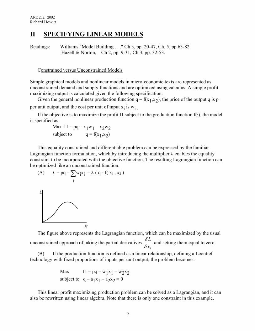
II SPECIFYING LINEAR MODELS Readings: Williams "Model Building . . ." Ch 3, pp. 20-47, Ch. 5, pp.63-82. Hazell & Norton, Ch 2, pp. 9-31, Ch 3, pp. 32-53. Constrained versus Unconstrained Models Simple graphical models and nonlinear models in micro-economic texts are represented as unconstrained demand and supply functions and are optimized using calculus. A simple profit maximizing output is calculated given the following specification. Given the general nonlinear production function q = f(x1,x2), the price of the output q is p per unit output, and the cost per unit of input xi is wi . If the objective is to maximize the profit Π subject to the production function f(·), the model is specified as: Max Π = pq – x1w1 – x2w2 subject to q = f(x1,x2) This equality constrained and differentiable problem can be expressed by the familiar Lagrangian function formulation, which by introducing the multiplier λ enables the equality constraint to be incorporated with the objective function. The resulting Lagrangian function can be optimized like an unconstrained function. (A) L = pq – ∑
i
wixi – λ ( q - f( x1 , x2 )
L
xi The figure above represents the Lagrangian function, which can be maximized by the usual
unconstrained approach of taking the partial derivatives δδLxi
and setting them equal to zero
(B) If the production function is defined as a linear relationship, defining a Leontief technology with fixed proportions of inputs per unit output, the problem becomes: Max Π = pq – w1x1 – w2x2 subject to q – a1x1 – a2x2 = 0 This linear profit maximizing production problem can be solved as a Lagrangian, and it can also be rewritten using linear algebra. Note that there is only one constraint in this example.
9

ARE 252. 2002 Richard Howitt
Max c'x subject to a'x = 0
where c p w wa a a' [ , , ]' [ , , ]= − −= − −
1 2
1 21 and the vector of input and output activities is: x ' = [ q, x1 , x2 ] Try multiplying this out to check that it is the same problem as above Linear Programming Linear Program: The equality constraint on the production function above is restrictive in that it implies that all the resources are exactly used up in the production processes. Given the nature of farm inputs such as land, labor, tractor time etc, inputs are available in certain quantities, but often they are not fully used up by the optimal production set. The relationship between the output levels q and the input levels x should be specified as inequality constraints for a more realistic and general specification. This inequality specification results in the Linear Program specification. Given a set of m inequality constraints in n variables ( x ), we want to find the non-negative values of a vector x which satisfies the constraints and maximizes some objective function.
EXAMPLE
Yolo County Farm Model In many places in this course we will use the following simple farm problem, based loosely on our local agriculture in Yolo County as a template to learn how linear programs are specified, solved and interpreted. We will use it for both analytical and empirical programming exercises.
The farm has the possibility of producing four different crops, alfalfa, wheat, corn and tomatoes. Yields are fixed so we can measure output by the number of acres of land allocated to each crop. The objective function is measured directly in net returns to the allocatable inputs. That is, the variable costs have been subtracted for simplicity. Constraints on production are all inequalities and represent the maximum amounts of land, water, and labor available, and a contract marketing constraint on the maximum quantity of tomatoes that the farmer can sell in any year. The resulting linear program can be written as follows: Maximize the scalar product of net returns c'x ( Remember that c is (n x 1) and x is also (nx1) Subject to the matrix of technical coefficients ( A ) and the vector of input resources available ( b ) Ax ≤ b where ( x ) is the vector of production or activity levels. The Yolo linear program is written as follows where the choice variables, measured in acres of land, are:
10

ARE 252. 2002 Richard Howitt
x1 = Alfalfa, x2 = Wheat, x3 = Corn, x4 = Tomato The Objective Function is measured in dollars or other money units and maximizes [ ]1 2 3121 160 135 825 4x x x+ + + x
Constraints
1
2
3
4
( ) 1.0 1.0 1.0 1.0 600.0( ) 4.5 2.5 3.5 3.25 1800.0( ) 6.0 4.2 5.6 14.0 5000.0
( ) 0.0 0.0 0.0 33.25 6000.0
xLand acrexWater ac ftxLabor hoursxContract tons
≤ − ≤
≤ ≤
The optimal solution is : x* =
0.0419.549
0.0180.451
We expect tomatoes to come into the profit maximizing solution since they have a high profit margin per unit of land. On one acre, we can grow 33.25 tons, but can only sell 6000 tons to the processor.
6000.033.25 /
tonstons acre
= a maximum acreage of 180.451 tomatoes. The rest of the land is used for the
next most profitable crop, wheat. This optimal solution is not short of either water or labor.
11
ARE 252. 2002 Richard Howitt
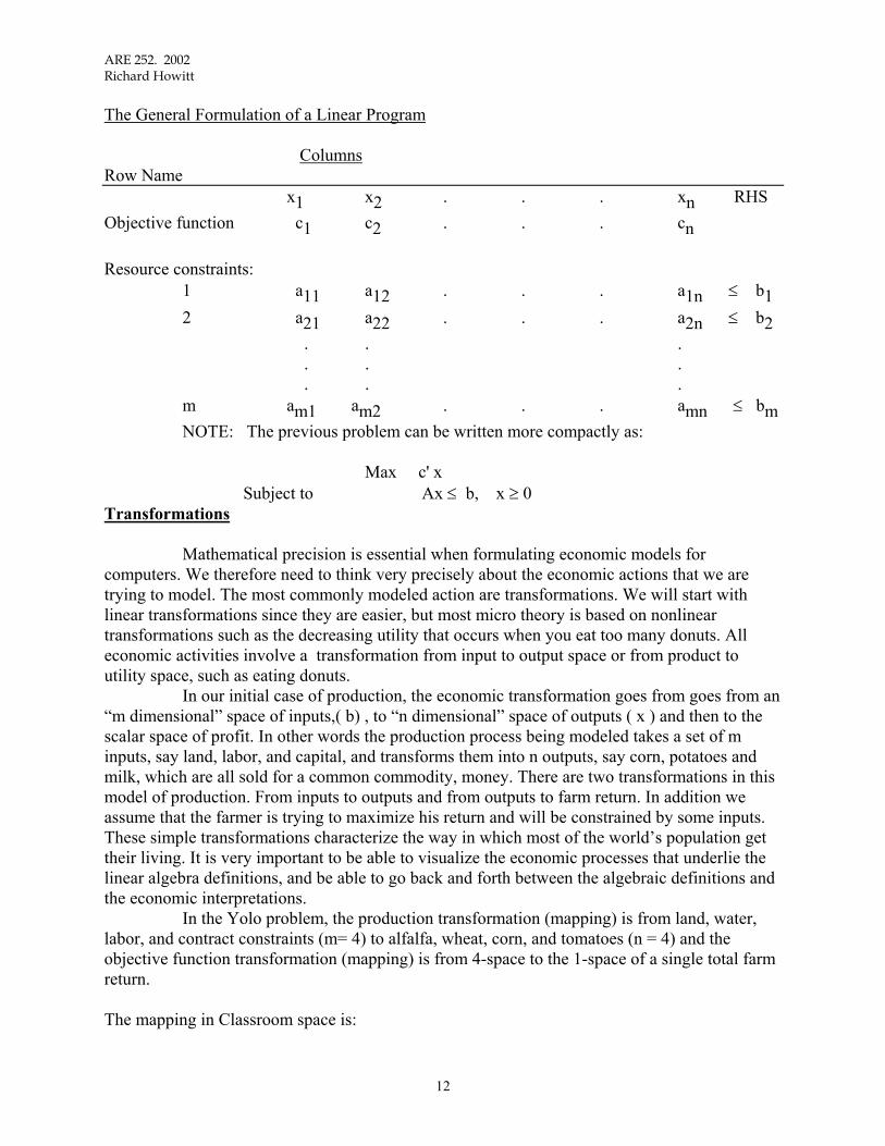
The General Formulation of a Linear Program Columns Row Name x1 x2 . . . xn RHS Objective function c1 c2 . . . cn Resource constraints: 1 a11 a12 . . . a1n ≤ b1 2 a21 a22 . . . a2n ≤ b2 . . . . . . . . . m am1 am2 . . . amn ≤ bm NOTE: The previous problem can be written more compactly as: Max c' x Subject to Ax ≤ b, x ≥ 0 Transformations Mathematical precision is essential when formulating economic models for computers. We therefore need to think very precisely about the economic actions that we are trying to model. The most commonly modeled action are transformations. We will start with linear transformations since they are easier, but most micro theory is based on nonlinear transformations such as the decreasing utility that occurs when you eat too many donuts. All economic activities involve a transformation from input to output space or from product to utility space, such as eating donuts. In our initial case of production, the economic transformation goes from goes from an “m dimensional” space of inputs,( b) , to “n dimensional” space of outputs ( x ) and then to the scalar space of profit. In other words the production process being modeled takes a set of m inputs, say land, labor, and capital, and transforms them into n outputs, say corn, potatoes and milk, which are all sold for a common commodity, money. There are two transformations in this model of production. From inputs to outputs and from outputs to farm return. In addition we assume that the farmer is trying to maximize his return and will be constrained by some inputs. These simple transformations characterize the way in which most of the world’s population get their living. It is very important to be able to visualize the economic processes that underlie the linear algebra definitions, and be able to go back and forth between the algebraic definitions and the economic interpretations. In the Yolo problem, the production transformation (mapping) is from land, water, labor, and contract constraints (m= 4) to alfalfa, wheat, corn, and tomatoes (n = 4) and the objective function transformation (mapping) is from 4-space to the 1-space of a single total farm return. The mapping in Classroom space is:
12
ARE 252. 2002 Richard Howitt
[ height, width, length] = scalar. The coordinates in 3 space locate a particular point on the
floor that is 6 ft from one wall and 12 ft from another.
1260
Other Examples of Production Transformations
Ford Cars [Capital, Labor, Steel, Energy] = [ Expedition, Eclipse ]
aaaa
CT
LT
ST
ET
aaaa
CE
LE
SE
EE
1 x 4 4 x 2 1 x 2
Candy [Sugar, Chocolate, Gum, Corn Syrup] = [ Milky Way Bar ] milkywayrecipe
1 x 4 4 x 1 1 x 1 Linear Algebra Definitions Used in Linear Programming
Definition: Linear transformation: A linear transformation T from n space to m space is a correspondence on the space En which maps each vector x in En into a vector T(x) in m-space. Transformations are performed by matrices or vectors as in the previous car or candy examples.
Note. Scalar multiplications can be carried through the linear transformation. That is, scalar multiplications can be factored out of the transformation as follows. Example. Given the vectors x1, x2, in, En, scalars λ1, λ2, and the transformation T(.)
T (λ1x1 + λ2x2) = λ1T(x1) + λ2T(x2).
Definition: Linear dependence: If a vector ai in a matrix A (mxn) can be expressed as a linear combination of the other vectors then it is linearly dependent. (informal, intuitive definition)
Given the vectors a1, . . ., am from the space En ,where m < n; The vectors ai are linearly dependent if there exist λi, i = 1, . . ., m s.t. λ1a1 + λ2a2 + . . . + λmam = 0 where not all the λi = 0. (math definition). It is sometimes easier to see the opposite case of linear independence. In this case, if the vectors
are linearly independent the only set of values for λi for which the linear transformation can be made to equal zero is when all the λi = 0 .
13
ARE 252. 2002Richard Howitt
14
An Example of Linear DependenceSet λ1 = 1.
From the definition of linear dependence, λ1a1 + λ2a2 + . . . + λmam = 0 ,
Therefore setting λ1 = 1. λ2a2 + . . . + λmam = -a1since a1 is not = 0, then some λi, i = 2 . . . m, must also be non zero.
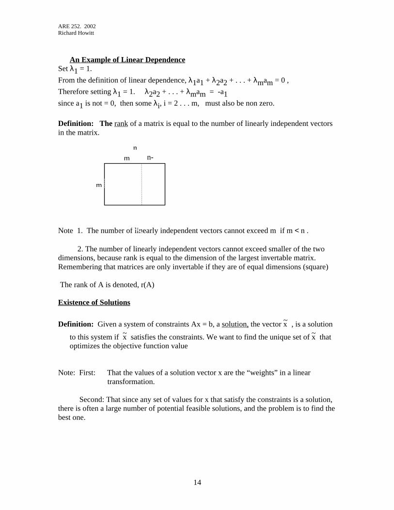
Definition: The rank of a matrix is equal to the number of linearly independent vectorsin the matrix.
Note 1. The number of linearly independent vectors cannot exceed m if m < n .
2. The number of linearly independent vectors cannot exceed smaller of the twodimensions, because rank is equal to the dimension of the largest invertable matrix.Remembering that matrices are only invertable if they are of equal dimensions (square)
The rank of A is denoted, r(A)
Existence of Solutions
Definition: Given a system of constraints Ax = b, a solution, the vector x~ , is a solution
to this system if x~ satisfies the constraints. We want to find the unique set of x~ thatoptimizes the objective function value
Note: First: That the values of a solution vector x are the “weights” in a lineartransformation.
Second: That since any set of values for x that satisfy the constraints is a solution,there is often a large number of potential feasible solutions, and the problem is to find thebest one.
nm
m
n-

ARE 252. 2002 Richard Howitt
A Homogenous System A system is defined as Homogeneous if all the values for the right hand side are zero (Ax = 0,) In other words, b is defined as zero. Homogenous systems are often used as they are simpler to represent and manipulate. The trivial solution of x = 0 always exists. Non-homogenous systems can always be converted to homogenous systems by matrix augmentation.
Note We can convert Ax = b to A x = 0, where A = Ab the "augmented matrix"
and x =
x
-1 the augmented vector
EXAMPLE
A =
a11 a12
a21 a22 b =
b1
b2 x =
x1
x2
In the example above Ax = b, alternatively we can write the same equations in the form of Ax – b = 0.
a11 a12 b1
a21 a22 b2
x1
x2
-1
=
0
0
or redefining the matrices and vectors it equals A x =
0
Case 1. No Solution to the System Exists No solutions exist to Ax = b if the rank of A (r(A)) is less than the rank of the augmented matrix where is defined as the augmented matrix [Ab]. Here we compare the rank for the augemtned and unaugmented matrices.
$A $A
The rank condition where r( ) > r (A ) means that there are no solutions ( except the trivial solution) since b is linearly independent of A.
$A
Note that b must be linearly independent of all the vectors in A if augmenting A by b increases the rank of over the rank of A . $AFrom the definition of a solution as a linear transformation, the linear independence of B from every vector in A means that no solutions can exist. In other words, the only set of weights
(allocations) that can make A x = 0 is the trivial solution when every value in = 0. x x
15
ARE 252. 2002 Richard Howitt
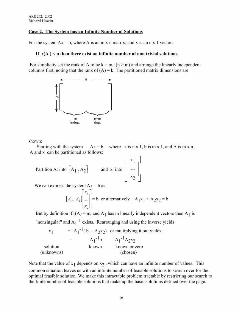
Case 2. The System has an Infinite Number of Solutions For the system Ax = b, where A is an m x n matrix, and x is an n x 1 vector. If r(A ) < n then there exist an infinite number of non trivial solutions. For simplicity set the rank of A to be k = m, (n > m) and arrange the linearly independent columns first, noting that the rank of (A) = k. The partitioned matrix dimensions are
shown:
n
m
m indep.
n–m dep.
Starting with the system Ax = b, where x is n x 1, b is m x 1, and A is m x n , A and x can be partitioned as follows:
Partition A: into A1 ... A2 and x into
x1
---x2
We can express the system Ax = b as:
= b or alternatively A1x1 + A2x2 = b [ ]
2
1
21 ........x
xAA
But by definition if r(A) = m, and A1 has m linearly independent vectors then A1 is
"nonsingular" and A1-1 exists. Rearranging and using the inverse yields
x1 = A1-1( b – A2x2) or multiplying it out yields:
= A1-1b – A1
-1A2x2 solution known known or zero (unknowns) (chosen) Note that the value of x1 depends on x2 , which can have an infinite number of values. This common situation leaves us with an infinite number of feasible solutions to search over for the optimal feasible solution. We make this intractable problem tractable by restricting our search to the finite number of feasible solutions that make up the basic solutions defined over the page.
16
ARE 252. 2002 Richard Howitt
Case 3. A Unique Solution Exists to the System The system Ax = b has a unique solution if: ( 1 ) r( A ) = r( Ab ) That is, the RHS augmented matrix has the same rank as A (2 ) The matrix A is square and of full rank. That is, A = m x m and r( A ) = m SUMMARY Solutions to the set of equations Ax = b have the following conditions: ( a ) r ( A ) < r (Ab ) No Solution ( b ) r ( A ) < dim ( x ) Infinite Number of Solutions ( c ) r ( A ) = dim (x ) Unique Solution and A is full rank Basic Solutions Definition: Given Ax = b, A is m x n, r(A) = m, A basic solution to the system is when (n – m) predetermined values of x (x 2 ) are set = 0. Using the previous example, set x2 = 0. The basic solution is x1 = A1
-1b For convenience define A1, as B, and A2 as D. We can now write the system as:
xB = B-1b where x1 is denoted xB, and x2 (set =0) is denoted xD
Note 1. That since B is m x m and non-singular, the inverse B-1 exists Note 2. Given that there are (n-m) non basis vectors, there are many, but a finite number of
alternative basic solutions. Definition: Basic Feasible Solution (B.F.S.) A basic feasible solution x is defined as: Basic Solutions x such that x = B-1b,
17

ARE 252. 2002 Richard Howitt
and Feasible x ≥ 0. That is: a basic feasible solution that has non-negative values for the basic solution vectors. A basic feasible solution where the x values in the basis are defined as all positive. Definition: Convex Sets: A set X is convex if for any points x1 and x2 ⊆ X, the line
segment x1,x2 is also ⊆ X, i.e., "The set X is convex if: There exist x1,x2 ⊆ X, such that the linear combination λx1 + (1 – λ)x2 is also contained in X, for 0 ≤ λ ≤ 1" This last line is interpreted as “ anywhere on a line between x1 and x2” Note that λx1 + (1 – λ)x2 is by definition a convex linear combination
x2
1x
λ = 0 implies that we are at point x2 λ = 1/2 implies a point half way between x1 and x2 λ = 1 implies point x1
Intuition: Sets with holes or dents are not convex.
x2
1x
Definition: The Extreme Point of a convex set is x if x ⊆ X, but there do not exist any other x– 1, x– 2 ⊆ X such that x = λx– 1 + (1 – λ)x– 2 for 0 < λ < 1. What this says that an extreme point is a member of the set, but it cannot be expressed as a linear combination of any other points in the set. For an enjoyable empirical example, visit the lighthouse on the furthest west point of Point Reyes State park. NOTE ( 1) In this definition λ is strictly <, not ≤ ( 2) Any point that satisfies the definition above is a single point, because it is in the set,
but only at an extreme point. ( 3 ) Intuitively, an extreme point of a convex set is part of the convex set, but cannot be expressed as a linear combination of any other two points in the convex set.
18

ARE 252. 2002 Richard Howitt
1x
In a linear system an infinite number of solutions often exist, the objective function is used to select the maximum or minimum value. However to reduce the number of values to search for optimal value we use the properties of the basic feasible solution to reduce the search problem to one over a finite set of possible optimal values. Basic feasible solutions are the non-negative extreme points.
The number of extreme points of a linear constraint set is finite. Accordingly, if we search the set of basic feasible solutions for the optimal value of the objective function, we will have found the optimal for the whole set. Note that if the constraints are nonlinear, the resulting convex set now has an infinite number of solutions again. To solve for the optimum in this case we have to use a different approach that is addressed later in the course. Slack or Surplus Variables Slack or surplus variables in a linear program are use to convert the inequality constraints into equality constraints, thus making the problem easier to write mathematically and helping the interpretation of the model. They are some times called "artificial variables". While you have to understand the interpretation of these variables, in actual LP models they are usually put in automatically by the computer algorithm. The two types of artificial variable correspond to the two types of inequality constraint. “Less than” ( ≤ ) constraints are converted to equality constraints by Slack variables, while “Greater than” ( ≥ ) constraints require Surplus variables. Intuitively, if an inequality constraint may or may not be binding, but you want to always express it mathematically as a binding constraint there will be slack input to dispose of if the constraint is a “less than” ( ≤ ) or a surplus to use up if the constraint is a “greater than” ( ≥ ).
19

ARE 252. 2002 Richard Howitt
Example of a Slack variable in the Yolo model land constraint. Alfalfa Wheat Corn Tomato Slack Land Land 1 1 1 1 1 = 600 Note: 1. Objective function values of slack/surplus variables are zero. 2. Computer puts them in automatically (in GAMS). 3. Gives us an initial basic feasible solution for the simplex method to use. 4. The initial solution is:
(a) Guaranteed basic due to the diagonal constraint matrix (b) Guaranteed feasible by the non-negativity condition on slack/surplus variables (c) Won't add to the objective function value as they have zero objective function
values Surplus variables ( for ≥ constraints) have a negative signed coefficient in the constraint because we want to reduce the surplus above the right hand side value, and thus reformulate the constraint as an equality. Linear Program Objective Function Specification- Traditional Normative Approach Economic Properties of Linear Program Objective Functions Linearity of the objective function in the parameters (Max c'x where c = the parameters) Constant Returns to Scale, i.e., cost/unit production is constant. Constant output prices (price-taker) (no regions, nations or large firms). Some common examples of objectives are: Maximization of profit (Neoclassical Firm objective ) Minimizing deviations from central planning targets Minimizing costs in a planned economy Minimizing risk of starving next season Note: The units in the objective function are usually defined by the price units, for example $ per ton. In the constraint matrix it is essential that there is consistency between the constraint units and objective function units. EXAMPLE Yolo Farm problem. No costs are specified in the Yolo problem. The objective function parameters are "Gross margins / acre." which are based on primary data and are equal to total revenue / acre – variable costs / acre.
20
ARE 252. 2002 Richard Howitt
This simple objective function specification works well until we need to consider capital investments, or changes in production technology as part of the problem to be solved. If changes in the amount of input used is part of the problem to be optimized then the net return per acre will change which requires a more complicated specification.
Specifying Linear Constraints Types of Constraints Linear constraints can be classified into three broad classes. (a) Resource Constraints In most linear models of production or distribution, resource constraints are intuitive.
They usually take the form of a set of “m” summation constraints over the “n” activities. This form assumes that there are n possible production activities and m possible fixed resources used by the activities. The fixed resources are available in quantities b1… bm.
The standard specification of this form is Max c′x subject to Ax ≤ b The matrix A has individual elements, which are the input requirement coefficients for the
production activities. (b) Bounds Where there are institutional limits on the activity levels, or because of bounds on the
range of the linearity assumption, we may wish to bound the individual activity values. Bounds can be specified using a single row for each bounded activity. The general "less than or equal to" form of constraint can be used in the following way:
Ix ≤ b where the values for the b vector components bi are the levels of the upper or lower bounds.
Upper bounds have positive values for bi . Lower bounds have negative values on both bi and the corresponding 1 value in the identity matrix.
21

ARE 252. 2002Richard Howitt
22
(c) Linkage Constraints
This type of constraint links two or more activities in a prespecified manner. Themost common use of linkage constraints is to sum up total output or input use by activities.This operation is often needed where the total input use must be held in storage or purchasedfrom another economic unit. Another common specification is an inventory equation thatkeeps track of commodity levels used, produced and on hand in the model. The units in thelinkage constraint row usually determine the coefficients corresponding to each activity.
Linkage constraints are best approached systematically
(1) Decide on the best units for the constraint row.(2) Write out the logic of the constraint in words. For example, a hay inventory rowshould be specified in tons. If the activities influencing the row are.
(i) Hay grown (acres)(ii) Cattle to be fed (head)(iii) Hay bought (tons)(iv) Hay on hand in storage (tons)
Constraint logic – "Hay consumed by cows plus the change in storage equals hay grownplus hay purchased." The easiest way to think of linkage constraints is to define the"Flows in" and "Flows out" of the coomodity that the constraint defines. Then decide ifthe problem requires that the flows in are greater than, less than, or equal to the flows out.
(3) Although linkage constraints are usually equalities, LP problems solve more easily ifthe constraints are specified as inequalities. The trick is to specify the signs of thecoefficients so that the constraint is driven to hold as an equality by the objectivefunction. For example if a constraint is set as a “greater than” inequality that requires abasic ration for animal production but allows a greater amount of food to be fed. Anoptimizing model will always constrain the ration to the basic level if the food input iscostly or constrained.
Example 1Maximizing net revenue. Three output activities x1, x2 , x3.
All activities require different quantities of a variableinput x4, with aij input requirement coefficients of : a41, a42, a43.
Objective Row c1 c2 c3 –c4Linkage Row a41 a42 a43 –1 ≤ 0.
The row is measured in units of the variable input x4. The cost per unit is c4. The linkage row
above allows the possibility that more x4 can be purchased than is needed by production

ARE 252. 2002 Richard Howitt
activities x1, x2 and x3. However, since the extra units have a cost associated with them the objective function will be reduced by the “slack” activities and hence an optimizing model will not purchase more input than is needed. The linkage row does require that the units of x4 required by the production of x1, x2 and x3 are summed and that this sum is less than or equal to x4. In short, you can buy too much x4, but you cannot buy too little.
(4) If the problem solution is unbounded, check the signs in the constraint.
(5) Check the operation of the linkage constraint by hand calculations on a
representative constraint at the optimal solution values.
(6) Inventory stocks can be incorporated most simply by right hand side values, (example 2). An alternative approach is to specify a separate column for the inventory
stock activity, which may itself be constrained by upper or lower bounds (example 3). This approach is required if the stock is priced as a separate activity in the objective function.
Example 2 A stock of 50 units of x4 is available at the start of the problem.
Objective Row c1 c2 c3 –c4 Linkage Row a41 a42 a43 –1 ≤ 50. The resulting constraint in the optimal solution will have the form: x1 a41 + x2 a42 + x3 a43 - x4 ≤ 50. The interpretation is that the model has to satisfy the requirements of activities x1 .. x3 by using some of the unpriced 50 units on hand, or they can buy inputs for a price c4 through activity x4. Example 3
The problem starts with no stocks of x4, but is required to have 100 units in stock at the optimal solution. We now specify activity x5 as the stock of input x4, for instance hay. Activity x4 is defined as purchasing or growing hay.
Objective Row c1 c2 c3 –c4 c5
Linkage Row a41 a42 a43 –1 1 ≤ 0 Minimum Stock Row –1 ≤ -100.
23
ARE 252. 2002 Richard Howitt
Models of Transportation Problems Linear optimization is particularly good at solving problems that minimize the cost of transporting a commodity from defined sources to destinations. If there are:
n sources defined by i = 1 …. n m destinations defined by j = 1 … m, Note- there are n times m possible ways to transport the commodity. The activity ( the amount shipped ) is therefore defined as xij and has an associated cost
of transport of cij. The objective function is therefore to Minimize z = Σi Σj cij xij Demand at destinations. The transport problem is constrained by a set of minimum demand quantities at each destination. If the quantity demanded at destination j is defined as bj the demand constraint is : Σi xij ≥ bj It says “ the sum of the amounts that arrive from all sources must be greater or equal to ( ≥ ) the amount demanded at destination j” Source “Supply” Constraints The total amount shipped out of any supply source cannot exceed its capacity. Given a maximum capacity of ai at source i , the supply constraint is : Σj xij ≤ ai It says “The amount shipped from source i to all destinations must be less than or equal to (≤ ) the
amount available at source i”.
The complete transportation problem for n sources ( i = 1…n) and m destinations (j = 1…m) is:
Minimize Total Cost z = Σi Σj cij xij
subject to Σj xij ≤ ai Σi xij ≥ bj
24

ARE 252. 2002 Richard Howitt
25
Demand Shortage Costs and Transportation Cost Often problems can be written more realistically by redefining the demand constraints as not having to hold exactly, but to incur “Shortage Costs” if they are not met. To influence the optimal solution, the outage costs of not having enough product must exceed the transportation and supply costs. Outage activities are included in the left-hand side of the demand constraints. Σi xij + outj ≥ bj Given an shortage cost of "coutj" , the transportation model objective function is now Σi Σj cij x ij + Σj coutj out j The model now finds the optimum pattern of transportation for the supplies on hand, and calculates the cost minimizing way to spread the shortage among destinations.

ARE 252 2002 Richard Howitt
III SOLVING LINEAR MODELS Solution Sets A linear equality constraint defines a line in two space, a plane if it is in three space, and a hyperplane if the constraint is in n dimensions. It follows that a linear constraint (inequality) in “n space”divides the space into two half spaces. Therefore the set of values that satisfy several linear constraints must be common to (or contained in) the intersection of several half-spaces. Fortunately it turns out that the intersection of linear half-spaces is a convex set. Therefore the set of possible solutions which can satisfy several linear constraints at the same time is a convex set. This convex set is known as the feasible solution set for the linear inequality constraints, since any point in this set can satisfy all the constraints. We use the properties of convex sets to search over the large set of possible solutions in an efficient way for the optimal solution that maximizes some particular objective. The Fundamental Theorem of Linear Programming Given a linear programming problem in the usual matrix algebra form: max c'x subject to. Ax ≤ b where A is m x n with rank (A) = m: The Theorem can be summarized by stating that: 1. If a feasible solution exists to the problem, a basic feasible solution to the problem also exists. 2. If an optimal feasible solution exists, then an optimal basic feasible solution to the problem also exists. Therefore all we have to do is check which of the basic feasible solutions maximizes the objective function and we know that we have checked all the possible candidates for the optimal basic feasible solution. EXAMPLE Given the following set of inequality constraints: x1 ≤ 5 3x1 + 5x2 ≤ 30 x1 , x2 ≥ 0 We can show these inequality constraints graphically in x1 , x2 space.
26

ARE 252 2002 Richard Howitt
X1 ≤ 5
3x1 + 5x2 ≤ 30
6
X2
5 10 X1 The intersection of the two half-spaces is the feasible solution space. Note that the feasible solution set is a convex set with four extreme points at each corner. Extreme Points and Basic Solutions Given system Ax = b, x ≥ 0 where A is m x n, and the rank of A, r(A) = m: If K is the convex set of all solutions to the system (i.e., the set of possible (n x 1)
vectors x that satisfy the system). Then a vector x is an extreme point of K if x is a basic solution to the system. Definition: A Basic solution: is defined as a solution where all the basic variables are
non-zero, all other non-basic variables are zero. Corollary: If a feasible solution exists then there exist a finite number of potentially optimal solutions. Given that we can be sure that our optimal solution is among the basic feasible
solutions we can now concentrate the search for optimal solutions among the finite set of basic solutions. Note that for the feasible solution set, the number of extreme points equals the numbers of binding constraints which also equals the number of non-zero basis activities.
27

ARE 252 2002Richard Howitt
28
An Introduction to the Simplex AlgorithmThe Simplex algorithm
An algorithm is a set of systematic instructions to the computer that enables us toprogram it to perform a given task.. The Simplex algorithm is one of the oldest but still thebest algorithm for most problems of linear optimization. Its operation can be summarized as:
1 – Changing the basis of the problem, and hence the solution, by changing basis vectors
2 – Using the objective function value for a systematic choice of basis vectors that always improve the objective function.
Since the algorithm is driven by the effect of a change of basis on the objective function, tounderstand its operation we need to analyze the algebra and economics of a change of basis forthe following familiar LP problem.
Max Π = c'x s.t. Ax = b, x ≤ 0, A is m x n, and rank A = m.
Partition A into basis and non-basis matrices denoted respectively B and D. Defining the partition of A ≡ [B D]
↑ ↑ basis non-basis m x m m x (n–m)
when partitioned, x and c' become: x =
xB
---
xD
c' = c 'B ... c 'D
The L.P. problem becomes: max c 'B ... c 'D
xB
---
xD
s.t. B ... D
xB
---
xD
≤ b
or multiplying out the partitioned matrices results in: Max Π = c 'B xB + c 'D xD s.t. BxB + DxD ≤ b
xB ≥ 0, xD ≥ 0
An optimal basic feasible solution (BFS) has the elements of xB are all non-zero
(assuming non-degenerate solutions, dealt with later), and all the xD elements are zero. The
constraints for a basic feasible solution become:

ARE 252 2002 Richard Howitt
BxB + D [0] = b or more concisely, Bx
B = b
Since B-1 exists by definition of a basis (m x m, m linearly independent rows) A basic feasible solution to the system is: xB = B-1 b However the point of this analysis is to find the effect of a change of the basic solution on the value of the objective function. Accordingly, the partitioned x vector is used to write the objective function in terms of basis and non basis variables. The partitioned objective function is B B Dc x c xD′ ′Π = + or substituting in the solution above: 1 sin 0B D Dc B b c x ce x−′ ′Π = + =D
For basic solutions the objective function is: Π = 1
Bc B b−′ What happens to the objective function value (z) when we consider introducing one
of the xD (non basis vectors), say "xj" into the basis? The analogy is the “In group” and “Out group” in US High schools where teenage popularity is very important. One way in which one can judge and be judged as to what group you are in is with whom you eat lunch. Assume for mathematical reasons that the lunch bench has a finite dimension ( the rank of the basis matrix) and the number of people who can sit on the bench is limited. Since teenage popularity is fickle, it is quite likely that individuals (vectors) move in and out of the “In group” over time. The point is that if a new individual is popular enough to be admitted to the “In group”, someone will have to leave the bench ( the basis ) and the other members of the group will have to rearrange their seating on the bench with the arrival of the new entrant. Mathematically this process can be represented as:
Problem: Those who stay have to move over, and someone (a vector) will have to leave the basis. Writing out a solution to the partitioned constraints yields: Bx
B + Dx
D = b subtracting the non basis values
Bx
B = b – Dx
D premultiplying by B-1 x
B = B-1b – B-1Dx
D Now we substitute this result into the objective function to see the effect of the introduction of a non-basis activity into the basis. This changes the objective function value. Since Π = c′Bx
B + c′Dx
D substituting in for xB from above yields:
29
ARE 252 2002 Richard Howitt
= c′B )11DDxBbB −− −( + c′Dx
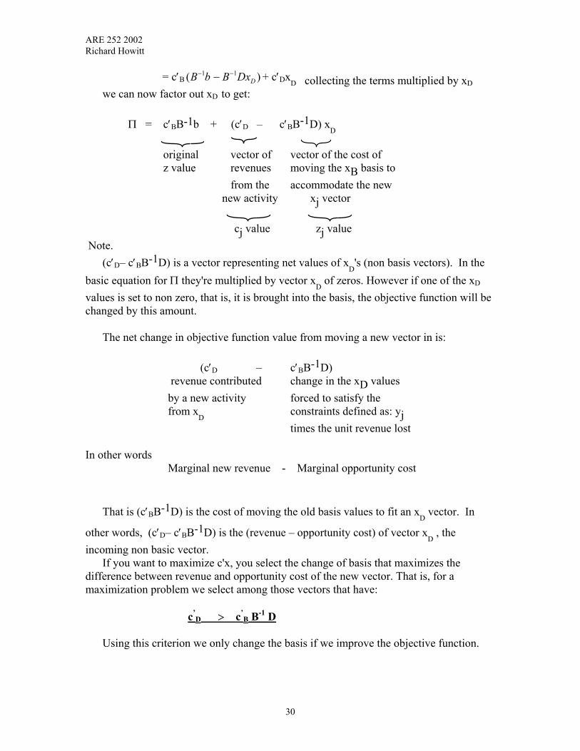
D collecting the terms multiplied by xD we can now factor out xD to get: Π = c′BB-1b + (c′D – c′BB-1D) x
D
original vector of vector of the cost of
z value revenues moving the xB basis to from the accommodate the new new activity xj vector
cj value zj value Note.
(c′D– c′BB-1D) is a vector representing net values of xD's (non basis vectors). In the
basic equation for Π they're multiplied by vector xD of zeros. However if one of the xD
values is set to non zero, that is, it is brought into the basis, the objective function will be changed by this amount. The net change in objective function value from moving a new vector in is: (c′D – c′BB-1D) revenue contributed change in the xD values by a new activity forced to satisfy the from x
D constraints defined as: yj times the unit revenue lost In other words Marginal new revenue - Marginal opportunity cost That is (c′BB-1D) is the cost of moving the old basis values to fit an x
D vector. In
other words, (c′D– c′BB-1D) is the (revenue – opportunity cost) of vector xD , the
incoming non basic vector. If you want to maximize c'x, you select the change of basis that maximizes the difference between revenue and opportunity cost of the new vector. That is, for a maximization problem we select among those vectors that have: c’
D > c’B B-1 D
Using this criterion we only change the basis if we improve the objective function.
30
ARE 252 2002 Richard Howitt
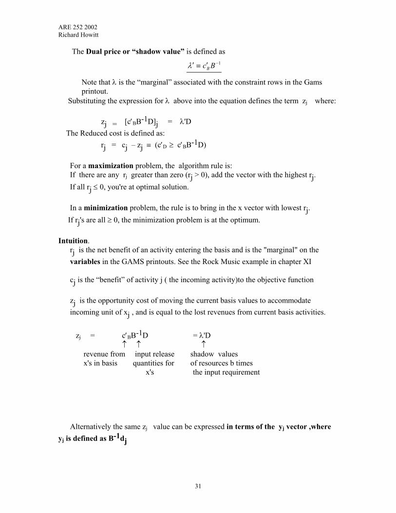
The Dual price or “shadow value” is defined as 1−′≡′ BcBλ
Note that λ is the “marginal” associated with the constraint rows in the Gams printout. Substituting the expression for λ above into the equation defines the term zj where: zj = [c′BB-1D]j = λ'D The Reduced cost is defined as: rj = cj – zj ≡ (c′D ≥ c′BB-1D) For a maximization problem, the algorithm rule is: If there are any rj greater than zero (rj > 0), add the vector with the highest rj. If all rj ≤ 0, you're at optimal solution. In a minimization problem, the rule is to bring in the x vector with lowest rj. If rj's are all ≥ 0, the minimization problem is at the optimum. Intuition. rj is the net benefit of an activity entering the basis and is the "marginal" on the variables in the GAMS printouts. See the Rock Music example in chapter XI cj is the “benefit” of activity j ( the incoming activity)to the objective function zj is the opportunity cost of moving the current basis values to accommodate incoming unit of xj , and is equal to the lost revenues from current basis activities. zj = c′BB-1D = λ'D ↑ ↑ ↑ revenue from input release shadow values x's in basis quantities for of resources b times x's the input requirement Alternatively the same zj value can be expressed in terms of the yj vector ,where yj is defined as B-1dj
31
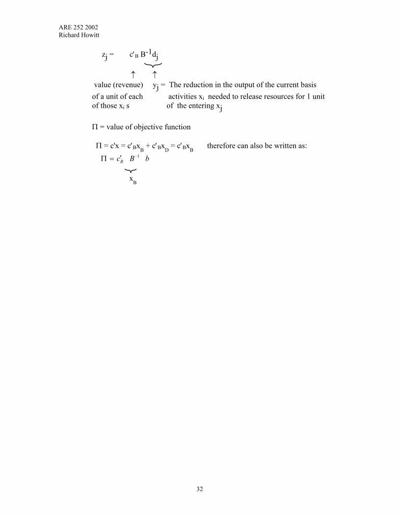
ARE 252 2002 Richard Howitt
zj = c′B B-1dj ↑ ↑ value (revenue) yj = The reduction in the output of the current basis of a unit of each activities xi needed to release resources for 1 unit of those xi s of the entering xj Π = value of objective function Π = c'x = c′Bx
B + c′Bx
D = c′Bx
B therefore can also be written as:
1Bc B b−′Π =
x
B
32
ARE 252 2002 Richard Howitt
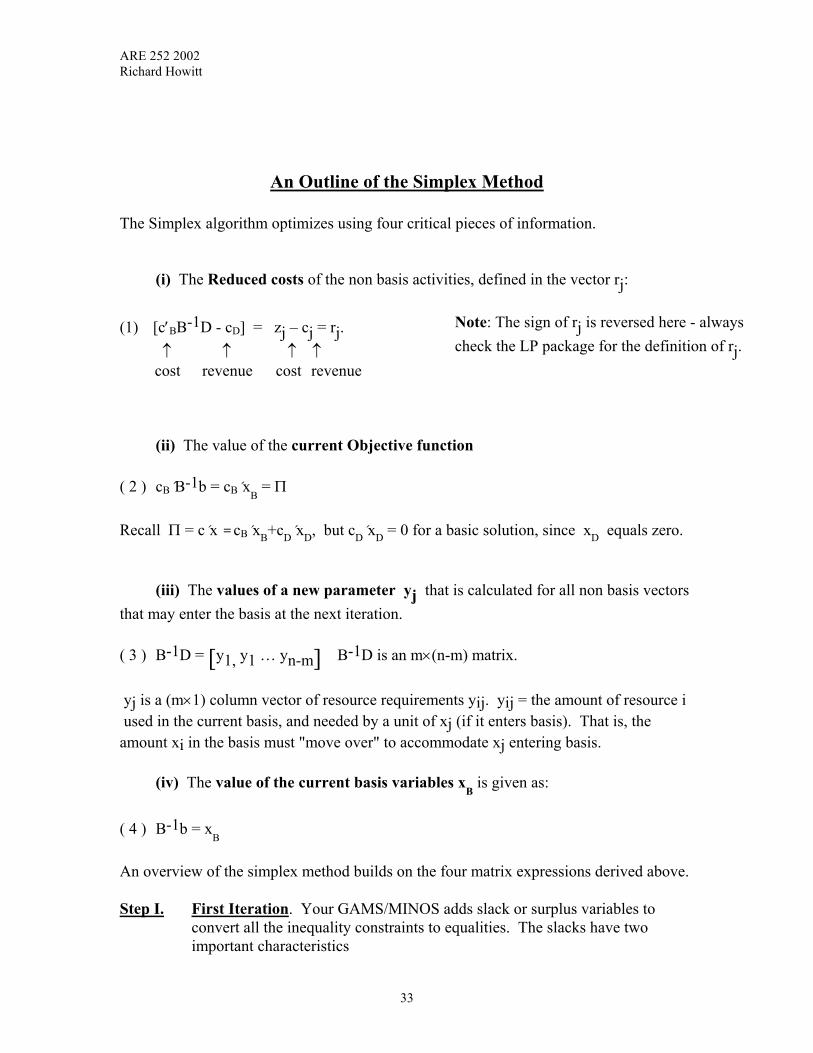
An Outline of the Simplex Method
The Simplex algorithm optimizes using four critical pieces of information. (i) The Reduced costs of the non basis activities, defined in the vector rj: (1) [c′BB-1D - cD] = zj – cj = rj. ↑ ↑ ↑ ↑ cost revenue cost revenue
Note: The sign of rj is reversed here - always check the LP package for the definition of rj.
(ii) The value of the current Objective function ( 2 ) cB´B-1b = cB´x
B = Π
Recall Π = c´x = cB´xB+cD´xD, but cD´xD = 0 for a basic solution, since xD equals zero. (iii) The values of a new parameter yj that is calculated for all non basis vectors that may enter the basis at the next iteration. ( 3 ) B-1D = [ ]y1, y1 … yn-m B-1D is an m×(n-m) matrix. yj is a (m×1) column vector of resource requirements yij. yij = the amount of resource i used in the current basis, and needed by a unit of xj (if it enters basis). That is, the amount xi in the basis must "move over" to accommodate xj entering basis. (iv) The value of the current basis variables x
B is given as:
( 4 ) B-1b = x
B
An overview of the simplex method builds on the four matrix expressions derived above. Step I. First Iteration. Your GAMS/MINOS adds slack or surplus variables to
convert all the inequality constraints to equalities. The slacks have two important characteristics
33

ARE 252 2002 Richard Howitt
( i ) Zero values in the objective function coefficient row (c) (ii) A constraint matrix which is an identity matrix. Thus, an initial basis of all slack and surplus variables is always ( i ) Of full rank (ii) Feasible (iii) Zero value objective function and therefore, zero opportunity costs zj for
alternative activities. Step II. For each xj not in the basis calculate the reduced cost rj = ( cj – zj ), which
is the net benefit of xj entering the basis. (For the first iteration, rj = cj). Select the xj with maximum rj > 0 to enter the basis. (For a maximization problem).
For a maximization problem - if any rj > 0, the problem is not optimal,
therefore, select the maximum rj > 0 to enter the basis. Step III. The yj vector is used to select the activity that leaves the basis. yj is an m x 1 vector of values that show the rate of substitution between the
basis activities xBi and the incoming vector xk chosen in step II From equation ( 3 ) we see that B-1D yields (n – m) "yj" vectors, each with m
elements. If we pick a non basis vector in D, say dk, to enter the basis, the corresponding yk vector will be:
( 5 ) yk = B-1dk = B-1ak Using ( 5 ) we can also write ak - the input requirements for the incoming vector- as a function of yk: ( 6 ) ak = Byk But since B is the basis submatrix of A, ( 7 ) B = [a1, a1, . . ., am] and thus from ( 7 ) the potential incoming vector ak selected in step II can be expressed as a linear combination of the basis vectors. Substituting ( 7 ) back into ( 6 ) yields: ( 8 ) ak = a1 y1k + a2 y2k + . . . + am ymk we can also multiply each element in ( 8 ) by an arbitrary nonzero scalar ε
34

ARE 252 2002 Richard Howitt
( 9 ) εak = a1 ε y1k + a2 ε y2k + . . . + am ε ymk Expanding the basic feasible solution BxB = b using ( 7 ) for B results in. (10) a1 x1 + a2 x2 + . . . + am xm = b We now introduce –εak and εak into the feasible basis in equation (10). Note (1) If ε ≡ 0, no basis change occurs. (2) The algebraic trick of adding and subtracting within an identity (11) a1 x1 + a2 x2 + . . . + am xm –εak + εak = b Multiplying ( 9 ) by -1 and substituting the right hand side of ( 9 ) into (11) for –εak yields (12) a1 x1 + a2 x2 + . . . + am xm + –a1 εy1k – a2 εy2k . . . –am εymk + εak = b factoring out the a1, . . ., am vectors gives ( 13 ) a1(x1–εy1k) + a2(x2–εy2k) + . . . + am(xm–εymk) + εak = b. Point. As we increase the value of the scalar ε, the influence of ak increases, and (xi – εyik) will be driven to zero for some activity i. This activity will leave the basis. Note 1. That by the definition of a basic solution, when an activity is driven to a zero value it leaves the basis. 2. An m + 1 dimensional object in m dimensional space is called a SIMPLEX, hence the name of this algorithm.
3.The first term to be driven to zero will have the smallest xi/ yik since (xi – εyik) = 0 when ε = xi/ yik .
From ( 13 ) we can see two outcomes of changes in the value of ε:
1. If ε = 0 we get the old basis in ( 7 ) 2. If ε is made large, the importance of the new vector ak increases, but there is a
danger that one of the new variable values (xi – εyik) will be driven to a negative value, which would produce an infeasible solution.
35
ARE 252 2002 Richard Howitt
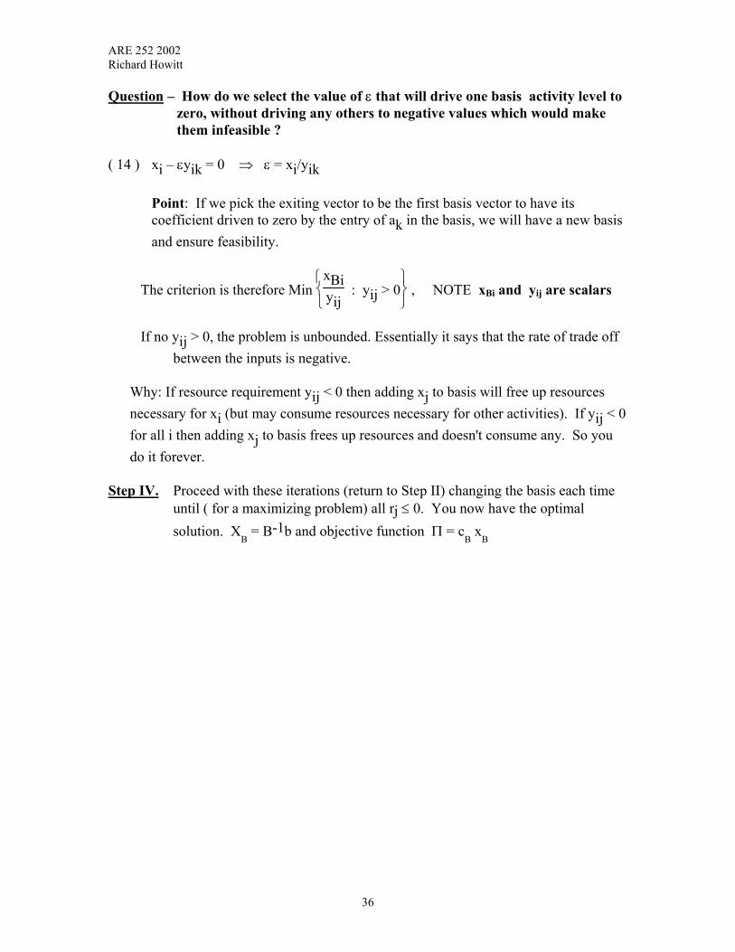
Question – How do we select the value of ε that will drive one basis activity level to zero, without driving any others to negative values which would make them infeasible ? ( 14 ) xi – εyik = 0 ⇒ ε = xi/yik
Point: If we pick the exiting vector to be the first basis vector to have its coefficient driven to zero by the entry of ak in the basis, we will have a new basis and ensure feasibility.
The criterion is therefore Min
xBi
yij : yij > 0 , NOTE xBi and yij are scalars
If no yij > 0, the problem is unbounded. Essentially it says that the rate of trade off
between the inputs is negative. Why: If resource requirement yij < 0 then adding xj to basis will free up resources
necessary for xi (but may consume resources necessary for other activities). If yij < 0 for all i then adding xj to basis frees up resources and doesn't consume any. So you do it forever.
Step IV. Proceed with these iterations (return to Step II) changing the basis each time
until ( for a maximizing problem) all rj ≤ 0. You now have the optimal solution. X
B = B-1b and objective function Π = c
B xB
36
ARE 252 2002 Richard Howitt
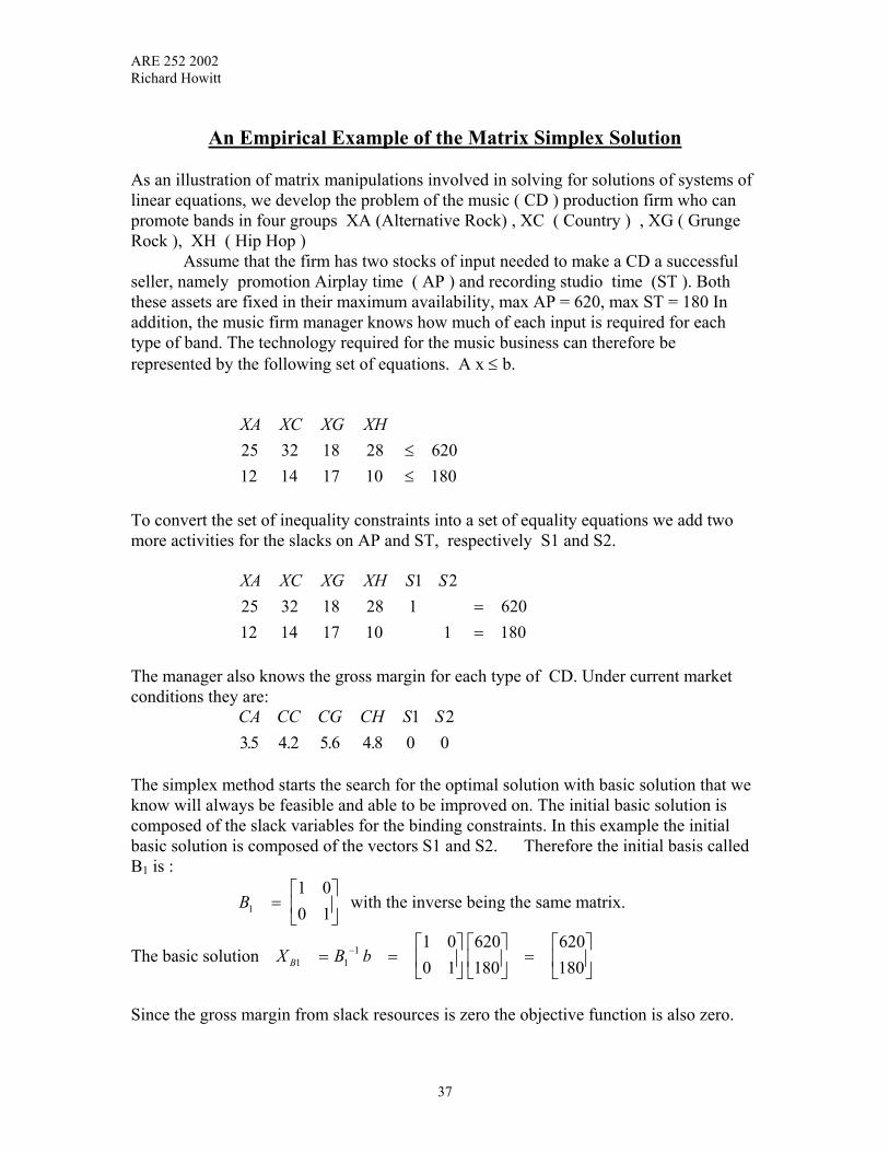
An Empirical Example of the Matrix Simplex Solution
As an illustration of matrix manipulations involved in solving for solutions of systems of linear equations, we develop the problem of the music ( CD ) production firm who can promote bands in four groups XA (Alternative Rock) , XC ( Country ) , XG ( Grunge Rock ), XH ( Hip Hop ) Assume that the firm has two stocks of input needed to make a CD a successful seller, namely promotion Airplay time ( AP ) and recording studio time (ST ). Both these assets are fixed in their maximum availability, max AP = 620, max ST = 180 In addition, the music firm manager knows how much of each input is required for each type of band. The technology required for the music business can therefore be represented by the following set of equations. A x ≤ b.
XA XC XG XH2512
3214
1817
2810
620180
≤≤
To convert the set of inequality constraints into a set of equality equations we add two more activities for the slacks on AP and ST, respectively S1 and S2.
XA XC XG XH S S2512
3214
1817
2810
11
2
1620180
==
The manager also knows the gross margin for each type of CD. Under current market conditions they are:
CA CC CG CH S S35 4 2 5 6 4 8
1 20 0. . . .
The simplex method starts the search for the optimal solution with basic solution that we know will always be feasible and able to be improved on. The initial basic solution is composed of the slack variables for the binding constraints. In this example the initial basic solution is composed of the vectors S1 and S2. Therefore the initial basis called B1 is :
with the inverse being the same matrix. B1
1 00 1
=
The basic solution X B bB1 11 1 0
0 1620180
620180
= =
=
−
Since the gross margin from slack resources is zero the objective function is also zero.
37
ARE 252 2002 Richard Howitt
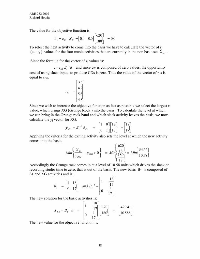
The value for the objective function is:
[ ]Π1 1 1 0 0 0 0620180
0 0= ′ =
=c XB B . . .
To select the next activity to come into the basis we have to calculate the vector of rj (cj - zj ) values for the four music activities that are currently in the non basic set XD1 . Since the formula for the vector of zj values is:
and since cdBcz B1
11−′= B1 is composed of zero values, the opportunity
cost of using slack inputs to produce CDs is zero. Thus the value of the vector of rj s is equal to cD1.
rj1
354 25 64 8
=
.
.
.
.Since we wish to increase the objective function as fast as possible we select the largest rj value, which brings XG (Grunge Rock ) into the basis. To calculate the level at which we can bring in the Grunge rock band and which slack activity leaves the basis, we now calculate the yj vector for XG.
y B dXG XG= =
=
−1
1 1 00 1
1817
1817
Applying the criteria for the exiting activity also sets the level at which the new activity comes into the basis.
MinXy
y Min MinBi
iXGiXG:
.
.>
=
=
0
6201818017
34 4410 58
Accordingly the Grunge rock comes in at a level of 10.58 units which drives the slack on recording studio time to zero, that is out of the basis. The new basis B2 is composed of S1 and XG activities and is:
B and B2 211 18
0 17
11817
01
17
=
=
−
−
The new solution for the basic activities is:
X B bB2 21
11817
01
17
620180
429 4110 588
= =−
=
−.
.
The new value for the objective function is:
38

ARE 252 2002 Richard Howitt
Π [ ]2 2 2 0 0 56429 4110 588
59 29= ′ =
=c XB . .
..
.
This level of return is clearly better than the initial solution of not using the resources at all, but is it the best use that we can make of the limited studio resources ?
With the new basis there is a new set of opportunity costs for the resources. Studio space is fully used on the Grunge band under the current allocation, but Airplay time still has a lot of slack. The new set of rj values are as follows:
[ ] [ ]51.141.045.01028
1432
1225
171017181
6.502
21
22222
−−=
−−′=
′−′=−= −
D
BDDD
c
DBcczcr
Using the maximum rj rule, the only music activity for which the marginal contribution to the objective function exceeds that of the Grunge band is XH ( Hiphop ). Therefore XH comes into the basis. The new yj values are:
y B dXH XH= =−
=
−2
11
1817
01
17
2810
17 4120 588
..
Applying the criteria for the exiting activity also sets the level at which the new activity comes into the basis.
MinXy
y Min MinBi
iXHiXH:
...
.
.
.>
=
=
0
429 4117 41210 580 588
24 6617 99
This says that the Grunge band should give up their studio time to the Hiphop band, and airplay time will still be slack. The next ( third ) basis has S1 and XH and is:
B and B3 311 28
0 101 2 80 01
=
=
−
−.
.The new solution for the basic activities is:
X B bB3 31 1 2 8
0 01620180
116 018 0
= =−
=
−.
...
The new value for the objective function is:
Π [ ]3 3 3 0 0 4 8116 018 0
86 4= ′ =
=c XB B . .
..
.
Clearly Hiphop is an improvement over the Grunge bands. The rj values for the new basis B3 are as follows:
39

ARE 252 2002 Richard Howitt
40
][ ] [r c z c c B D cD D D B D= − = ′ − ′ = ′ −−
= − − −−
3 3 3 3 31
3 3 0 4 81 2 80 01
2512
3214
1817
2 26 2 52 2 56..
.. . .
Since all the rj values for the third basis are negative this tells us that we are at the optimum solution with the Hiphop band using all the Studio time and Airplay time is in surplus. This problem is specified and solved in Gams over the page. Check the format of the Gams set up in matrix form. Note that every number on the Gams output has been, or can be, calculated in the matrix operations by hand. Remember that the “Duals” or “Marginals” on the resource constraints are calculated above in the rj equation as
. λ = ′ −c BB3 31
The Gams code to solve this problem and the resulting optimal solution for the problem can be downloaded from the Gams template part of the class webpage. Check that the matrix calculations agree relatively closely with the Gams printout.
ARE 252 2002 Richard Howitt
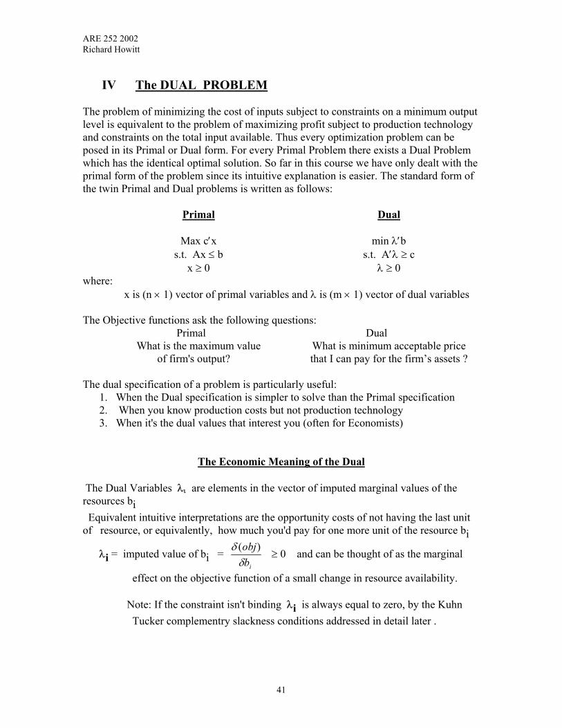
IV The DUAL PROBLEM The problem of minimizing the cost of inputs subject to constraints on a minimum output level is equivalent to the problem of maximizing profit subject to production technology and constraints on the total input available. Thus every optimization problem can be posed in its Primal or Dual form. For every Primal Problem there exists a Dual Problem which has the identical optimal solution. So far in this course we have only dealt with the primal form of the problem since its intuitive explanation is easier. The standard form of the twin Primal and Dual problems is written as follows: Primal Dual Max c′x min λ′b s.t. Ax ≤ b s.t. A′λ ≥ c x ≥ 0 λ ≥ 0 where: x is (n × 1) vector of primal variables and λ is (m × 1) vector of dual variables The Objective functions ask the following questions: Primal Dual What is the maximum value What is minimum acceptable price of firm's output? that I can pay for the firm’s assets ? The dual specification of a problem is particularly useful:
1. When the Dual specification is simpler to solve than the Primal specification 2. When you know production costs but not production technology 3. When it's the dual values that interest you (often for Economists)
The Economic Meaning of the Dual
The Dual Variables λι are elements in the vector of imputed marginal values of the resources bi Equivalent intuitive interpretations are the opportunity costs of not having the last unit of resource, or equivalently, how much you'd pay for one more unit of the resource bi
λi = imputed value of bi = δδ(objbi
) ≥ 0 and can be thought of as the marginal
effect on the objective function of a small change in resource availability.
Note: If the constraint isn't binding λi is always equal to zero, by the Kuhn Tucker complementry slackness conditions addressed in detail later .
41

ARE 252 2002 Richard Howitt
Dual Objective function The dual objective function λ′b is equal to the sum of the imputed values of the total resource stock of the firm. It is the sum of money that you would have to offer a firm owner to make them consent to a buy-out. Dual Constraints The dual constraints A′λ ≥ c can be interpreted as defining the set of prices λ for the fixed resources (or assets) ( b ) of the firm that would yield at least an equivalent return to the owner as producing a vector of products x, which can be sold for prices (c), from these resources. The dual constraint is a "greater than or equal to" because you can pay too much for a productive input, but market forces will ensure that you cannot count on buying an input for less than its value when turned into a saleable product.
Post multiplying the transpose of the technical input requirement matrix A by the dual prices λ results in an mx1 vector of marginal opportunity costs for each of the n potential production activities.
A′λ = vector of marginal opportunity costs of production.
For a single production activity xi its opportunity cost of production for a vector of dual prices λ is:
ai′λ = (column i of A)′ (λ vector)
ai′λ = (aij . . . ami)
λ
···
λm
= imputed cost of the last unit of xi produced, which equals the sum of imputed values of each resource needed times the amount of that resource needed to produce xi
↑ ↑
resource reqt.(coefficients)for input xi(one unit)
·
Marg. imputed
value (for 1 unit) of those resources
required
ai′λ = The cost of producing a unit of xi if I have to pay λ for resources b
42
ARE 252 2002 Richard Howitt
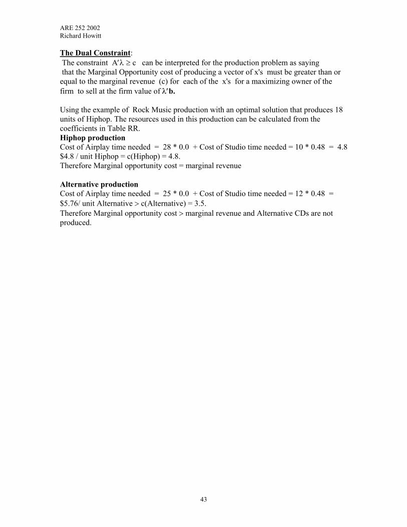
The Dual Constraint: The constraint A′λ ≥ c can be interpreted for the production problem as saying that the Marginal Opportunity cost of producing a vector of x's must be greater than or equal to the marginal revenue (c) for each of the x's for a maximizing owner of the firm to sell at the firm value of λ′b. Using the example of Rock Music production with an optimal solution that produces 18 units of Hiphop. The resources used in this production can be calculated from the coefficients in Table RR. Hiphop production Cost of Airplay time needed = 28 * 0.0 + Cost of Studio time needed = 10 * 0.48 = 4.8 $4.8 / unit Hiphop = c(Hiphop) = 4.8. Therefore Marginal opportunity cost = marginal revenue Alternative production Cost of Airplay time needed = 25 * 0.0 + Cost of Studio time needed = 12 * 0.48 = $5.76/ unit Alternative > c(Alternative) = 3.5. Therefore Marginal opportunity cost > marginal revenue and Alternative CDs are not produced.
43
ARE 252 2002 Richard Howitt
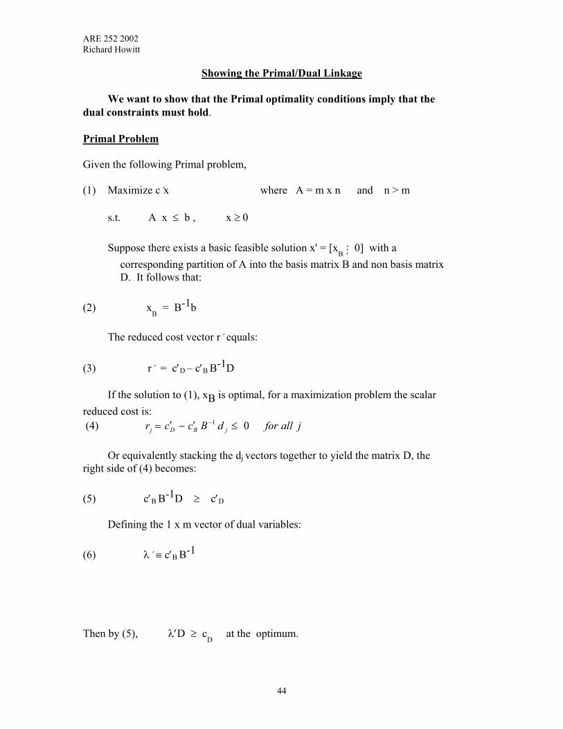
Showing the Primal/Dual Linkage
We want to show that the Primal optimality conditions imply that the dual constraints must hold. Primal Problem Given the following Primal problem, (1) Maximize c´x where A = m x n and n > m s.t. A x ≤ b , x ≥ 0 Suppose there exists a basic feasible solution x' = [x
B .: 0] with a
corresponding partition of A into the basis matrix B and non basis matrix D. It follows that:
(2) x
B = B-1b The reduced cost vector r´ equals: (3) r´ = c′D – c′B B-1D If the solution to (1), xB is optimal, for a maximization problem the scalar reduced cost is: (4) jallfordBccr jBDj 01 ≤′−′= −
Or equivalently stacking the dj vectors together to yield the matrix D, the right side of (4) becomes: (5) c′B B-1D ≥ c′D Defining the 1 x m vector of dual variables: (6) λ´ ≡ c′B B-1 Then by (5), λ′D ≥ c
D at the optimum.
44

ARE 252 2002 Richard Howitt
The shadow values of resources you'd need to bring xD's into basis ie (The opportunity costs of bringing activities into basis, times the input requirement )
≥
Marginal benefits of bringing xD's into the basis ( Since cjxj is the benefit from xj .cjxj = 0 when xj = 0 ,(that is xj is a non-basic activity)
Dual Problem The dual problem to (1) is specified as:
(7) 0≥≥′
′
λλλ
andcAtoSubjectbMinimize
We want to show that the dual solution vector λ defined in (6) is:
(a) Feasible - That is, it satisfies the constraints in (7), and
(b) Optimal - By showing that the dual objective function value is equal to the optimal primal objective function value.
(A) Feasibility of λ (8) λ´A = [λ´ B :: λ´ D] = [c′B B-1 B :: c′B B-1D]
= [c′B : c′B B-1D]
but substituting the inequality condition for optimality c in (5) we get: DB cDB ′≥′ −1
(9) [c′B : c′B B-1D] ≥ [ c′B : c′D] = c´ combining (8) and (9): (10) λ´A ≥ c´ transposing yields A´λ ≥ c Thus by definition λ is a feasible solution to the constraints A´λ ≥ c
45

ARE 252 2002 Richard Howitt
(B) Optimality of λ Using the dual objective function in (7) and our definition of λ in (6) we get: (11) λ´ b = c′B B-1 b = c′B x
B
↑
substitute the definition of xB = B-1b from (2)
∴ Dual Objective Function value = Optimal Primal Objective Function
value ∴ The dual value λ is optimal by the Strong Duality Theorem.* The Point: If the standard primal LP problem has an optimal basic
feasible solution with a basis B then the vector λ´ ≡ c′B B-1 is a feasible and optimal solution for the corresponding dual problem.
*Strong Duality Theorem: The theorem can be informally summarized as: λ´ b = c´x If and only if x and λ are optimal solutions to the primal and dual problems respectively
Numerical Matrix Example - Yolo Model
The A matrix in Yolo is 4 x 4 . The * denotes the basic solution activities and binding constraints for the optimal solution. * * Alfalfa Wheat Corn Tomato A = *Land 1.0 1.0 1.0 1.0 Water 4.5 2.5 3.5 3.25 Labor 6.0 4.2 5.6 14.0 *Contract 0.0 0.0 0.0 33.25 The optimal solution to Yolo has two binding constraints Land and Contract, and two non-zero activities Wheat and Tomatoes. We collapse the A matrix to the basis matrix B by removing the rows and columns that do not have * and do not constrain the optimal solution. That is, if the rows are not binding, their coefficients are not in the basis.
46
ARE 252 2002 Richard Howitt
The optimal basis matrix is therefore 2 x 2, ∴ ignoring the slack Labor and Labor constraints. The optimal basis B is:
B = D =
1 10 0
1 10 33.25
B-1 = b = 1 0.030070 0.03007
−
6006000
cB = 160825
(Note that for B to be invertible the number of activities in the basis must equal the number of binding constraints) Check the matrix derivations against the computer printout. (1) Optimal Primal Solution xB = B-1b (forget about xD; they are all zeroes)
xB = = = 1 0.030070 0.03007
−
6006000
(1)(600) ( 0.03007)(6000)(0)(600) (0.03007)(6000)
+ −+
419.58180.42
(2) Optimal Dual Solution (Marginals on Resources)
λ' = c'B B-1 = [ 160 , 825] 1 0.030070 0.03007
−
λ values in Gams are the "MARGINALS" on resources. (They are > 0 for binding constraints, = 0 for non-binding constraints)
= [(160)(1) + (825)(0) , (160)(-0.03007) + (825)(0.03007)] = [160 , 20] (3) rj = cj - zj z'j = c'
B B-1D = λ'D rj values in Gams are the "MARGINALS" on activities. (They = 0 on activities in basis,< 0 for non-basic activities )
z'j = [160 , 20]
1 10 0
= [160 , 160]
47

ARE 252 2002 Richard Howitt
cD = [121 , 135]
∴ r' = [121 , 135] - [160 , 160] = [ -39 , -25] (4) Optimal Objective Function Π = c'B x
B
Π = [160 825] = [67127.84 + 148872.07] = 216000 419.549180.451
Parametric Analysis Parametric analysis is the main method for obtaining policy results from optimization models. By changing the output prices or quantities of input available over a range of values we can generate empirical estimates of : (i) The Supply Function from the modeled process or (ii) The Derived Demand for inputs to the modeled process: We may also be concerned with the Sensitivity of the model. Sensitivity tests the stability of conclusions from the model when we change a constraint or coefficient value. This is useful when we are uncertain of the exact value of a parameter and need to know whether knowing the value precisely is important. Case: 1. Generating Derived Demand Functions for Inputs
The resource availability vector b is parameterized - that is, changed by small incremental values over a specified range. At each point the model is optimized and the value of the resource λ is plotted against the amount of the input b to form the derived demand function.
Given the Problem
Max c′x subject to. Ax ≤ b , x ≥ 0 The optimal solution is x = [x
B :: 0]
(Note: We assume the solution is not degenerate) ∴ x
B = B-1b
and ∆xB = B-1∆b
48
ARE 252 2002 Richard Howitt
Suppose ∆x
B is small enough so there is no change in the basis, then we can define
new x values, x which are defined as: x = [x
B + ∆x
B :: 0] These result in a new objective function value:
Objective Function: old Π = cB′x
B
new = cB′(x
B + ∆x
B) Π%
∆Π = Π% – Π = cB′∆x
B
= cB′B-1∆b
∆Π = λ ∆b Selecting the bith activity.
∴ ib∆
∆Π = λi Thus λ measures the impact on the objective function of a marginal
change in resource availability, given no change in the basis B. But from the equation for λ , ( λ′ = c
B′B-1 ) we see that for linear problems, the value of
λ does not change with ∆b unless (i) The basis B changes, or (ii) The objective function coefficients c
B are changed by parameterization.
Result
I. For LP problems, the marginal change in the objective function for changes in resources (∆Π/∆b) is constant until the basis changes.
II. When the basis changes, the value of λ changes due to new values in c
B′ and B.
This gives rise to the stepwise response to parameterization shown in the figure below.
49
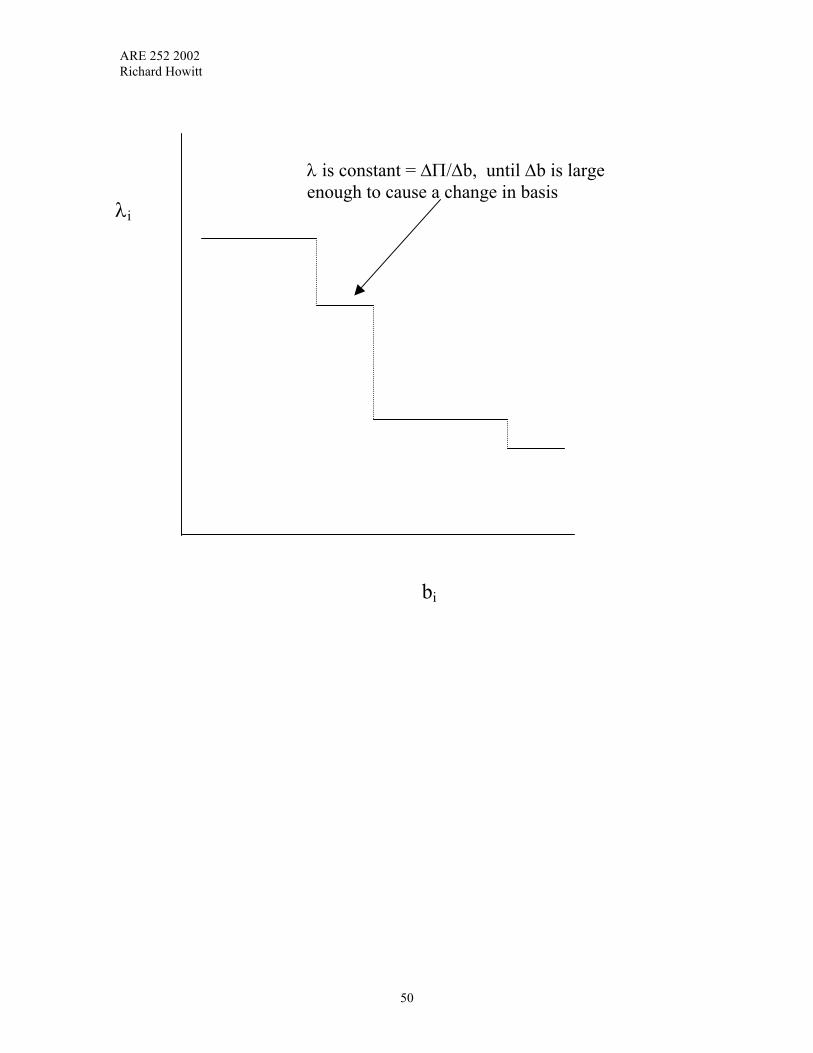
ARE 252 2002 Richard Howitt
λ is constant = ∆Π/∆b, until ∆b is large enough to cause a change in basis
λi
bi
50
ARE 252 2002 Richard Howitt
Case: 2. Generating Supply Functions for Outputs Similarly to the demand functions, supply functions are obtained by parameterizing a single objective function coefficient say, ci ,by small incremental values over a specified range. At each point the model is optimized and the quantity of the output xi produced is plotted against the “price” to form the supply function. Clearly, for LPs there will only be a change in the product xi when there is a change of basis caused by the change in ci. Accordingly, the reaction when xi is zero and therefore a non-basis activity is going to be different from the situation when xi > 0, and is in the basis. Case I Non-Basis activity supply parameterization If xi = 0 , then from the optimality conditions we know that the reduced cost for this activity ( assuming maximization) ri = ci – zi < 0 Since zi = λ′ di and λ′ = c′BB-1 the value of zi is unchanged by a change in ci because it is not in the vector cB. However, if the value of ci is increased by less than ri then the reduced cost will still be < 0 ( though reduced in numerical value) and xi will still be a non-basis variable. If ∆ci > ri , then ri will become positive and this will induce a change of basis which will bring the xi activity into the basis with a positive value. Case II Basis activity supply parameterization Consider parameterizing a basis variable xk. The coefficient ck is now part of the vector cB. Since xk is an optimal basic variable we know that rk = ck – zk = 0. Again, zk = λ′ dk and λ′ = c′BB-1 the value of zk is therefore changed by a change in ck and from the simplex criteria we know that:
(i) The basis will change since ∆ck will cause ∆λ, and some activities will leave the basis.
(ii) The new basis will have a larger value for xk since the reduced cost with the higher ck value in the basis value vector will increase the value of rk.
Thus whether we start with a non-basis or basic activity, parameterizing the objective coefficient over a discrete range will result in a series of stepped increases in the quantity of xk in the optimal solution. The resulting supply function will be an upward sloping supply function.
51
ARE 252 2002 Richard Howitt
Complementary Slackness Primal Complementary Slackness The concept of complementary slackness applies to both the primal and dual problems, but is easier to conceptually understand in the primal case. The formal proofs are developed for the dual CS case. Given the standard LP problem of:
Max c′x subject to. Ax ≤ b , x ≥ 0
The primal complementary slackness theorem says that for the jth constraint: If (bi - a′i x ) > 0 then λi = 0 Summarized as (bi - a′i x ) λi = 0 Or in summation form (bi - Σj aij xj ) λi = 0 In words this says that if the total use of the ith input in all productive uses is less than the amount of input available, then the marginal scarcity value of additional units of input is zero. Note there is a special case in which both (bi - Σj aij xj ) and λi are equal to zero. This says that the constraint is binding, but an additional unit of bi will not add to the objective function value. A corollary is: If λi > 0 then (bi - Σj aij xj ) = 0. That is to say, the shadow value cannot be positive if the constraint is not binding. To get an intuitive idea of the primal complementary slackness, imagine that you are sunbathing on a large, sandy, uncrowded and hot beach. If you are offered additional sand for $10 you are unlikely to purchase it, as your sand constraint is not binding. However if you are offered a cold drink ( you do not have any) you are probably willing to pay a substantial premium price over the supermarket price to get a cold drink on the beach.
52

ARE 252 2002 Richard Howitt
Dual Complementary Slackness The Standard Dual Problem is:
Min λ′b
s.t. A′λ ≥ c λ > 0 Theorem. Let x and λ be feasible solutions to the standard primal and dual problems. A necessary and sufficient condition for them to be optimal is: (i) If xi > 0 then λ'ai = ci Summarized by [ ] c' - λ'A x = 0 (ii) If λ'ai > ci then xi = 0. The “Free Lunch” Theorem Note xi is never < 0 by definition of feasibility, and ci is never > λ'ai by dual constraint that λ′Α ≥ c. The intuition for the direction of this constraint is that under economic (and optimizing ) assumptions λ′A < c cannot exist, as productive resources are never priced below their immediate productive value as this allows instantaneous capital gains. The possibility of such gains is ruled out by the "No Free Lunch" theorem. Proof Sufficiency (Sufficiency- If the conditions hold–then it is optimal.) Assume condition (i) or condition (ii) holds. Then: (1) [ ] c' - λ'A x = 0 ∴ λ'Ax = c'x Since Ax = b for any basic feasible solution ∴ λ'b = c'x ∴ by the Duality theorem λ and x must be optimal if λ'b = c'x Necessity (Necessity- If the problem is optimal–then the conditions hold). Assume optimality - if λ* and x* are optimal solutions then from (1) λ*′b = c′x* dropping the * notation ∴ λ′Ax = c ′x ∴ [ ] c' - λ'A x = 0
53
ARE 252 2002 Richard Howitt
Demonstrating Complementary Slackness Case 1. Show that if xi > 0 , then ci′ –λ'ai = 0 Verbally In the production problem "If something is produced in positive quantities (xi > 0) then its marginal revenue equals its marginal opportunity cost at the optimum" That is to say: (ci′ –λ'ai=0) We select the subset of x, x
B (The basis Partition of x), since only the xi's > 0 are in
the basis Given that the solution is optimal it implies that xi > 0 and all the ri values = 0 (The"rj" of each xi is the net benefit of bringing xi into the basis when xi is already in the basis) Writing the vector of ri 's for the basis vectors B, then ri = (c
B′ – c
B′ ) = 0 .
Rewriting this ri = c
B′ –c
B′ B-1B (Since rj= ( )Dcc BD
−1− Β′′ when xj is not in the basis)
∴ cB′–λ′B = 0 since ri = 0 for basis activities
∴ cB′ = λ′B (Note, the non-basis x
D are zero by definition ∴ c′–λ'A becomes c′–λ'B)
Case 2. Show that if xi = 0, then ci′ –λ'ai < 0 Verbally In the production problem "If a product is not produced at the optimum, its net revenue must be less than its opportunity cost" If x = 0 It implies that none of these x's are in basis. Therefore we have the set xD, the non-basis partition. ∴ c′ – λ′A becomes c
D′ – λ′D
Recall rj = cj – zj = ( )Dcc BD−1
− Β′′ = ( )DcD λ′′ − so the vector of rj's = c
D′–λ′D
Since all the rj's < 0 for non-basic xj's at optimal solution ∴ c
D′–λ′D < 0
∴ λ′D > cD′ or c′j - λ′dj < 0
Note the strict inequalities
54

ARE 252 2002Richard Howitt
55
Corollary
If λ and x are optimal dual and primal solutions it implies that [ ] c' - λ'A x = 0 for
all values.Example: Auto Dealer Hype "Trust me, this car is selling below my invoice cost."
If you believe this—drop the course.In this example, we are optimizing from the buyer’s perspective . The buyer wants
to minimize the price for a car with certain attributes. cj is the dealer's invoice cost, and
cars are traditionally sold as a vector of attributes and options on a base unit. Thus a"loaded" car will be composed of a base unit, air conditioning, FM stereo, "dealer's prep",etc. These attributes of the car are represented by the mx1 vector ai.
The dealer's problem is to assign a set of prices λ′ to the mx1 ai vector such that
λ′ ai - ci ≥ 0
Remember that prices on a car lot are always negotiable, and the buyer wants to minimizethe cost “out of the door” of a car with one of each of the mx1 set of attributes. That isto minimize λ'b. The dealer wants to convince you that at the price vector λ thecomplementry slackness theorem does not hold. The complementary slackness theoremsays that if the dealer truly has set prices λ below his invoice then:
λ′ ai - ci < 0
and the dealer will set xi = 0. That is the car which is priced below invoice is never in
stock when you get to the dealer since "It has just been sold."
Duality and Reduced Cost
Since λ is the vector of opportunity costs on the binding resources, and rj's form a vector
of revenue minus activity opportunity costs, they must be connected.
λ = cB′B-1
r = [cD′–c
B′B-1D]
= cD′–λ′D
Each individual element in the vector r, rj = cj – λd
where λ′dj = [λ1 . . . λm]
d1j···
dmj
Therefore λd is equal to the shadow value of inputs required to produce a unit of activityxj that is not currently in the basis.
ARE 252 2002 Richard Howitt
V CALIBRATING OPTIMIZATION MODELS Even with a constraint structure and parameters that are theoretically correct, it is highly unlikely that a model will calibrate closely to the base year data. This is inherent in the structure of models which are by definition simplified abstractions of the real systems. In the process of abstracting and simplifying a real system the model loses information and needs to be verified against actual behavior. Just as in econometric modeling there are two phases of model estimation and prediction, in optimization modeling there are the two phases of model calibration and simulation. Fundamentally, the calibration process is one of using a hypothesized function and data on input and output levels in the base year to derive specific model parameter values that "close" the model. By closing the model, we mean that the calibration parameters lead to the objective function being optimized for the base year conditions. Like econometrics, calibration methods assume that the observed actions are motivated by optimizing over some set of criteria. It follows that if we can derive the parameters, that when optimized, lead to the observed actions, we have derived the parameters most likely to have been used by the decison maker. Given that most optimization models are specified to optimize profits to economic decision makers, they can in theory be calibrated from the demand (price) or supply (cost) sides. Calibrating model prices by deriving demand parameters has been practiced by builders of large quadratic programming models for many years. However demand side calibration can only help when the model is on a large enough scale so that changes in output change product prices. In addition, because models are usually specified with several regions supplying a single market demand, using a small number of demand parameters cannot calibrate the cropping patterns over several regions. Calibrating on the Model Supply Side This section contains a short overview and critique of the traditional methods of calibrating the supply side of optimization models using linear constraints. The shortcomings of the constraint calibration methods lead to a discussion of ways to derive nonlinear supply functions that are based on observed behavior by decision makers, but calibrate the model in general. These methods are termed "Positive Mathematical Programming" (PMP) (Howitt 1995) since they are based on positive inferences from the base year data, rather than normative assumptions. A Review of Supply Side Constraint Calibration Programming models should calibrate against a base year or an average over several years. Policy analysis based on normative models that shows a wide divergence between base period model outcomes and actual production patterns is generally unacceptable. However, models that are tightly constrained can only produce the subset of normative results that the calibration constraints dictate. The policy conclusions are thus bounded by a set of constraints that are expedient for the base year but often inappropriate under policy changes. This problem is exacerbated when the model is built on a regional basis with very few empirical constraints but a wide diversity of crop production. For example, the Yolo model presented in the previous chapter is highly simplified with only four cropping activities, but still requires unrealistic constraints on the amount of labor that can be employed to produce all four crops in the optimal solution. While labor requirements do vary, they are subject to a labor supply. The supply function will increase labor available in a given quarter at an increased cost of overtime or operations
56
ARE 252 2002 Richard Howitt
performed by custom operators. To suggest that a more profitable crop in some policy scenario will never be grown beyond a certain limit because of labor constraints is to radically depart from the actual empirical solution. In addition to the labor constraint, the water constraint may also be artificially constraining if the farmers have access to groundwater or river pumping. More complex linear production models require more complicated constraint structure to reproduce the observed cropping pattern. In many traditional models the proportions of crops are restricted by "rotational" constraints or "flexibility" constraints. These constraints determine the optimal solution not only for the base year for which they are appropriate, but also for policy runs that attempt to predict the outcome of changed prices, costs or resource availability. The solution of the model under policy runs is therefore significantly restricted by the base year solution constraints. This section is a brief overview of some of the past calibration methods in mathematical programming models. For a more comprehensive discussion see Hazell and Norton (1986) or Bauer and Kasnakoglu (1990). It is worth noting that no single linear constraint calibration method has proved sufficiently satisfactory to dominate the mathematical programming literature. Previous researchers such as Day (1961) have attempted to provide added realism by imposing upper and lower bounds to production levels as constraints. McCarl (1982) advocated a decomposition methodology to reconcile sectoral equilibria and farm level plans. Both approaches require additional micro level data and result in calibration constraints influencing policy response. Meister, Chen, and Heady (1978), in their national quadratic programming model, specify 103 producing regions and aggregate the results to 10 market regions. Despite this structure, they note the problem of overspecialization and suggest the use of rotational constraints to curtail the overspecialization. However, it is comparatively rare that agronomic practices are fixed at the margin, more commonly they reflect net revenue maximizing trade-offs between yields, costs of production, and externalities between crops. In this latter case, the rotations are themselves a function of relative resource scarcity, output prices, and input costs. Hazell and Norton (1986) suggest six tests to validate a sectoral model. First, a capacity test checks whether the model constraint set allows the base year production. Second, a marginal cost test ensures that the marginal costs of production, including the implicit opportunity costs of fixed inputs, are equal to the output price. Third, compare the dual value on land with actual rental values. Three additional comparisons of input use, production level, and product price are also advocated. Hazell and Norton show that the percentage of absolute deviation for production and acreage over five sectoral models ranges from 7 percent to 14 percent deviation. The constraint structures needed for this validation are not defined. In contrast, the PMP approach ( Howitt 1995 ) achieves exact calibration in acreage, production and price. The PMP approach was applied to the Turkish Agricultural Sectoral Model (TASM) which is one of the models listed by Hazel and Norton. The resulting PMP version of TASM calibrated exactly with the base year (Bauer and Kasnakoglu 1988) and showed consistency in the parameters over the seven years used for calibration. A recent application of a PMP calibrated model ( U S Bureau of Reclamation, 1997) has been built to analyze the effects of large inter-sectoral water reallocations in California. The model termed the Central Valley Production Model (CVPM) was tested by out of sample predictions of regional crop acreage changes during a recent drought period. The CVPM . The predictions were close with three contract crops ( Sugar beet, Tomatoes, and Subtropical orchard)
57

ARE 252 2002 Richard Howitt
having a 14- 23 % error. The remaining nine crops had prediction errors below 7%. Regional crop acreage was predicted for eleven regions. For all of the regions the crop acreage predictions had errors below six percent. The calibration problem for farm level, regional, and sectoral LP models can be mathematically defined by the common situation in which the number of binding constraints in the optimal solution (m) are less than the number of non-zero activities ( n ) observed in the base solution. If the modeler is fortunate enough to have empirical data to specify, á priori, a constraint set that reproduces the optimal base year solution, then additional model calibration is clearly redundant. The PMP approach is developed for the majority of empirical model builders who, for lack of empirical justification, data availability, or cost, find that the empirical constraint set does not reproduce the base year result. The LP solution is an extreme point of the binding constraints. In contrast, the PMP approach views the optimal farm production as a boundary point which is a combination of binding constraints and first order conditions. Relevant constraints should be based on either economic logic or the technical environment under which the agricultural production is operating. Calibration problems are especially prevalent where the constraints represent allocatable inputs, actual rotational limits and policy constraints. When the basis matrix has a rank less than the number of observed base year activities, the resulting optimal solution will suffer from overspecialization bias of production activities compared to the base year. A root cause of these problems is that linear programming was originally used as a normative farm planning method where full knowledge of the production technology is assumed. Under these conditions, any production technology can be represented as a linear Leontief specification, subject to resource and stepwise constraints. For aggregate policy models, this normative approach over simplifies the production and cost technology due to inadequate knowledge. In most cases, the only regional production data is an average or "representative" figure for crop yields and inputs. This common data situation means that the analyst using linear production technology in programming models is attempting to estimate marginal behavioral reactions to policy changes, based on average data observations. The average conditions can be assumed to be equal to the marginal conditions only where the policy range is small enough to admit linear technology over the whole range. Two broad approaches have been used to reduce the specialization errors in optimizing models. The demand-based methods have used a range of methods to add risk or endogenize prices. These have reduced the calibration, problem but substantial calibration problems remain in many models, Just (1993). A common alternative approach is to constrain the crop supply activities by rotational (or flexibility) constraints or step functions over multiple activities (Meister, Chen, and Heady, 1978). In regional and sectoral models of farm production, the number of empirically justifiable constraints are comparatively few. Land area and soil type are clearly constraints, as is water in some irrigated regions. Crop contracts and quotas, breeding stock, and perennial crops are others. However, it is rare that some other traditional programming constraints such as labor, machinery, or crop rotations are truly restricting to short-run marginal production decisions. These inputs are limiting, but only in the sense that once the normal availability is exceeded, the cost per unit output increases due to overtime, increased probability of machinery failure or disease. In this situation the analyst has a choice. If the assumption of linear production (cost) technology is retained, the observed output levels infer that additional binding
58

ARE 252 2002 Richard Howitt
constraints on the optimal solution should be specified. Comprehensive rotational constraints are a common example of this approach. An alternative explanation of the situation where there are more crop activities than constraints is that the profit function is nonlinear in land for most crops, and the observed crop allocations are a result of a mix of unconstrained and constrained optima. The equilibrium conditions for this case would be satisfied if some of all of the cropping activities had decreasing returns to land as acreage was increased. The most common reasons for a decreasing gross margin per acre are declining yields due to heterogeneous land quality, risk aversion, or increasing costs due to restricted management or machinery capacity. Positive Mathematical Programming
The positive mathematical programming (PMP) approach is being adopted quite rapidly for agricultural sector models. In their introduction to their book on “Agricultural Sector Modelling and Policy Information Systems”(2001) Heckelei et al state that they received
“a rich supply of about 60 proposals from 16 countries reflecting the breadth of work directed to agricultural sector modeling and policy information systems. Because the sample of proposals is indicative of current emphasis in research, it is worth mentioning that, from a methodological point of view almost 25% of the supply might be called “econometric partial’ analyses, another 25% “programming models” (half of which relying on PMP) whereas the remaining half of the proposals covered a multitude of quantitative methods..” Behavioral Calibration Theory The process of calibrating models to observed outcomes is an integral part of constructing physical and engineering models but is rarely formally analyzed for optimization models in agricultural economics. In this section we show that observed behavioral reactions yield a basis for calibrating models in a formal manner that is consistent with microeconomic theory. Analogously to econometrics, the calibration approach draws a distinction between the two modeling phases of calibration (estimation) and policy prediction. On a regional level, the information on the product output levels and farm land allocations is usually more accurate than the estimates of marginal crop production costs. This is particularly true when micro data on land class variability, technology, and risk feature in the farmers' decisions, but are absent in the aggregate cost data available to the model builder. Accordingly, the PMP approach uses the observed acreage allocations and outputs to infer marginal cost conditions for each regional crop allocation observed. This inference is based on parameters that are known to be accurately observed and the usual profit maximizing and concavity assumptions. The Nonlinear Calibration Proposition states: If the model does not calibrate to observed production activities with the full set of general linear constraints that can be empirically justified. A necessary condition for profit maximization at the observed values is that the objective function is nonlinear in at least some of the activities.
59
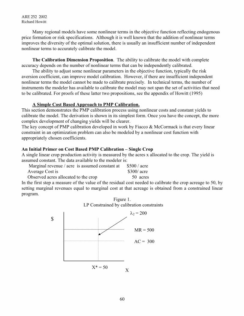
ARE 252 2002 Richard Howitt
Many regional models have some nonlinear terms in the objective function reflecting endogenous price formation or risk specifications. Although it is well known that the addition of nonlinear terms improves the diversity of the optimal solution, there is usually an insufficient number of independent nonlinear terms to accurately calibrate the model. The Calibration Dimension Proposition. The ability to calibrate the model with complete accuracy depends on the number of nonlinear terms that can be independently calibrated. The ability to adjust some nonlinear parameters in the objective function, typically the risk aversion coefficient, can improve model calibration. However, if there are insufficient independent nonlinear terms the model cannot be made to calibrate precisely. In technical terms, the number of instruments the modeler has available to calibrate the model may not span the set of activities that need to be calibrated. For proofs of these latter two propositions, see the appendix of Howitt (1995) A Simple Cost Based Approach to PMP Calibration. This section demonstrates the PMP calibration process using nonlinear costs and constant yields to calibrate the model. The derivation is shown in its simplest form. Once you have the concept, the more complex development of changing yields will be clearer. The key concept of PMP calibration developed in work by Fiacco & McCormack is that every linear constraint in an optimization problem can also be modeled by a nonlinear cost function with appropriately chosen coefficients.
An Initial Primer on Cost Based PMP Calibration – Single Crop A single linear crop production activity is measured by the acres x allocated to the crop. The yield is assumed constant. The data available to the modeler is: Marginal revenue / acre is assumed constant at $500 / acre Average Cost is $300/ acre Observed acres allocated to the crop 50 acres In the first step a measure of the value of the residual cost needed to calibrate the crop acreage to 50, by setting marginal revenues equal to marginal cost at that acreage is obtained from a constrained linear program.
Figure 1. LP Constrained by calibration constraints
MR = 500
λ2 = 200 $
AC = 300
X* = 50 X
60

ARE 252 2002 Richard Howitt
1. From the nonlinear calibration proposition we know that either (or both) the cost or production function is nonlinear if we need calibration constraints. In this case we define the total cost function to be quadratic in acres (x) .There are very many possible nonlinear forms, but this is the simplest general form. TC = α x + ½ γ x2
2. Under optimization, if unconstrained, crop acreage expands until the marginal cost equals marginal revenue. Therefore MC = MR at x = 50
3. It follows that the value λ2 in the linear model is the difference at the constrained calibration value
and is equal to MR - AC . But from step 2 we know that MR = MC therefore λ2 = MC – AC, since MR = MC at x = 50 Given the hypothesized total cost function TC :
MC = α + γ x AC = α + ½ γ x therefore MC - AC = α + γ x - (α + ½ γ x )
Therefore λ2 = MC - AC = ½ γ x and the cost slope coefficient is calculated as: γ = 2λ/ x* = (2 * 200)/ 50 = 8
4. We can now calculate the value of α using the AC information in the basic data set as: 300 = α + ½ * 8 * 50 Therefore α = 300 - 200 = 100
5. Using the values for α and γ the unconstrained quadratic cost problem is: Max Π = 500 x - α x - ½ γ x2 = 500 x - 100 x - ½ 8 x2
δΠ / δx = 500 - 100 - 8 x
Solving for δΠ / δx = 0 which implies MR = MC
8 x = 400 therefore x* = 50.
NOTE that the unconstrained model calibrates exactly in x and also in Π
Also note that: (a) MC = MR at x= 50 (b) AC = 300 at x= 50
(c) The cost function has been “tilted” (d) Two types of information are used x* and AC
61

ARE 252 2002 Richard Howitt
(e) The observed x* quantities need to mapped into value space by the LP before it
can be used
(f) The model now reflects the preferences of the decision maker (g) The model is unconstrained by calibration constraints for policy analysis An Analytic Derivation of Calibration Functions
This section will show that the PMP non-linear calibration approach can be applied to any non-degenerate linear problem. The derivation of the general result proceeds in three steps. The first step shows that the dual value on the calibration constraint for the calibrated activity set xk is equal to the reduced cost of the activity xi in the un-calibrated base problem. The second step shows that if the correct non-linear penalty function is added to the objective function, the resulting nonlinear problem satisfies the necessary conditions for optimality at the required value of xi. Finally, it is shown that the correct penalty function has a gradient at the required value of xi equal to the negative of the calibration dual
The general linear programming optimization problem can be compactly written as:
(1) 0≥
≤
′
xbAxtoSubject
xcMaxx
Where c is an p x 1vector of net returns per unit activity, and the matrix A and right hand side b are the usual technical constraints and right hand sides. The dimension of A is m x p, (m < p). The basis dimension of A is m. If the number of observed activities is n (n ≤ p), where n = k + m, then in addition to the xm basis activities, there are an additional k activities xk that are observed and need to be calibrated into the optimal model solution. For simplicity, define the LP problem as only subject to one set of upper bound calibration constraints:
(2)
0
~
≥+≤
≤
′
xxxI
bAxtoSubjectxcMaxx
ε
where the ε is added to the calibration constraints to prevent degeneracy.
The optimal basic solution to this problem will have a mix of n binding resource and calibration constraints. The A matrix can be partitioned into an m x m basis matrix B that corresponds to the m least profitable "marginal" activities ( xm ) , and an associated m x k matrix N for the k calibrated
62
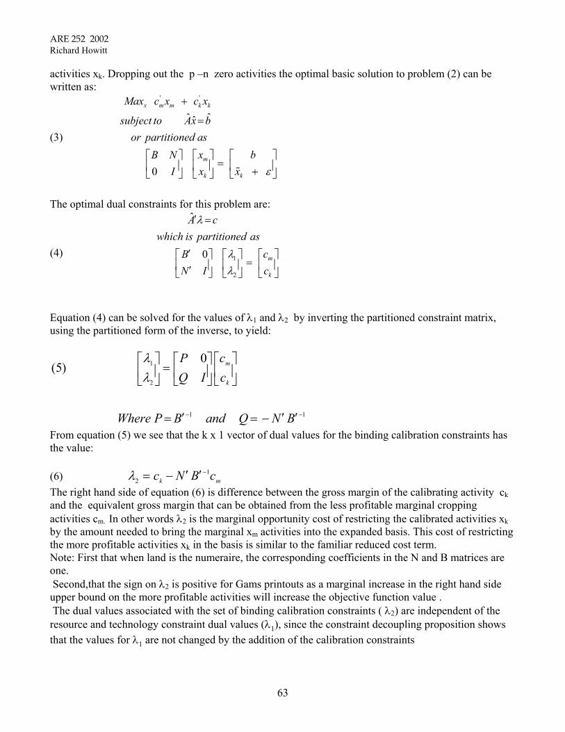
ARE 252 2002 Richard Howitt
activities xk. Dropping out the p –n zero activities the optimal basic solution to problem (2) can be written as:
(3)
' '
ˆˆ ˆ
0
x m m k k
m
k k
Max c x c x
subject to Ax bor partitioned as
x bB Nx xI ε
+
=
= + %
The optimal dual constraints for this problem are:
(4) 1
2
ˆ
0 m
k
A cwhich is partitioned as
cBcN I
λ
λλ
′ =
′ = ′
Equation (4) can be solved for the values of λ1 and λ2 by inverting the partitioned constraint matrix, using the partitioned form of the inverse, to yield:
11
2
1 0)5(
−− ′′−=′=
=
BNQandBPWhere
cc
IQP
k
m
λλ
From equation (5) we see that the k x 1 vector of dual values for the binding calibration constraints has the value:
(6) mk cBNc 1
2−′′−=λ
The right hand side of equation (6) is difference between the gross margin of the calibrating activity ck and the equivalent gross margin that can be obtained from the less profitable marginal cropping activities cm. In other words λ2 is the marginal opportunity cost of restricting the calibrated activities xk by the amount needed to bring the marginal xm activities into the expanded basis. This cost of restricting the more profitable activities xk in the basis is similar to the familiar reduced cost term. Note: First that when land is the numeraire, the corresponding coefficients in the N and B matrices are one. Second,that the sign on λ2 is positive for Gams printouts as a marginal increase in the right hand side upper bound on the more profitable activities will increase the objective function value . The dual values associated with the set of binding calibration constraints ( λ2) are independent of the resource and technology constraint dual values (λ1), since the constraint decoupling proposition shows that the values for λ1 are not changed by the addition of the calibration constraints
63

ARE 252 2002 Richard Howitt
If an increasing nonlinear cost function is added to the objective function for the xK activities that need to be calibrated the marginal and average costs of producing xK will differ. The net return to land from xK now decreases as the acreage is increased. The net returns to land from xK reach an internal equilibrium solution at the point where they are equal to the opportunity cost of land set by the marginal crops xM. If the calibration constraints are removed and a nonlinear cost for xK is added, problem (2) becomes:
(7) [ ] bxx
NBtoSubject
xfxcxcMax
k
m
kkkmmx
=
−+ )(''
The reduced gradient ( the nonlinear equivalent of the reduced cost) for activities xk is derived by rewriting the set of binding constraints in (7) so that xm is a function of xk : (8) km xNBbBx 11 −− −=
Substituting the expression for xm back into the objective function in (7) defines the problem as an unconstrained function of xk . (9) )()( 11
kkkkm xfxcxNBbBcMax −′+−′ −−
The unconstrained gradient of this nonlinear problem in xk is defined as the reduced gradient and is:
(10) )()(
)(1
kk
kmk
xfofgradienttheisxfwherexfcBNc
∇
′∇−′′− −
Luenberger ( 1984) shows that a zero valued reduced gradient is a necessary condition for the optimum of a nonlinear problem. The calibrated problem (7) will optimize with a zero reduced gradient at the values kx% when or substituting into equation (6), when )(1
kmk xfcBNc ′∇=′′− −2)( λ=′∇ kxf .
Proposition: If the parameters of f(x) are calibrated such that at the value kx% , 2)~( λ=′ kxf∇ the model will be optimal exactly at the calibrating acres. To reiterate, equation (6) shows that λ2 is equal to the first two terms of equation (10). It follows that the reduced gradient of the resulting nonlinear problem will equal zero at Kx~ . As this is a necessary condition for the optimum, the problem in equation (7) will calibrate at the values x~ without calibration constraints.
64

ARE 252 2002 Richard Howitt
Equation (9) shows that optimal solution to the calibrated problem responds to changes in the linear
gross margin “c” , the right hand side values “b”, or the constraint coefficients “B or N ”. The economic interpretation of the calibration cost function f(xK) is as follows. From equation (6)
we see that λ2 is equal to the difference between the gross margins per unit land for xK and xM. The gross margins are calculated from the observed average variable costs. It follows that:
(11) λ2 = ( PK YK - ACK) - ( PM YM - ACM) but since the gross margin for the marginal crop xM is equal to the opportunity cost of land, and
since the land coeffcients in N and B equal one, using equations (5) and (6) we can rewrite (11) as: (12) λ2 = ( PK YK - ACK) - λ1 or λ2 + λ1 = ( PK YK - ACK) but by the equimarginal principle, at the optimal allocation of land, all crops must have a marginal
net return equal to the opportunity cost of land, therefore at the optimal solution to the nonlinear problem defined by equation (7):
(13) λ1 = PK YK - MCK = PK YK - ACK - ( MCK - ACK) substituting (12) into (13) yields: (14) λ2 = MCK - ACK
To summarize, this section has shown that linear and nonlinear optimization problems can be exactly calibrated by the addition of a specific number of nonlinear terms. We have used a general nonlinear specification to show that since the calibrated problem (2) yields the necessary conditons (6). If the nonlinear problem (7) has a nonlinear cost function f(xK) that satisfies equations (6), (10), and (14), the resulting nonlinear problem will calibrate exactly in the primal and dual values of the original problem, but without any inequality calibration constraints. In the next section we show how the calibration procedure can be simply implemented using a quadratic cost function in a two-stage process that is initiated with a calibrated linear program. An Empirical Calibration Method The previous section showed that if the correct nonlinear parameters are calculated for the (k- m) unconstrained (independent) activities, the model will exactly calibrate to the base year values x without additional constraints. The problem addressed in this section is to show how the calibrating parameters can be simply and automatically calculated using the minimal data set for a base year LP. Given that nonlinear terms in the supply side of the profit function are needed to calibrate a production model, the task is to define the simplest specification that is consistent with the technological basis of agriculture, microeconomic theory and the data base available to the modeler.
65

ARE 252 2002 Richard Howitt
A highly probable source of nonlinearity in the profit function is due to heterogeneous land quality. This will cause the marginal cost per unit of output to increase as the proportion of a crop in a specific area is increased. This phenomenon, first formalized by Ricardo (Peach (1993)), is widely noted by farmers, agronomists, and soil scientists, but often omitted from quantitative production models. Defining yields per acre as constant and marginal cost as increasing in land allocation is a considerable simplification of the complete production process. Given the applied goal of this "positive" modeling method, the calibration criteria used is not whether the simple production specification is true, but rather, does it capture the essential behavioral response of farmers, and can it be made to work with the restricted data bases and model structures available. The output qi from a given cropping activity "i" under a Leontieff production specification with land xi and two other inputs is :
(15) qi = Min (xi, ai2xi, ai3xi) yi In many LP problems such as the Yolo example, the objective function coefficients ci represent the Gross margin per acre faced by the farmer. The ci coefficient is composed of the product of the average yield, the price per unit output, with the average variable costs deducted. Since we are specifying the yield as constant but the marginal cost as increasing with acreage in this model, we have to separate these components. The calibrated optimization problem equivalent to equation (7) with land as the restricting factor becomes
(16) Max Σi Pi Yi xi – (αi + 0.5 γi xi )xi - ωj aij xi 3
2=j∑
subject to A x ≤ b and x ≥ 0 where ai1 = 1 and A = (mxn) with elements aij , xi is the acreage of land allocated to crop i, Yi is the yield per acre, αi and γi are respectively the intercept and slope of the marginal cost function per acre, and ωj is the cost per unit of the jth input. The PMP calibration approach uses three stages. In the first stage a constrained LP model is used to the dual values for both the resource and calibration constraints, λ1 and λ2 respectively. In the second stage, the calibrating constraint dual values (λ2 ) are used, along with the data based average yield function, to uniquely derive the calibrating cost function parameters (αi and γi). In the third stage, the cost parameters are used with the base year data to specify the PMP model in equation (16). The resulting model calibrates exactly to the base year solution and original constraint structure. The procedure is illustrated using a very simple problem which has a single land constraint (5 acres) and two crops wheat and oats. The following parameters are used:
Wheat (w) (Oats) (o)
66

ARE 252 2002 Richard Howitt
Crop prices Pw = $2.98/bu. Po = $2.20/bu.
Variable cost/acre ωw = $129.62 ωo = $109.98 Average yield/acre y– w = 69 bu. y– o = 65.9 bu.
The observed acreage allocation in the base year is 3 acres of wheat and 2 acres of oats. Figure 2 shows the initial problem in a diagrammatic form for two activities, with one resource constraint and two upper bound calibration constraints. Note that at the optimum, the calibration constraint will be binding for wheat, the activity with the higher average gross margin, while the resource constraint will restrict the acreage of oats.
Figure 2.
3+ε
ωW
o oP y
W WP y
λ1
67
λ1
λ2
2+ε
0 Acres Oats Acres WheatωO

ARE 252 2002 Richard Howitt
The problem in Figure 2 is: (17) Max (2.98*69 – 130) xw + (2.20*65.9 – 110) xo subject to (i) xw + xo ≤ 5 (ii) xw ≤ 3.01 (iii) xo ≤ 2.01 Note the addition of the ε perturbation term (0.01) on the right hand side of the calibration constraints. The average gross margin from wheat is $76/acre and oats $35/acre. The optimal solution to the stage 1 problem is when the wheat calibration constraint is binding at a value of 3.01 and constraint (i) is binding when the oat acreage equals 1.99. The oat calibration constraint is slack. Two equations are solved for the two unknown yield parameters (α and γ). Using the quadratic total land cost function specified in (16) and the first order conditions in equation (10), the first equation for the marginal cost coefficient sets λ2 equal to the difference between marginal and average cost based on equation(14) and derives the calibrated value for γ .
'2
2
2
( )(18) 0.5
2
k k
k k k
kk
k
f xx
x
λγ λ
λγ
∇ ==
=
%
%
%
Equation ( 18) uses the value of the dual on the LP calibration constraint (λ2) which is shown in figure 1 to be the difference between the average cost (AC) of the crop and the marginal cost (MC). The second equation is the average cost for crop i, y– i:
(19) Σij ωi aij = ci = αi + 0.5 γi xi ∴ αi = ci – 0.5 γi xi The derivation of the two types of dual value λ1 and λ2, can be shown for the general case (Howitt 1995). The A matrix in ( 2 ) is partitioned by the optimal solution into an m×m matrix B associated with the marginal variables xm , an m×1 subset of x with inactive calibration constraints. The second partition of A is into an m×k matrix N associated with a k×1 partition of x, xN of non-zero activities constrained by the calibration constraints. The equation for λ1 is the usual LP form of : (20) λ1 = B–1 mc′
68

ARE 252 2002 Richard Howitt
The elements of vector xm are the acreages produced in the crop group limited by the general constraints, and λ1 are the dual values associated with the set of m×1 binding general constraints. Equation (20) states that the value of marginal product of the constraining resources is a function of the revenues from the constrained crops. The “independent” crops (xk) do not influence the dual value of the resource by the decoupling proposition. This is consistent with the principle of opportunity cost in which the marginal net return from a unit increase in the constrained resource determines its opportunity cost. Since generally the more profitable crops xk are constrained by the calibration constraints, the less profitable crop group xm are those that could use the increased resources and hence set the opportunity cost. Equation (21) determines the dual values on the upper bound calibration constraints on the crops. (21) λ2 = – N' B'–1 cm + I ck and substituting (20) = I ck – N' λ1 The dual values for the binding calibration constraints are equal to the difference between the marginal revenues for the calibrated crops (xk) and the marginal opportunity cost of resources used in production of the constrained marginal crops (xm). Since the stage I problem in Figure 2 has a linear objective function, the first term in (21) is the crop average value product of land in activities xk. The second term in (21) is the marginal opportunity cost of land from equation (20). In this PMP specification, the difference between the average and marginal cost of land is attributed to changing land quality. Thus the PMP dual value (λ2) is a hedonic measure of the difference between the average and marginal cost of land, for the calibrated crops. Analogously to revealed preference, PMP can be thought of as revealed efficiency based on observed land allocations. Equation (21) substantiates the dual values shown in Figure 2, where the duals for the calibration constraint set (λ2) in the stage I problem are equal to the divergence between the LP average cost per acre and the marginal opportunity cost per acre. The dual value on land (λ1) is $35 and on the two calibration constraints (λ2) = [41 and 0]. Using equation (14), the λ2 value for wheat and the base year data, the cost function slope for wheat is calculated as: (22) γw = 2* 41/ 3 = 27.333 γw is now substituted into equation (19) to calculate the cost intercept αw. (23) αw = 129.62 - (0.5 * 27.333 * 3) = 88.62.
69

ARE 252 2002 Richard Howitt
Using the yield function parameters, the Stage II primal PMP problem becomes: (see Figure 3). (24) Max (2.98*69)xw + (2.20*65.9) xo - (88.62 + 0.5*27.333 xw) xw – 109.98 xO
subject to xw + xO ≤ 5
Figure 3.
3+ε
λ1 γW xW
A quick empirical check of the calibration to the base values is performed by calculating thacre of wheat at 300 acres. If it is close to the VMP (VAP) of oats and converging, the mocalibrate without the additional calibration constraints. The marginal cost per acre of wheat is:
MCw=3 = 88.62 + 27.333 * 3 = 170.619
VMPw=3 = 2.98* 69 – 170.619 = 205.62 –170.619 = 35.001
VMPO = 2.20* 65.9 – 110 = 144.98 – 110 = 34.98
The VMP for wheat at 3 acres of $35.01 is marginally above the VMP for oats ($34.98). Tunconstrained PMP model will calibrate within the rounding error of this example. _________________________________________________________________________
A Lagrangian Approach to PMP - the Wheat / Oats Farm Example
70
λ1
2+ε
0 Acres Oats Acres WheatαW
e VMP per del will
hus, the
__________
ARE 252 2002 Richard Howitt
The farm example on page 64 can be further simplified and made consistent with the analytical derivation by only considering the gross margins. GM Wheat = $76, GM Oats = $35. The LP problem is: Max 76 Xw + 35 Xo subject to Xw + Xo ≤ 5 Xw ≤ 3 + ε
Xo ≤ 2 + ε When we run this problem we will get Xw = 3 + ε, and X2 = 2 - ε. The land constraint will be binding with a shadow value of λ1 = 35. The other binding constraint will be the first calibration constraint with a shadow value λ2 of (76 - 35 ) = 41.
Define a PMP cost function f(X) = 0.5 γ X2 . f ' (X) = γ X
From the PMP theory λ2 = f ' (X) = γ X = 41 when X = 3.
therefore γ = 41/3 = 13.666.
The new PMP problem is: Max 76 Xw + 35 Xo - 0.5 ( 13.66 ) X2w
subject to Xw + Xo ≤ 5
The Lagrangian for this problem is: L = 76 Xw + 35 Xo - 0.5 (13.66 ) X2
w + φ ( 5 - Xw - Xo )
The first order conditions are:
76 13.666 0
35 0
5 0
ww
o
w o
L XXLXL X X
δ φδδ φδδδφ
= − −
= − =
= − − =
=
Solving the second FOC, yields φ = 35. Substituting this into the first FOC results in 76 - 13.666 Xw - 35 = 0 Therefore Xw = 41/ 13.666 = 3.0.
Substituting this into the third FOC yields 5 - 3 - Xo = 0 , Xo = 2.
NOTE. The PMP problem calibrates at exactly the required crop production acres. _____________________________________________________________________________
71
ARE 252 2002 Richard Howitt
This numerical example shows that PMP models can be calibrated using simple methods. The three stage process and calculation of the parameters is easily programmable as a single process using GAMS/MINOS. Thus, given the initial data and specifications, the PMP model is automatically calibrated in the time it takes to solve an LP and QP solution for the model. The basic PMP model specified in (24) calibrates in all aspects. That is, the optimal solution, binding constraints, objective function value and dual values will all be within rounding error of the original LP in (16) that is constrained by the calibration constraints. Despite all the notation, the basic concept of PMP is numerically simple and easy to solve automatically on desktop computers. An alternative calibration approach assumes that the cost per acre is constant , but the yield per acre declines with increased acres to any given crop. It can be shown that this assumption has the equivalent effect on the profit function as increasing costs. Both specifications can be justified from an agronomic point of view. The cost calibration approach is more common than the yield method. The original PMP article ( Howitt 1995) uses a yield based calibration method due to intransigent reviewers. The Gams code for the Yolo model without the artificial labor and water constraints, but calibrated using PMP is found in chapter 11. Calibration Using Elasticity Estimates Since the PMP procedure solves for the marginal cost function it also solves for the range of supply elasticities based on the marginal costs. However, as can be seen from equation (18), the marginal cost parameter γK depends on the empirical parameters of λ2 and Kx% . The resulting supply elasticity is not bounded and thus can assume values for a one period calibration that may be inconsistent with estimates based on a larger representative sample of crop response. The elasticity of supply is the essential measure of how the calibrated PMP model responds to policy changes. Accordingly, and consistent with the philosophy of using the best information available, the modeler must check the equilibrium elasticities implied by the calibrated cost functions, and if reliable parameters are available, use the prior information on elasticities to calibrate the model. The PMP marginal cost slope is calibrated against prior econometric estimates, but also reflects the conditions that are present in the base year model conditions. Modelers should be aware that using an elasticity based on prior econometric estimates to calculate the adjustment value does not ensure a positive net return. Net returns over variable costs should be checked after the adjustment factor is calculated. The supply elasticity based on prior econometric estimates is defined as:
QP
pq
s δδη =
Using the assumption of a constant per acre yield and the usual marginal cost supply function specification, the elasticity can be rewritten in terms of crop land allocations as:
*(25) sx Pc x
δηδ
= or *
s x xP c
η δδ
=
72
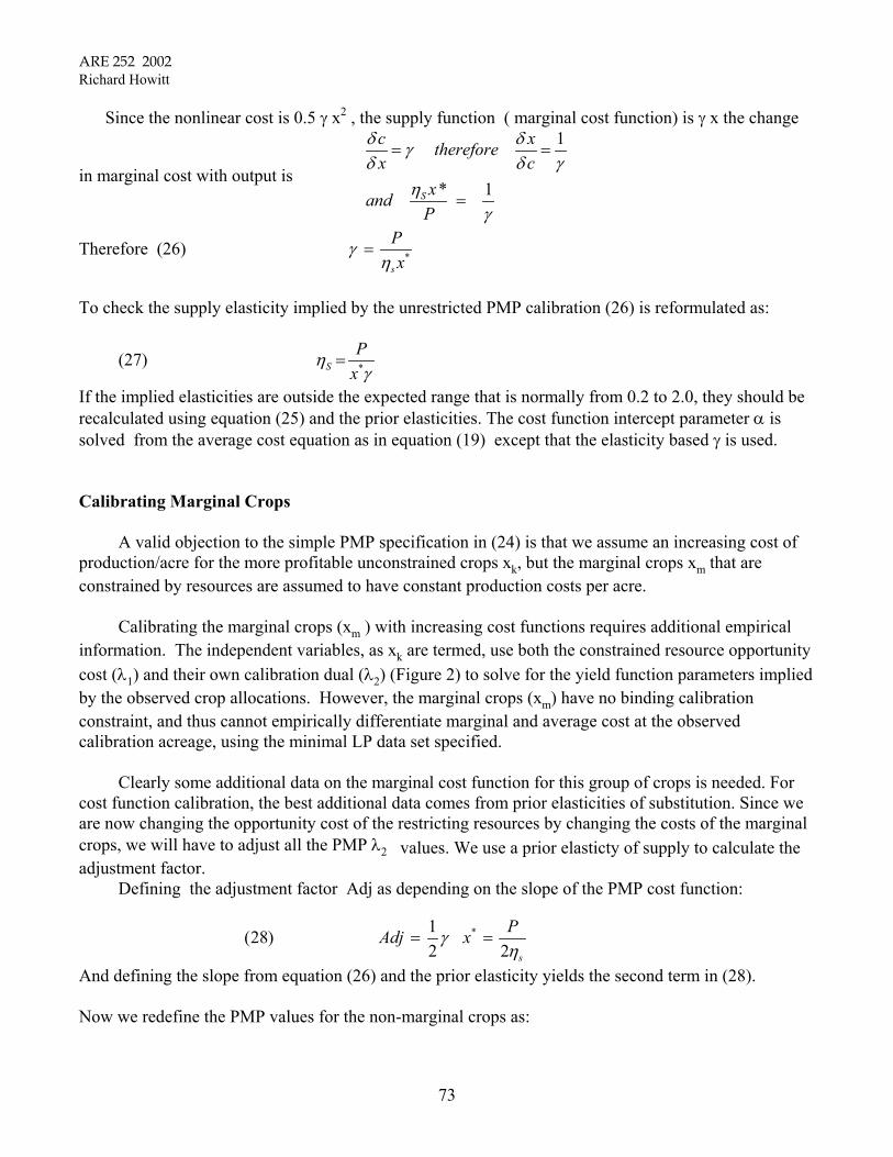
ARE 252 2002 Richard Howitt
Since the nonlinear cost is 0.5 γ x2 , the supply function ( marginal cost function) is γ x the change
in marginal cost with output is
1
* 1S
c xthereforex c
xandP
δ δγδ δ γ
ηγ
= =
=
Therefore (26) *s
Px
γη
=
To check the supply elasticity implied by the unrestricted PMP calibration (26) is reformulated as:
(27) *SP
xη
γ=
If the implied elasticities are outside the expected range that is normally from 0.2 to 2.0, they should be recalculated using equation (25) and the prior elasticities. The cost function intercept parameter α is solved from the average cost equation as in equation (19) except that the elasticity based γ is used. Calibrating Marginal Crops A valid objection to the simple PMP specification in (24) is that we assume an increasing cost of production/acre for the more profitable unconstrained crops xk, but the marginal crops xm that are constrained by resources are assumed to have constant production costs per acre. Calibrating the marginal crops (xm ) with increasing cost functions requires additional empirical information. The independent variables, as xk are termed, use both the constrained resource opportunity cost (λ1) and their own calibration dual (λ2) (Figure 2) to solve for the yield function parameters implied by the observed crop allocations. However, the marginal crops (xm) have no binding calibration constraint, and thus cannot empirically differentiate marginal and average cost at the observed calibration acreage, using the minimal LP data set specified. Clearly some additional data on the marginal cost function for this group of crops is needed. For cost function calibration, the best additional data comes from prior elasticities of substitution. Since we are now changing the opportunity cost of the restricting resources by changing the costs of the marginal crops, we will have to adjust all the PMP λ2 values. We use a prior elasticty of supply to calculate the adjustment factor. Defining the adjustment factor Adj as depending on the slope of the PMP cost function:
*1(28)2 2 s
PAdj xγη
= =
And defining the slope from equation (26) and the prior elasticity yields the second term in (28).
Now we redefine the PMP values for the non-marginal crops as:
73
ARE 252 2002 Richard Howitt
Adjii += 22 λλ
We can now calculate the PMP cost function values of α and γ using the adjusted values and the average costs from the data set. Returning to the simple pedagogical example in equation (24) and Figure 3, the stage 1 calibrated problem is run exactly as before. One of the important pieces of information from the optimal solution of the stage 1 problem is which activities are in the xk and xm groups. The modeler is unlikely to know this beforehand. In the example, let us assume that the á priori information on the elasticity of supply for oats is that it is 2.25. Using equation ( 28 ) for the adjustment term ( adjm ), the adjustment term for Oats is: ( 29 ) AdjO = λ2O = 2.20 *65.9/ 2* 2.25 = 28.996 Note that this adjustment factor is per acre, so instead of the price per unit product used in the normal elasticity formula, we have to use total revenue ( price* yield) per acre, hence (2.20*65.9) which is the price of oats times the yield per acre for oats. This Adj value now plays the role of λ2 for the marginal crops, in this example Oats. The residual dual value on land set by the oat cropping activity is reduced accordingly by 28.996 from 35 and becomes 6.004. Note, in practice it is easy to use low elasticities for the marginal crops, although their nature would lead one to assume a highly elastic supply. From equation (28) it can be seen that there is no bound on the value of Adj, and that small elasticities can lead to large Adj values that in turn lead to negative shadow values and resulting problems in calibration. The PMP dual on Wheat (λ2W) must also be increased by this same amount to ensure the first order conditions hold. The new value for (30) λ2W = 41.0 + 28.996 = 69.996 The calculations for the cost coefficients in (22) and (23) are now applied to all activities, both marginal ( xm ) and independent ( xk ). Note that the adjusted λ2 values are used for the independent activities and the Adj value based on the prior data is used for the marginal crops. The PMP problem given the information on marginal yields for the oat crop is defined using the new λ2 values for both Wheat and Oats in equations (22) and (23) : ( 31 ) Max (2.98* 69 – ( 59.624 + 0.5*46.664*xw) )*xw
74

ARE 252 2002 Richard Howitt
+ (2.20*65.9 – ( 80.984+ 0.5*28.996*xo) ) *xo subject to xw + xo ≤ 5 The problem is shown in Figure 4.
Figure 4.
The calibration acreage can be checked by calculating the VMP for each crop at thacreages of x~ w = 3 and x~ o = 2.
3+ε
λ1
γW
γO xO αO
(32) (i) VMPw x~
w=3
= 2.98*69 – ( 59.624 + 46.664*3) = 6.004
(ii) VMP0 x~
o=2
= 2.20*65.9 – ( 80.984+ 28.996* 2) = 6.004
Since the VMPs are equal to each other and also equal to the new opportunity cost model with the new cost functions will calibrate arbitrarily close to the base year ac The resulting model will calibrate acreage allocation and input use, and the obvalue precisely. However, the dual value on land will be lower reflecting the additipresumably more accurate, data on the marginal cost of the marginal crops obtainedelasticities of supply.
75
λ1
xW
2+ε
0 Acres Oatse c
of rea
jecon th
Acres Wheat
αW
alibration
land, the PMP ges.
tive function al, and rough the

ARE 252 2002Richard Howitt
76
Policy Modeling with PMP
The purpose of most programming models is to analyze the impact of quantitative policyscenarios which take the form of changes in prices, technology, or constraints on the system. The policyresponse of the model can be characterized by its response to sensitivity analysis and changes inconstraints.
Advantages of the PMP specification are not only the automatic calibrating feature, but also itsability to respond smoothly to policy scenarios. Paris (1993) shows that the input demand functions andoutput supply functions obtained by parameterizing a PMP problem satisfy the Hicksian conditions forthe competitive firm. In addition, the input demand and supply functions are continuous anddifferentiable with respect to prices, costs, and right hand side quantities. At the point of a change inbasis the supply and demand functions are not differentiable. This is in contrast to LP or stepwiseproblems, where the dual values, and sometimes the optimal solution are unchanged by parameterizationuntil there is a discrete change in basis, when they jump discontinuously to a new level. Thisunsatisfactory situation is illustrated by the parameterization of the borrowing limit in the Ohio farmproblem in problem set III.
The ability to represent policies by constraint structures is important. The PMP formulation hasthe property that the nonlinear calibration can take place at any level of aggregation. That is, one cannest an LP sub-component within the quadratic objective function and obtain the optimum solution tothe full problem. An example of this is used in technology selection where a specification that causesdiscrete choices may be appropriate. Suppose a given regional commodity can be produced by acombination of five alternative linear technologies, whose aggregate output has a common supplyfunction. The PMP can calibrate the supply function while a nested LP problem selects the optimal setof linear technology levels that make up the aggregate supply (Hatchett et al., 1991).
Since the intersection of the convex sets of constraints for the main problem and the convexnested sub-problem is itself convex, then the optimal solution to the nested LP sub-problem will beunchanged when the main problem is calibrated by replacing the calibration constraints with quadraticPMP cost functions. The calibrating functions can thus be introduced at any level of the linear model.In some cases, the available data on base year values will dictate the calibration level. Ideally, the levelof calibration would be determined by the properties of the production functions, as in the example oflinear irrigation technology selection. The PMP approach does not replace all linear cost functions withequivalent quadratic specifications, but only replaces those that data or theory suggest are best modeledas nonlinear.
If the modeler has prior information on the nature of yield externalities and rotational effectsbetween crops, they can be explicitly incorporated by specifying cross crop yield interaction coefficientsin equations (13) and (14). The PMP yield slope coefficient matrix is positive definite, k×k, and of rankk. Without the cross crop effects the matrix is diagonal.
Resource using activities such as fodder crops consumed on the farm may be specified with zerovalued objective function coefficients. Where an activity is not resource using, but merely acts as atransfer between other activities, there is no empirical basis or need to modify the objective functioncoefficients.
ARE 252 2002Richard Howitt
77
ReferencesBauer, S. and H. Kasnakoglu. "Non Linear Programming Models for Sector Policy Analysis."
Economic Modelling, July 1990:275-290.
Day, R. H. "Recursive Programming and the Production of Supply." Agricultural Supply Functions,Heady et al., Iowa State University Press, 1961.
Hatchett, S. A., G. L. Horner, and R. E. Howitt. "A Regional Mathematical Programming Model toAssess Drainage Control Policies." Chapter 24, pp. 465-489. In The Economics andManagement of Water and Drainage in Agriculture, Eds., A. Dinar and D. Zilberman. Kluwer,Boston, 1991.
Hazell P.B.R. and R. D. Norton. Mathematical Programming for Economic Analysis in Agriculture,MacMillan Co., New York, 1986.
Heckelei T, H.P. Witzke, and W. Henrichsmeyer. “ Agricultural Sector Modelling and PolicyInformation Systems” Wissenschaftsverlag Vauk- Kiel KG. 2001
Howitt, R. E. "Positive Mathematical Programming” American Journal of Agricultural Economics 77(May 1995) :329-342.
McCarl, B. A. "Cropping Activities in Agricultural Sector Models: A Methodological Proposal."American Journal of Agricultural Economics 64:768-771, 1982.
Meister, A. D., C. C. Chen, and E. O. Heady. Quadratic Programming Models Applied to AgriculturalPolicies, Iowa State University Press, 1978.
Paris. Q. "PQP, PMP, Parametric Programming, and Comparative Statics." Notes for Ag Econ 253.Department of Agricultural Economics, University of California, Davis, California, 1995.
Peach, T. Interpreting Ricardo. Cambridge University Press, Cambridge. 1993.
US Bureau of Reclamation, September 1997. Central Valley Project Improvement Act, DraftProgrammatic Environmental Impact Statement. Volume 8.
ARE 252 2002 Richard Howitt
VI Using Nonlinear Models for Policy Analysis Duality and Parameterization in Nonlinear Models Deriving the Dual for a Q. P. Problem Given a vector of outputs, the price dependent demands are defined as: (1) P = φ + Dx φ = n x 1 vector of intercepts D = n x n negative definite matrix. Monopoly Problem (2) Max φ'x + x'Dx - ω'x s.t. Ax ≤ b Deriving Duals for Nonlinear Problems Given a nonlinear primal problem the dual problem can be derived using the following steps. 1. Set up the problem as a primal Lagrangian. (Here a maximization.) 2. Apply the first Kuhn Tucker condition, ∂L/∂x ≤ 0, which yields the constraints
for the dual problem.
3. Apply the second Kuhn Tucker condition Lx
∂
∂
x = 0. Rearrange the equation to
obtain λ′Ax on the left hand side. Substitute the expression for λ′Ax back into the primal objective function. Multiply out and simplify to obtain the dual objective function.
The logic is that by taking the primal first order conditions and objective function,
and by substitution, expressing them in terms of prices and costs, we obtain the equivalent dual problem.
Applying this procedure to problem (1) we get the following expressions. Form a Lagrangian for the problem (3) L = φ'x + x'Dx - ω'x + λ'(b - Ax)
78

ARE 252 2002 Richard Howitt
= φ'x + x'Dx - ω'x + λ'b - λ'Ax
Apply Kuhn Tucker (KT) Conditions δδLx
≤ 0 Lx
δδ
x = 0
(4) δδLx
= φ' + 2x'D - ω' - λ'A ≤ 0 Transposing
φ + 2Dx - ω - A'λ ≤ 0 or (5) A'λ ≥ φ + 2Dx - ω Note equation (5) are necessary conditions in terms of prices, variable costs and imputed costs and thus (5) becomes the dual problem constraint set. Now we derive the dual objective function.
Using the second KT condition δδLx
x = 0 yields the following condition.
(6) (φ' + 2x'D - ω' - λ'A) x = 0 ∴ φ'x + 2x'Dx - ω'x - λ'Ax = 0 at the optimum the constraint holds exactly, therefore: (7) φ'x + 2x'Dx - ω'x = λ'Ax Now plug this into the Lagrangian (3) to get: (8) L = φ'x + x'Dx - ω'x -(φ'x + 2x'Dx - ω'x) + λ'b cancelling (9) L = φ'x/ + x/ 'D/ x/ - ω'x/ - φ'x/ - 2/ x'Dx + ω'x/ + λ'b = - x'Dx + λ'b The Dual Problem to the Primal Monopoly problem (2) is: (10) Min λ'b - x'Dx s.t. A'λ ≥ φ + 2Dx -ω λ ≥ 0 Economic Interpretation Note: the Dual objective function has both primal and dual variables in it. (11) λ'b — same interpretation as in LP
79

ARE 252 2002 Richard Howitt
— the opportunity cost of firm's resources b. What about the - x'Dx term ? The Monopoly rent for x = (Price (x) - Marginal Revenue (x) ) x therefore (12) Monopoly rent = (φ' + x'D - φ' - 2x'D) x = - x'Dx Therefore the dual objective function in (10) minimizes the sum of imputed resource
value and monopoly rent: Dual Constraints (13) A'λ + ω ≥ φ + 2x'D (14) A'λ = nx1 vector of opportunity costs of production of the vector of outputs x. Since total revenue is φ′x + x′Dx and total cost is ω′x, (15) A′λ + ω = Marginal opportunity cost + Marginal cash cost φ + 2x'D = nx1 vector of marginal revenue. Therefore the Dual Monopoly Constraint says: “The sum of marginal costs of production must be equal to or greater than the marginal
revenue for all outputs x.” Resource Dual Values Under QP For the binding constraints, substitute the basis matrix B (invertible) into equation
(13), for A (non-invertible since not square). This gives a formula for λ's on binding constraints; on slack constraints λ=0.
(16) B'λ = φ + 2 x'D - ω λ = B'-1φ + 2 B'-1Dx - B'-1ω Note: In QP, λ is a continuous function of x, unlike LP where the dual vector is λ = c'B B-1
80
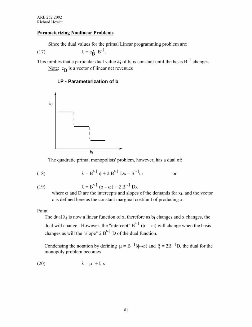
ARE 252 2002 Richard Howitt
Parameterizing Nonlinear Problems Since the dual values for the primal Linear programming problem are: (17) λ = cB' B-1.
This implies that a particular dual value λi of bi is constant until the basis B-1 changes. Note: cB is a vector of linear net revenues
bi
λi
LP - Parameterization of b i
The quadratic primal monopolists' problem, however, has a dual of: (18) λ = B'-1 φ + 2 B'-1 Dx – B'-1ω or (19) λ = B'-1 (φ – ω) + 2 B'-1 Dx where α and D are the intercepts and slopes of the demands for xi, and the vector
c is defined here as the constant marginal cost/unit of producing x. Point The dual λi is now a linear function of x, therefore as bi changes and x changes, the
dual will change. However, the "intercept" B'-1 (φ – ω) will change when the basis changes as will the "slope" 2 B'-1 D of the dual function.
Condensing the notation by defining µ ≡ B–1(φ–ω) and ξ ≡ 2B–1D, the dual for the
monopoly problem becomes (20) λ = µ + ξ x
81

ARE 252 2002 Richard Howitt
Example The following simple Quadratic problem illustrates the nonlinear dual. Min φ 'x + 1/2 x 'Dx Subject to A x ≤ b x ≥ 0
where φ ' = [ ]-8 -6 -4 and D =
4 2 2
2 4 0
2 0 2
and A =
[ ]1 1 2 and b is parameterized over the values 0 → 4.
QP Parameterization - Plot of dual and RHS
1 2 3 40
2
4
6
8
10
λ j
jb
b Values - Series 1
Dua
l Val
ue
5
Comment As one would expect from the equations (19) and (20) on the previous page, the
quadratic dual is a continuous linear function of bj within a basis, since x = B-1b. With a change of basis, the slope of the linear function changes discretely. Equation (19) shows that both the intercept and slope of the dual value function changes with a change in the basis B.
82

ARE 252 2002 Richard Howitt
Incorporating Endogenous Supply and Demand Prices Linear Programs assume constant prices and costs. In reality:
a) Marginal costs are rarely constant.
b) Output prices are only constant for individual firms. Analysis which is performed on a regional, national, or commodity basis should have prices that change with changes in the solution.
CASE: I Changes in Output Price Only
Assuming that we are given, or have estimated the parameters of a linear demand function, we can relate the quantity of output demanded q with its price p.
q = a + Sp where: p and q are vectors of prices and quantities. the parameter ( a ) is a vector of positive slope intercepts. S is a negative definite matrix of demand slopes and cross demand effects.
Note: By definition, a matrix S is negative definite if the scalar product k′Sk < 0 for all non-zero values in a conformable vector k.
Since we are modeling the aggregate outcome of individual farmer behavior, we are interested in the opposite effect – i.e., how output levels q affect the price received. This assumption imples that farmers are so small in their individual output that they are price takers. In addition, for most agricultural crops, the farmer has to commit to purchasing the inputs before it is clear what the price will be at harvest. Therefore we invert the demand function to get it in a price dependent form.
p = -S-1a + S-1q or p = φ + Dq where φ ≡ –S-1a and D ≡ S-1
Assuming a constant yield per acre for the moment , we can replace the output quantity (q ) by the number of acres allocated to a crop (x ) and substitute the resulting expression for price into the objective function. The price endogenous objective function differs with the assumptions on the objectives of the decision maker. There are two main specifications. a) Monopolist (Price Manipulator)
b) Perfect Competition (Price Taker)
83

ARE 252 2002Richard Howitt
84
(a). Monopoly
Assume a monopolist faces a set of linear price dependent demand functions for thevector of outputs x.
(1) Demand System P = φ + Dx (D is a symmetric negative definitive matrix)
If the monopolist has a constant marginal cost of production vector c the net revenueobjective function will be:
(2) Max J = p'x - ω'x substituting in (1)
(3) J = (φ + Dx)'x - ω'x or:
(4) Max J = φ'x + x'Dx - ω'x subject to Ax ≤ b x ≥ 0
Unconstrained Equilibrium
Take the derivative J
x set it = 0 and transpose it. In this problem there are no
binding resources, the constraints are all slack, therefore: Marginal Revenue = Marginal Cost
(5) φ + 2Dx = ω↑ ↑
Vector of Marginal = Vector ofRevenues Marginal Costs
Monopoly rent is defined as the difference between total revenue and total cost.Monopoly rent = p′x – ω′x
= (φ + Dx)′x – (φ + 2Dx)′x↑ ↑p MR since monopolist produces where MR=MC
Monopoly Rent = –x′Dx
Note: The monopoly rent – x′Dx is a positive scalar value since D is a negative definitematrix.

ARE 252 2002Richard Howitt
85
Constrained Monopoly Equilibrium
The monopolist is now constrained by a vector of fixed inputs b and the linear technologymatrix A. The Lagrangian now becomes
(6) Max J = φ′x + x′Dx – ω′x + λ′(b–Ax)
The first order optimum conditions are:
(7)
20JDxAx′′=+−−=
( Set equal to zero)
(8) φ + 2Dx – ω = A′λ
That is, the difference between the marginal revenue and marginal cost of an output is thesum of shadow values of the inputs used to produce it.
Graph for the Single Product xi Unconstrained Constrained
(b) Aggregated Perfectly Competitive Case
Perfect competition is defined by the following unconstrained equilibrium condition.
( 9 ) z
x = 0 (set = 0 and transpose), yields φ + Dx = ω
↑ = ↑ Price Marginal Cost
Constraint
M R
Price
Dual Value
M Cost
X*
M R
X*
M Cost
Price

ARE 252 2002 Richard Howitt
The perfectly competitive objective function is obtained by integrating the optimal marginal condition from (9), namely. ∫ (φ + Dx - ω ) dx = φ′x + 1/2 x′Dx - ω′x Accordingly, we specify a different objective function that satisfies the marginal conditions for unconstrained perfect competition. (10) Max z = (φ + 1/2Dx)'x - ω'x A good question is: Why is the one half in the objective function multiplying the slope parameter ? The answer is that a Perfectly Competitive market is defined by its marginal conditions, so to correctly define the objective function, we have to start with the marginal conditions and derive the objective function. Essentially we have to ask, what objective function would an optimizing decision maker have had to result in these first order conditions ? We therefore start with the marginal conditions and integrate them to obtain the objective function. The Constrained Perfect Competition Problem. (11) Max z = φ'x + 1/2 x'Dx - ω'x Subject to Ax ≤ b x ≥ 0 The perfectly competitive objective function also maximizes the sum of consumer's surplus and producer's quasi-rent (producer surplus) (12) z = (φ + 1/2Dx)'x - ω'x (add and subtract 1/2x′Dx) = (φ + Dx)'x - ω'x - 1/2 x'Dx (substitute in for price p) = p'x - ω'x - 1/2 x'Dx = (P-ω)' x - 1/2 x'Dx Since Price minus Variable Cost is defined as “Quasi Rent” or producer's surplus, the left hand side term (P-ω)' x is equal to quasi rent. Since the marginal cost is defined as a constant value “ω”, the quasi rent only occurs because of the constraint on the amount of product sold. What about the right hand side term - 1/2 x'Dx ? (13) -1/2 x'Dx = 1/2 x'(-Dx) (add and subtract φ ) = 1/2 x'(φ-φ-Dx) (substitute in for price p* ) = 1/2 x'(φ-P*) = consumer's surplus (see figure) Thus equation (9) (a) Satisfies competitive marginal conditions (b) Maximizes aggregate net social benefits.
86

ARE 252 2002 Richard Howitt
Unconstrained perfect Competition Constrained Perfect Competition
PriceC S
X* X*
M C
Demand function φj + dj xj
P S
C S
Constraint
Price = M C
Summary.
Unconstrained Perfect Competition Constrained Perfect Competition Producer Surplus (p.s.) = 0 Producer Surplus (p.s.) = quasi-rent attributed the fixed input bj (pi - ωi) xi Consumer Surplus (c.s.) = 1/2(φi–pi)xi Consumer Surplus (c.s.) = 1/2(φi–pi)xi
CASE II Aggregate Perfect Competition—Endogenous Prices and Costs In this specification the marginal costs is no longer constant and there is a linear supply function (Marginal Cost) as well as endogenous demand prices. Given the price dependent demand function and a linear marginal cost (supply) function below Price = φ + Dx D is negative definite (15) Marginal Cost = α + Γx Γ is positive definite. The unconstrained problem is therefore. (16) Max J = φ′x + 1/2x′Dx – α′x – 1/2 x′Γx
87

ARE 252 2002 Richard Howitt
(17) xJ
δδ = φ′ + x′D – α′ – x′Γ set
= 0
As expected for perfect competition—price = marginal cost. The Interpretation of the Objective Function Trick #1. Add and subtract 1/2x′Dx and 1/2x′Γx to (16) to yield: (18) J = φ′x + x′Dx – α′x – x′Γx – 1/2x′Dx + 1/2x′Γx (19) J = (φ + Dx)′x – (α + Γx)′x – 1/2 x′Dx + 1/2 x′Γx But from (17) we see that the first two terms cancel out (Price = Marginal cost) at the optimum therefore at the optimum the objective function is: (20) J = –1/2x′Dx + 1/2x′Γx From (13) we see that the first term – 1/2 x′Dx is equal to consumer's surplus. The second term is changed by trick #2—factoring out x and adding and subtracting α to yield: (21) 1/2 x′Γx = 1/2 (α + Γx – α)′ x = 1/2 (MC – α) x Since price equals marginal cost, 1/2 x′Γx is one half the area above the marginal cost intercept and below the price line as shown below.
88

ARE 252 2002 Richard Howitt
Perfect Competition–Endogenous Price and Cost
φ
Demand (φj + dj xj )
Supply (αj + γj xj )
Price = MC
α
X*
CASE III Inter-regional Trade Models
Empirical trade models can be solved using this same objective function expanded to several regions. The effect of transport costs and tariffs can be added to the supply functions to solve for changes in trade policies or conditions. The seminal paper in this area is by Takyama and Judge (1964). There are several different ways of setting up the inter-regional trade problem, but the simplest method to show is to extend the quantity dependent supply / demand concept above to J regions that are linked by trade which results in a trading cost of ωij per unit commodity traded from region “i” to region “j”. The resulting problem solves a wide range of trade problems
89

ARE 252 2002 Richard Howitt
Quantity Dependent Optimal Inter-regional Trade Specification
1 1(.) ( 0.5 ) ( 0.5 )
. .
0
J Ij j j j i i i i ij ijj i
i j
i ijj
j iji
ij
Max F d xd xd xs xs c x
s t xs x
xd x
x
φ α γ= =
= + − + −
=
=
≥
∑ ∑
∑
∑
∑∑
The objective function maximizes the definite integral under the demand and supply function for each region in terms of the post trade quantities demanded and supplied in each region. The costs of trading between regions is deducted to yield the net social benefit of trade shown in the two region diagram. The adding up constraints ensure that the quantities demanded and supplied in each region balance. The specification of the regional trade problem is an excellent illustration of the efficiency and beauty of dual specifications. The primal specification above solves optimally, but it is a bit more complicated than needed. Since the decision variable is the quantity of product traded between regions, the cost of trading is explicitly defined in the objective function, and the aggregate quantities are generated by the summing up constraints. An alternative to using quantity dependent supplies and demands, is to formulate the dual of the quantity dependent problem that can be termed the price dependent form. The price dependent specification solves the problem with two simple equations that use the standard quantity dependent demand and supply functions, and instead of solving for i*j quantities traded, the price based model solves for the i + j set of equilibrium prices. The two equations are the producer and consumer surplus objective function, and the first order price condition for trade. Returning to the original quantity dependent demand on page 76 we have: xdj = aj + sj pdj We also define a similar quantity dependent supply function xsi = bi + gi psi
90
ARE 252 2002 Richard Howitt
The Price Dependent Interregional Trade Problem
1 1(.) ( 0.5 ) ( 0.5 )
. .0
J Ij j j j i i i ij i
j i ij
Max F a s pd pd b g ps ps
s tpd ps c
= == + − +
− − ≤
∑ ∑
The quantities traded are generated as the dual values to the ( i * j ) interregional pricing constraints. This is an example of the complementary slackness principle working for us. From the complementary slackness principle we know that if the trade price constraint is slack, that is the supply and transport cost exceed the demand price, then the quantity traded will be zero. The corollary is that the dual value when the trade price constraint is binding is the quantity traded. Note that all the information from the optimal solution of the primal problem is also obtained from solving the simpler dual problem. An empirical example of the Gams code for these problems is found in chapter 10. By running both problems it can be seen that the results are identical.
91

ARE 252 2002 Richard Howitt
92
Calibrating Demands Using Elasticity Estimates Often the modeler is faced with the need to derive parameters for demands and supplies when the only data available is the equilibrium price and quantity in the base year for the model, and an estimate of the elasticity from an previous econometric study. There is a very simple derivation that enables one to calibrate the slope and intercept coefficients using the elasticity. Assume that a demand can be specified as linear in form used above. pd d xφ= + Recall that that demand elasticity is defined as:
q pp q
δηδ
=
If you have a base value for q = 2.9 , p = 173, and the elasticity = -0.6 the values can be substituted in to the above formula to solve for the slope of the demand function
1730.62.9
qp
δδ
− =
The slope of the price dependent linear demand function that results is:
δδpq
= − 99 42.
Substituting this value back into the original price dependent demand equation results in an intercept value of 461.3 The resulting calibrated demand curve that will yield a price of $173 at a quantity of 2.9 and a point elasticity of -0.6 has the form: pd = 461.3 – 99.42 q The concept of calibrating models against prior econometric elasticity estimates is well illustrated in the Central Valley Production Model (CVPM ) that has been developed by S Hatchett in the consulting firm CH2M - Hill. The CVP model is currently used to analyze the economic impacts of large reallocations of water between agricultural, environmental and urban interests in California. The model use both demand, supply and substitution elasticities to reflect the economic impacts of changes in water availability and cost in California.
AE 252 2002 Richard Howitt
VII Incorporating Risk and Uncertainty
In our problem specifications we have implicitly assumed that the parameters in the problem are known and constant. For example, the objective function c'x assumes a deterministic vector c of prices or costs. We can make this more realistic in two ways: a. Assume the elements of c are not known with certainty, but they are stochastic with
known distributions.
c ~ N (_c , Σc)
where Σc is an n x n variance/covariance matrix of revenues.
b.The decision maker's objective function values both the expected return and its variance.
Question
If the vector of net revenues c is distributed c ~ N (_c , Σc), what is the distribution of the
objective function c'x, where x is a non-stochastic vector. Answer Since x is a deterministic linear operator
a. Expected Value E (c'x) = _c 'x
b. Variance of c'x = E c'x - E (c'x)"Squared" Var (c'x) = E [c'x – E (c'x)]' [c'x – E (c'x)] (Inner Product) = E x' [c – E(c)] [c – E(c)]' x (Inner Product of an Outer Product) = x' E[c – E (c)] [ c – E (c)]'x (Taking Expectation of stochastic terms) = x' Σc x (by covariance matrix definition) Point
If c ~ N (_c , Σc) then
c'x ~ N (_c 'x, x'Σcx) where x is deterministic.
If the decision maker is risk neutral, the objective function has _c substituted for c. But
more likely, the decision maker is risk averse.
93
AE 252 2002 Richard Howitt
If the degree of aversion to income variance can be measured by a parameter "ρ" then the problem becomes: max z = –c 'x – ρ x' Σcx ↑ ↑ (expected revenue vector) (variance of revenue) Subject to Ax ≤ b x ≥ 0. The Effect of Uncertainty and Risk Aversion This nonlinear risk cost will have several different effects on the optimal solution of the problem.
(i) The optimal solution will show more diversification to offset risk. (ii) Since the problem is no longer linear in x, some of the xj's may have
interior optima and will not be restricted by binding constraints. In this case, there will be more xj activities than constraints.
(iii) Note that ρ is a scalar, since the variance of a vector product (c'x) is a scalar. "ρ" measures the "cost of risk" to the decision maker. The variance of the return from the portfolio x′Σcx and the expected return –c ′x are both changed by changing the proportions of xi in the portfolio.
The point is demonstrated by focusing on a single xi, and denoting the sum vector
of derivatives that result from the covariance by the short hand expression δδ(var)xi
.
δδzxi
= δδ( ′c xxi
) – ρ δδ(var)xi
= 0 (Set equal to zero for an unconstrained optimum)
∴ ρδ
δ(var)xi
= δ
δ( )′c xxi
∴ ρ = δ
δ( )′c xxi
δδxi
(var) = δ
δ( )(var)
′c x
That is ρ is equal to the marginal rate of tradeoff between expected income and variance at the optimum.
94
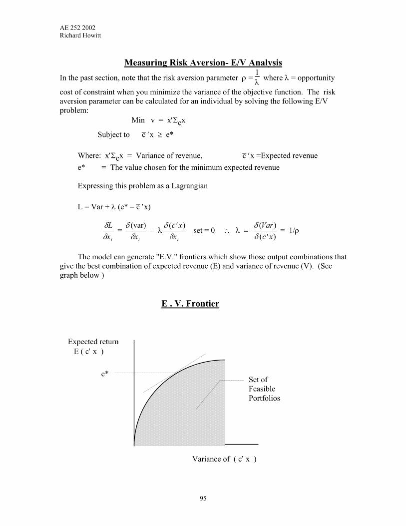
AE 252 2002 Richard Howitt
Measuring Risk Aversion- E/V Analysis
In the past section, note that the risk aversion parameter ρ = 1λ where λ = opportunity
cost of constraint when you minimize the variance of the objective function. The risk aversion parameter can be calculated for an individual by solving the following E/V problem: Min v = x′Σcx
Subject to –c ′x ≥ e* Where: x′Σcx = Variance of revenue, –c ′x =Expected revenue e* = The value chosen for the minimum expected revenue Expressing this problem as a Lagrangian L = Var + λ (e* – –c ′x)
δδLxi
= δδ(var)xi
– λ δδ( )′c xxi
set = 0 ∴ λ = δδ
(( )Varc x′
) = 1/ρ
The model can generate "E.V." frontiers which show those output combinations that give the best combination of expected revenue (E) and variance of revenue (V). (See graph below )
E . V. Frontier
Set of Feasible Portfolios
Expected return E ( c′ x )
e*
Variance of ( c′ x )
95
AE 252 2002 Richard Howitt
The EV frontier is generated by the following steps (1) min var (c′x) s.t. –c ′x ≥ e* for a range of e* values (2) plot results A simple example of the Gams code for the E/V problem is found in chapter 10. Note: There is a linear approximation to the mean/variance objective function called MOTAD. (see Hazell and Norton pp. 86-90). With the growth in nonlinear algorithms and computing power, this linear approximation is rarely needed.
96
AE 252 2002 Richard Howitt
Uncertainty in the Constraints: Chance Constrained Programming
The constraints of a problem sometimes are not known with certainty. Often the quantity available of input resources (bi's) is uncertain, for farming this may be reflected by the distribution of growing season length, rainfall or seasonal labor availability. The aij technological coefficients may also be stochastic, but this more complex case is set aside for the moment. Case Considered
a) Some or all of the right hand side bi's are stochastic. Their distribution is known. b) The problem decision maker has specified that the problem solution must have the
uncertain constraint satisfied for a known proportion (α) of the time. That is the probability that the constraint is satisfied is specified.
Probability Review Any normal random variable can be transformed to a variable that has a "Standard Normal Distribution" -N (0,1). whose cumulative probabilities are calculated and tabulated (z distribution)
if bi ~ N( b_ i, σ
2bi ) then
bi – b_i
σbi ~ N(0,1)
Also the probability that a z distributed random variable exceeds a specified value is equal to one minus the cumulative probability at that value.
Case: A Single Right Hand Side Value bi is Normally Distributed (1) Given the problem Max c′x s.t. Ax ≤ b the ith row in the constraints is written:
(2) ∑j=1
naijxj ≤ bi
But if bi is stochastic and we want this constraint to hold with probability α, it is rewritten as:
(3) Prob
≥ α b a xi j
n
ij j≥ =
Σ1
97

AE 252 2002 Richard Howitt
This is the probability that the constraint is slack, or just holds. Note that the right hand side of the expression in the brackets . is deterministic but changes with changes in x.
a xij j
Step 1 If we require the probability that a normally distributed random variable will be equal
to or bigger than a number we need to calculate a value where cumulative probability is α, our specified level. It is quick and convenient to convert the distribution to an equivalent standard normal and look up the probabilities in a table.
Note: Z tables are usually set up so that: 1) They only tabulate half the distribution, so you have to add or subtract .5 from the
cumulative probability. 2) They give the cumulative probability in the "tail" of the distribution. (4) If the variable zi is distributed zi ~ N(0,1) That is, zi is distributed with a standard normal distribution, the probability that zi ≥ Q is greater than α holds only if Q ≤ kα . Where the cumulative probability (1 – α) is the area under the curve (density
function) in the tail beyond kα.
(1 – ) αα
0kα
Example
0kα 0kαQ
Low Q Value High Q Value
Q
Prob zi ≥ Q > α Prob zi ≥ Q < α
98
AE 252 2002 Richard Howitt
Step 2.
a) Convert the normally distributed bi to an equivalent standard normal distribution, as above.
(5) bi is "standardized" to zi = bi – b
–i
σbi
Since we want to put this "standardized" value into the constraint (3) we have to
perform the same bi standardization transformation on the other ( ∑j=1
naijxj ) side
of the constraint. Applying the transformation to both sides, constraint (3 ) is rewritten for the standard normal distribution as equation (6). Note that the left hand term in the brackets is a random variable, while the right hand term is deterministic.
(6) Prob ≥ α b - b
a x - b
i i
bi
ij jj=1
n
i
biσ σ≥
∑
Note: a) bi – b
–i
σbi ~ N(0,1) That is, it has a standard normal distribution.
b)
∑j=1
naijxj – b
–i
σbi is composed of fixed and known parameter values and thus is
equivalent to the value Q used above. From Step 1 and equation (4) we see that Prob zi ≥ Qi ≥ α , holds only if Qi ≤ kα . Therefore, expression (6) only holds if:
(7)
∑j=1
naijxj – b
–i
σbi ≤ kα
99
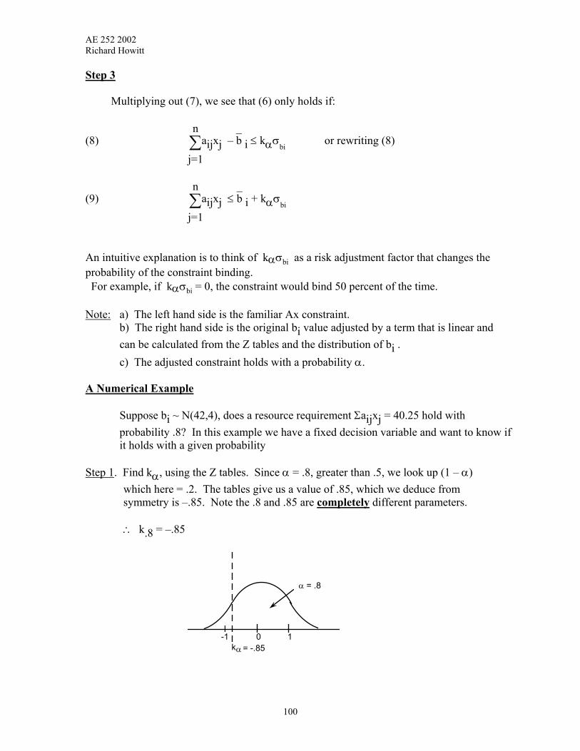
AE 252 2002 Richard Howitt
Step 3 Multiplying out (7), we see that (6) only holds if:
(8) ∑j=1
naijxj – b
– i ≤ kασ
bi or rewriting (8)
(9) ∑j=1
naijxj ≤ b
– i + kασ
bi
An intuitive explanation is to think of kασbi as a risk adjustment factor that changes the probability of the constraint binding. For example, if kασbi = 0, the constraint would bind 50 percent of the time. Note: a) The left hand side is the familiar Ax constraint. b) The right hand side is the original bi value adjusted by a term that is linear and
can be calculated from the Z tables and the distribution of bi . c) The adjusted constraint holds with a probability α. A Numerical Example Suppose bi ~ N(42,4), does a resource requirement Σaijxj = 40.25 hold with
probability .8? In this example we have a fixed decision variable and want to know if it holds with a given probability
Step 1. Find kα, using the Z tables. Since α = .8, greater than .5, we look up (1 – α)
which here = .2. The tables give us a value of .85, which we deduce from symmetry is –.85. Note the .8 and .85 are completely different parameters.
∴ k.8 = –.85
α
0kα
= .8
-1 1= -.85
100

AE 252 2002 Richard Howitt
101
Step 2. Find "Q" using values from the distribution of bi
"Q" =
∑j=1
naijxj – b
–i
σbi =
40.25 – 42 2 = –.875
Step 3. Comparing kα and Q, we see that Q < kα, i.e., –.875 < –.85 ∴ we know that the
constraint value of 40.25 will be satisfied slightly more than 80% of the time. Uncertainty in the Technical “aij “ Coefficients Case a) Individual aij's have a known mean and variance b) Two or more aij's have a non-zero covariance. Result We use the same probability concept as with the bi, but the derivation results in
nonlinear (quadratic) constraints in x. For details see Hazell and Norton pp.107-110. For a more general model specification that combines the mean / variance objective function and chance constraints on the input supply, see Paris (1979) Paris Q. “Revenue and Cost Uncertainty, generalized Mean- Variance, and Linear Complementarity Problem”. A J A E. 61, 2: ( May 1979): 268- 275.

ARE 252 2002 Richard Howitt
VIII An Introduction to Maximum Entropy Measuring Information The PMP cost function in chapter 5 has its quadratic coefficients solved analytically by solving two equations in two unknowns. However, this analytical solution requires that the quadratic cost matrix is specified as strictly diagonal. There is a significant practical problem with the diagonal specification in that is assumes that there are no "cross effects" between the amount of land allocated to crops, apart form the effect on the total land constraint. In economic parlance this assumption requires that there are no substitution or complementarity cost effects between crops grown in the same district or farm. Clearly the almost universal existence of rotations in crop production implies that farmers are well aware of the interdependencies among crops, and use them to stabilize or increase profits. Clearly, the assumption of a diagonal cost matrix is unrealistic. But to calibrate a full matrix of coefficients requires solving an " ill posed" problem in which we are trying to estimate more parameter values than we have data points, an estimation with negative degrees of freedom. As we saw in chapter 2, we cannot solve ill posed problems by inverting matrices. Fortunately there is an alternative method that can obtain parameter estimates for ill posed problems using information theory and the principle of maximum entropy. Claude Shannon was a giant in information theory. In 1948, he published a paper that proposed a mathematical way of measuring information , and started the information revolution. Shannon noted that information is inextricably linked with the probability of an event about which the signal tells us. Clearly a signal that tells us that an extremely unlikely event, such as a bad earthquake in Davis, has gone from a very low probability of happening to a very high probability has a very high information content. Note, we are not even considering whether the event has any particular value associated with it. Likewise a signal that tells us that a very likely (high probability ) event will happen has a low information content. Shannon proposed several axioms that a measure of information must have, and showed that the only measure of information content that satisfied the axioms is if the information content of a signal is: (1) - ln (p) where p is the prior probability of the event happening. Shannnon extended the definition from single probabilities to discrete distibutions and defined the expected information content of a prior distribution Σi pi as the entropy of a distribution: (2) H = - Σi pi ln pi . It follows that a distribution that has a uniform distribution, in which each event is equally likely, has the highest entropy and the lowest information content. Conversely, a distribution that puts a weight of one on a single outcome and zero on the rest, has an entropy of zero. Remember that, counterintuitively, a distibution that shows that a given
102

ARE 252 2002 Richard Howitt
event will occur with probability one, has the highest information content ( lowest entropy). If we specify a set of discrete values over the feasible range of a parameter value termed the "support set or space" then multiplying each support value by its associated probability yields and expected parameter estimate, and there is an entropy value for the distribution associated with the parameter value. However, as one would expect with an ill posed problem, there is an infinite set of probabilities that will yield any given parameter value. We have to use the entropy criteria to choose a unique distribution fomr among the infinite set of feasible distributions. Jaynes , another information pioneer, showed that the distribution with the highest entropy can occur in the most number of ways. The concept of "multiplicity" is similar to frequency or maximum likelihood in conventional estimators. Essentially the distribution with the maximum entropy is the "best" estimator. Maximizing entropy also has another fine property, in that the entropy function in equation (2) has a unique solution at the maximum. Thus by defining a support space for our parameter and so9lving for the maximum entropy distribution that has an expected value consistent with the data, we can get a unique solution to the ill posed problem, and estimate more parameters than we have observations! The “Loaded” Dice Example Here we se how we intuitively calculate six parameters ( probabilities) from a single data observation. Jaynes in his 1963 Brandeis lectures on maximum entropy used the example of a game using a six sided dice with the usual values from 1 – 6. Suppose that you know the average value of a large number of independent rolls of the dice. For a given mean value there are an infinite number of combinations of the six probabilities that could have generated the mean value. The problem is ill posed because we are given one data point, the mean value, and we have to estimate six probabilities. The only structural constraint that we have is that the probabilities have to add to one. Think about a game in which your opponent produces a dice and suggests that it is rolled twenty times, and if the average score is above 4 you win, and if the average score is below 3 they win. With a “fair dice” in which we assume that the probability of each side coming up is even, this is a fair game. If you notice that the rolls of the dice come up consistently with 1,2,or 3, you will alter your initial assumption that the dice is fair, and assume that your opponent is cheating with a dice loaded to favor the low scores. You have just performed an ill-posed estimation of the probabilities. Using the principle of multiplicity, the distribution that maximizes the entropy is the most likely to be probabilities underlying the dice. If we define the score values as xi, the dice problem is specified as:
Max H = - Σi pi ln pi (6)
subject to Av Score = Σi xi pi
Σi pi = 1, pi ≥ 0
103

ARE 252 2002 Richard Howitt
The Gams solution to the dice problem is in the website Gams folder. The ME probability results for a range of average scores from 1.5 to 5.5 is plotted below.
Max Entropy Dice probabilities
0
0.1
0.2
0.3
0.4
0.5
0.6
0.7
1 2 3 4 5 6
Dice Values
Ad=1.5
AD = 2.5
AD = 3.5
AD = 4.5
AD = 5.5
The entropy value for different average scores is plotted below, note the unique maximum value.
ENTROPY
-0.2
0
0.2
0.4
0.6
0.8
1
1.2
1.4
1.6
1.8
2
1 1.5 2 2.5 3 3.5 4 4.5 5 5.5 6
Value of Average Draw
Entr
opy
104
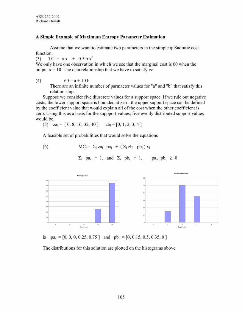
ARE 252 2002 Richard Howitt
A Simple Example of Maximum Entropy Parameter Estimation Assume that we want to estimate two parameters in the simple qu8adratic cost function: (3) TC = a x + 0.5 b x2 We only have one observation in which we see that the marginal cost is 60 when the output x = 10. The data relationship that we have to satisfy is: (4) 60 = a + 10 b.
There are an infinite number of parmaeter values for "a" and "b" that satisfy this relation ship.
Suppose we consider five diuscrete values for a support space. If we rule out negative costs, the lower support space is bounded at zero. the upper support space can be defined by the coefficient value that would explain all of the cost when the other coefficient is zero. Using this as a basis for the suppport values, five evenly distributed support values would be.
(5) zai = [ 0, 8, 16, 32, 40 ]. zbi = [0, 1, 2, 3, 4 ] A feasible set of probabilities that would solve the equations (6) MCj = Σi zai pai + ( Σi zbi pbi ) xj
Σi pai = 1, and Σi pbi = 1, pai, pbi ≥ 0
Ad Hoc values for pb
0
0.1
0.2
0.3
0.4
0.5
0.6
0 1 2 3 4
Support values
Ad Hoc pa values
0
0.1
0.2
0.3
0.4
0.5
0.6
0.7
0.8
0 8 16 32 40
Support values
is pai = [0, 0, 0, 0.25, 0.75 ] and pbi = [0, 0.15, 0.5, 0.35, 0 ] The distributions for this solution are plotted on the histograms above.
105

ARE 252 2002 Richard Howitt
The Maximum Entropy Solution The maximum entropy problem that solves for the two distributions that are most
likely to have generated a marginal cost of 60 for an output of 10 is: Max H = - Σi pai ln pai - Σi pbi ln pbi (6)
subject to MCj = Σi zai pai + ( Σi zbi pbi ) xj
Σi pai = 1, and Σi pbi = 1, pai, pbi ≥ 0 The maximum entropy (ME) solution to this problem is plotted on the histograms below. Clearly the ME solution satisfies the data constraint without having to use such specialized, and unlikely, distributions as the ad hoc solution above.
Parameter "a"
0
0.05
0.1
0.15
0.2
0.25
0.3
0.35
0.4
0.45
0.5
0 8 16 32 40
Support values
Max Entropy for Parameter B
0
0.05
0.1
0.15
0.2
0.25
0.3
0.35
0.4
0.45
0.5
0 1 2 3 4
The expected parameters that result from these two calculations are shown below Ad Hoc Values Maximum Entropy E(a) 38.0 30.217 E( b) 2.2 2.978
106
ARE 252 2002 Richard Howitt
Defining the Support Space Values ( Z values) Since the z values are “priors” on the parameters that we want to reconstruct they can have a strong influence on the resulting parameters. We need to be aware that the defined z values must be: 1. Feasible for the data constraints that we are going to impose on the support space. 2. Neutral in their effect on the estimate unless we have information that we want to
incorporate in the priors. Feasible Supports. In the simple parameter and dice example the z values of the dice are clear, and for the cost parameters they were glossed over. When defining a system for generating z values for different models and crop components in the models we need a more formal approach. Feasible z values are generated by defining the z values ( say five) as being the product of a single centering parameter value and five z weight parameters. zval( j, p) = zwgt(p)* cval(j). The centering cval(j) is an empirical value the modeler calculates will be feasible for the data set imposed on it. For example, if we are reconstructing a PMP cost function matrix as a function of the acreage planted of a crop, then a feasible value for the marginal cost coefficient is the average cost divided by the base acres. Non-Informative z values The zwgt(p) parameters can be thought of as spreading the cval(j) value across a feasible range for estimation. For a diagonal cost parameter that is strictly positive, the range may go from 0, 0.5, 1.0, 1.5, 2.0. For an off-diagonal parameter the cval(j) weight will be reduced, possibly to 0.25 the diagonal weight and centered on 0, with weights of –1.5, -0.75, 0.0, 0.75, 1.5.. This system of generating z values is designed to automatically generate a set of feasible but noninformative prior z values. Informative Prior z values. In the Yolo example the z values on the cost slope parameters are defined to be informative, in that their centering value is defined by the model parameters and a prior elasticity value. The elasticity value is entered in the same manner as in the PMP elasticity calibration, and forms a stronger basis for the defined z values. Note this elasticity is based on “scalar” reasoning in the calculation is based on single coefficients and ignores the effect of the off diagonal coefficients and resource constraints, however, as can be seen from the empirical elasticity test, they do give the model an operating range of elasticities.
107

ARE 252 2002 Richard Howitt
Adding Curvature Conditions by Cholesky Decompositions To ensure that the resulting matrix PMP model converges to a stable solution the second order conditions require that the Hessian of the cost function is negative definitive. Since the Hessian is the Zeta matrix, this requires that Zeta is positive definite. Diewert shows that a necessary condition for a matrix to be positive definite is that the diagonal elements of its Cholesky decomposition matrix are positive. What is a Cholesky decomposition ? Judd(1999) says that we can think of a Cholesky decomposition as being the “square root” of a matrix. The C matrix is a lower triangular matrix L that when post multiplied by its transpose yields the original matrix. If Z = L L’ then L is the Cholesky decomposition.
If Z is a 3 x 3 matrix. 11 12 13
21 22 23
31 32 33
z z zZ z z z
z z z
=
The Cholesky decomposition 11
21 22
31 32 33
0 00
lL l l
l l l
=
and
11 11 11 21 11 31
21 11 21 21 22 22 21 31 22 32
31 11 31 21 32 22 31 31 32 32 33 33
l l l l l lZ L L l l l l l l l l l l
l l l l l l l l l l l l
′= = + + + + +
This latter expression results in two sets of equations for the diagonal and off-diagonal elements of Zeta.
21 1
j jjj jk ij ik jkk kz l and z
= == =∑ ∑ l l
by adding these equations as constraints on the entropy problem and constraining the diagonal Cholesky terms to be greater than zero ( here > 0.001 ) we can impose curvature conditions on the Zeta matrix that ensures that the simulated problem will satisfy the second order conditions. The program that implements a ME estimate of the PMP cost matrix for the Yolo model is found in the Gams folder on the website.
108

ARE 252 2002 Richard Howitt
Reconstructing Production Function Models We may have "n" observations over time on production units. For the time being, we
will simplify the problem to a single observation of a unit that produces "j" crops each of which has "i" inputs. There is an input subset of restricted, but allocatable inputs such as land or irrigation water. The data set consists of observations on crop price, input price, crop yield, and input use by crop. This data set can be used to define the implicit Leontieff matrices and specify the following calibrated linear programming problem.
(1)
.
0
j j j j ij i ij
j
jMax p y x a xs t Ax b
I x xx
ω
ε
Σ − Σ
≤≤ +≥
%
The first set of allocatable resource constraints generate the shadow values for those constraints that influence the observed crop and input allocation. The perturbed upper and lower bound calibration constraints ensure that the crop allocation is within ε of the observed data, and in addition, provide measures of the rotational cost interdependence between the crops based on the equi-marginal principle for land allocation.
Before the ME reconstruction program is run, support values have to be defined for each parameter and error term. To ensure that the set of support values spans the feasible solution, we define the support values as the product of a set of five weights and functions of the average Leontieff yield over the data set, and for a particular crop/input combination. The support values for the error terms are defined by positive and negative weights that multiply the left-hand side values of the equation.
Curvature is added by solving for the parameters of the Cholesky decomposition of the quadratic matrix L where Z= LL′, and constraining the diagonal Cholesky parameters to be nonnegative, for details see (Paris & Howitt 1999). The quadratic production function for a single crop j as a function of i inputs is defined as:
jjjj xZxxy ′−′= 5.0α
The ME reconstruction problem for a single crop with "i" inputs becomes:
109

ARE 252 2002 Richard Howitt
,1,1
/]**)]*(*)*([([*
]*)]*(*)*([[*:
lnln
,,,
,,,,,,,,,,
,,,,,,,,,,
,,,,,,,,,
=Σ=Σ
ΣΣΣΣ−Σ=
ΣΣΣ−Σ=
−Σ+−Σ
piiippip
landiiipiiipiiippiiipiiipiiipipip
iipiiipiiippiiipiiipiipipipi
piiipiiipiiipipipi
plpa
xxxzlplzlplzapayld
xzlplzlplzapashtoSubject
plplpapaMax
The objective function is the usual sum of the entropy measures for the two sets of parameters for the Cholesky decomposition of the quadratic matrix and the vector of linear terms. The first equations are the first order conditions that set the cost share equal to the marginal physical product. If some inputs are restricted and the PMP calibration stage is used, the input cost in the share equation will include the resulting shadow values as well as the nominal input price.
The second set of equations fit the production function to the observations on average yield. While it is not normal in econometric models to include average product equations, the information in this constraint is particularly important for two reasons. First, information on yields is likely to be the most precisely know by farmers. Second, while the marginal conditions are essential for behavioral analysis, policy models also have to accurately fit the total product to be convincing to policy makers and correctly estimate the total impact on the environment and the regional economy of policy changes. Fitting the model to the integral as well as the marginal conditions improves the policy precision of the model.
The production function parameters are calculated from the entropy results for each crop as:
)]()([ 2,2,,2,,2,2,
,,
iiiiiippiipiipiiii
pipipi
zlplzlplzeta
zapa
Σ∗ΣΣ=
∗Σ=α
The quadratic production problem is defined as:
jjjjijj
ij
iijj
ijjijijjjj
xZxxxfwhere
x
bxtosubject
xxfpMax
′−′=
≥
≤Σ
Σ−Σ
5.0)(
0
)(
α
ω
110
ARE 252 2002 Richard Howitt
Note that the production technology in the objective function and constraints is no longer Leontieff.
Calculating Comparative Static Parameters for the Model
The quadratic production function model has convenient properties for calculating
policy parameters. Note that the Hessian of the constrained profit function above is simply:
2
2ij
Zx
δδΠ=
Calculating the Derived Demands for Inputs
For simplicity, we will use the unconstrained profit function for a single crop.
ω
α
ωα
αω
ωαδδ
ωα
jj
j
j
j
j
jj
Gax
isjcroponbaseddemandsinputofsystemthe
Zaerceptsofvectortheandp
ZGslopesdemandofmatrixtheDefine
pZZx
pxZ
xZpx
xxZxxp
+=
=
=
−=
−=−
=−−′=Π
′−′−′=Π
−
−
−−
*
1
1
11*
:
int
1
0)(
)5.0(
From the above equations, it is clear that if we can invert the Hessian of the profit function ( Z-1 ) we can calculate the derived demand for each input for each crop as a linear function of input and output price.
Note (i) That x* is an i x 1 vector of the optimal inputs for crop j, and aj is an i x1
vector of intercept terms and Gj is an i x i matrix of derived demand slopes (ii) That the demand for a given input i used in crop j is a function of the prices of
the other inputs as well as its own price.
111
ARE 252 2002 Richard Howitt
The elasticity of demand is based only on the “own price” effect, thus we need to get Gams to only use the ith diagonal elements of DSj
The elasticity of the input demand follows directly :
*,,i
iiijij x
GiselasticityThe ωη =
This elasticity is based on a single crop. For the usual multi-output case we weight the individual crop contribution by their relative resource use to arrive at a weighted elasticity for the resource.
Calculating Supply Functions and Elasticities Since production is a function of optimal input allocation and we now have the input
demands as a function of input and output price, we can derive the output supply function by substituting the optimized input derived demands into the production function and simplify in terms of the output price. Going back to the derived demand and production function formulae:
****
11*
5.0 xZxxy
and
pZZx
j
j
′
−−
−′=
−=
α
ωα
′
−=
′−′=
−′−−−′=
=
−
−−
−−−
ppZ
ppy
rZrZyyieldstermsrandcollectingandoutgmultiplyin
rZZZrrZyrandvectorsthegU
prDefining
II
j
ii
ωωωωα
αα
ααααα
α
ω
......5.0ˆ
5.05.0
)()(5.0)(sin
111*
11*
111*
Substituting the expression for y* into the supply elasticity formula, and separating
out “ω” and “p” we get the supply elasticity expression:
jsj yp
Z ααη15.0 −′
=
112

ARE 252 2002 Richard Howitt
Calculating Elasticities of Input Substitution There are many elasticities of substitution with different advantages and
disadvantages. To demonstrate that we can obtain crop and input specific elasticities of substitution we use the classic Hicks elasticity of substitution defined by Chambers in (Applied Production Analysis, 1988) on page 31 as:
sderivativearefandfwherefffffffxx
fxfxffxxfy
iji
I
)2()(
)....(
21222112
221121
2211212,1
1*
+−+−
=
=
σ
Output from the Yolo Model
---- 324 PARAMETER DIFF PERCENT DIFFERENCE IN INPUT LAND WATER LABOR R1.ALFA 0.0238947 0.0238946 0.0238946 R1.WHEAT -0.0099991 -0.0099990 -0.0099989 R1.CORN -0.0099990 -0.0099990 -0.0099990 R1.TOM -0.0099990 -0.0099990 -0.0099990 ---- 324 PARAMETER YDIFF PERCENTAGE DIFFERENCE IN YIELD ALFA WHEAT CORN TOM R1 -2.54829E-8 5.558568E-8 -1.88046E-8 -6.03031E-9 ---- 324 PARAMETER SUPELAS SUPPLY ELASTICITY ALFA WHEAT CORN TOM R1 1.8559458 0.8040508 1.0985663 0.5755326 ---- 324 PARAMETER DDELAS CROP SPECIFIC INPUT DEMAND ELASTICITY LAND WATER LABOR R1.ALFA 2.5277203 1.2055752 1.3689239 R1.WHEAT 2.1832609 0.6338516 0.3691518 R1.CORN 2.3500945 1.0376875 0.5785391 R1.TOM 1.0477321 0.1712690 1.6733499 ---- 324 PARAMETER DEMELAS AGGREGATE INPUT DEMAND ELASTICITY LAND WATER LABOR R1 2.0916067 0.8465534 1.4426146
113

ARE 252 2002Richard Howitt
114
---- 324 PARAMETER SUB ELASTICITY OF SUBSTITUTION
WATER LABORALFA .LAND 1.3291195 1.2590338ALFA .WATER 1.2621399WHEAT.LAND 0.8346119 0.4626905WHEAT.WATER 0.4797180CORN .LAND 1.2829549 0.7437865CORN .WATER 0.7369215TOM .LAND 0.1828788 1.3330871TOM .WATER 0.1800782
---- 324 PARAMETER ZETA PROD MATRIX
LAND WATER LABORALFA .LAND 0.0020656 -0.0000580 -0.0000613ALFA .WATER -0.0000580 0.0001221 0.0000016ALFA .LABOR -0.0000613 0.0000016 0.0000257WHEAT.LAND 0.0011258 0.0000408 0.0000573WHEAT.WATER 0.0000408 0.0003063 0.0000297WHEAT.LABOR 0.0000573 0.0000297 0.0002101CORN .LAND 0.0022263 -0.0000174 0.0000227CORN .WATER -0.0000174 0.0002478 0.0000130CORN .LABOR 0.0000227 0.0000130 0.0001730TOM .LAND 0.0295139 0.0023333 0.0000889TOM .WATER 0.0023333 0.0036581 0.0000757TOM .LABOR 0.0000889 0.0000757 0.0000135
---- 324 PARAMETER ALPHA PROD LINEAR
LAND WATER LABORR1.ALFA 2.1538230 0.4178334 0.1905927R1.WHEAT 1.5242699 0.5242465 0.3938534R1.CORN 1.6476534 0.3968946 0.2847649R1.TOM 16.8443240 4.6199548 0.4301530
For further reading see: Golan, Judge & Miller “Maximum Entropy Econometrics” Wiley 1996 Mittlehammer, Judge & Miller “Econometric Foundations” 2000. Paris & Howitt AJAE 80: Feb 1998, 124- 138

ARE 252 2002 Richard Howitt
Using Alternative Functional forms for the Production Function
Throughout this analysis we have used the quadratic production function. Two other functional forms that are widely used are the Generalized Leontieff and Translog production functions. As would be expected, the ME empirical reconstruction methods outlined in this chapter apply equally well to these production functions.
For illustration, I show the production surface for all three production specifications for the Yolo model simplified to the two inputs of land and water.
115

ARE 252 2002 Richard Howitt
116

ARE 252 2002 Richard Howitt
IX Nonlinear Optimization Methods
Mathematics For Nonlinear Optimization
Concave Functions and Convex Sets Concave Function A function f(x) defined on a convex set Ω is strictly concave if for every x1 , x2 ∈Ω and every λ, 0 ≤ λ ≤ 1 f(λ x1 + (1-λ) x2 ) > λf(x1 ) + (1-λ) f(x2 ) The tangent line of a scalar valued function f(x) at x1 is f(x1 ) + f ′(x1 ) (x2 – x1 )
Tangent on a Concave Function
x1 x
f(x )1
f(x)
f(x)
f(x1) + f′(x1)(x2 – x1)
It follows that the tangent plane for a vector valued function f(x),at a point in n space , say x1 can be expressed as f(x1 ) + ∇f(x1 )(x2 – x1 ) for x2 ∈ Rn.
117
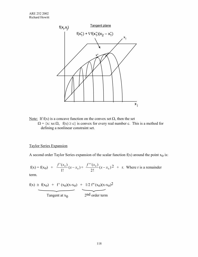
ARE 252 2002 Richard Howitt
f(x) = f(xo) + + ′ ′
−f x
x x( )!
(002) 2 + r. Where r is a remainder
term.
xi
Tangent plane
x*
x j
f(xi,xj)f(x*1) + ∇f(x*1)(x2 – x*1)
Note: If f(x) is a concave function on the convex set Ω, then the set Ω = x: x∈Ω, f(x) ≥ c is convex for every real number c. This is a method for
defining a nonlinear constraint set. Taylor Series Expansion A second order Taylor Series expansion of the scalar function f(x) around the point xo is:
′−
f xx x
( )!
( )001
f(x) ≅ f(xo) + f ′ (xo)(x-xo) + 1/2 f ′′ (xo)(x-xo)2 Tangent at x0 2nd order term
118

ARE 252 2002 Richard Howitt
Taylor Series Expansion of f(x) at x0
f( x )
½ f ′′(x0 ) ( x1 - x0 )2
Tangent Line f(x0 ) + f ′(x0) ( x1 - x0
f( . )
f( x1 )
f( x0 )
x0 x1 Matrix Derivatives For example, for the Linear form:
If L(x) = c′x then δδL x
x( ) = c′,
and for the Quadratic form:
If Q(x) = x'Ax then δδQ x
x( ) = 2x'A,
In both cases the derivative of a scalar with respect to a column vector is a row vector. The Gradient Vector (∇f(x)) A second convention is that the derivative of a scalar with respect to a column (row) vector is a row (column) vector. Thus, if the scalar y is a differentiable function of the
column vector x, the vector of partial derivatives δδ
yxi
is a row vector called the Gradient
vector. For example, if an objective function is a scalar value which is a nonlinear function of n variables.
y = f(x) = f(x1 , x2 , ..., xn)
119

ARE 252 2002 Richard Howitt
then the vector of first order partial derivatives, the gradient vector, is the row vector
∇f(x) ≡ δδf x
x( ) = δ
δδδ
δδ
fx
fx
fxn
(. ),
(.) (. )
1 2
L
Inner Products Because we use inner products a lot we will adopt a new clearer notation. Inner product of two vectors a'b = scalar; will now also be denoted < > a,b = scalar. Thus the familiar objective function c'x = z can be written < > c,x = z.
Hessian and Jacobian Matrices The derivative of the gradient vector with respect to the n×1 column vector x is the n×n Hessian matrix:
δδ
2
2
f xx
( ) = δδ
δδxf x
x( )
=[ ]
δδ
δδ δ
δδ δ
δδ δ
δδ
δδ δ
δδ δ
δδ δ
δδ
2
12
2
1 2
2
1
2
2 1
2
22
2
2
2
1
2
2
2
2
f xx
f xx x
f xx x
f xx x
f xx
f xx x
f xx
f xx x
f xx
n
n
n n n
( ) , ( ) ( )
( ) , ( ) ( )
( ) , ( ) ( )
LL
LL
M
LL
For example, the Hessian matrix of the quadratic form x'Ax is 2A. Jacobian matrix: Similarly the derivative of the column vector of m functions: gi = gi (x), where each function depends on the n×1 column vector x, with respect to x is the m×n Jacobian matrix:
120

ARE 252 2002 Richard Howitt
δδg x
x( ) =
g gx
. . .gx
gx
gx
. . .gx
.
.
.gx
gx
. . .gx
1 1
2
1
n
2
1
2
2
2
n
m
1
m
2
m
n
δδ
δδ
δδ
δδ
δδ
δδ
δδ
δδ
δδ
x1
.
Taylor Series Expansion of a Vector Function
We can now use gradients, Hessians, and the scalar Taylor series to approximate functions of vectors. Suppose f(x) is a function of the n×1 vector x. Given some vector of initial values xo we can expand around this vector to approximate the functional value of some other vector x.
f(x) = f(xo) + < ∇f(xo), (x-xo)> + 1/2 (x-xo)´ Hxo (x-xo) + ro where ∇f(xo) is the Gradient of f(x) at xo Hxo is the Hessian of f(x) at xo (x-xo) is an n by 1 vector of the differences between x and xo. ro is the remainder term of the expansion that could be reduced by
Definite Quadratic Forms. Some quadratic forms have the property x'Ax > 0 for all x except x = 0; some are
negative for all x except x = 0. Positive Definite Quadratic Form: The quadratic form x'Ax is said to be positive
definite if it is positive (>0) for every x except x = 0. Positive Semidefinite Quadratic Form: The quadratic form x'Ax is said to be
positive semidefinite if it is non-negative (≥0) for every x, and there exist points for which x'Ax = 0 and x ≠≠ 0 Negative definite and semidefinite forms are defined by interchanging the words "negative" and "positive" in the above definitions. If x'Ax is positive definite (semidefinite), then x'(-A)x is negative definite (semidefinite).
121

ARE 252 2002 Richard Howitt
An Introduction to Nonlinear Optimization
Some Non Linear Programming (NLP) Definitions The Standard N.L.P. Problem Minimize f(x) where x = nx1 vector Subject to x ∈ Ω and where Ω denotes the feasible solution set. Ω ∈ Rn or a subset of Rn. Note: The objective function or the solution set are no longer defined by linear functions. Local Minima A point x* ∈ Ω is a local minimum of f(x) on Ω if there is a small distance ε such that f(x) > f(x*) for all x ∈ Ω within the distance ε of x*. Verbally "The objective function increases in all directions, therefore we are at the optimum point for a minimization problem." Global Minima A point x* ∈ Ω is a global minimum of f(x) on Ω if f(x) > f(x*) ∀ x ∈ Ω The aim is to set criteria for a computer program to perform a systematic search over a mathematical surface. As in finding your way to a location, good directions will give you a sequence to follow. In each sequence or step you need to know the direction "d" to proceed, and how far "α" to go in that direction. Feasible Directions Along any given single direction "d" the objective function f(x) is a function of the distance moved in a direction. Note any direction in Rn is an n dimensional vector. Definition For x ∈ Ω, d is a feasible direction at xo if there exists a scalar α > 0,
such that (xo + α d) ∈ Ω for all α, 0 ≤ α ≤ α- . i.e. A particle can move in direction “d “ for a distance α ≤ α- without leaving the feasible set Ω.
122
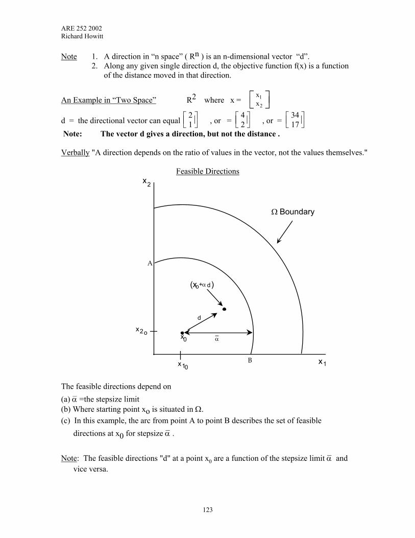
ARE 252 2002 Richard Howitt
Note 1. A direction in “n space” ( Rn ) is an n-dimensional vector “d”. 2. Along any given single direction d, the objective function f(x) is a function
of the distance moved in that direction.
An Example in “Two Space” R2 where x = 1
2x x
d = the directional vector can equal
21 , or =
42 , or =
3417
Note: The vector d gives a direction, but not the distance . Verbally "A direction depends on the ratio of values in the vector, not the values themselves."
Feasible Directions
x2
x o2
x1
Ω Boundary
x0
x10
d
α(xo d+ )
α–
A
B
The feasible directions depend on (a) α– =the stepsize limit (b) Where starting point xo is situated in Ω. (c) In this example, the arc from point A to point B describes the set of feasible
directions at x0 for stepsize α– . Note: The feasible directions "d" at a point x0 are a function of the stepsize limit α– and
vice versa.
123
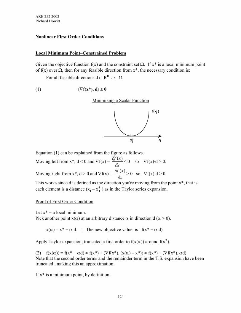
ARE 252 2002 Richard Howitt
Nonlinear First Order Conditions Local Minimum Point–Constrained Problem Given the objective function f(x) and the constraint set Ω. If x* is a local minimum point of f(x) over Ω, then for any feasible direction from x*, the necessary condition is: For all feasible directions d ∈ Rn ∩ Ω (1) ⟨∇f(x*), d⟩ ≥ 0
Minimizing a Scalar Function
f(x )i
x*i xi Equation (1) can be explained from the figure as follows.
Moving left from x*, d < 0 and ∇f(x) = δδxf x( ) < 0 so ∇f(x)·d > 0.
Moving right from x*, d > 0 and ∇f(x) = δδxf x( ) > 0 so ∇f(x)·d > 0.
This works since d is defined as the direction you're moving from the point x*, that is, each element is a distance (xi – x*i ) as in the Taylor series expansion. Proof of First Order Condition Let x* = a local minimum. Pick another point x(α) at an arbitrary distance α in direction d (α > 0). x(α) = x* + α d. ∴ The new objective value is f(x* + α d). Apply Taylor expansion, truncated a first order to f(x(α)) around f(x*). (2) f(x(α)) = f(x* + αd) ≈ f(x*) + ⟨∇f(x*), (x(α) – x*)⟩ ≈ f(x*) + ⟨∇f(x*), αd⟩ Note that the second order terms and the remainder term in the T.S. expansion have been truncated , making this an approximation. If x* is a minimum point, by definition:
124
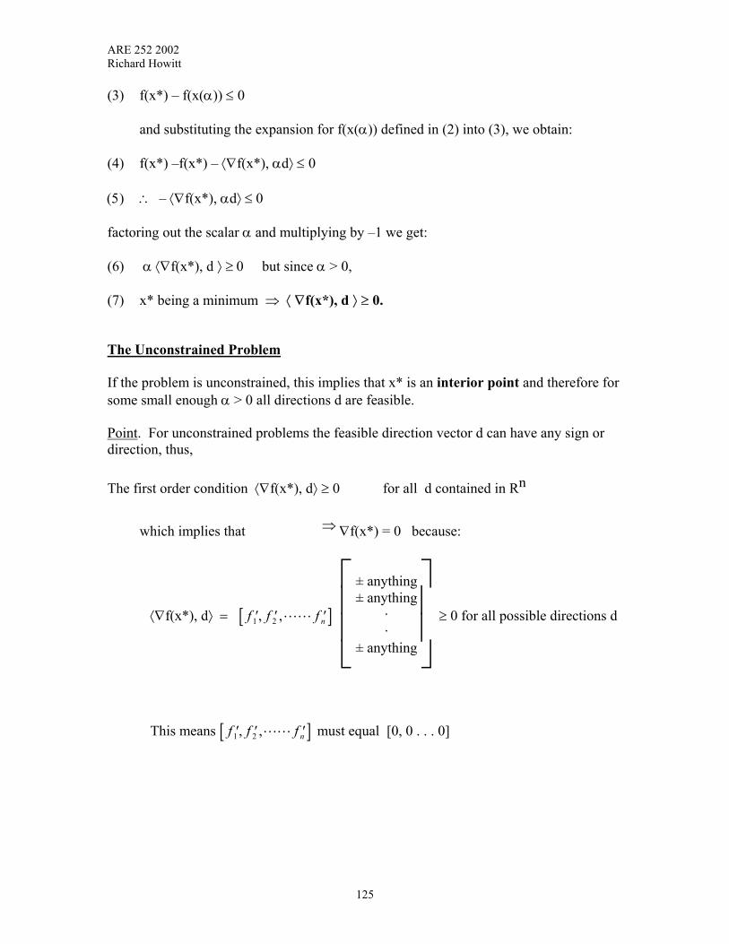
ARE 252 2002 Richard Howitt
(3) f(x*) – f(x(α)) ≤ 0 and substituting the expansion for f(x(α)) defined in (2) into (3), we obtain: (4) f(x*) –f(x*) – ⟨∇f(x*), αd⟩ ≤ 0 (5) ∴ – ⟨∇f(x*), αd⟩ ≤ 0 factoring out the scalar α and multiplying by –1 we get: (6) α ⟨∇f(x*), d ⟩ ≥ 0 but since α > 0, (7) x* being a minimum ⇒ ⟨ ∇f(x*), d ⟩ ≥ 0. The Unconstrained Problem If the problem is unconstrained, this implies that x* is an interior point and therefore for some small enough α > 0 all directions d are feasible. Point. For unconstrained problems the feasible direction vector d can have any sign or direction, thus, The first order condition ⟨∇f(x*), d⟩ ≥ 0 for all d contained in Rn which implies that ⇒ ∇f(x*) = 0 because:
⟨∇f(x*), d⟩ = [ ]
± anything± anything
··
± anything
≥ 0 for all possible directions d ′ ′ ′f f f n1 2, ,LL
]′ ′ ′f f f n1 2, ,LL
This means [ must equal [0, 0 . . . 0]
125

ARE 252 2002 Richard Howitt
Example A. Unconstrained Problem Min f(x1 , x2 ) = 22211
22 3xxxxx −+− There are no constraints therefore the feasible region is the whole of “ two space ” on the real line in symbolic terms: Ω = R2
F.O.C ∇f(•)′ = 0
f(x)x
f(x)x
1
2
δδ
δδ
= set
0
0
Solving the gradient equations yields: ∴ 2x1 – x2 = 0 ∴ x1 = 1/2 x2 -x1 + 2x2 = 3 and -x1 + 4x1 = 3 ∴ solving for x
1 and x
2 we get x1 = 1 x2 = 2
Try substituting this into f(x1 , x2 ) and check other values. Example B. Constrained Optimization Min f(x1,x2) = x2
1 – x1 + x2 + x1 x2
subject to x1 ≥ 0 and x2 ≥ 0
Problem B has a global minimum at x =
0
1
2
x = 1/ 2
Do the constrained first order conditions hold at this point? check FOC ∇f(x*) = 1 2 1 [ ] 2x - 1 + x , x + 1
[ ] [ ]∆x = anywhere
Substituting the numerical x1 =0.5 and x
2 = 0 for x
1 and x
2 in the equation yields
the gradient at the x values of [0.5, 0] of [ ]0, 3/2 Now we pick a small stepsize α, say 1/10 ∴ at x* the feasible directions given the constraints and the initial values are:
d = ∆x = positive values only2
1
126
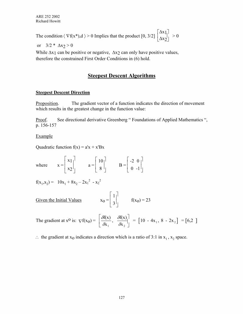
ARE 252 2002 Richard Howitt
The condition ⟨ ∇f(x*),d ⟩ > 0 Implies that the product [0, 3/2]
∆x1
∆x2 > 0
or 3/2 * ∆x2 > 0 While ∆x1 can be positive or negative, ∆x2 can only have positive values, therefore the constrained First Order Conditions in (6) hold.
Steepest Descent Algorithms Steepest Descent Direction Proposition. The gradient vector of a function indicates the direction of movement which results in the greatest change in the function value: Proof. See directional derivative Greenberg “ Foundations of Applied Mathematics “, p. 156-157 Example Quadratic function f(x) = a'x + x'Bx
where x =
x1
x2 a =
10
8 B =
-2 0
0 -1
f(x1,x2) = 10x1 + 8x2 – 2x1
2 - x22
Given the Initial Values xo =
1
3 f(xo) = 23
The gradient at xo is: ∇f(xo) = f(x)x
, f(x)x
1 2
δδ
δδ
= [ ] 10 - 4x , 8 - 2x 1 2 = [ ]6,2
∴ the gradient at xo indicates a direction which is a ratio of 3:1 in x1 , x2 space.
127
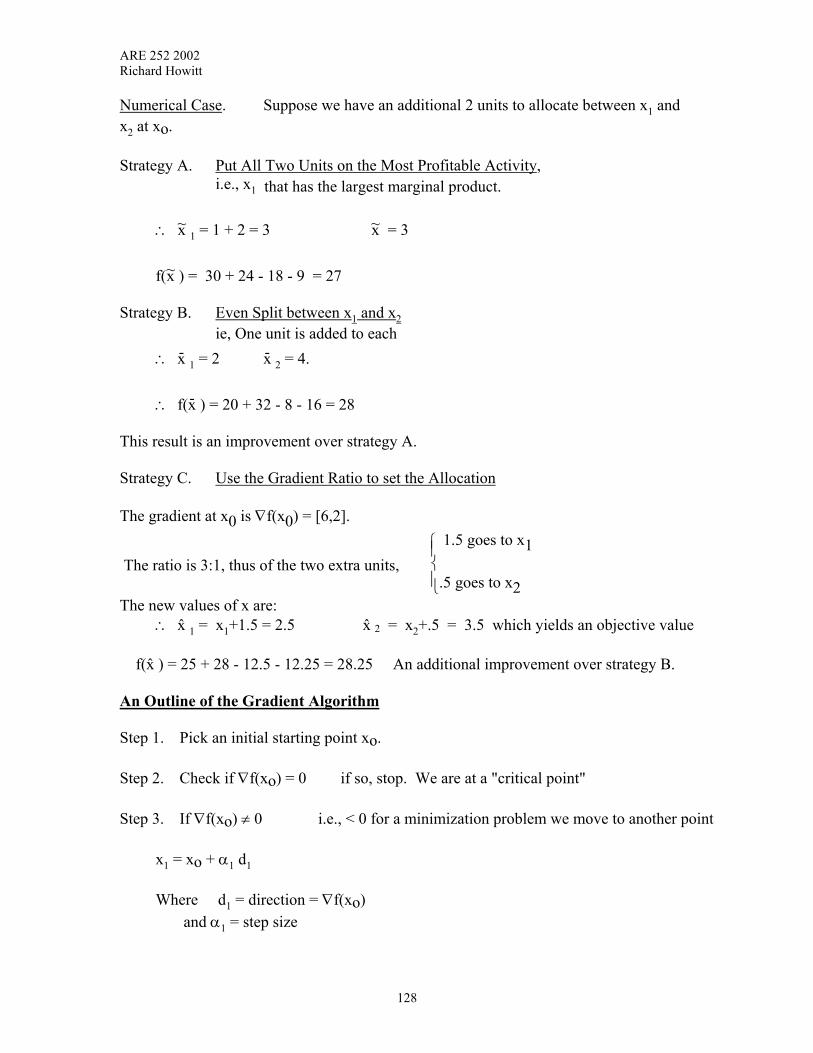
ARE 252 2002 Richard Howitt
Numerical Case. Suppose we have an additional 2 units to allocate between x1 and x2 at xo. Strategy A. Put All Two Units on the Most Profitable Activity, i.e., x1 that has the largest marginal product. ∴ x~ 1 = 1 + 2 = 3 x~ = 3 f(x~ ) = 30 + 24 - 18 - 9 = 27 Strategy B. Even Split between x1 and x2 ie, One unit is added to each ∴ x- 1 = 2 x- 2 = 4. ∴ f(x- ) = 20 + 32 - 8 - 16 = 28 This result is an improvement over strategy A. Strategy C. Use the Gradient Ratio to set the Allocation The gradient at x0 is ∇f(x0) = [6,2].
The ratio is 3:1, thus of the two extra units, 1.5 goes to x1 .5 goes to x2
The new values of x are: ∴ x 1 = x1+1.5 = 2.5 x 2 = x2+.5 = 3.5 which yields an objective value f(x ) = 25 + 28 - 12.5 - 12.25 = 28.25 An additional improvement over strategy B. An Outline of the Gradient Algorithm Step 1. Pick an initial starting point xo. Step 2. Check if ∇f(xo) = 0 if so, stop. We are at a "critical point" Step 3. If ∇f(xo) ≠ 0 i.e., < 0 for a minimization problem we move to another point x1 = xo + α1 d1
Where d1 = direction = ∇f(xo) and α1 = step size
128

ARE 252 2002 Richard Howitt
The objective function improvement condition f(xo + α1 d1) < f(xo) holds if and only if ⟨ ∇f(xo), d ⟩ < 0 for a minimization problem. Note (i) That this improvement condition is analogous to the negative rj criterion for entering activities in a minimizing LP problem (ii) The objective function improvement condition has the opposite sign to the first order optimality condition in equation (7) on page 77. This follows since the optimum is defined as the point where no improvement of the objective function is possible. Step 4. Return to Step 2. A two dimensional example
f(x)
α2
1α
x*
0xx1
f(x)
x
(1) Objective – Select x to minimize f(x) (2) Start at x0. ∇f(xo) = slope > 0, so choose d<0 to satisfy the objective function improvement condition ⟨∇f(xo),d⟩ < 0. (3) With stepsize α1 we arrive at x1. At x1 ∇f(x1)<0, so we choose d>0 to satisfy ⟨∇f(x1),d⟩ < 0. (4) With stepwise α2 we arrive at x*. Note, in this example I faked the selection of α1 and α2 . (5) At x*, ∇f(x*) = 0 and ⟨∇f(x*), d⟩ ≥ 0. Therefore we are at the minimum .
129

ARE 252 2002 Richard Howitt
Practical Problems with Gradient Algorithms 1. Starting points must be feasible. • Hint: linearize it crudely, find points in the feasible set, use them as starting point. • GAMS gives initial conditions that are feasible. 2. Step size • The stepsize must not take you out of feasible set at each iteration
α Here α is small and will require many iterations but it will work
α Here α is so big you miss the optimum A self-adjusting step size gets smaller as it moves in towards the optimum.
GAMS/MINOS defaults to this system. 3. Scaling Scaling the values of the data to balance the Hessian matrix of the objective function is a very important operation for all nonlinear solver routines. Th essential aspect is to scale the data values and the corresponding coefficients so that the eigenvalues of the Hessian are within three orders of magnitude of each other. Technically, the "condition value " for any matrix is the ration of the largest and smallest eigenvalue. An example is the best way of showing this. A very simple unconstrained quadratic problem can be defined as:
[ ] [ ] 11 121 2
21 22
X XZ X Y
Y Yγ γ
α αγ γ
= −
130

ARE 252 2002 Richard Howitt
In case 1 Well Scaled: α = [ 10.585, 2.717] and 0.3786 0.005780.00578 0.02193
Γ =
The eigenvalues for this matrix are 0.3787, 0.0218, the condition number is therefore 17.37. The surface to be searched by the algorithm appears as follows: Note that the surface gradients with respect to X and Y are quite similar and the calculation of a gradient will have a similar rounding error in each direction.
131

ARE 252 2002 Richard Howitt
Case 2 Badly Scaled: α = [ 10.585, 0.2717] and 0.3786 0.005780.00578 0.000219
Γ =
The eigenvalues for this matrix are 0.3787, 0.0001, the condition number is
therefore 3787. Note that a scaling of 10 on variable Y has increased the condition number 218 times. The surface to be searched by the algorithm appears is now:
Note that the gradients are very different and the Y axis values are multiplied by 10. The same rounding errors and step size are applied in both directions, but have very different effects on the change in the objective Z value. Thus the gradient will try and converge in one dimension but not the other. This "poorly scaled" condition creates a "hill" on the objective function surface that is very narrow, and the algorithm may "fall off" the surface. Given that the rounding error
132

ARE 252 2002 Richard Howitt
in calculating the numerical gradients is the same for the very large and small values the proportional error will be magnified by large differences in scaling. Reduced Gradients For constrained nonlinear optimization problems it is very common for the number of nonzero activities in the optimal solution to be greater than the number of binding constraints. Thus, there may be m binding constraints and k (k ≥ m) activities in the optimum solution, as in the case where we could use the PMP approach. However, all k activities enter the constraint set despite the m dimensional basis. The reduced gradient is the nonlinear analog to the reduced cost in L.P., and incorporates the linkages between activities due to the constraints. The net effect of a marginal change must therefore consider the direct gradient and the effect on other gradients, due to the linkage of the constraints. Given the constrained nonlinear problem
Min f(x)
Subject to A x ≥ b x ≥ 0 and qx1
At any point, the qx1 vector x can be partitioned into three sets. xB a m x 1 set of basis (dependent) variables xN a k x 1 set of independent variables x0 a (q–m–k) x 1 set of zero valued variables. Likewise, the matrix A can be partitioned into three matrices B, mxm basis matrix, N an mxk matrix of technical coefficients for the independent variables and D, an m x (q–k–m) matrix for the zero valued variables. Without loss of generality we can drop the zero valued variables (x0) and the nonbinding constraints from the problem. The problem becomes
Min f(xB,xN)
Subject to BxB + NxN = b
Using the constraint, the dependent variables can be written as a function of the independent variables.
133

ARE 252 2002 Richard Howitt
xB = B–1b – B–1NxN
Substituting this expression back into the objective function produces two useful characteristics. (1) The effect of the binding constraints are incorporated in the objective function. (2) The whole problem is expressed as a function of only the independent variables ( xN ).
Min f(B–1b–B–1NxN , xN)
The resulting "Reduced Gradient" for this problem is:
rxN = ∇fxN
(⋅) – ∇fxB (⋅) B–1N
The reduced gradient captures the net effect of a marginal change in an independent variable. Necessary Condition It can be shown (Luenberger) that a necessary condition for a linearly constrained nonlinear optimization is that all the reduced gradients are zero. Note. The GAMS/MINOS algorithm uses reduced gradients for this purpose and prints the "rg" value on the right hand side of the activities for nonlinear problems.
Newton's Method Newton's Method uses the Hessian as well as the gradient to search over the set of all the critical stationary points, i.e., where ∇f(x) = 0. Since we now consider a sequence of algorithm steps, we use the more general notation of k, k+1, k+2, etc. Derivation: 1. Starting at some point xk , we wish to move to a new point x k+1, which has the
property that it is a critical point
∇f(xk+1 )′ = 0 In this method we start with the gradient and expand around it. 2. Using a Taylor Series expansion of the gradient around xk (first-order)
134

ARE 252 2002 Richard Howitt
∇f(xk+1 )′ ≈ ∇f(xk )′ + Hxk (xk+1 - xk)
set= 0 where Hxk
is the Hessian of f(x) at xk . From step (2) we see that the stationary point condition ∇f(x
k+1 ) = 0 implies that:
3. Hxk
(xk+1 - xk ) = -∇f(xk)′ Multiply (3) by H-1
xk (assuming that the Hessian is nonsingular and invertible) and
move xk to the right hand side to yield:
xk+1 – xk = – H ∇f(x x-1
k k)′
∴ xk+1 = xk - H-1xk ∇f(xk)′
Note: With a quadratic objective function, a stationary point xk+1 is reached in one
step! An example of Newton’s (1642 - 1727) mind at work ,which is still topical after three hundred years. Beautiful!
Example: Newton’s Method applied to a Quadratic Problem
f(x) = a'x + 1/2 x'Bx where the hessian matrix B is nonsingular and positive definite at xo. Taking the gradient ∇f(xo)′ = (a + Bxo)′ Hxo = B (Note, this is independent of choice of xo) ∴ Apply Newton's Method x1 = xo - B-1(a+Bxo) = -B-1a (Also independent of choice of xo). Check. Is x1 a stationary point?
Plug in ∇f(x1)′ = a + Bx1 Substitute the Newton value for x1 above. = a + B(-B-1a)
135

ARE 252 2002 Richard Howitt
= a-a = 0. ∴ We have reached a stationary point in one step. Note: For nonquadratic functions, the Newton is an approximation to the function and therefore will take several steps. However, if the Hessian is "well conditioned," Newton's method will converge rapidly. Caveats on Newton's Method 1. The Newton approach finds stationary points, it does not guarantee that they're
global or even local optima. 2. The Hessian is often hard to invert.
Criteria for Non-Linear Algorithms
1. Theoretical convergence rate Newton is faster than the steepest decent method 2. Computational difficulty Newton requires generating, then inverting the Hessian 3. Numerical stability Newton requires well-conditioned Hessians
Newton Stepsize: Used when the objective function is not quadratic in form. In this case the Taylor expansion that forms the basis of the Newton derivation is only an approximation of the function. xk+1 = xk – αH-1
xk ∇f(xk)′ for a minimization problem. Note: If Hxk is an identity matrix, then this is equivalent to the steepest descent method and reduces to: xk+1 = xk–α∇f(xk)′ Necessary conditions for movement towards a minimum with the Newton method are clarified by a change to condensed notation. Define the notation: dk = –H-1
xk ∇f(xk)′ = direction
136

ARE 252 2002 Richard Howitt
137
Mk = H-1xk for simplicity of algebra
gk = ∇f(xk)′ for simplicity of algebra For minimum: We require the "downhill" condition in the new notation to be, ⟨dk, gk⟩ < 0 i.e., dk′gk<0 Using the notation defined above this is equivalent to: (–Mkgk)′gk < 0 or gk′Mkgk > 0
This is most easily fulfilled if Mk = H-1xk is a positive definite matrix.
Desired Conditions for Hxk 1. Non-singular 2. Positive definite 3. Well-conditioned (eigenvalues within 103 of each other) How to make an Ill-conditioned Hessian Well-conditioned: 1. Greenstadt's Method - Similar to ridge regression
2. Scaling - a much better approach that aims to change the units of measurement associated with the Hessian so they are "close" i.e., within (103) of each other.
The Gams solver Conopt2 now has an effective scaling routine that updates the scaling factors as the solver progresses. This scaling option should not be confused with the standard Gams scaling option that scales the Gams problem before the solver is called. The Conopt2 scaling system has to be called from an appropriate “Options “ file in the Gams program. For an example of a Conopt2 options file see chapter 10.
For a more extensive discussion on scaling see: Gill, Murray, and M. Wright, "Practical Optimization," Academic Press, pp. 346-354.


