Optimization of a Vanadium Redox Flow Battery with...

IN DEGREE PROJECT ELECTRICAL ENGINEERING, SECOND CYCLE, 30 CREDITS

, STOCKHOLM SWEDEN 2016

Optimization of a Vanadium Redox Flow Battery with Hydrogen generation

DANIEL WRANG

KTH ROYAL INSTITUTE OF TECHNOLOGYSCHOOL OF ELECTRICAL ENGINEERING

AcknowledgementsI would like to thank my supervisor Dr. Timm Faulwasser and co supervisor Dr. Julien

Billeter at EPFL for inviting me to work with them and for their input and support during

the development of this thesis. I would also like to express my gratitude to Prof. Dominique

Bonvin, EPFL, for hosting me at the Laboratoire d’Automatique at EPFL. I would like to

thank Dr. Véronique Amstutz, Dr. Alberto Batisel and Dr. Heron Vrubel, at EPFL for helping

with development of the electrochemical aspects of the battery model. I am thankful to my

examiner Prof. Mikeal Johansson, KTH.

i

AbstractWe consider the modelling and optimal control of energy storage systems, in this study a

Vanadium Redox Flow Battery. Such a battery can be introduced in the electrical grid to be

charged when demand is low and discharged when demand is high, increasing the overall

efficiency of the network while reducing costs and emission of greenhouse gases. The model

of the battery proposed in this study is less complex than the majority of models on batteries

and energy storage systems found in literature, but still accurate enough to capture the core

aspects of the behaviour of the battery. Estimation methods are discussed for determining

unknown parameters in the model using experimental data and the model is evaluated against

additional measurements of the physical system showing good fit. The purpose of having a

simple model is that the resulting optimal control problem is easier to solve. Operation of the

battery with respect to several different objectives are discussed and that of minimizing the

vertical net load and maximizing profit are solved for open loop control and receding horizon

control over the time span of one day. Two performance metrics are proposed for determining

the gain of operating an electrical network with or without the battery. The results show that

the introduction of storage systems indeed helps in increasing profit and reducing emissions.

iii

ContentsAcknowledgements i

Abstract iii

1 Introduction 1

1.1 Motivation . . . . . . . . . . . . . . . . . . . . . . . . . . . . . . . . . . . . . . . . . 1

1.2 Literature survey . . . . . . . . . . . . . . . . . . . . . . . . . . . . . . . . . . . . . 4

1.3 Problem definition . . . . . . . . . . . . . . . . . . . . . . . . . . . . . . . . . . . . 6

2 Preliminaries 7

2.1 Experimental setup . . . . . . . . . . . . . . . . . . . . . . . . . . . . . . . . . . . . 7

2.2 Differential algebraic equations . . . . . . . . . . . . . . . . . . . . . . . . . . . . 9

2.3 Optimal control . . . . . . . . . . . . . . . . . . . . . . . . . . . . . . . . . . . . . . 10

3 Modeling 13

3.1 Battery properties . . . . . . . . . . . . . . . . . . . . . . . . . . . . . . . . . . . . . 13

3.2 Battery model . . . . . . . . . . . . . . . . . . . . . . . . . . . . . . . . . . . . . . . 14

3.3 Full model . . . . . . . . . . . . . . . . . . . . . . . . . . . . . . . . . . . . . . . . . 18

3.4 Discussion . . . . . . . . . . . . . . . . . . . . . . . . . . . . . . . . . . . . . . . . . 19

3.5 Electrolysis . . . . . . . . . . . . . . . . . . . . . . . . . . . . . . . . . . . . . . . . . 19

3.6 Parameters . . . . . . . . . . . . . . . . . . . . . . . . . . . . . . . . . . . . . . . . . 20

4 Parameter estimation and validation 23

4.1 Methods . . . . . . . . . . . . . . . . . . . . . . . . . . . . . . . . . . . . . . . . . . 23

4.2 Results . . . . . . . . . . . . . . . . . . . . . . . . . . . . . . . . . . . . . . . . . . . 26

4.3 Model validation . . . . . . . . . . . . . . . . . . . . . . . . . . . . . . . . . . . . . 29

5 Optimization 33

5.1 The electrical network . . . . . . . . . . . . . . . . . . . . . . . . . . . . . . . . . . 33

5.2 Constraints . . . . . . . . . . . . . . . . . . . . . . . . . . . . . . . . . . . . . . . . . 35

5.3 Objective function . . . . . . . . . . . . . . . . . . . . . . . . . . . . . . . . . . . . 36

5.4 Optimal control problem . . . . . . . . . . . . . . . . . . . . . . . . . . . . . . . . 40

5.5 Implementation aspects . . . . . . . . . . . . . . . . . . . . . . . . . . . . . . . . . 41

5.6 Performance metrics . . . . . . . . . . . . . . . . . . . . . . . . . . . . . . . . . . . 41

v

Contents

6 Results 45

6.1 Data . . . . . . . . . . . . . . . . . . . . . . . . . . . . . . . . . . . . . . . . . . . . . 45

6.2 Open loop optimization over one day . . . . . . . . . . . . . . . . . . . . . . . . . 48

6.3 Receding horizon optimization over one day . . . . . . . . . . . . . . . . . . . . . 51

7 Conclusions and future work 55

7.1 Conclusions . . . . . . . . . . . . . . . . . . . . . . . . . . . . . . . . . . . . . . . . 55

7.2 Future work . . . . . . . . . . . . . . . . . . . . . . . . . . . . . . . . . . . . . . . . 55

A Derivation of the battery model 57

B Additional validation results 65

B.1 Estimation results . . . . . . . . . . . . . . . . . . . . . . . . . . . . . . . . . . . . . 65

B.2 Validation results 1 . . . . . . . . . . . . . . . . . . . . . . . . . . . . . . . . . . . . 68

B.3 Validation results 2 . . . . . . . . . . . . . . . . . . . . . . . . . . . . . . . . . . . . 71

C Additional optimization results 77

C.1 Receding horizon over one week . . . . . . . . . . . . . . . . . . . . . . . . . . . . 77

Bibliography 83

vi

1 Introduction

1.1 Motivation

Renewable means of electricity production are among others photovoltaics (solar panels),

wind turbines and hydroelectric plants. Hydroelectric power has advantages as the water can

be stored and used upon request, but most regions do not meet the geographical requirements

for construction. Photovoltaics and wind turbines can be built in most areas but have the

disadvantage that the electrcity production is intermittent and strongly depends on external

factors. In general, in order to keep the electric grid working it is required that production and

consumption are in balance which means that electricity has to be produced when consumed.

A problem emerges if there is too much or too little electricity produced. This issue can be

overcome by introducing large scale energy storage systems so that the excess electricity

produced at low demand periods can be stored and later be used during high demand periods.

The introduction of energy storage systems opens up for a more dynamic electrical grid where

consumers and producers will be able to increase the energy efficiency and emissions can

be reduced. This project aims at suggesting how such a storage system can be modelled and

incorporated in the electrical network and furthermore, how the battery should be operated to

maximize its performance. For this study, the storage system consisted of a Vanadium Redox

Flow Battery (VRFB), additionally, in the experimental setup there is also an electrolyser for

storage in form of hydrogen gas which increases the capacity. The setup is illustrated in Figure

1.1.

Energy storage systems

There exists numerous alternatives to the VRFB for storing energy, see e.g. [1] for an overview

of various other options for energy storage. The most widespread ones may be classified into

mechanical, electrical and electrochemical storage systems. Mechanical systems include for

instance flywheels, pumped hydro systems and compressed air energy storage. Electrical

systems include supercapacitors and superconducting magnetic energy devices. Electro-

chemical systems include batteries of different types, those with solid compounds and redox

1

Chapter 1. Introduction

flow batteries such as the one in this study. Some advantages of the VRFB over other storage

systems are, 1) the VRFB does not contain any toxic substances, 2) the VRFB contains the same

chemical substance, vanadium in both electrolytes which means that cross mixing of species

through the membrane is not a problem [1, 2] and 3) storage capacity and delivered power

are independent in the VRFB. By increasing the size of the tanks will the storage capacity

be increased and by increasing the number of stacks will the delivered power capacity of

the battery be increased. The advantage is that these two properties of the battery can be

increased independently either to optimize the battery for a specific storage size or for high

power supply. The VRFB is typically too large for one household, but can be built small enough

to be suitable for remote areas or small communities.

2

1.1. Motivation

Figure 1.1 – A network of a small energy grid.

3


1.2 Literature survey

In this part, some previous studies of the modeling of batteries and other energy storage

systems and control strategies and optimization of such systems are briefly discussed.

Battery modelling

A thorough model of the VRFB based on principles from electrochemistry but also elements of

fluid dynamics when modelling the flow of liquids in the tanks is described in [1]. Various con-

figurations of tank size and number of cells in the battery are also considered. Another paper

[3] investigates modelling of a VRFB from electro chemical and fluid mechanics principles

resulting in a more complex model than the one presented in this thesis. The model is also

compared with measurements of real systems demonstrating a good fit of the model.

In another paper ideas for modeling redox flow batteries and other large scale battery systems

using an equivalent electric circuit model are presented [4]. Using this approach, resistors may

represent losses and resistance due to chemical reactions occurring in the battery. Voltage or

current sources may serve as control signal. This paper particularly focuses on the vanadium

redox flow battery and takes chemical aspects of the system into account in the model.

Control of electrolyte flow

In the VRFB under study in this thesis the pumps are not directly controlled. However, the

liquid flow rate may be optimized to increase battery performance. In [5] the flowrate was

investigated. They studied how to vary the flowrate to increase the overall system efficiency.

In [6] a strategy for optimizing the liquid flow of a vanadium redox flow battery (VRFB) is

presented. The authors performed experiments on a small scale VRFB by varying the flow rate

and measuring the response of the system; using these data they could compute efficiency of

the battery and determine the optimal flowrate for charge and discharge respectively. Their

results show that an increase in efficiency of 8% is achievable if using the optimal flowrate

compared with the worst case.

Optimization of energy storage systems

In the literature there exists various studies of optimal control polices for different types of

Energy Storage Systems (ESS), where the term ESS is used in a broader sense than redox flow

batteries. In [7], the authors consider a storage system connected to a wind farm. A simple

model of the battery is proposed, an electric circuit analogy is used for modelling the dynamics

of the battery.

In [8], the authors describe a system setup that tries to minimize costs in a network with

fluctuating prices by providing an optimal scheme for when to charge and discharge the

4

1.2. Literature survey

storage system. Some residential houses are considered and act as customers of energy, these

customers also produce electricity themselves via solar panels on their houses.

[9] considers energy storage systems as an complement to diesel generators for remote lo-

cations that normally are supplied by renewable energy sources such as windpower. By

introducing a storage system to keep the surplus energy from renewable sources to store

excess, if any from the windpower plant, the amount of diesel required can be reduced.

In one paper an energy storage system connected to the grid and charged using wind power

is discussed [10]. No model or dynamic equations are derived, instead only the power from

the wind power and to the battery and grid are considered. The authors aim at minimizing

fluctuations from some predefined levels of how much of the energy to distribute to the battery

and how much to the grid. The optimization formulation results in a quadratic cost function

with linear constraints and the idea is to compute the open loop control for the following day

using wind prediction data.

Modeling and optimization of energy storage systems

Several authors considered the modeling and optimization of energy storage systems. Vossen

et al. [11] investigated modelling and optimal control for a lithium-ion battery cell. They

studied time optimal charging but also took battery aging into account by always keeping the

battery temperature strictly below a certain limit. The solution results in a bang-bang control

under normal conditions, but the control signal becomes limited when the temperature of

the battery reaches the threshold that hastens aging. When the temperature threshold is

reached the control is determined such that the temperature is maintained at the threshold.

The authors do not consider the battery connected to the grid.

One study [12] discussed a simple setup of arrays of solar panels and a battery system for

electricity storage. The authors then discuss several objectives of operating the battery and

formulates the corresponding objective functions for the optimization problems. They con-

sider maximization of the state of charge level of the battery, preventing aging of battery,

maximizing the self consumption of the battery and maximizing profit of operating the battery

when connected to the main grid. A higher temperature or higher state of charge causes the

battery to age faster according to the authors. Maximizing the self consumption, which can

be found in the literature does in this case refer to using as much of the energy stored in the

battery as possible and selling as little as possible to the main grid and should not be confused

with self consumption of the battery where the state of charge decays after time if the battery

is not used.

In [13], a more general battery energy storage system is studied and modeled using a simplified

electric circuit model. The battery system is connected to the grid and charged using energy

from wind plants. An optimal control problem aiming at following a reference power is

proposed and solved using model predictive control subject to physical constraints on the

5


system and dynamic equations of the system.

1.3 Problem definition

The dynamics of the VRFB is modeled, a model of the VRFB suitable for control purposes

without to much details about the underlying chemistry is considered. Next estimation of pa-

rameters in the model is conducted using experimental data and the model is validated using

additional data. Finally optimal control strategies for different production- and consumption-

scenarios are investigated. To the best of our knowledge, no one has before considered optimal

control policies of such a battery in combination with a simple model of the VRFB proposed

in the study.

6

2 Preliminaries

2.1 Experimental setup

The experimental platform consists of a Vanadium Redox Flow Battery coupled with an elec-

trolyser for hydrogen generation, this setup is described in more detail in [2]. An electrolyser

is a device for splitting molecules into its ions, in this case water into hydrogen and oxygen.

Basics of the Vanadium Redox Flow Battery

An in depth study of the VRFB is presented in [1]. A brief description of the battery is presented

here based on those findings. A reader unfamiliar with flow batteries or electrochemistry is

recommended to take a look at [16], which contains a brief introduction to the VRFB including

a short informative video. The VRFB is a flow battery which stores energy in two tanks. One

tank contains the V (IV )/V (V ) species and the other the V (I I )/V (I I I ) species. In a flow

battery, energy is stored in electrolytes in liquid form as opposed to other batteries which

contain solid substances. The tanks are connected through pipes to a series of cell stacks.

In the VRFB under study there are 120 cells assembled in 3 parallel strings composed of two

stacks containing 20 cells each, so in essence 3 parallel stacks of 40 cells in each stack. The

liquids are pumped through the pipes and chemical reactions in the cells giving rise to a

flow of electrons when a current or a potential is applied. The liquid flow are controlled by

pumps and may be adjusted independently of the electrical load of the system, however,

controlling the pumps was not investigated in this thesis. Pump speed and thus the electrolyte

flowrate was controlled by a low level control system to prevent damage on the battery. The

cells are connected with electrical wires so that current may be taken from or supplied to the

cells. The direction of the current in the cells determine the chemical reaction occurring and

consequently if the battery is being charged or discharged. In each cell stack there is an ion

exchange membrane separating the V (I I )/V (I I I ) species from the V (IV )/V (V ) species. The

membrane allows for single protons H+ to be transferred between the solutions to maintain

charge balance, since electrons are extracted. The VRFB is schematically illustrated in Figure

2.1.

7

Chapter 2. Preliminaries

Figure 2.1 – A schematic view of the VRFB with one cell [17].

The following reactions occur in the cells of the VRFB

At the negative electrode (cathode) V (I I )/V (I I I )

V (I I I )+e− →V (I I ) charge (2.1)

V (I I ) →V (I I I )+e− discharge (2.2)

At the positive electrode (anode) V (IV )/V (V )

V (IV )+H2O →V (V )+2H++e− charge (2.3)

V (V )+2H++e− →V (IV )+H2O discharge (2.4)

where V is the element Vanadium and the notation V (I I I ) is used instead of V 3+ and V (I I )

is used instead of V 2+ and similarly the notation V (IV ) is used instead of V O2+ and V (V )

is used instead of V O+2 , thus there is balance in the oxygen O and hydrogen H in the above

chemical reactions. The free electrons present in the chemical reactions are those that are

transfered from or to the electrolytes and that give rise to current over the battery.

8

2.2. Differential algebraic equations

Electrolyser

An electrolyser is a device for forming hydrogen gas, H2 from water using electricity, the

chemical overall reaction is

2H2O → 2H2 +O2

where oxygen O2 is a rest product and energy is required for the reaction to occur. The

hydrogen gas may then be stored and burned with oxygen to again form water molecules,

when the reversed chemical reaction takes place; hydrogen gas is therefore a zero emission

fuel. The purpose of introducing electrolysis is to make use of excess energy when the battery

is fully charged. The produced hydrogen gas could be converted back into power, however, in

this setup it is assumed that the hydrogen is sold instead.

2.2 Differential algebraic equations

Some basic results on Differential Algebraic Equations (DAEs) of relevance for this study are

presented here. We assume the initial conditions x(t0) = x0 and z(t0) = z0 are known. Through-

out this thesis only autonomous systems are considered, i.e. there is explicit t dependence.

We consider a general DAE on the form

F (x, x, z,u) = 0 (2.5)

with output

y = h(x, z,u) (2.6)

thus the states x and z may not be measurable, instead y is measurable, with x the differential

states, x the derivative of the differential states with respect to time, z the algebraic states and

u the manipulated variable. If the DAE can be written as

E x =G(x, z,u) (2.7)

where the mass matrix E is singular and an appropriate function G , the DAE is said to be semi

explicit. This can be rewritten

x = f (x, z,u) (2.8)

0 = g (x, z,u) (2.9)

where dim( f ) = dim(x) and dim(g ) = dim(z). An important property of DAE systems is its

index [18]. The index of the DAE is defined as the number of times one must differentiate the

9

Chapter 2. Preliminaries

entire DAE with respect to time t in order to obtain an ODE system on the form

x = f (x, z,u) (2.10)

z = gd (x, z,u) (2.11)

where gd is the function obtained after differentiation that allows us to write the system as

an Ordinary Differential Equation (ODE). Many numerical DAE solvers require the system

to be index 1 and if that is not fulfilled the index of the system needs to be reduced. Index

reduction was not used in this study, but a good source on how to do index reduction is [18].

Index reduction may also be done using numerical software, e.g. MATLAB or Mathematica.

For a semi explicit system the algebraic constraints of the DAE are expressed by (2.9), then, if

the Jacobian matrix, J = ∂g (x,z)∂z is full rank or equivalently, det(J ) 6= 0 then the system (2.8)-(2.9)

has differential index 1 and can be solved directly using numerical software, without index

reduction or reformulation of the system [18].

DAE solvers

Broadly, two different approaches for solving DAE systems exist. The discussion is limited

to semi explicit DAEs as only such DAE systems were studied. For a more general overview

the reader can refer to [18]. Consider a semi explicit DAE, with x = f (x, z) and 0 = g (x, z). In a

direct method g (x, z) = 0 is first solved for z using a nonlinear equation solver then x = f (x, z)

is solved as an ODE. Another method is based on Backward Differentiation Formula (BDF)

integrators [18]. This is an implicit integration method particularly well suited for stiff ODE

systems and for handling DAEs [18], the Backward Euler method is an example of a BDF

integrator [18].

2.3 Optimal control

Some fundamental results on optimal control are presented in this chapter, to be used when

formulating the optimal control problem of the VRFB.

The optimization problem to be solved is stated as

minimizex(·),z(·),u(·)

M(t f , x f , z f )+∫ t f

t0

L(t , x, z,u)d t

subject to F (t , x, x, z,u) = 0

gi (t , x, z,u) ≤ 0

h0(t0, x0, z0) = 0

h f (t f , x f , z f ) = 0

(2.12)

with x the dynamical variables and z the algebraic variables and where t0 is the initial time,

t f is the final time, x0 = x(t0), z0 = z(t0), x f = x(t f ) and z f = z(t f ). The function F (·) = 0 de-

10

2.3. Optimal control

scribes the DAE, gi (t , x, z,u) are the inequality constraints that must be satisfied, h0(t0, x0, z0)

describes the starting conditions of the system if such constraints exist and h f (t f , x f , z f )

describes the conditions that must be fulfilled at the final time if such constraints exist. The

function M(t f , x f , z f ) is the terminal cost, in the literature referred to as a Mayer term and

L(t , x, z,u) is the cost at each time throughout the interval, in the literature referred to as a

Lagrange term.

Solving optimal control problems

An Optimal Control Problems (OCP) is normally very hard to solve analytically, therefore

various numerical methods have been developed for solving optimal control problems. In

[19] an introduction to computational methods for optimal control is presented and methods

such as direct discretization, single and multiple shooting and consistent approximation are

discussed. To facilitate the usage of these numerical algorithms for optimal control much

effort has been put in developing toolboxes for solving an OCP. One such toolbox is GPOPS II

[20], that can be used for solving general optimal control problems.

11

3 Modeling

3.1 Battery properties

The battery has a nominal capacity of 40 kWh, can deliver a nominal power of 10 kW and a

maximum power of 15 kW [21]. The battery installed in Martigny has an internal low level

control system that could not be bypassed and sometimes may affect the behavior of the

battery by suddenly causing power, voltage or current levels to change.

State of charge

The State Of Charge (SOC) of the battery can be interpreted as a fuel meter of the battery. The

VRFB under study has two tanks, each with a capacity of 1000 L [21] and the concentration

of the electrochemically active species in these tanks determine the SOC. The SOC will be

measured in %, and thus ranges between 0 and 100. A relation for the SOC commonly used in

the literature and independent of the energy storage system is described in [22], which here

has been multiplied by 100 to be in (%), is

x(t ) = x(t0)+∫ t

t0

100ηC

CNi (τ)dτ (3.1)

where x(t) is the SOC (%) and i (t) is the current (A). The parameter ηC is the Coulombic

efficiency (-), i.e. how much of the charge that is put into the battery can be returned, ηC ∈ [0,1].

The parameter CN is the nominal (or total) capacity of the battery (C). The state of charge may

be formulated

x(t ) = 100ηC

CNi (t ), x(t0) = x0 (3.2)

and this differential equation will be part of the model of the VRFB.

13

Chapter 3. Modeling

Battery current

Due to the chemical reactions described previously that occur inside the cells of the battery,

electrons are transfered that give rise to a current in the battery. Internally, the battery has 6

stacks assembled in 3 parallel lines and the total current of the battery is the sum of the current

over the 3 lines. Each line is composed of two stacks in series, each of them comprising 20

cells in series. For simplicity it will be assumed that the current of all stacks is the same.

Battery voltage

Each cell has two electrodes and the difference of potential between the electrode and vana-

dium solution in each half cell are internal states of the system and will be included in the

model. However, these states cannot be observed. For modeling purposes it will be assumed

that all of the 120 cells have the same electrode potentials. The total DC voltage of the battery

can be measured and is limited to the interval [42, 63] (V) to prevent damages to the battery.

Battery power

The power of the battery is the control signal and thus the decision variable in the optimization

problem on how to operate the battery. The battery will normally be operated around the

nominal power level (10 kW). The power on the grid is in alternating current (AC), whereas the

power inside the battery is in direct current (DC). Thus between the battery and the grid there

are DC/AC/DC converters and in the conversion there are energy losses. The efficiency of the

DC/AC/DC conversion needs to be taken into account.

The relation in a DC system between the power P (W), current I (A) and voltage U (V) is given

by

P =U I (3.3)

When modeling the battery, the sign convention will state that the current is positive when the

battery is charging and negative when discharging. Note that this convention concurs with the

equation relating current to SOC (equation 3.2), since the efficiency and capacity are positive.

3.2 Battery model

The models of batteries found in the literature based on electrochemical and fluid mechanics

principles are quite complex and for the purpose of this thesis a simple model that captures

the core aspects of the battery will be used [1].

Let x denote the state of charge of the battery which is a dynamic variable, the state of charge

will be measured in % and thus ranges in the interval [0, 100]. Next let z = (z1, z2, z3, z4) be

the vector of algebraic variables, where z1 is the battery current (A), z2 is the potential at the

14

3.2. Battery model

V (I I I )/V (I I ) electrode (V), z3 is the potential at the V (IV )/V (V ) electrode (V) and z4 is the

power of the battery (W).

Model of a single cell

Using the two algebraic relations linking the current and the electrode potentials (A.31)-(A.32),

the relation between power, current and voltage (3.3) and the differential equation for the

state of charge (3.2), the dynamics of the VRFB with one cell can be written as the Differential

Algebraic Equation (DAE) (3.4)-(3.7)

x = k0 · icel l (3.4)

0 = icel l −z4

Eapp,cel l (x, z)(3.5)

0 =−icel l −k6(x)

(exp

(k2α2(x, z2)

)−exp(k3α2(x, z2)

))(3.6)

0 = icel l −k7(x)

(exp

(k4α3(x, z3)


))(3.7)

where icel l is the current in the single cell (A). This is completed by the following relations that

are also derived in the appendix

s(x) = 1−0.01x

0.01x(3.8)

a(x) = (2+0.01x ·k10)2

s(x)(3.9)

Eapp,cel l (x, z) = z2 + z3 −2 ·k8 −k1 ln[s(x)3a(x)] (3.10)

and

α2(x, z2) = z2 −(k8 +k1 ln[s(x)]

)(3.11)

α3(x, z3) = z3 −(k9 +k1 ln[a(x)]

)(3.12)

and

k6(x) = i0,32 · c3(x)α32 c2(x)(1−α32)F (3.13)

k7(x) = i0,54 · c5(x)α54 c4(x)(1−α54)F (3.14)

where F is the Faraday constant, x is the SOC in the interval [0, 100] and

c2(x) = x ·k10

100(3.15)

c3(x) = k10 − c2(x) (3.16)

15

Chapter 3. Modeling

and similarly

c5(x) = x ·k10

100(3.17)

c4(x) = k10 − c5(x) (3.18)

where c2(x), c3(x), c4(x) and c5(x) are the concentrations of the respective vanadium species.

Model of the complete battery

Due to the cells and stack arrangement the current of the battery is

z1 = ibat ter y = 3 · icel l

and the voltage as

Eapp (x, z) = 40 ·Eapp,cel l (x, z)

The power of the battery is

z4 = z1 ·Eapp (x, z)

From these additional equations the DAE for the entire battery becomes (3.19)-(3.22)

x = k0 · z1 (3.19)

0 = z1 − z4

Eapp (x, z)(3.20)

0 =−z1 −3 ·k6(x)

(exp

(k2α2(x, z2)


))(3.21)

0 = z1 −3 ·k7(x)

(exp

(k4α3(x, z3)


))(3.22)

with the same notation as previously. The system needs to be solved for the variables

(x, z1, z2, z3, z4). However, there are only four equations, but by considering the battery in

either constant power or in constant voltage mode, one more algebraic equation is introduced.

Power driven mode

During constant power mode, the DAE can be complemented by

0 = u − z4 (3.23)

where u is the manipulated variable. However, if the system reaches one of the battery

threshold voltages the battery switches to constant voltage mode. During normal operation

16

3.2. Battery model

the battery will be operated in constant power mode.

Constant voltage mode

During the charge the voltage in the battery increases until the voltage level hits a threshold of

63 (V) when the battery switches to constant voltage mode. Similarly, during the discharge the

voltage decreases until the voltage reaches a threshold of 42 (V) when the battery switches

to constant voltage mode. Let Vconst be the constant voltage value, either 63 or 42, then the

following equation can be added to the DAE

0 =Vconst −Eapp (x, z) (3.24)

where Vconst is the upper or lower limit.

Parameters

To simplify and generalize the notation of the system model, the following parameters k0, . . . ,k5

and k8 . . .k10 are defined

k0 = 100ηC

CN

k1 = RT

F

k2 = α32n32

k1

k3 = −(1−α32)n32

k1

k4 = α54n54

k1

k5 = −(1−α54)n54

k1

k8 = E 0′32

k9 = E 0′54

k10 = aV tot

the meaning of the parameters on the right hand side of the equaltiy signs can be found at the

end of this chapter.

17

Chapter 3. Modeling

3.3 Full model

The model of the VRFB previously discussed is presented here in its full extent. It may be

expressed by equation (3.25) using equation (3.26)-(3.28), with F (x, x, z,u) = 0

F (x, x, z,u) =(

x − f (x, z,u)

g (x, z,u)

)(3.25)

where

f (x, z,u) = k0z1 (3.26)

g (x, z,u) =

z1 − z4

Eapp (x,z)

−z1 −3 ·k6(x)(exp(k2α2(x, z2))−exp

(k3α2(x, z2)))

z1 −3 ·k7(x)(exp(k4α3(x, z3))−exp

(k5α3(x, z3)))

g4(x, z,u)

(3.27)

with

g4(x, z) =u − z4 if constant power mode

Vconst −Eapp (x, z) if constant voltage mode(3.28)

Measurements of the system

The outputs of the VRFB that are measured are the state of charge, current, voltage and power

defined by

y = h(x, z,u) =

x

z1

Eapp (x, z)

z4

(3.29)

The electrode potentials z2 and z3 are typically not available as measurments. However, it is

physically possible to measure them, but it requires additional equipment. The VRFB can be

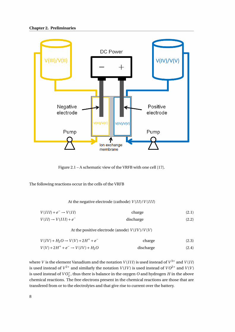
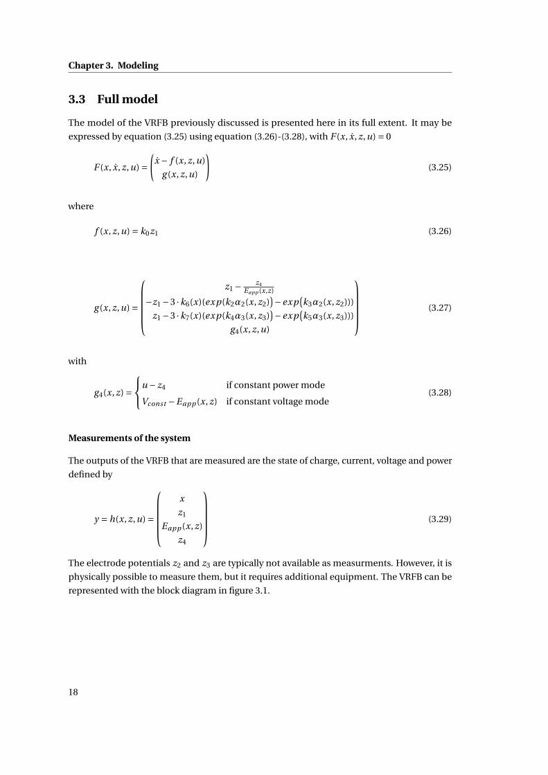
represented with the block diagram in figure 3.1.

18

3.4. Discussion

VRFBx = f(x, z, u)0 = g(x, z, u)y = h(x, z, u)

u y

Figure 3.1 – A block diagram of the VRFB with input and output.

3.4 Discussion

Why a DAE

All the measurable quantities in the model, voltage, current and power change over time.

However, since the dynamics of the current, voltage and power are much faster than that of

the state of charge, these quantities reach steady state values much faster than does the state

of charge. Therefore they are modelled as algebraic equations.

Existence of solution

The algebraic constraints of the DAE are expressed by equation (3.27), then, if the Jacobian

matrix, J = ∇g (x, z) is full rank or equivalently, det(J) 6= 0 then the system (3.26)-(3.27) has

differential index 1 and can be solved directly using numerical software, no index reduction or

reformulation of the system is necessary [18]. This was attempted but no analytic expression

of det(J ) 6= 0 simple enough to analyze could be obtained. However, det(J ) could be computed

numerically when simulating the system to determine the index of the system.

Other considerations

Self consumption of the battery has not been considered in the model, data [21] show that after

10 days the battery is completely depleted when it initially was fully charged and remained in

standby mode. Furthermore, voltage drop due to resistance in the wires at high currents has

not been modeled.

3.5 Electrolysis

In this study hydrogen storage is considered. The amount of energy stored in hydrogen is

modeled similarly as that of the state of charge for the battery. Define xH (t ) to be the amount

of energy stored in hydrogen (Ws) at time t and u2(t) being the amount of power (W) that

is used for hydrogen production, inspired by the relation for the state of charge, one simple

relation is

xH (t ) = xH (t0)+∫ t f

t0

αu2(τ)dτ (3.30)

19

Chapter 3. Modeling

from which we get the differential equation

xH (t ) =αu2(t ), xH (t0) is known (3.31)

whereα is a dimensionless efficiency factor, for this model it was set toα= 0.5. For the present

study we assume that the storage capacity of hydrogen is infinite, thus there is no restriction

on how much hydrogen can be stored.

3.6 Parameters

The parameters appearing in the model are presented. Some parameters are known from the

literature whereas others are dependent on the physical system and have to be determined

experimentally.

Constants

The values listed in Table 3.1 are physical constants related to the system that do not need to

be identified. They were either obtained from literature or from general information about the

particular battery under study.

Parameter Value Unit DescriptionR 8.314 J mol−1 K−1 Ideal gas constantT 298 K Absolute temperatureF 96485 C mol−1 Faraday constant

n32 1 - Number of electrons in half reaction for V (I I )/V (I I I )n54 1 - Number of electrons in half reaction for V (IV )/V (V )E 0′

32 -0.207 V Standard reduction potentialE 0′

54 1.18 V Standard reduction potentialaV tot 1.6 - Total activity

Table 3.1 – Constants.

R , T and F are standard physical constants found in the literature, n32 and n54 are the number

of electrons that are exchanged in each half reaction of the battery. It can be identified from

chemical equations (2.1)-(2.4). As can be seen, only one electron is taking part in each reaction

and therefore n32 = n54 = 1. These parameters are clearly the same for all batteries of the

vanadium type. The standard reduction potentials E 0′32 and E 0′

54 can be found in literature. The

total vanadium activity aV tot represents the total concentration of vanadium in the tanks and

was provided by the operator of the battery.

20

3.6. Parameters

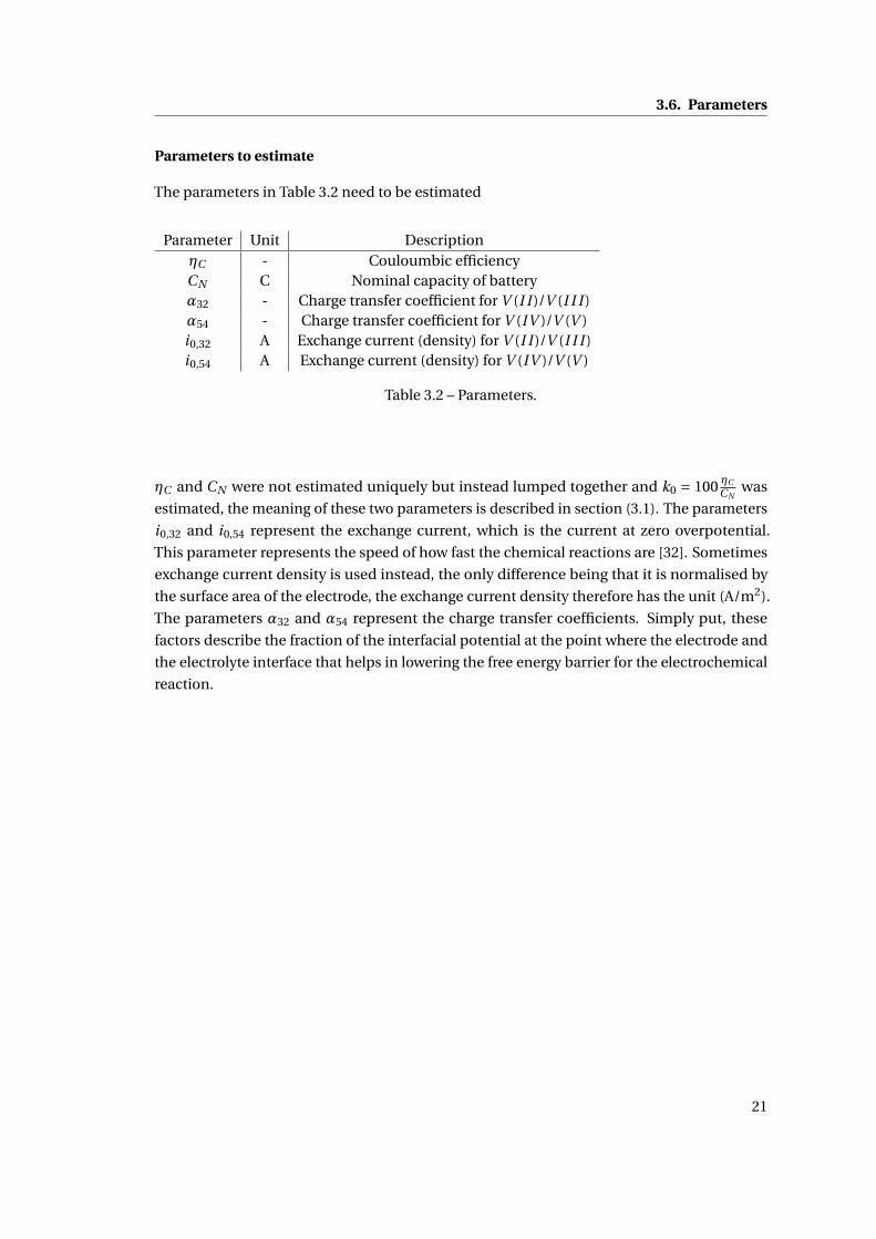
Parameters to estimate

The parameters in Table 3.2 need to be estimated

Parameter Unit DescriptionηC - Couloumbic efficiencyCN C Nominal capacity of batteryα32 - Charge transfer coefficient for V (I I )/V (I I I )α54 - Charge transfer coefficient for V (IV )/V (V )i0,32 A Exchange current (density) for V (I I )/V (I I I )i0,54 A Exchange current (density) for V (IV )/V (V )

Table 3.2 – Parameters.

ηC and CN were not estimated uniquely but instead lumped together and k0 = 100 ηC

CNwas

estimated, the meaning of these two parameters is described in section (3.1). The parameters

i0,32 and i0,54 represent the exchange current, which is the current at zero overpotential.

This parameter represents the speed of how fast the chemical reactions are [32]. Sometimes

exchange current density is used instead, the only difference being that it is normalised by

the surface area of the electrode, the exchange current density therefore has the unit (A/m2).

The parameters α32 and α54 represent the charge transfer coefficients. Simply put, these

factors describe the fraction of the interfacial potential at the point where the electrode and

the electrolyte interface that helps in lowering the free energy barrier for the electrochemical

reaction.

21

4 Parameter estimation and validation

4.1 Methods

The estimation problem is the following. Given a set of measurements for a system, a model

F (t , x, x, z,u, p) with measurable output ymodel (t , p) find the parameters p that solves the

following problem

minimizep

n∑i=1

||ymeasur ed (ti )− ymodel (p)||2Q

subject to p ∈P

(4.1)

where Q is a positive definite weighting matrix, P is the feasible set and ti ∈ [t0, t f ] is the time.

Furthermore

ymodel (p) = h(x, z,u, p) (4.2)

is the output of the model for the system. It is assumed that the input signal u is known over

[t0, t f ] and ymeasur ed (ti ) is given data also known over [t0, t f ].

4.1.1 Linear estimates

In the special case where the parameter is scalar and appears linearly in the equations and the

domain P is unbounded, then P =R and the estimate can be written explicitly [23]. Assume

the unknown scalar parameter p is involved in an equation of the form

yi = p · xi (4.3)

23

Chapter 4. Parameter estimation and validation

where measurements y = (y1, . . . , yn) and x = (x1, . . . , xn) are available. The estimate p of p can

be found by first setting up the overdetermined linear system of equationsx1...

xn

︸︷︷︸

=:A

p =

y1...

yn

︸︷︷︸

=:b

(4.4)

Then the estimate is found by forming the normal equations, i.e. by left multiplying both sides

with AT yielding

ATA ·p = ATb (4.5)

Finally the estimate is found to be

p = (ATA)−1 ATb (4.6)

from the least squares method.

4.1.2 Estimation for a DAE system

The case where parameters appearing in a nonlinear DAE model need to be estimated is

discussed. The estimation problem will be rewritten as an optimization problem and a

numerical optimization solver will be used. For the optimization solver it will be required

to provide a function that computes the objective function value. The optimization solver

requires an initial guess of p. Due to the nonlinearity of the system, the optimal p obtained

may depend on the initial guess since the optimization problem is not convex. Let p be the

vector of parameters to be estimated. Also, define a set P which the parameters p belong to.

Let q(p) be the objective function value for a certain parameter set. Let the nonlinear DAE be

expressed by F (x, x, z,u, p) = 0 with u known. Then, the estimation problem is the following

optimization problem

minimizep

∑k∈K

wk (n∑

i=1||y (k)

measur ed (ti )− ymodel (u(k), p)||22)︸︷︷︸=q(p)

subject to F (x, x, z,u, p) = 0

(x(t0), z(t0)) = (x0, z0) given

p ∈P

(4.7)

where, K is the set of data series used for estimation, [t (k)0 , t (k)

f ] is the estimation horizon

for set k, wk is the weight on data series k and u(k) is the known power level. Each time the

objective function value is computed the DAE system F (x, x, z,u) = 0 needs to be solved for

24

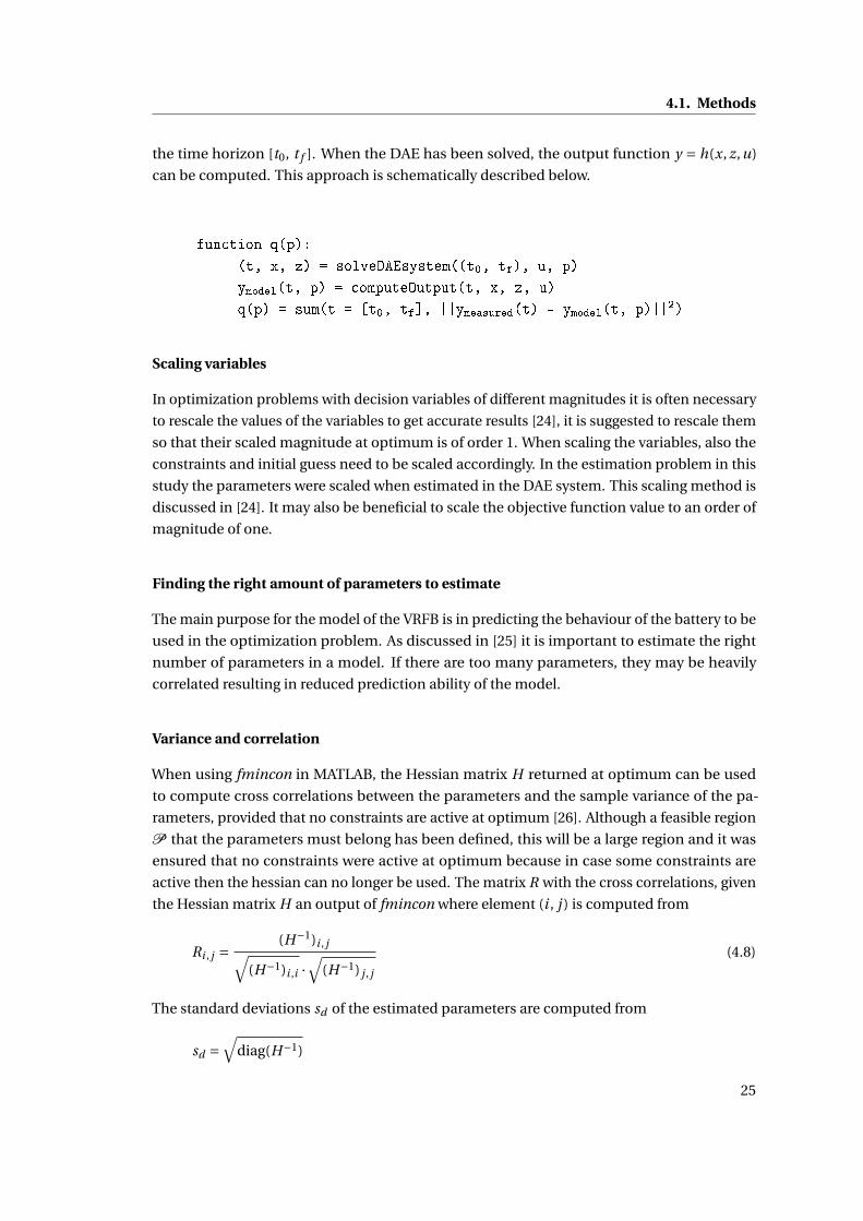
4.1. Methods

the time horizon [t0, t f ]. When the DAE has been solved, the output function y = h(x, z,u)

can be computed. This approach is schematically described below.

function q(p):

(t, x, z) = solveDAEsystem((t0, tf), u, p)

ymodel(t, p) = computeOutput(t, x, z, u)

q(p) = sum(t = [t0, tf], ||ymeasured(t) - ymodel(t, p)||2)

Scaling variables

In optimization problems with decision variables of different magnitudes it is often necessary

to rescale the values of the variables to get accurate results [24], it is suggested to rescale them

so that their scaled magnitude at optimum is of order 1. When scaling the variables, also the

constraints and initial guess need to be scaled accordingly. In the estimation problem in this

study the parameters were scaled when estimated in the DAE system. This scaling method is

discussed in [24]. It may also be beneficial to scale the objective function value to an order of

magnitude of one.

Finding the right amount of parameters to estimate

The main purpose for the model of the VRFB is in predicting the behaviour of the battery to be

used in the optimization problem. As discussed in [25] it is important to estimate the right

number of parameters in a model. If there are too many parameters, they may be heavily

correlated resulting in reduced prediction ability of the model.

Variance and correlation

When using fmincon in MATLAB, the Hessian matrix H returned at optimum can be used

to compute cross correlations between the parameters and the sample variance of the pa-

rameters, provided that no constraints are active at optimum [26]. Although a feasible region

P that the parameters must belong has been defined, this will be a large region and it was

ensured that no constraints were active at optimum because in case some constraints are

active then the hessian can no longer be used. The matrix R with the cross correlations, given

the Hessian matrix H an output of fmincon where element (i , j ) is computed from

Ri , j =(H−1)i , j√

(H−1)i ,i ·√

(H−1) j , j

(4.8)

The standard deviations sd of the estimated parameters are computed from

sd =√

diag(H−1)

25


With this information, we can determine how good the estimates are and if we need to reduce

the number of parameters, in case of high correlation.

4.2 Results

Measurement data

We present here the data that were obtained from measurements of the physical system.

The data includes state of charge, current, AC power, DC power and output voltage. Two

data sets were available. The data contains one cycle of charging with a low initial SOC of

around 10% until charged to around 85%. For discharge cycles, the initial SOC is around 85%

and measurements are obtained until the SOC is about 10%. The first data set contained

measurements with AC power levels 2, 4, 5, 6, 8, 10, 15 (kW). The second data set contained

measuremnts with AC power levels 4, 5, 6, 7, 8, 9, 10 (kW). Both comprised charge and

discharge measurements at the same power. The first data set was obtained a few months

before data set 2 and although no changes where made to the battery, due to the time difference

the performance of the battery may have been affected. Some sample data are shown in Table

4.1. Only DC power will be used in this study.

time (min) SOC (%) current (A) voltage (V) AC power (W) DC power (W)0 73 100 53.5 8000 79001 73.5 99 53.8 8000 79002 74 98 54.1 8000 7900...

......

......

...

Table 4.1 – Sample data.

Estimation of k0

Denote k0 to be the final estimate of k0, k0 will be defined as the mean of all estimated values

of k0. For each data series one value of k0 was determined from data by discretization of

equation (3.1), yielding the relation

sk+1 = sk +k0ik∆k

where ∆k = tk − tk−1 is the difference in time between two measurement points and tk is the

time at measurement point k, ik is the current at measurement point k and sk is the state of

charge at measurement point k. Data of charge and discharge cycles were available containing,

among others, the values (tk , sk , ik ) for n data points. Then k0 was obtained using the least

squares method to the following overdetermined linear system of equations,

26

4.2. Results

i1∆1

...

in−1∆n−1

︸︷︷︸

=:A

k0 =

s2 − s1

...

sn − sn−1

︸︷︷︸

=:b

(4.9)

where n is the number of data points in a data set. Using directly equation (4.6) we obtain the

estimate. For each data series available, which included charge and discharge data for power

levels 2, 4, 5, 6, 8, 10, 15 (kW), one specific value of k0 was estimated. Then k0 was taken as

the mean of all the estimates. Note that this value of k0 assumes the SOC is measured in the

interval [0, 100] (%) and the current in (A).

For each data series one value of k0 was found as listed in Table 4.2.

Charge or discharge Power (kW) k0

Charge 7 0.00204Charge 8 0.00196Charge 9 0.00195Charge 10 0.00197

Discharge 7 0.00202Discharge 8 0.00195Discharge 9 0.00190Discharge 10 0.00195

Table 4.2 – Estimates for different power values.

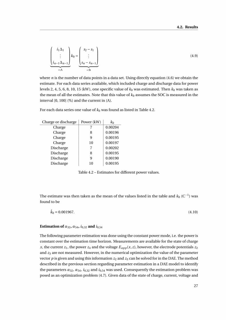
The estimate was then taken as the mean of the values listed in the table and k0 (C−1) was

found to be

k0 = 0.001967. (4.10)

Estimation of α32, α54, i0,32 and i0,54

The following parameter estimation was done using the constant power mode, i.e. the power is

constant over the estimation time horizon. Measurements are available for the state of charge

x, the current z1, the power z4 and the voltage Eapp (x, z), however, the electrode potentials z2

and z3 are not measured. However, in the numerical optimization the value of the parameter

vector p is given and using this information z2 and z3 can be solved for in the DAE. The method

described in the previous section regarding parameter estimation in a DAE model to identify

the parameters α32, α54, i0,32 and i0,54 was used. Consequently the estimation problem was

posed as an optimization problem (4.7). Given data of the state of charge, current, voltage and

27


power over some time interval [t0, t f ] for different power settings for charge and discharge

cycles the parameters were estimated. Define p,

p = (α32,α32, i0,32, i0,54)

to be the vector of parameters. The objective function f (p) was set to

q(p) = ∑k∈K

wk (n∑

i=1||E (k)

appmeasur ed(ti )−Eappmodel

(u(k), p)||22) (4.11)

so the output voltage is taken into account in the objective function and the other measurable

quantities, i.e. state of charge and current are not used. Note that since the power is set to a

fixed value and the SOC is directly related to the current and the initial SOC is known, as long

as the voltage is correct then the current will follow and thus also the SOC. We then define the

feasible set P to be chosen so that α32 and α54 are restricted to the interval [ε, 1−ε] and i0,32

and i0,54 are restricted to the interval [ε, 100], with ε= 10−3. We note that from literature [32] it

must hold that α32 ∈ [0,1] and α54 ∈ [0,1].

Initial results showed very high correlations between the parameters. Thus it was decided

to fix α32 and α54 to the values that were obtained when estimating all four parameters and

then only perform the estimation procedure with two free parameters. Internal experiments

suggest a value for α32 close to what was obtained here, whereas the experimental value of α54

is more uncertain [27]. In fact, it is often possible to approximate the parameters α54 and α54

by setting them to 0.5 [32]. The following parameter values listed in Table 4.3, with standard

deviations were obtained and later used in simulating the system.

Parameter Value Standard deviation Unit Descriptionα32 0.144 - - Charge transfer coefficient for V (I I I )/V (I I )α54 0.544 - - Charge transfer coefficient for V (V )/V (IV )i0,32 0.2555 0.00479 A Exchange current (density) for V (I I I )/V (I I )i0,54 0.000304 7.11·10−7 A Exchange current (density) for V (V )/V (IV )

Table 4.3 – Sample data of measurements from the battery.

The correlations between the parameters as obtained from the optimization are listed in Table

4.4.

i0,32 i0,54

i0,32 1 -0.238i0,54 -0.238 1

Table 4.4 – Sample data of measurements from the battery.

28

4.3. Model validation

The cross correlation (which is in the interval [-1, 1]) is close enough to 0 (zero) to suggest that

it is acceptable to fit two parameters for this model.

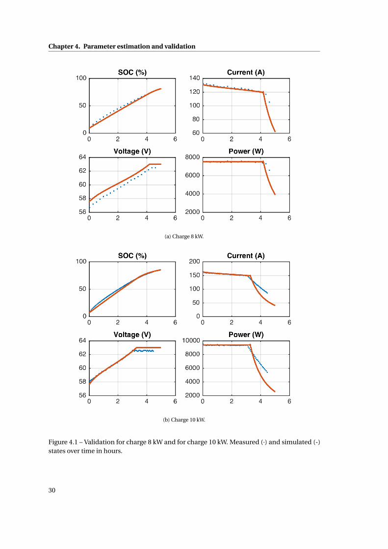
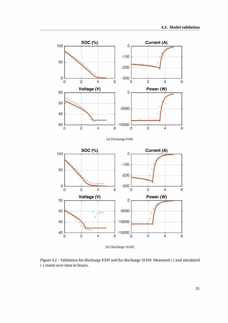
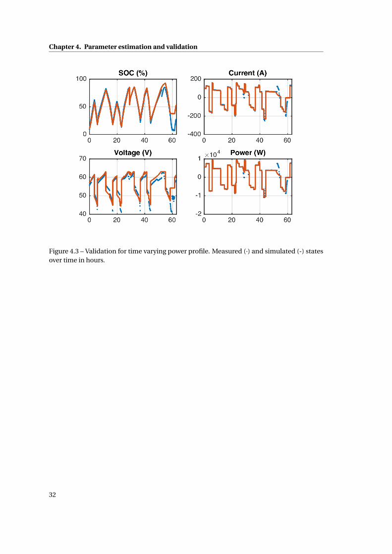
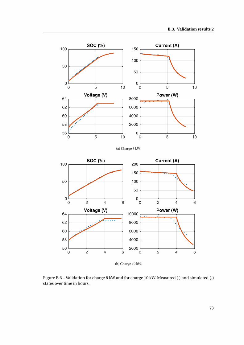
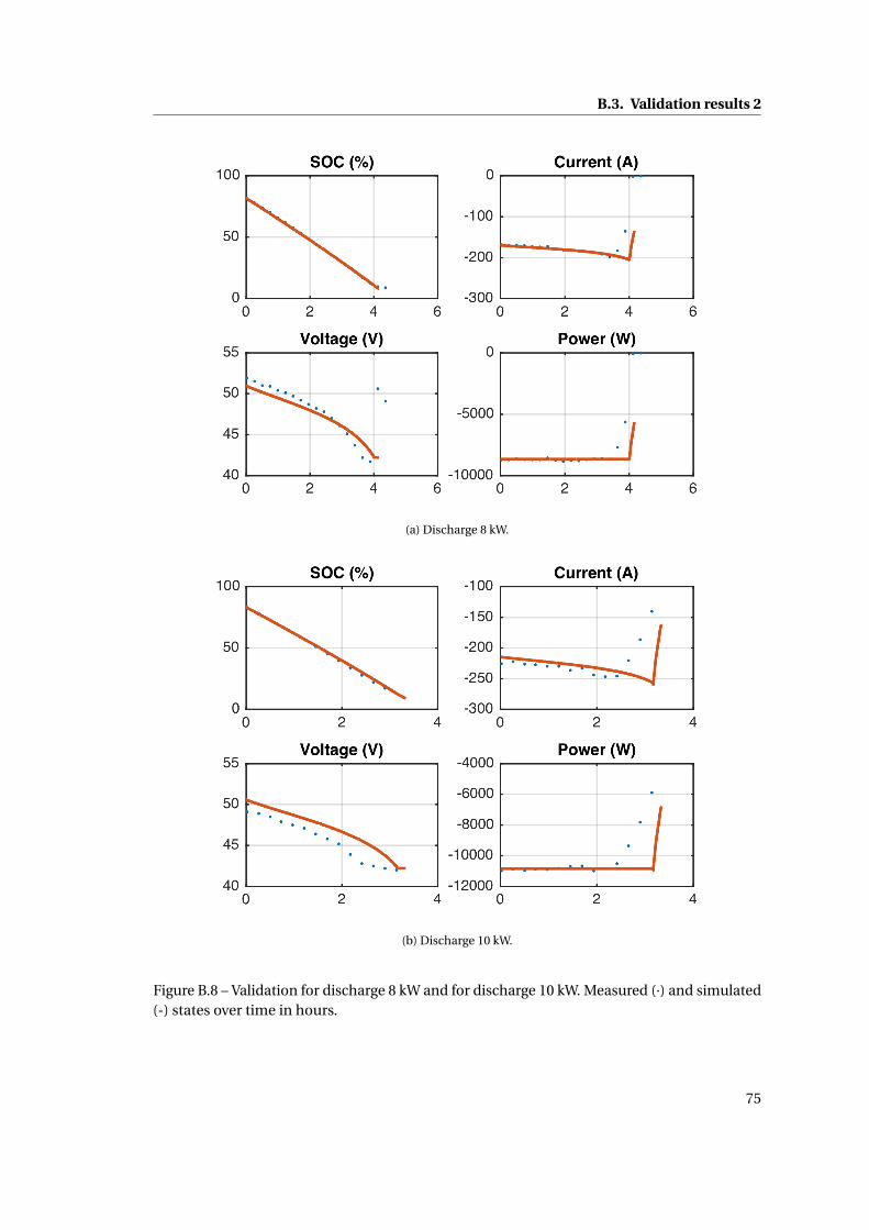
4.3 Model validation

Additional experimental data, not the same data that were previously used for identification,

were provided and the model was evaluated against the data. The strongest verification of the

prediction power of the model is obtained when comparing the model to additional data that

had not been used for estimation purposes. The results of this validation are presented here.

Validation results

The simulated model is evaluated against data that were not used to estimate the parameters.

In the optimal control strategy of the battery, the power is expected to change frequently, the

time varying power profile shows good fit between data and model.

Discussion

In conclusion it seems the predictions of the state of charge are reasonable, whereas the

predictions on voltage are sometimes off with a few volts, about 0-3 (V). It is important to

keep in mind that when the voltage hits the thresholds the regime of the battery changes and

the current model is not always capable of predicting that switch on time. We also note that

restriciting ourselves to only having one set of parameters that are the same for all power

levels and for both charge and discharge reduces the overall accuracy of the model. The time

varying power profile shows good fit and when optimizing the battery operation mode it is

expected that the power will change freqeuently showing a similar trend as the time varying

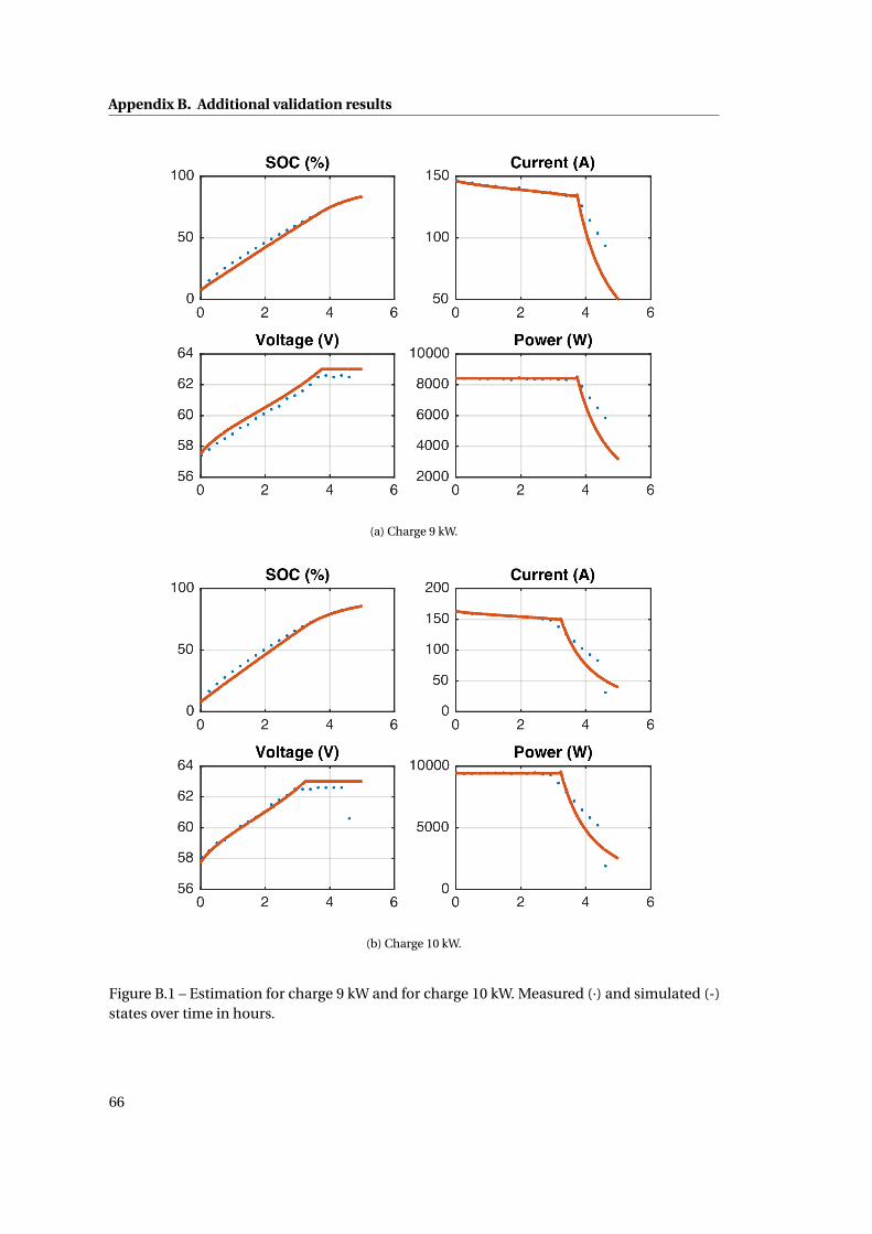
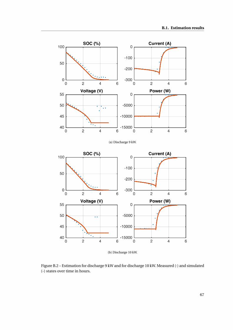
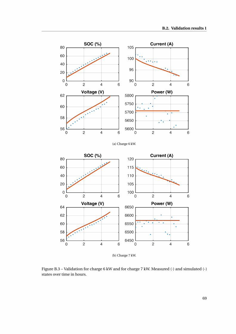
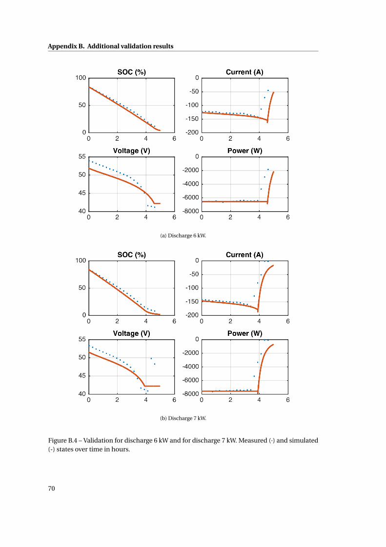
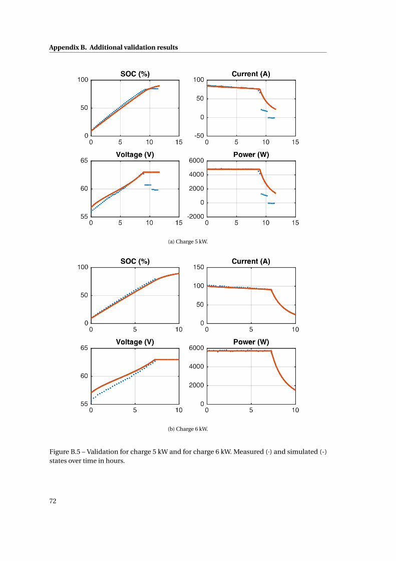
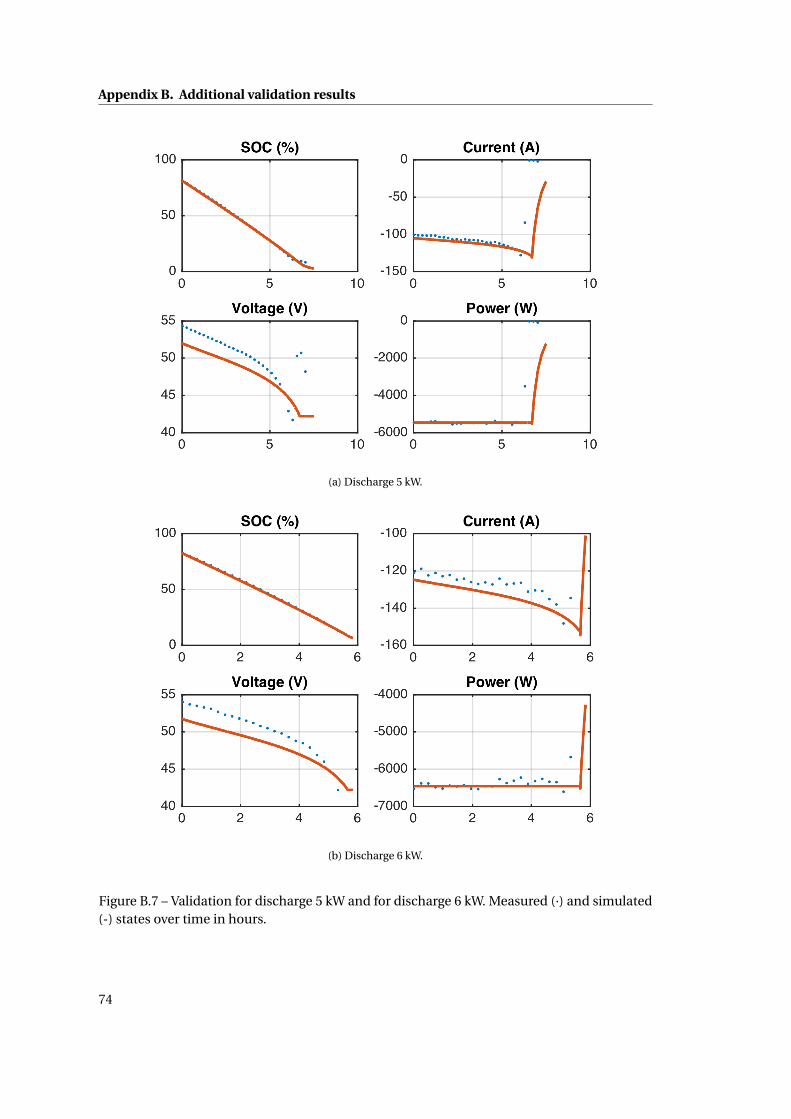
power profile, thus it seems the model is good enough. Additional validation results are listed

in the appendix without a discussion.

29


(a) Charge 8 kW.

(b) Charge 10 kW.

Figure 4.1 – Validation for charge 8 kW and for charge 10 kW. Measured (·) and simulated (-)states over time in hours.

30

4.3. Model validation

(a) Discharge 8 kW.

(b) Discharge 10 kW.

Figure 4.2 – Validation for discharge 8 kW and for discharge 10 kW. Measured (·) and simulated(-) states over time in hours.

31


Figure 4.3 – Validation for time varying power profile. Measured (·) and simulated (-) statesover time in hours.

32

5 Optimization

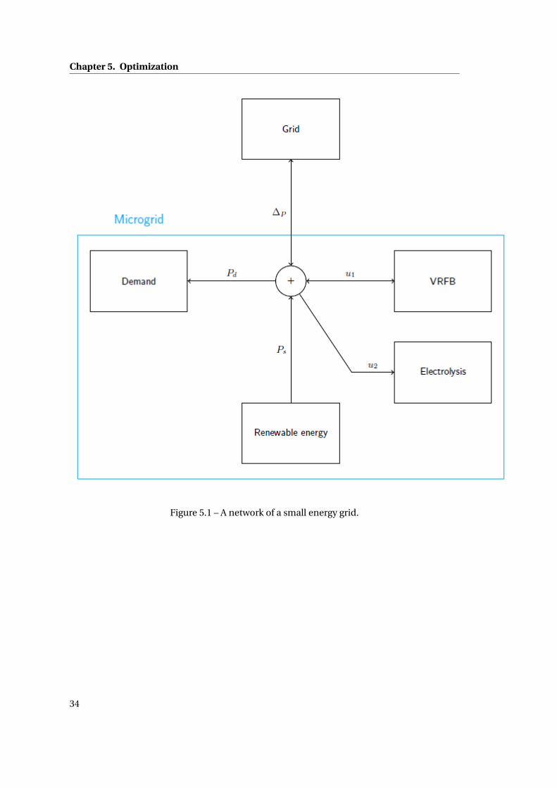
5.1 The electrical network

The following situation is considered, a small utilities company owns renewable means of

production such as solar panels or wind turbines. The company has a contract with local

residents of a town to provide energy to them. Since these sources of electricity are highly

fluctuating and cannot be produced at request, the company has a battery connected to

their grid. In this study they also have hydrogen storage in case the battery should be fully

charged and there is an excess of renewable energy. In case the renewable energy and battery

cannot provide enough energy additional power from the grid may be used. The operator

of the grid wishes to maximize the operational performance of the network with respect to

some performance metric that will be defined shortly. For instance the operator could be

interested in maximizing the profit of operating the network. We define the microgrid to be all

the physical systems belonging to the company and its customers and the grid to be public

network where other companies trade electricity. The network in Figure 5.1 illustrates this

arrangement. Regarding the battery and the grid, define the following variables

u1 Power applied to the battery (instead of previously used u)

u2 Power for hydrogen generation

Ps Power generated from renewable sources (supply)

Pd Power demanded by consumers (demand)

For simplicity we have assumed that there are no losses and no disturbances in the network.

Recall that z4 was used to denote the power of the battery and u1 only when the battery

operates in power driven mode, however, when optimizing the battery, the power level is

expected to switch frequently and the battery will seldom reach the voltage thresholds.

33

Chapter 5. Optimization

Figure 5.1 – A network of a small energy grid.

34

5.2. Constraints

5.2 Constraints

The constraints in the system are those that arise due to physical limitations on the battery

and the dynamics of the VRFB and the electrolysis.

Dynamic constraints on the battery

The DAE model (3.25) must be fulfilled.

Limits on differential states

The SOC x, can theoretically range in the interval [0, 100] (%), but will only be operated in the

interval [10, 85] (%). This yields

10 ≤ x ≤ 85. (5.1)

Limits on algebraic states

The voltage level on the battery Eapp (x, z) is restricted to the interval [42,63] (V)

42 ≤ Eapp (x, z) ≤ 63. (5.2)

Limits on control

The power level on the battery u1 is restricted to the interval [-15, 15] (kW),

−15 ≤ u1 ≤ 15 (5.3)

where the sign convention states that the power is negative when discharging and positive

when charging. Similarly, limits on the amount of hydrogen that can be produced must be

introduced

0 ≤ u2 ≤ Hmax (5.4)

where Hmax = 14 (kW) and depends on the specific hydrogen generator and this limit was

obtained from the specific equipment.

Balance in the network

We assume throughout that there are no losses and no disturbances. The balance b, between

supply and demand in the considered grid is

b = Ps −Pd (5.5)

35


From figure 5.1, overall power balance in the network requires that

∆P = b −u1 −u2 (5.6)

The sign convention states that u1 is positive if the battery is being charged and negative if

the battery is being discharged. Similarly, power going into the network is positive and power

going out of the network is negative. Thus u2, Ps and Pd are positive and ∆P which is what

must be bought from or sold to the grid can be positive or negative. We notice that if ∆P ≥ 0

then energy is sold to the main grid and if ∆P ≤ 0 then energy must be bought from the main

grid. These constraints on Ps and Pd will be enforced by given data so it is not necessary to put

bounds on them. Ps and Pd will be specified as time varying known functions and different

scenarios will be considered in the next chapter.

Final state of charge

It will be investigated to enforce the same final level of the state of charge as the initial one

x(t f ) = x(t0). (5.7)

The state of charge at final time could also be free.

5.3 Objective function

The optimization problem will be formulated as a minimization problem. Let L denote the

cost term over the entire time horizon (Lagrange term) and E denote the cost term at the final

time (Mayer term). The objective function J is then the sum of these terms

J (x0, z0,u(·)) = E(t f , x(t f ), z(t f ))+∫ t f

t0

L(t , x(t ), z(t ),u(t ))d t (5.8)

5.3.1 Cost at final time

Since the planning presented here is restricted to a limited time horizon it would clearly be

beneficial to deplete the battery at the end of the cycle, however, this would not necessarily be

optimal for times after the planning horizon. Thus by introducing a value on energy left in the

battery after the final time this problem can be reduced. This can be expressed as

E(·) =α f · x(t f ) (5.9)

where x(t f ) is the SOC at the final time for an attributed weight α f . However, for this study it

was decided to instead have a hard constraint for the final value of the state of charge (5.7).

36

5.3. Objective function

5.3.2 Cost over horizon for different objectives

We discuss here the optimal control problem for various objectives, e.g. maximizing profit or

minimizing the interaction with the main grid. We could also consider a weighted sum of the

objective functions presented below.

Minimize vertical net load

This objective is referred to as minimizing the vertical net load or minimzing the vertical grid

load. In this objective we aim at minimizing the amount of energy that has to be bought

from the grid. In literature the problem of peak shaving is common. This consists of storing

energy when consumption is less than demand and used at high demand or peak hours. Since

the electricity produced in the microgrid is renewable, this objective also attempts to reduce

emissions since the electricity from the grid cannot be guaranteed to be climate neutral. This

objective of minimizing the vertical net load is essentially the same as maximizing the self

consumption commonly studied in literature, which comes down to operating the battery so

as to maximize its usage and thus simultaneously minimizing the amount of energy bought

from or sold to the main grid. The cost function is

L(·) = ||∆P (t )||2Q (5.10)

where Q is a positive definite weighting matrix. We could here consider different norms, e.g.

1-norm, 2-norm or ∞-norm. Charge balance is required

∆P (t ) = Ps(t )−Pd (t )−u1(t )−u2(t ) ∀t ∈ [t0, t f ]. (5.11)

We aim at minimizing the cost function J (·) = E(·)+∫ t f

t0L(·)d t . In this optimization problem

the electrolysis for H2 generation will be used when the battery is fully charged and there is an

excess of renewable energy produced, which can be formulated

u2(t ) =0 if ∆P ≤ 0∨x < 85

∆p if ∆P ≥ 0∧x ≡ 85(5.12)

Extension of this problem We may also consider a modification of the above problem where

we need to supply a demand for a certain time horizon only with energy from the renewable

sources and from the battery i.e. the microgrid is not connected to the grid. Let t0 be the initial

time and t f the final time, also define the intermediate time tm such that tm > t0 and t f > tm .

Then the first time horizon [t0, tm] acts as a warm up period where the microgrid is connected

to the grid and the battery can be charged to provide enough energy for the period (tm , t f ].

The objective function is the same as before over the time horizon [t0, t f ], charge balance is

37


required, as previously

∆P = Ps −Pd −u1 −u2 ∀t ∈ [t0, t f ] (5.13)

But we also introduce the constraint

∆P ≡ 0 ∀t ∈ (tm , t f ] (5.14)

so that the microgrid is operated autonomously in the second part of the time horizon. We

note that it is important to choose tm such that the resulting problem is feasible with respect

to the production and consumption plans. This is sometimes referred to as islanded operation

in the literature.

Maximizing profit

We also consider the problem of maximizing the profit associated to the operation of the

microgrid. The cost function is

L(·) = c(t ) ·∆P + cH2 ·α ·u2 (5.15)

c(t ) is the sell or buy price of electricity at the grid at hour t , ∆p is the amount of energy sold or

bought from/to the grid. α is the efficiency factor of the electrolysis, we have from before that

α= 0.5 and u2 is the amount of power (W) that is used to produce hydrogen and cH2 = 0.02

is the price for hydrogen (CHF/kWh) which is assumed to be fixed. We comment that the

hydrogen price is lower than the buy price of the grid, thus only electricity from the renewable

generation is expected to be used for producing hydrogen. By making use of this formulation

we do not need to include the dynamic equation for electrolysis discussed in the beginning of

this chapter, the alternative formulation is discussed below, which is needed if the hydrogen is

modeled with more complicated dynamics. We will also have that

c(t ) =csel l (t ) if ∆P > 0

cbuy (t ) if ∆P ≤ 0(5.16)

Recall if ∆P > 0 then there is an excess of power available and if ∆P < 0 there is a shortage of

power. We aim at maximizing the cost function J (·) = E(·)+∫ t f

t0L(·)d t or equally minimizing

−J(·). We also assume that there are no cost for providing energy to the network, known as

feed in tariffs. Also note that if the battery is not empty at the final time, then there is value

from this electricity. Thus as final cost we take E as in equation (5.9).

Alternative formulation Since the hydrogen price was assumed constant we may formulate

this differently by putting the profit from hydrogen as a terminal cost which incorporates the

38

5.3. Objective function

profit from all hydrogen produced over the time horizon

E(·) = cH2 · xH (5.17)

where cH2 is the fixed H2 price and xH is the amount of H2 produced during the considered

period. Then the cost over the time horizon is

L(·) = c(t ) ·∆p (5.18)

We also need to incorporate the dynamic equation for the electrolysis (3.31) as a constraint of

the optimal control problem.

Minimize emissions of green house gases

L(·) = ||min(∆P (t ),0)||2Q (5.19)

where

min(∆P (t ),0) =∆P (t ) if ∆P (t ) < 0

0 if ∆p ≥ 0(5.20)

Thus there is no penalty on selling power, but there is a penalty on buying power which is

motivated by the assumption that the sold power is renewable whereas the bought power is

not renewable.

Preventing aging of battery

We may also consider the long term cost of operating the battery to reduce aging of the

battery, for each charge and discharge cycle. The battery deteriorates after usage in certain

conditions and this could be included in the optimization formulation. In the literature this

problem has been attempted by avoiding too high state of charge values and also by limiting

the temperature of the battery [12], however for this study we assume a constant temperature.

Maximizing the state of charge

We may also consider maximizing the state of charge of the battery, either at all times or at the

final time while meeting customer demands. For this problem we could also take electricity

prices into account. In the first case we get the cost function

L(·) = ||xmax −x(t )||2 (5.21)

39


where xmax = 85 is the maximal state of charge, E(·) = 0. In the latter case we get the cost

function

E(·) = x(t f ) (5.22)

and L(·) = 0. We aim at maximizing the cost function. This objective will typically lead to

a high amount of energy being bought from the main grid. This issue can be reduced by

introducing limits on the amount that can be bought at each time ∆P (t ) ≤β ∀t ∈ [t0, t f ], for

some suitable β ∈R.

Weighting all objectives together

It could also be interesting to consider as objective function a weighted sum of all the objectives

presented above.

5.4 Optimal control problem

The full OCP is now presented.

minimizeu(·)

E(t f , x f , z f )+∫ t f

t0

L(t , x, z,u)d t

subject to x = f (x, z,u) dynamic constraints, eq (3.26)

0 = g (x, z,u) algebraic constraints eq (3.27)

10 ≤ x ≤ 85 limits on state of charge (%)

42 ≤ Eapp (x, z) ≤ 63 limits on voltage (V)

−15 ≤ u1 ≤ 15 limits on power (kW)

0 ≤ u2 ≤ 14 limits on power (kW)

∆P = Ps(t )−Pd (t )−u1 −u2 network power balance

x0 given initial state of charge known

(5.23)

Different objectives

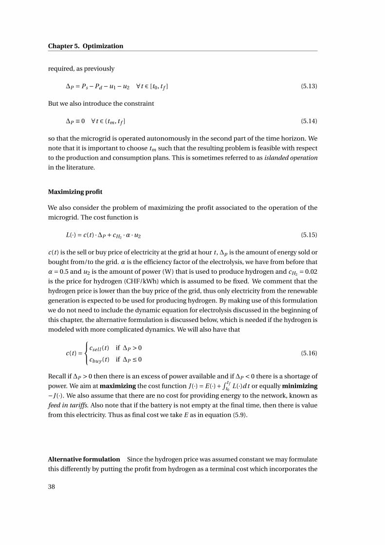
We have considered different objectives in terms of our goal of operating the battery, we here

present the objective functions for those OCPs in Table 5.1 using the notation described in the

previous sections

To limit the scope of this study we restrict ourselves to only consider the first two objectives in

Table 5.1.

40

5.5. Implementation aspects

Comment E LMinimize vertical net load 0 ||∆P (t )||2Q

Maximize profit 0 c(t ) ·∆p + cH2 ·α ·u2

Maximize final SOC x(t f ) 0Maximize SOC 0 ||xmax −x(t )||2

Minimize emissions 0 min(∆P ,0)

Table 5.1 – Different objectives.

5.5 Implementation aspects

The time horizon was chosen to one day since the data have typical trends for a day. The

optimal control problem stated in the previous section is open loop where the consumption-

and production- profiles and the prices are known in advance. Therefore it also proposed

to solve the OCP in a way similar to MPC (Model Predictive Control). The idea is to solve

the OCP over a limited time horizon, then apply the first value of the optimal feedback, let

the dynamics of the system evolve and then iterate this process over the full time horizon.

This is more realisitic, since in reality the accuracy of the forecasts of consumption- and

production- profiles would decrease drastically with time and only the forecast for the next

few hours may be accurate enough. Furthermore this MPC like approach takes the problem

of not prefectly knowing the consumption- and production- profiles into account by only

considering a subinterval of the full time horizon when solving for the optimal feedback. The

approach is sketched below.

Receding horizon OCP

u = solveOCP(t0, t f , data(t0, t f ))

Apply u and evolve dynamics of VRFB

t0 := t0 + ti nc, t f := t f + ti nc

where ti nc is the length of each control interval and data(t0, t f ) are the production, consump-

tion and prices over the interval [t0, t f ], ti nc is the same as the control interval. We note that

for the receding horizon approach the state of charge at final time was free.

Toolbox

The MATLAB toolbox GPOPS II was used to solve the optimal control problem [20].

5.6 Performance metrics

Some metrics for analyzing the results are discussed.

41


Emissions of greenhouse gases

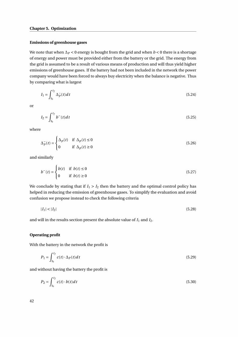
We note that when ∆P < 0 energy is bought from the grid and when b < 0 there is a shortage

of energy and power must be provided either from the battery or the grid. The energy from

the grid is assumed to be a result of various means of production and will thus yield higher

emissions of greenhouse gases. If the battery had not been included in the network the power

company would have been forced to always buy electricity when the balance is negative. Thus

by comparing what is largest

I1 =∫ t f

t0

∆−P (t )d t (5.24)

or

I2 =∫ t f

t0

b−(t )d t (5.25)

where

∆−P (t ) =

∆p (t ) if ∆p (t ) ≤ 0

0 if ∆p (t ) ≥ 0(5.26)

and similarly

b−(t ) =b(t ) if b(t ) ≤ 0

0 if b(t ) ≥ 0(5.27)

We conclude by stating that if I1 > I2 then the battery and the optimal control policy has

helped in reducing the emission of greenhouse gases. To simplify the evaluation and avoid

confusion we propose instead to check the following criteria

|I1| < |I2| (5.28)

and will in the results section present the absolute value of I1 and I2.

Operating profit

With the battery in the network the profit is

P1 =∫ t f

t0

c(t ) ·∆P (t )d t (5.29)

and without having the battery the profit is

P2 =∫ t f

t0

c(t ) ·b(t )d t (5.30)

42

5.6. Performance metrics

We note that if P1 > P2, then the profit is larger when having the battery compared to without.

Negative profit means costs. We also note that for an accurate comparison the cost of the

battery should be taken into account. We suggest to take the average profit of one day in

July and one in December to give an approximate value for profit of an average of the year.

Then knowing the price of the battery, the number of years until the battery pays off can be

determined and hopefully this number is smaller than the expected life length of the battery.

43

6 Results

Due to very long computation times for some problems as well as for limiting the length of this

thesis, we restrict ourselves to consider only a few cases. The cases that will be considered are

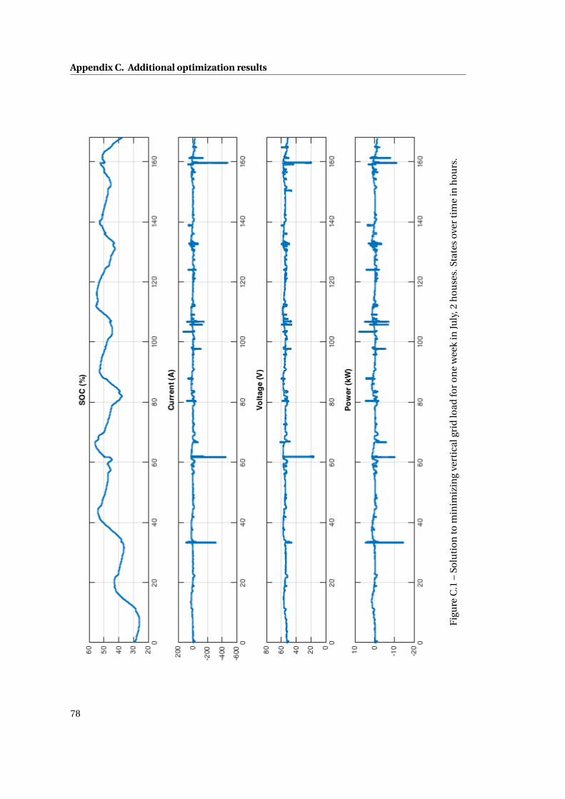
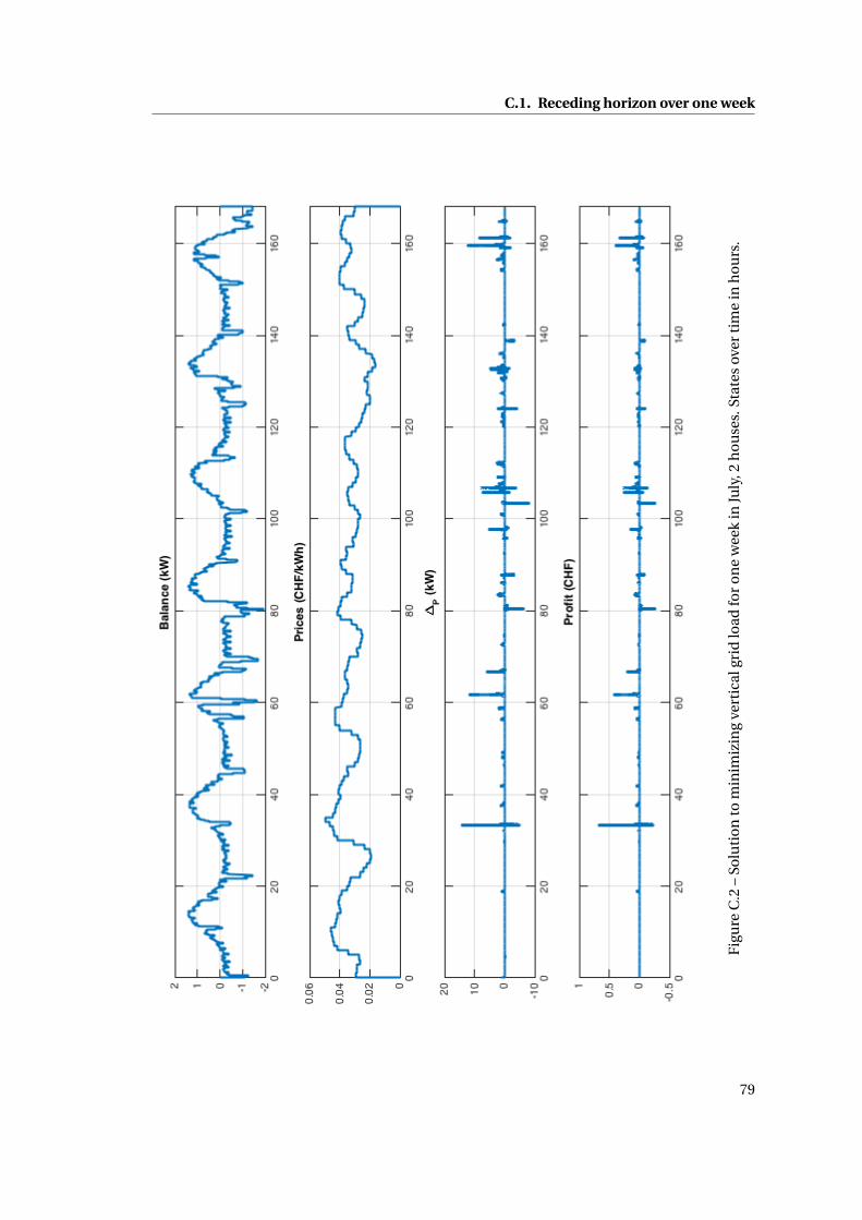
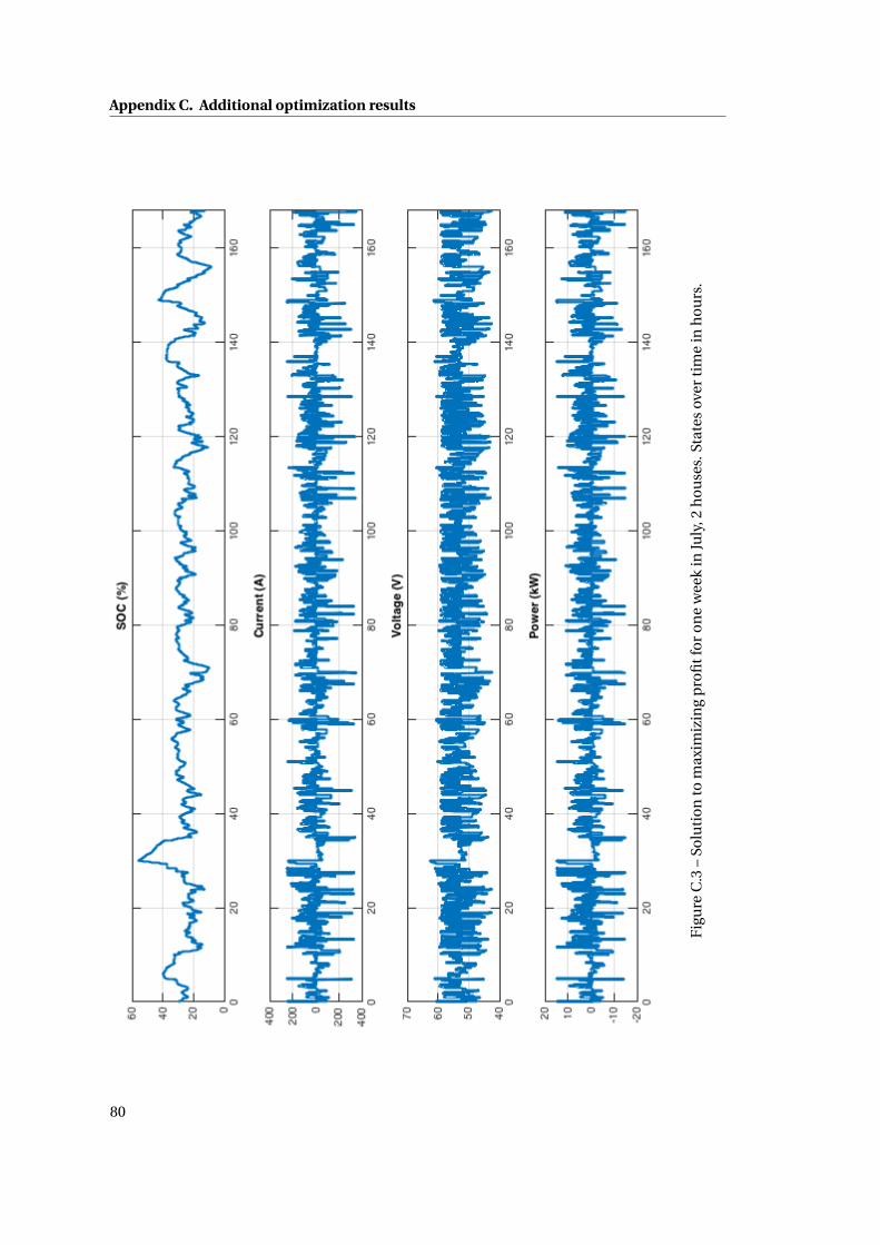
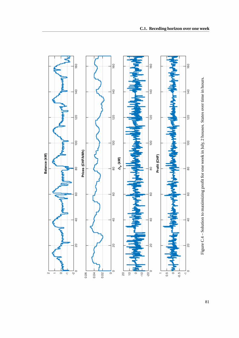
an open loop control policy and a receding horizon approach over one day. In the appendix the

receding horizon approach over one week is included, but without analyzing the performance

metrics. It was attempted to scale up the data significantly to 20 houses instead of 2 houses,

while keeping the battery size the same. The attempts were unsuccessful. Adjusting the

settings in the solver and providing a better initial guess for the optimal solution might have

solved the problem for 20 houses, however, due to long computation times (typically more

than 10 hours on desktop computer) and limited time for the project this was not done.

We note that in the modeling and estimation part of the project it was desired to optimize the

model for power levels around 10 kW. However, in the optimal control policy of the battery

presented in the next sections, the battery is most of the time not operated in this region. One

reason for this is that the data used are not completely accurate, the data have been acquired

from different sources and rescaled to fit to average values of power consumption and demand

but may not adapt completely to the region were the battery is currently installed. Another

reason is that in the considered setup the size of the photovoltaics is of appropriate size for 2

houses and not considered as a big farm operated by the company. Since the photovoltaics are

adapted in size for 2 houses they typically do not produce too much nor too little and therefore

on an average day the balance (difference between supply and demand) should be close to

0 (zero) (W). The customer do not want to buy too many square meters of solar panels to

constantly overpoduce, neither too few square meters to constantly having to buy electricity

from the grid.

6.1 Data

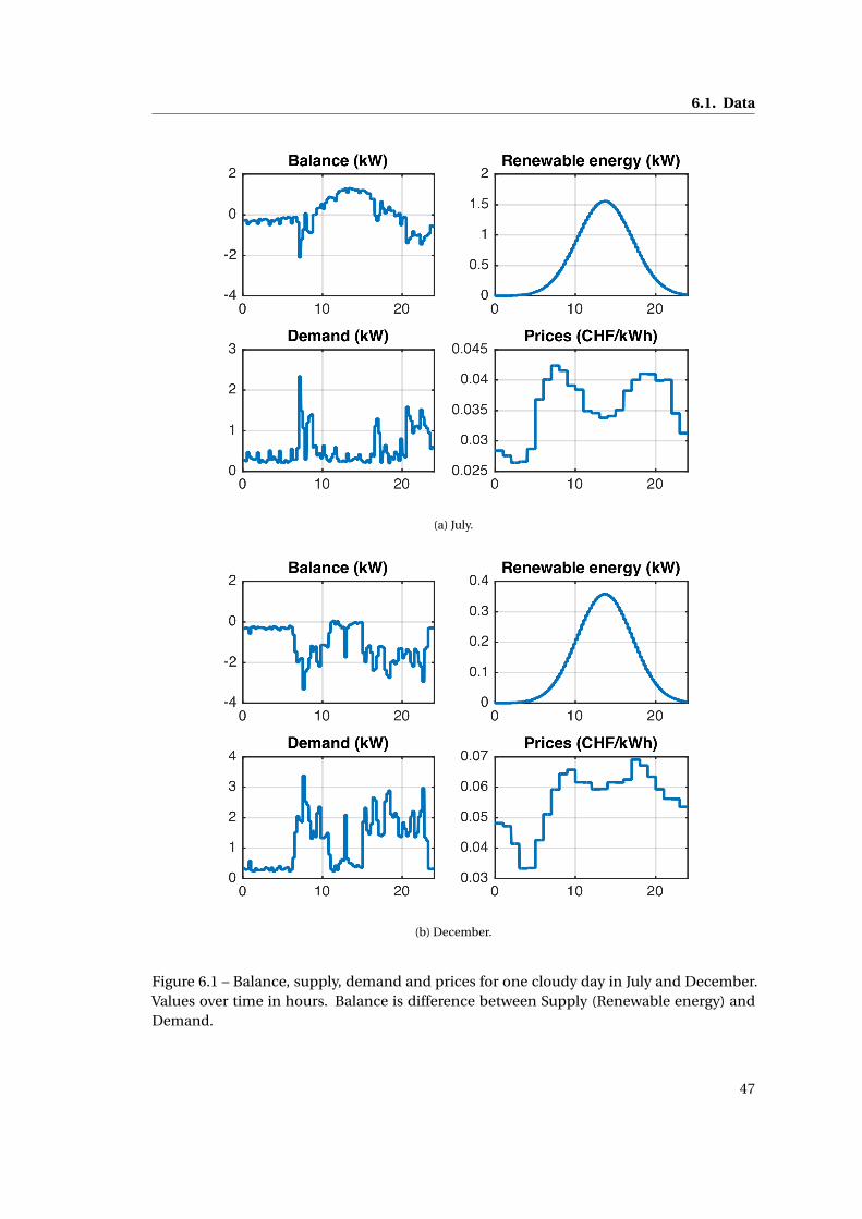
The supply (Renewable energy) is from photovoltaics (solar cells), the data used were de-

termined from measurements [28] but has been smoothed by fitting a Gaussian curve. The

demand was obtained from a time varying profile with measurements every minute during

45

Chapter 6. Results

a day but has been smoothed over 15 minutes due to high fluctuations. The data are from a

house [29] where measurements have been obtained every minute, and has been rescaled so

that the total consumption over one year is that of a Swiss standard house, that is 4500 (kWh).

The price of electricity is a time varying profile were prices are constant during one hour

[30]. The VRFB under study is suitable for ca 2 houses and 40-50 m2 solar panels. Data was

available for all months of the year but July and December were chosen since they represent

the two extremes of the year. July is the sunniest period of the year and is associated with a low

consumption, whereas December has the fewest sun hours and presents high consumption.

46

6.1. Data

(a) July.

(b) December.

Figure 6.1 – Balance, supply, demand and prices for one cloudy day in July and December.Values over time in hours. Balance is difference between Supply (Renewable energy) andDemand.

47

Chapter 6. Results

6.2 Open loop optimization over one day

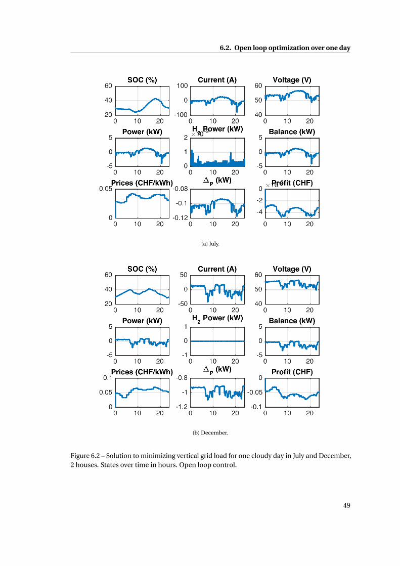
The initial state of charge was chosen to x(t0) = 30%, the final state of charge was enforced to

be the same as the initial, x(t f ) = x(t0). The two objectives of minimizing vertical grid load

and maximizing profit were investigated. The data were scaled for 2 houses. Data for one day

in July was used as well as data for one day in December. By open loop it is meant that the

feedback is computed for the whole day at once.

48

6.2. Open loop optimization over one day

(a) July.

(b) December.

Figure 6.2 – Solution to minimizing vertical grid load for one cloudy day in July and December,2 houses. States over time in hours. Open loop control.

49

Chapter 6. Results

(a) July.

(b) December.

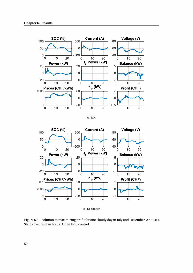
Figure 6.3 – Solution to maximizing profit for one cloudy day in July and December, 2 houses.States over time in hours. Open loop control.

50

6.3. Receding horizon optimization over one day

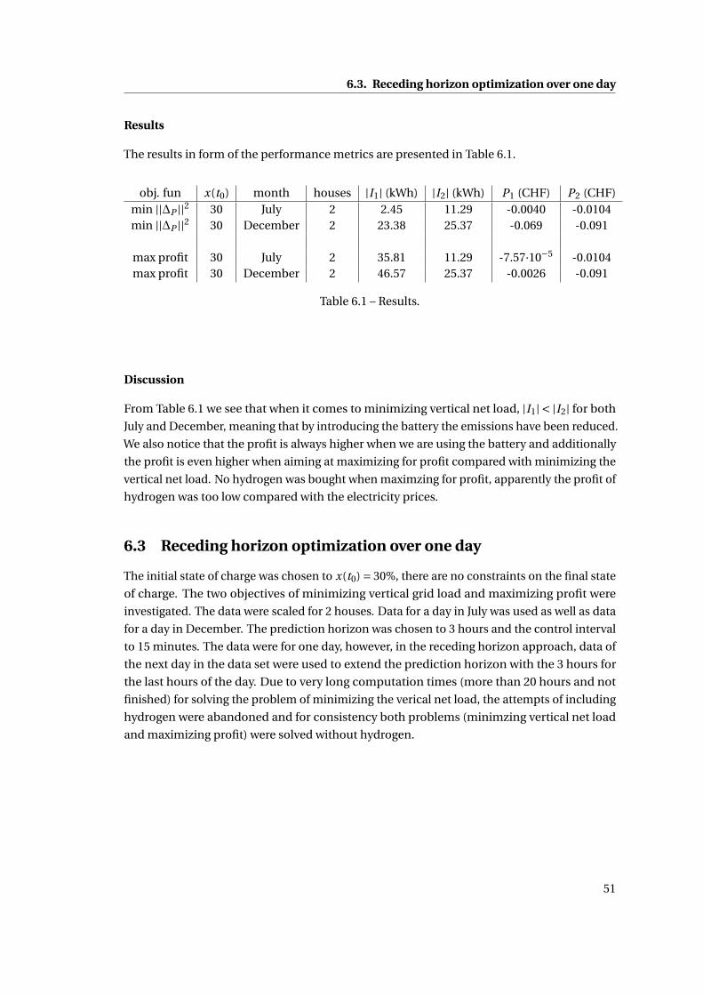
Results

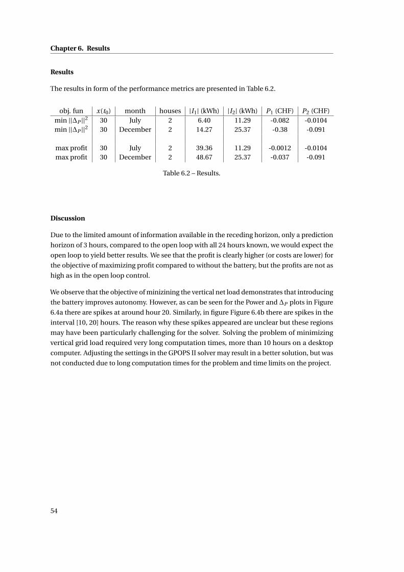
The results in form of the performance metrics are presented in Table 6.1.

obj. fun x(t0) month houses |I1| (kWh) |I2| (kWh) P1 (CHF) P2 (CHF)min ||∆P ||2 30 July 2 2.45 11.29 -0.0040 -0.0104min ||∆P ||2 30 December 2 23.38 25.37 -0.069 -0.091

max profit 30 July 2 35.81 11.29 -7.57·10−5 -0.0104max profit 30 December 2 46.57 25.37 -0.0026 -0.091

Table 6.1 – Results.

Discussion

From Table 6.1 we see that when it comes to minimizing vertical net load, |I1| < |I2| for both

July and December, meaning that by introducing the battery the emissions have been reduced.

We also notice that the profit is always higher when we are using the battery and additionally

the profit is even higher when aiming at maximizing for profit compared with minimizing the

vertical net load. No hydrogen was bought when maximzing for profit, apparently the profit of

hydrogen was too low compared with the electricity prices.

6.3 Receding horizon optimization over one day

The initial state of charge was chosen to x(t0) = 30%, there are no constraints on the final state

of charge. The two objectives of minimizing vertical grid load and maximizing profit were

investigated. The data were scaled for 2 houses. Data for a day in July was used as well as data

for a day in December. The prediction horizon was chosen to 3 hours and the control interval

to 15 minutes. The data were for one day, however, in the receding horizon approach, data of

the next day in the data set were used to extend the prediction horizon with the 3 hours for

the last hours of the day. Due to very long computation times (more than 20 hours and not

finished) for solving the problem of minimizing the verical net load, the attempts of including

hydrogen were abandoned and for consistency both problems (minimzing vertical net load

and maximizing profit) were solved without hydrogen.

51

Chapter 6. Results

(a) July.

(b) December.

Figure 6.4 – Solution to maximizing profit for one cloudy day in July and December, 2 houses.States over time in hours. Receding horizon.

52

6.3. Receding horizon optimization over one day

(a) July.

(b) December.

Figure 6.5 – Solution to maximizing profit for one cloudy day in July and December, 2 houses.States over time in hours. Receding horizon.

53

Chapter 6. Results

Results

The results in form of the performance metrics are presented in Table 6.2.

obj. fun x(t0) month houses |I1| (kWh) |I2| (kWh) P1 (CHF) P2 (CHF)min ||∆P ||2 30 July 2 6.40 11.29 -0.082 -0.0104min ||∆P ||2 30 December 2 14.27 25.37 -0.38 -0.091

max profit 30 July 2 39.36 11.29 -0.0012 -0.0104max profit 30 December 2 48.67 25.37 -0.037 -0.091

Table 6.2 – Results.

Discussion

Due to the limited amount of information available in the receding horizon, only a prediction

horizon of 3 hours, compared to the open loop with all 24 hours known, we would expect the

open loop to yield better results. We see that the profit is clearly higher (or costs are lower) for

the objective of maximizing profit compared to without the battery, but the profits are not as

high as in the open loop control.

We observe that the objective of minizining the vertical net load demonstrates that introducing

the battery improves autonomy. However, as can be seen for the Power and ∆P plots in Figure

6.4a there are spikes at around hour 20. Similarly, in figure Figure 6.4b there are spikes in the

interval [10, 20] hours. The reason why these spikes appeared are unclear but these regions

may have been particularly challenging for the solver. Solving the problem of minimizing

vertical grid load required very long computation times, more than 10 hours on a desktop

computer. Adjusting the settings in the GPOPS II solver may result in a better solution, but was

not conducted due to long computation times for the problem and time limits on the project.

54

7 Conclusions and future work

7.1 Conclusions

Overall the model captures the behaviour of the battery relatively well and showed a good fit

in the validation. The validation results could have been better if different models for charge

and discharge were used or even better if the parameters were varying with power. However,

the single model for the VRFB made the optimization formulation much simpler.

We note that the production-, consumption-, and price- data used in the optimal control

problem are aquired from a mix of sources that were collected during different years and

therefore the results and conclusions can only be sketched and for a proper analysis more

accurate data is required. The results from the optimization shows that the choice of objective

function strongly affects the results in terms of profit and operational autonomy of the battery.

When minimizing the vertical net load, the profit is clearly lower compared to optimizing for

profit and likewise for the amount of energy that is bought from or sold to the grid (autonomy).

This demonstrates that it should be of interest for the owner of the battery to consider how he

or she likes to operate the battery.

7.2 Future work

The model could be improved by more accurately taking into account all the electrochem-

ical and physical phenomena. Although this might have given a better fit between model

(simulation) and measurements, this may also cause the OCP to be more difficult to solve.

Another approach could be to instead simplify the model further by e.g. linearizing or in some

other way simplifying the nonlinear algebraic equations that arise due to the Butler-Volmer

equation, the two nonlinear equations in the model.

It could also be investigated to operate the battery in constant current mode so that the battery

current is the manipulated variable instead of power. It would also have been interesting to

investigate how varying the electrolyte flow rate could affect performance of the battery and

55

Chapter 7. Conclusions and future work

take this into account in the OCP. However, this would most likely require a significant amount

of modeling.

Furthermore, the production and consumption plans could be modeled as stochastic, by

adding some stochastic terms to the consumption and production data respectively. A way of

modeling losses in the electrical network could also be introduced.

56

A Derivation of the battery model

Introduction

In order to model the battery some results from electrochemistry are needed. Two algebraic

equations derived from the Butler-Volmer equation were derived by collaborators at LEPA

(Laboratoire d’Electrochimie Physique et Analytique) at EPFL, additionally the relation for the

voltage over the battery is presented [31].

Concentration and activity

We first introduce two concepts commonly used in chemistry that are of importance for the

derivation of the model. The concentration, ci of a species i is

ci = ni

V(A.1)

where ni is the number of moles of the species and V (m3) is the total volume of the solution,

which may contain several different species. One mole is 6 ·1023 atoms or molecules of the

species. Another concept is the activity, ai which is related to the concentration by

ai = γi · ci (A.2)

where γi is the activity coefficient of the species, which depends on the interactions of this

species with all the species of the system.

Butler-Volmer equation

The Butler-Volmer equation is fundamental in electrochemistry. It describes how the electrical

current i on an electrode depends on the electrode potential E in the cell for a specific

half reaction [32]. The electrode potential is embedded in the expression for the activation

57

Appendix A. Derivation of the battery model

overpotential. The Butler-Volmer equation is

i = i0

(exp{

αanFη

RT}−exp{−αc nFη

RT})

(A.3)

with the parameters i0 the exchange current (A), F the Faraday constant (C), R the universal

gas constant (J K-1 mol-1), T the absolute temperature (K), n the number of electrons involved

in the reaction (-), αc the cathodic charge transfer coefficient (-), αa the anodic charge transfer

coefficient (-). The variables are i the electrode current for one cell (A) and η the activation

overpotential (V), being defined as

η= E −Eeq (A.4)

where E is the electrode potential (V) and Eeq is the equilibrium potential (V) of the solution. It

is determined using the Nernst equation described below. The over potential η is the potential

difference between the potential applied to the electrode E and the potential of the solution

in a half cell, in case of the VRFB the potential between one electrode and the V (I I )/V (I I I )

species or the potential between the other electrode and the V (V )/V (IV ) species.

Nernst equation

The other fundamental equation that will be used is the Nernst equation which gives an expres-

sion for computing the equilibrium potential as a function of temperature and concentrations

of the various species in a solution [32]. The Nernst equation is

Eeq = E 0 + RT

nFln(Qr ) (A.5)

with the parameters E 0 the standard reduction potential (V) and R, T , F and n the same as

for the Butler-Volmer equation. The variable Qr is the quotient between the activities of the

chemical species (-), defined as Qr = a3a2

for one tank and Qr = a5a4

(aH+)2 for the other half cell

in the VRFB. a2 is the activity of V (I I ) and similarly a3 for V (I I I ), a4 for V (IV ), a5 for V (V )

and aH+ is the activity of protons.

Equations for the battery

Define a = (a2, a3, a4, a5) as the vector of activities of the different vanadium species. Also

define z = (z2, z3) to be the electrode potentials at each electrode. In the battery there are

two electrodes, one for the half-reaction of V (I I )/V (I I I ) and one for the half-reaction of

V (IV )/V (V ). The current must be the same at both electrodes to ensure charge balance. Due

to the fact that both half-reactions are complementary (i.e. there is always one side which

receives electrons and the second side which provides electrons), the current at each electrode

has to be of opposite sign. The convention in this work is that the current at the positive

electrode is negative during the charge. Now from the Butler-Volmer equations for the two

58

half cells we get

i = i0,32

(exp{

αc,32nFη32(a, z)

RT}−exp{

−αa,32nFη32(a, z)

RT})

(A.6)

−i = i0,54

(exp{

αc,54nFη54(a, z)

RT}−exp{

−αa,54nFη54(a, z)

RT})

(A.7)

The overpotentials are by definition

η32(a, z) = z2 −Eeq,32(a) (A.8)

η54(a, z) = z3 −Eeq,54(a) (A.9)

where z2 is the potential at the electrode of the couple V (I I )/V (I I I ) and z3 is the potential at

the electrode of the couple V (IV )/V (V ) species. Eeq,32(a) is the equilibrium potential for the

V (I I )/V (I I I ) side and Eeq,54(a) for the V (IV )/V (V ) side. From literature [32], it is generally

valid to write

αc,32 +αa,32 = 1 (A.10)

and

αc,54 +αa,54 = 1 (A.11)

The following notation will be used

αc,32 =α32 (A.12)

αa,32 = 1−α32 (A.13)

and similarly

αc,54 =α54 (A.14)

αa,54 = 1−α54 (A.15)

The equilibrium potentials are computed using the Nernst equation [32] for each side

Eeq,32(a) = E 032 +

RT

n32Fln

(a3

a2

)(A.16)

Eeq,54(a) = E 054 +

RT

n54Fln

(a5 ·a2

H+

a4

)(A.17)

State of charge

An important concept in the study of batteries is the state of charge. Denote by x the state of

charge of the battery in % and for each species pair, denote by x32 and x54 the state of charge.

From the literature [1] we find the following relation between the concentration of vanadium

59


and the state of charge

x32 = 100a2

a2 +a3(A.18)

x54 = 100a5

a4 +a5(A.19)

Normally we would take the overall state of charge to be x = min(x32, x54), but if we assume

that there is no side reaction in the tanks, we can take x32 ≡ x54 and the overall state of the

charge, x becomes

x ≡ x32 ≡ x54. (A.20)

Reformulating the Nernst equation

In the Nernst equation, (A.16) and (A.17) information about the activity is required. However,

for the modeling of the battery it will be enough to know the state of charge x. Thus, the Nernst

equations will be rewritten in terms of state of charge instead of the activities. In the negative

electrolyte, only V (I I ) and V (I I I ) species change with the SOC. Hence when one wants to

express the Nernst equation as a function of the SOC, both V (I I ) and V (I I I ) concentrations

have to be expressed in terms of the SOC. In this case, their ratio is defined in terms of SOC as

a result. From equation (A.18) and (A.20) we get

a3

a2= 1−0.01 · x

0.01 · x(A.21)

which can be verified

1−0.01 · x

0.01 · x= {x = 100 ·a2

a2 +a3} =

1− a2a2+a3

a2a2+a3

= a2 +a3 −a2

a2 +a3· a2 +a3

a2= a3

a2

In the positive electrolyte, the half-reaction involves protons (H+), besides the V (IV ) and

V (V ) species. The proton concentration is therefore included in the Nernst equation. How-

ever, when one wants to combine the Nernst equation with the definition of the SOC, one

needs to express the concentration of V (IV ), V (V ) and H+ in terms of the SOC. Indeed, the

concentration of H+ changes with the SOC. For the activity of the free protons we have that

aH+ = 2+ a5a4+a5

· aV tot . The term (2+ 0.01 · x · aV tot ) corresponds to the translation of the

concentration of H+ in terms of SOC. The 2 is for the initial concentration of acid in the fully

discharged state. The square function is because two H+ are involved for each V (IV ) species

reacting. The total activity of the vandium mixture is denoted by aV tot and is constant. Using

equation (A.17), (A.19) and (A.20) we get

av5 · (aH+)2

av4= 0.01 · x · (2+0.01 · x ·aV tot )2

1−0.01 · x(A.22)

60

which can be verified

0.01 · x · (2+0.01 · x ·aV tot )2

1−0.01 · x= {x = 100 ·a5

a4 +a5} =

a5a4+a5

· (2+ a5a4+a5

·aV tot )2

1− a5a4+a5

=

=a5

a4+a5· (2+ a5

a4+a5·aV tot )2

a4+a5−a5a4+a5

= a5

a4· (2+ a5

a4 +a5·aV tot )2 =

= {aH+ = 2+ a5

a4 +a5·aV tot } = a5 · (aH+)2

a4.

Two functions s(x) and a(x) are used to simplify notation

s(x) := 1−0.01x

0.01x= a3

a2(A.23)

a(x) := (2+0.01x ·k10)2

s(x)= 0.01 · x · (2+0.01 · x ·aV tot )2

1−0.01 · x= a5 · (aH+)2

a4(A.24)

the relations s(x) and a(x) will be used instead of the quotient Qr in the expression for the

equilibrium potential.

Model refinements

After initial attempts at simulating the model, some modification were suggested to better

capture the behavior of the battery [32]. Thus, i0,32 is substituted for k6(x) and i0,54 for k7(x)

where

k6(x) = i0,32 · c3(x)α32 c2(x)(1−α32)F (A.25)

k7(x) = i0,54 · c5(x)α54 c4(x)(1−α54)F (A.26)

where F is the Faraday constant, x is the SOC in the interval [0, 100] and

c2(x) = x ·av tot

100(A.27)

c3(x) = av tot − c2(x) (A.28)

and similarly

c5(x) = x ·av tot

100(A.29)

c4(x) = av tot − c5(x) (A.30)

and c2(x), c3(x), c4(x) and c5(x) are the concentrations of the respective vanadium species.

Note that the notation i0,32 and i0,54 are used in the expression for k6(x) and k7(x), but they

may not have the same value as previously.

61


Full model

By now inserting the Nernst equation for the electrode potential in the Butler-Volmer equation

we get the relations between current i and electrode potential z2 and z3. From above we arrive

at the full equation for the V (I I I )/V (I I ) electrode

i = k6(x)

(exp{

α32n32F

RT

(z2−

(E 0′

32+RT

Fln[s(x)]

))}−exp{

−(1−α32)n32F

RT

(z2−

(E 0′

32+RT

Fln[s(x)]

))}

)(A.31)

and for the V (IV )/V (V ) electrode

−i = k7(x)

(exp{

α54n54F

RT

(z3−

(E 0′

54+RT

Fln[a(x)]

))}−exp{

−(1−α54)n54F

RT

(z3−

(E 0′

54+RT

Fln[a(x)]

))}

)(A.32)

with relations s(x), a(x), k6(x) and k7(x) as defined above.

Cell voltage

The voltage over a cell, Eapp,cel l (x, z) is computed as follows [32]

Eapp,cel l (x, z) = η32(x, z)+η54(x, z)+E 0′54 −E 0′

32 +2 · RT

Fln

[ 1

s(x)

](A.33)

where the overpotentials are computed from

η32(x, z) = z2 −Eeq,32(x) (A.34)

η54(x, z) = z3 −Eeq,54(x) (A.35)

and the equilibrium potentials are given from

Eeq,32(x) = E 0′32 +

RT

Fln[s(x)] (A.36)

Eeq,54(x) = E 0′54 +

RT

Fln[a(x)] (A.37)

Equilibrium potential is the potential when the chemical reactions of the system have come

to an equilibrium and thus there is no ion flow. Over potential is the difference between

the actual potential and the equilibrium potential, this difference is the loss in potential

when comparing with what would have been obtained in equilibrium state. The notions of

equilibrium- and overpotential were introduced as a check of the model (the sign of the over

potentials at charge and discharge will be considered), but these concepts are otherwise of mi-

nor importance for the rest of this study. By simplifying the expression (A.33) for Eapp,cel l (x, z),

62

we get

Eapp,cel l (x, z) = z2 −(E 0′

32 +RT

Fln[s(x)]

)+ z3 −(E 0′

54 +RT

Fln[a(x)]

)+E 0′54 −E 0′

32 +2 · RT

Fln

[ 1

s(x)

]= z2 + z3 −2 ·E 0′

32 −RT

F

(ln[s(x)]+ ln[a(x)]−2 · ln

[ 1

s(x)

])Next, simplifying the expression within parentheses by using the laws of logarithms, we get

ln[s(x)]+ ln[a(x)]−2 · ln[ 1

s(x)

]= ln[s(x)a(x)s(x)2] = ln[s(x)3a(x)]

then

Eapp,cel l (x, z) = z2 + z3 −2 ·E 0′32 −

RT

Fln[s(x)3a(x)] (A.38)

Conclusion

Equations (A.31)-(A.32) are the two algebraic equations taking part of the model and equation

(A.38) is the expression for the voltage of one cell.

63

B Additional validation results

We here present additional results from the validation of the battery model without discussion.

B.1 Estimation results

The simulated model is evaluated against data for the data that were used to estimate the

parameters.

65

Appendix B. Additional validation results

(a) Charge 9 kW.

(b) Charge 10 kW.

Figure B.1 – Estimation for charge 9 kW and for charge 10 kW. Measured (·) and simulated (-)states over time in hours.

66

B.1. Estimation results

(a) Discharge 9 kW.


Figure B.2 – Estimation for discharge 9 kW and for discharge 10 kW. Measured (·) and simulated(-) states over time in hours.

67


B.2 Validation results 1

Additional validation results, from the same data set (obtained at the same time) that was used

for estimation but different data series.

68

B.2. Validation results 1

(a) Charge 6 kW.

(b) Charge 7 kW.

Figure B.3 – Validation for charge 6 kW and for charge 7 kW. Measured (·) and simulated (-)states over time in hours.

69


(a) Discharge 6 kW.

(b) Discharge 7 kW.

Figure B.4 – Validation for discharge 6 kW and for discharge 7 kW. Measured (·) and simulated(-) states over time in hours.

70


B.3 Validation results 2

Measurement data from the battery obtained a few months before the data that was previously

presented for estimation and validation. The plots show a good fit for the SOC, but the fit for

the voltage is generally worse compared with the other data set for power levels around 10

(kW).

71


(a) Charge 5 kW.

(b) Charge 6 kW.


72


(a) Charge 8 kW.

(b) Charge 10 kW.


73


(a) Discharge 5 kW.

(b) Discharge 6 kW.


74


(a) Discharge 8 kW.



75

C Additional optimization results

We here present additional results from the optimization of the battery without discussion.

C.1 Receding horizon over one week

We present two situations, both are for a week in July with the receding horizon. The prediction

horizon was set to 3 hours. We consider first the objective of minimizing vertical net load

and then the problem of maximizing profit. There was no hydrogen taken into account in

these simulations. The plots may be difficult to interpret and the states are highly fluctuating.

However, the curve for the state of charge, (SOC), shows a very typical trend in the two cases.

In the first objective of minimizing the vertical net load can it be seen that the SOC follows

approximately the same trend every day (every 24 hours). When compared with the plot

marked Balance, it can be seen that the SOC curve follows the behaviour of the Balance curve.

For the objective of maximizing the profit is the SOC much more fluctuating.

When minimizing the vertical net load we notice that the spikes in the Power curve that was

observed for the receding horizon scheme over one day also appear in the simulation over one

week. Some of the spikes appear at around hours, 35, 63 110 and 160 in Figure C.1. Results are

only presented for the month of July.

77

Appendix C. Additional optimization results

Fig

ure

C.1

–So

luti

on

tom

inim

izin

gve

rtic

algr

idlo

adfo

ro

ne

wee

kin

July

,2h

ou

ses.

Stat

esov

erti

me

inh

ou

rs.

78

C.1. Receding horizon over one week

Fig

ure

C.2

–So

luti

on

tom

inim

izin

gve

rtic

algr

idlo

adfo

ro

ne

wee

kin

July

,2h

ou

ses.

Stat

esov

erti

me

inh

ou

rs.

79

Appendix C. Additional optimization results

Fig

ure

C.3

–So

luti

on

tom

axim

izin

gp

rofi

tfo

ro

ne

wee

kin

July

,2h

ou

ses.

Stat

esov

erti

me

inh

ou

rs.

80

C.1. Receding horizon over one week

Fig

ure

C.4

–So

luti

on

tom

axim

izin

gp

rofi

tfo

ro

ne

wee

kin

July

,2h

ou

ses.

Stat

esov

erti

me

inh

ou

rs.

81

Bibliography

[1] Blanc, Christian. "Modeling of a vanadium redox flow battery electricity storage system."

(2009).

[2] Dennison, C. R., et al. "Redox Flow Batteries, Hydrogen and Distributed Storage." CHIMIA

International Journal for Chemistry 69.12 (2015): 753-758.

[3] Wandschneider, F. T., et al. "Model of a vanadium redox flow battery with an anion

exchange membrane and a Larminie-correction." Journal of Power Sources 272 (2014):

436-447.

[4] Zhang, Yu, et al. "A comprehensive equivalent circuit model of all-vanadium redox flow

battery for power system analysis." Journal of Power Sources 290 (2015): 14-24.

[5] Tang, Ao, Jie Bao, and Maria Skyllas-Kazacos. "Studies on pressure losses and flow rate

optimization in vanadium redox flow battery." Journal of power sources 248 (2014):

154-162.

[6] Ma, Xiangkun, et al. "An optimal strategy of electrolyte flow rate for vanadium redox flow

battery." Journal of power sources 203 (2012): 153-158.

[7] Teleke, Sercan, et al. "Optimal control of battery energy storage for wind farm dispatch-

ing." Energy Conversion, IEEE Transactions on 25.3 (2010): 787-794.

[8] Arghandeh, Reza, et al. "Economic optimal operation of Community Energy Storage

systems in competitive energy markets." Applied Energy 135 (2014): 71-80.

[9] Abbey, Chad, and Géza Joós. "A stochastic optimization approach to rating of energy

storage systems in wind-diesel isolated grids." Power Systems, IEEE Transactions on 24.1

(2009): 418-426.

[10] Liang, Liang, and Jin Zhong. "Optimal control of battery for grid-connected wind-storage

system." Harmonics and Quality of Power (ICHQP), 2012 IEEE 15th International Confer-

ence on. IEEE, 2012.

[11] Georg Vossen, Alexander Struck and Dirk Roos. Optimal control for lithium-ion batteries,

PAMM, 2015.

83

Bibliography

[12] Li, Jiahao, and Michael A. Danzer. "Optimal charge control strategies for stationary

photovoltaic battery systems." Journal of Power Sources 258 (2014): 365-373.

[13] Teleke, Sercan, et al. "Optimal control of battery energy storage for wind farm dispatch-

ing." Energy Conversion, IEEE Transactions on 25.3 (2010): 787-794.

[14] Tao, Liang, et al. "Optimal battery charge and discharge control scheme under solar

power inflow." Instrumentation and Measurement Technology Conference (I2MTC),

2012 IEEE International. IEEE, 2012.

[15] F. Borrelli, A. Bemporad, and M. Morari, MPC for linear and hybrid systems, 2014.

[16] Introduction to the Vanadium Redox Flow Battery, http://lepa.epfl.ch/page-114763-en.

html, February 2016.

[17] Schematics of Vanadium Redox Flow Battery, Xing Xie, http://large.stanford.edu/courses/

2011/ph240/xie2/, December 2015.

[18] Brenan, Kathryn Eleda, Stephen L. Campbell, and Linda Ruth Petzold. Numerical solution

of initial-value problems in differential-algebraic equations. Vol. 14. Siam, 1996.

[19] Ulf Jönsson, Lecture notes on Optimal Control, KTH, 2010.

[20] Patterson, Michael A., and Anil V. Rao. "GPOPS-II: A MATLAB software for solving

multiple-phase optimal control problems using hp-adaptive Gaussian quadrature collo-

cation methods and sparse nonlinear programming." ACM Transactions on Mathematical

Software (TOMS) 41.1 (2014): 1.

[21] Technical documentation for the Vanadium redox flow battery installed in Martigny,

internal confidential document.

[22] Xu, Jun, et al. "The state of charge estimation of lithium-ion batteries based on a

proportional-integral observer." Vehicular Technology, IEEE Transactions on 63.4 (2014):

1614-1621.

[23] Lennart Ljung, Torkel Glad, Modeling of dynamic systems, 1994.

[24] Messac, Achille. Optimization in Practice with MATLAB: For Engineering Students and

Professionals. Cambridge University Press, 2015.

[25] D. Bonvin, C. Georgakis, M. Barolo, D. Rodrigues, R. Schneider, D. Dochain and M. A.

Grover, Linking Models and Experiments, Industrial and Engineering Chemistry Research,

2015.

[26] Maeder, Marcel, and Yorck-Michael Neuhold. Practical data analysis in chemistry. Vol. 26.

Elsevier, 2007.

[27] A. Battisel, Tafel slopes and estimation of parameters for VRFB, internal document.

84

http://lepa.epfl.ch/page-114763-en.html

http://lepa.epfl.ch/page-114763-en.html

http://large.stanford.edu/courses/2011/ph240/xie2/

http://large.stanford.edu/courses/2011/ph240/xie2/

Bibliography

[28] Supply data from solar panels, Alberto Battisel, December 2015.

[29] Consumption data for households, https://archive.ics.uci.edu/ml/datasets/Individual+

household+electric+power+consumption# December 2015.

[30] Electricity prices from Swissgrid 2013, December 2015.

[31] V. Amstutz, Modeling of a Vanadium Redox Flow Battery, internal document.

[32] Heinze, J. "Allen J. Bard and Larry F. Faulkner: Electrochemical Methods–Fundamentals

and Applications. Wiley, New York 1980, 718+ XVIII S., " Berichte der Bunsengesellschaft

für physikalische Chemie 85.11 (1981): 1085-1086.

85

https://archive.ics.uci.edu/ml/datasets/Individual+household+electric+power+consumption#

https://archive.ics.uci.edu/ml/datasets/Individual+household+electric+power+consumption#

TRITA - EE 2016:054

ISSN 1653-5146

www.kth.se

Date post:	07-Jul-2018
Category:	Documents
Upload:	donga
View:	220 times
Download:	0 times

Optimization of a Vanadium Redox Flow Battery with...

Documents