OPTIMIZATION OF AN INDUSTRIAL HEAT EXCHANGER BY THE ...

UNIVERSITY OF WEST BOHEMIA IN PILSEN

FACULTY OF MECHANICAL ENGINEERING

Study Program: N 2301 Mechanical Engineering

Field of Study: Design of Power Machines and Equipment

MASTER'S THESIS

Optimization of an industrial heat exchanger by the minimalization ofentropy

Author: Bc. Richard PISINGER

Supervisor: Doc. Ing. Petr ERET, Ph.D.

Academic year 2017/2018

ZÁPADOČESKÁ UNIVERZITA V PLZNIFakulta strojní

Akademický rok: 2017/2018

ZADÁNÍ DIPLOMOVÉ PRÁCE(PROJEKTU, UMĚLECKÉHO DÍLA, UMĚLECKÉHO VÝKONU)

Jméno a příjmení: Bc. Richard Pisinger

Osobní číslo: S15N0027P

Studijní program: N2301 / Strojní inženýrství

Studijní obor: Stavba energetických strojů a zařízení

Název tématu: Optimization of an industrial heat exchanger by the

minimalization of entropy

Zadávající katedra: Katedra energetických strojů a zařízení

Z á s a d y p r o v y p r a c o v á n í :

Tasks:

a) Prepare an overview of the types of heat exchangers and their application in theindustrial sphere

b) Define entropy and its significance in the process of designing a heat exchanger

c) Devise a mathematical model and perform a sensitivity analysis on it

d) Specify the groundwork for an optimized design of a heat exchanger

Skills required:

1. Advanced knowledge of thermodynamics

2. Knowledge of English for the study of literature

3. Having knowledge of the MATLAB software is a bonus

4. An opportunity of writing this thesis in a foreign language

Rozsah grafických prací: dle potřeby

Rozsah kvalifikační práce: 50 – 70 stran

Forma zpracování diplomové práce: tištěná/elektronická

Jazyk zpracování diplomové práce: Angličtina

Seznam odborné literatury:

Koorts, J. M., 2014. Entropy Minimisation and Structural Design for Industrial Heat Exchanger Optimisation, University of Pretoria, MSc thesis

P.P.P.M. Lerou, T.T. Veenstra, J.F. Burger, H.J.M. ter Brake, H. Rogalla, 2005, Optimization of counterflow heat exchanger geometrythrough minimization of entropy generation, Cryogenics 45, 659–669

Jiangfeng Guo, Lin Cheng, Mingtian Xu, 2009, Optimization design of shell-and-tube heat exchanger by entropy generation minimization and genetic algorithm, Applied Thermal Engineering 29, 2954–2960.

Vedoucí diplomové práce: Doc. Ing. Petr Eret, Ph.D.

Katedra energetických strojů a zařízení

Konzultant diplomové práce: Doc. Ing. Petr Eret, Ph.D.

Katedra energetických strojů a zařízení

Datum zadání diplomové práce: 30. října 2017

Termín odevzdání diplomové práce: 21. května 2018

L.S. Doc. Ing. Milan Edl, Ph.D. Dr. Ing. Jaroslav Synáč děkan vedoucí katedry

V Plzni dne 20. října 2017

University of West Bohemia, Faculty of Mechanical Engineering Master's Thesis 2017/2018Department of Power System Engineering Bc. Richard Pisinger

Declaration of authorshipI hereby present my master's thesis for assessment and defense, the completion of

which is to close off my master's studies at the Faculty of Mechanical Engineering (FST) atthe University of West Bohemia (ZČU) in Pilsen, Czech Republic.

I hereby declare that this master's thesis is entirely my own work and that I onlyused the cited sources.

Pilsen, May 15, 2018

________________________________________

Bc. Richard Pisinger


AcknowledgmentsI would like to express my thanks to all who have positively supported me in my

endeavors related to my master's thesis.

I would also like to express my thanks to my supervisor and consultant, Doc. Ing.Petr Eret, Ph.D. for his help with my master's thesis.

I would likewise like to thank my family for their extended support during thewriting of this thesis. Lastly, I would like to thank my friends for providing their support tothe very end.


ANOTAČNÍ LIST DIPLOMOVÉ PRÁCE

AUTORPříjmení

Bc. Pisinger

Jméno

Richard

STUDIJNÍ OBOR N2301 Strojní inženýrství

VEDOUCÍ PRÁCEPříjmení (včetně titulů)

Doc. Ing. Eret, Ph.D.

Jméno

Petr

PRACOVIŠTĚ ZČU – FST – KKE

DRUH PRÁCE DIPLOMOVÁ

NÁZEV PRÁCE Optimalizace industriálního tepelného výměníku pomocí minimalizace entropie

FAKULTA strojní KATEDRA KKE ROK ODEVZD. 2018

POČET STRAN (A4 a ekvivalentů A4)

CELKEM 81 TEXTOVÁ ČÁST 58 GRAFICKÁ ČÁST 0

STRUČNÝ POPIS

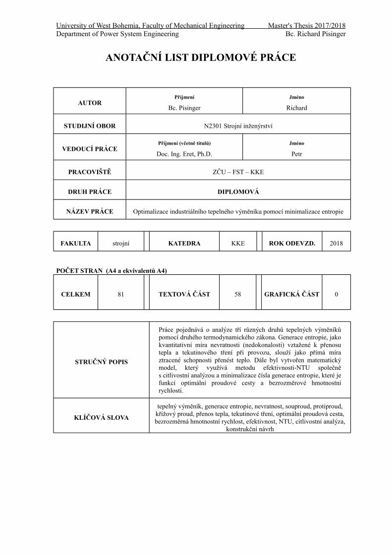
Práce pojednává o analýze tří různých druhů tepelných výměníkůpomocí druhého termodynamického zákona. Generace entropie, jakokvantitativní míra nevratnosti (nedokonalosti) vztažené k přenosutepla a tekutinového tření při provozu, slouží jako přímá míraztracené schopnosti přenést teplo. Dále byl vytvořen matematickýmodel, který využívá metodu efektivnosti-NTU společněs citlivostní analýzou a minimalizace čísla generace entropie, které jefunkcí optimální proudové cesty a bezrozměrové hmotnostnírychlosti.

KLÍČOVÁ SLOVA

tepelný výměník, generace entropie, nevratnost, souproud, protiproud,křížový proud, přenos tepla, tekutinové tření, optimální proudová cesta,bezrozměrná hmotnostní rychlost, efektivnost, NTU, citlivostní analýza,

konstrukční návrh


SUMMARY OF DIPLOMA SHEET

AUTHORSurname

Bc. Pisinger

Name

Richard

FIELD OF STUDY Design of Power Machines and Equipment

SUPERVISORSurname (Inclusive of Degrees)

Doc. Ing. Eret, Ph.D.

Name

Petr

INSTITUTION ZČU – FST – KKE

TYPE OF WORK DIPLOMA

TITLE OF THEWORK

Optimization of an industrial heat exchanger by the minimalization of entropy

FACULTYMechanicalEngineering

DEPARTMENT KKE SUBMITTED IN 2018

NUMBER OF PAGES (A4 and eq. A4)

TOTAL 81 TEXT PART 58GRAPHICAL

PART 0

BRIEF DESCRIPTION

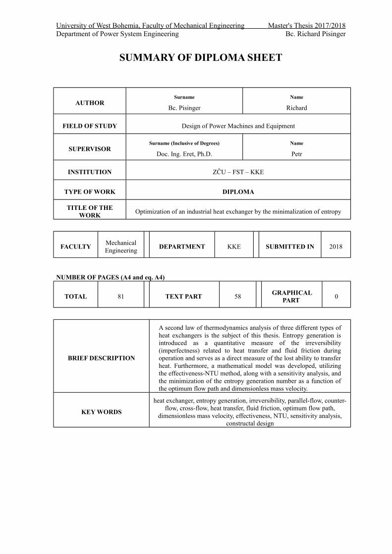
A second law of thermodynamics analysis of three different types ofheat exchangers is the subject of this thesis. Entropy generation isintroduced as a quantitative measure of the irreversibility(imperfectness) related to heat transfer and fluid friction duringoperation and serves as a direct measure of the lost ability to transferheat. Furthermore, a mathematical model was developed, utilizingthe effectiveness-NTU method, along with a sensitivity analysis, andthe minimization of the entropy generation number as a function ofthe optimum flow path and dimensionless mass velocity.

KEY WORDS

heat exchanger, entropy generation, irreversibility, parallel-flow, counter-flow, cross-flow, heat transfer, fluid friction, optimum flow path,

dimensionless mass velocity, effectiveness, NTU, sensitivity analysis,constructal design


Table of ContentsIntroduction..........................................................................................................................17

1 Overview of Heat Exchangers...........................................................................................18

1.1 Classification of heat exchangers according to fluid flow direction.........................18

1.1.1 Parallel and counter-flow...................................................................................18

1.1.2 Cross-flow heat exchangers...............................................................................22

1.1.3 Shell-and-tube heat exchangers.........................................................................24

1.1.4 Plate heat exchangers.........................................................................................27

2 Entropy and its significance..............................................................................................30

2.1 Entropy balance.........................................................................................................31

2.2 Entropy generation....................................................................................................33

2.3 Entropy Generation Minimization.............................................................................36

3 Developing the mathematical model.................................................................................37

3.1 Effectiveness-NTU Method.......................................................................................37

3.2 Sensitivity analysis of the mathematical model.........................................................51

3.3 Graphs and results.....................................................................................................57

4 Guidelines for an optimized design of a heat exchanger...................................................64

4.1 Empirical equations...................................................................................................64

4.2 Design constraints......................................................................................................67

4.2.1 Heat transfer area design constraint...................................................................68

4.2.2 Practical application of the heat transfer area design constraint........................68

5 Conclusion.........................................................................................................................72

References............................................................................................................................74

A Charts................................................................................................................................75

A.1 Effectiveness-NTU charts.........................................................................................78

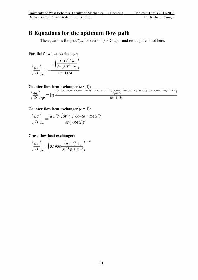
B Equations for the optimum flow path...............................................................................81


Table of FiguresFigure 1: A parallel-flow heat exchanger [2]........................................................................18

Figure 2: A counter-flow heat exchanger [2]........................................................................19

Figure 3: Overall heat transfer through a plane wall [4]......................................................20

Figure 4: Schematic of a double-pipe heat exchanger [4]....................................................20

Figure 5: Thermal-resistance network for overall heat transfer for a double-pipe heat exchanger [4]........................................................................................................................20

Figure 6: A detailed diagram of the parallel and counter-flow heat exchangers [5]............21

Figure 7: A detailed diagram of the cross-flow heat exchanger [5].....................................22

Figure 8: Cross-flow heat exchanger – unmixed and mixed flow [2]..................................22

Figure 9: Cross-flow heat exchanger pg 521 [4]..................................................................23

Figure 10: Correction factor for a single-pass cross-flow heat exchanger with both fluids unmixed [4]..........................................................................................................................24

Figure 11: Correction factor for a single-pass cross-flow heat exchanger with one fluid mixed and the other unmixed [4].........................................................................................24

Figure 12: Schematic of a shell-and-tube heat exchanger (one-shell pass and one-tube pass)[2].........................................................................................................................................24

Figure 13: Multi-pass flow arrangements in shell-and-tube heat exchangers [2]................25

Figure 14: Types of baffles used in shell-and-tube exchangers [7]......................................26

Figure 15: Correction-factor plot for exchanger with one shell pass and two, four, or any multiple of tube passes [4]....................................................................................................27

Figure 16: Correction-factor plot for exchanger with two shell passes and four, eight, or any multiple of tube passes [4].............................................................................................27

Figure 17: Gasketed plate-and-frame heat exchanger [8]....................................................28

Figure 18: Plates showing gaskets around the ports [8].......................................................28

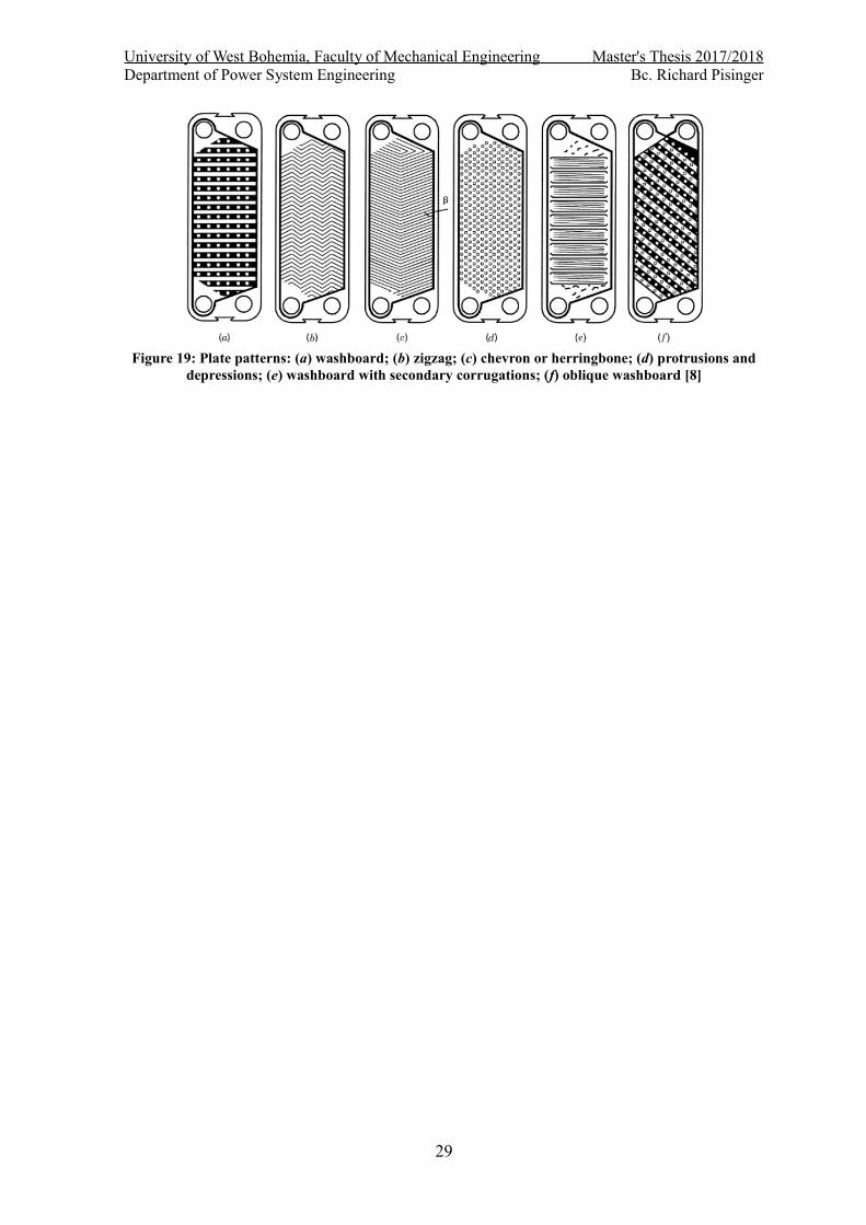
Figure 19: Plate patterns: (a) washboard; (b) zigzag; (c) chevron or herringbone; (d) protrusions and depressions; (e) washboard with secondary corrugations; (f) oblique washboard [8].......................................................................................................................29

Figure 20: Number of micro-states for each macro-state.....................................................31

Figure 21: Energy and entropy balances of a system...........................................................32

Figure 22: Mechanism of entropy transfer for a general system..........................................34

Figure 23: Entropy, heat, and mass transfer for a control volume (CV)..............................35

Figure 24: Outlet and inlet points of a heat exchanger.........................................................37

Figure 25: A case where the hot fluid has the minimum heat capacity rate (L) and a case where the cold fluid has the minimum heat capacity rate (R)..............................................38

Figure 26: Effectiveness for heat exchangers.......................................................................41

Figure 27: Comparison of the effectiveness of three heat exchangers for two different capacity ratios.......................................................................................................................42

Figure 28: Comparison of the effectiveness of three heat exchangers for two different


capacity ratios and small NTU numbers..............................................................................42

Figure 29: Effectiveness as a relation of NTU for c = 0 for all heat exchangers.................43

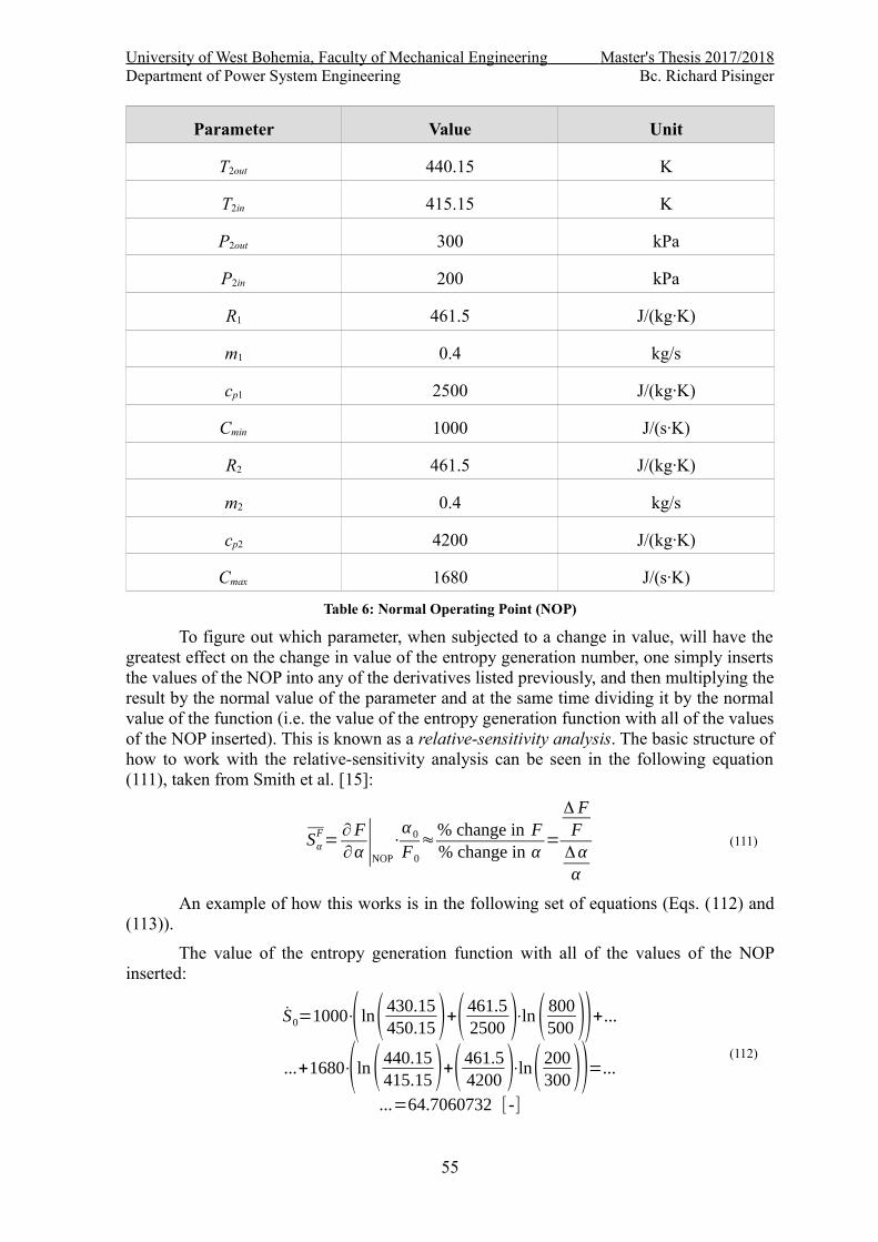
Figure 30: Relative-sensitivity analysis for the entropy generation function......................56

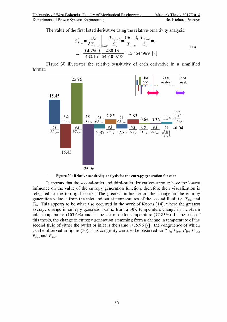
Figure 31: Variation between the optimum flow path length and the dimensionless mass velocity for all of the heat exchangers with c = 0.595238095238095.................................57

Figure 32: Variation between the minimum entropy generation number and the optimum flow path length for all of the heat exchangers with c = 0.595238095238095....................58

Figure 33: Variation between the optimum flow path length and the dimensionless mass velocity for all of the heat exchangers with c = 1................................................................58

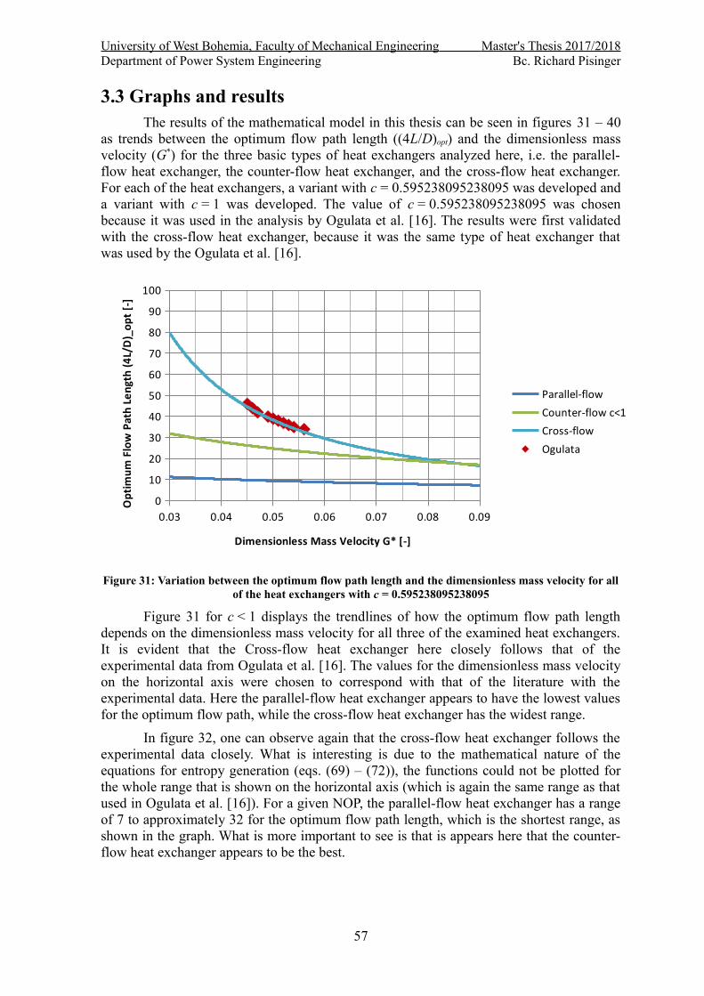
Figure 34: Variation between the minimum entropy generation number and the optimum flow path length for all of the heat exchangers with c = 1...................................................59

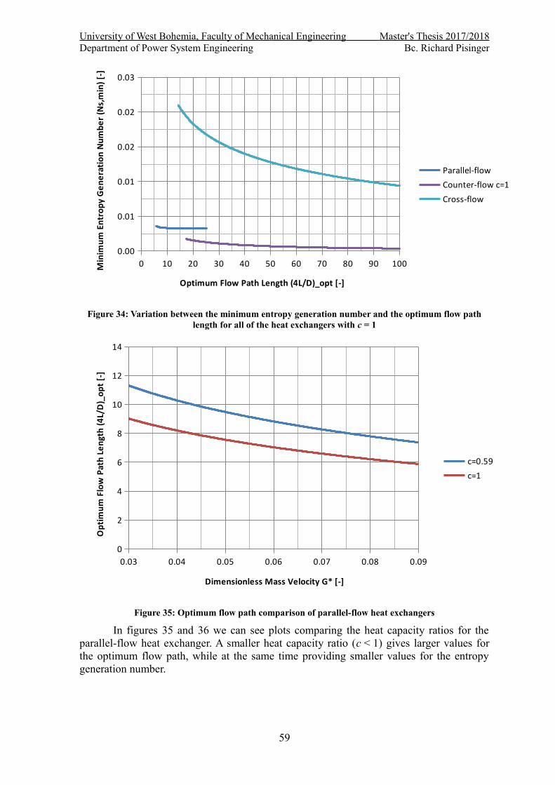
Figure 35: Optimum flow path comparison of parallel-flow heat exchangers.....................59

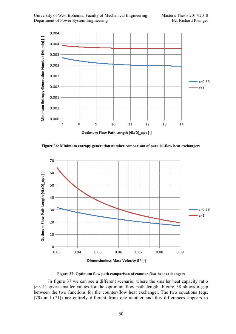
Figure 36: Minimum entropy generation number comparison of parallel-flow heat exchangers............................................................................................................................60

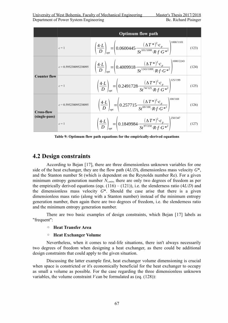
Figure 37: Optimum flow path comparison of counter-flow heat exchangers.....................60

Figure 38: Minimum entropy generation number comparison of counter-flow heat exchangers............................................................................................................................61

Figure 39: Optimum flow path comparison of cross-flow heat exchangers........................61

Figure 40: Minimum entropy generation number comparison of cross-flow heat exchangers..............................................................................................................................................62

Figure 41: Plots of the comparison between the original ε-NTU relation (blue) and the empirically-derived approximations (red)............................................................................65

Figure 42: Number of entropy generation units per side, as a function of (L/rh), g, and NRe[17].......................................................................................................................................68

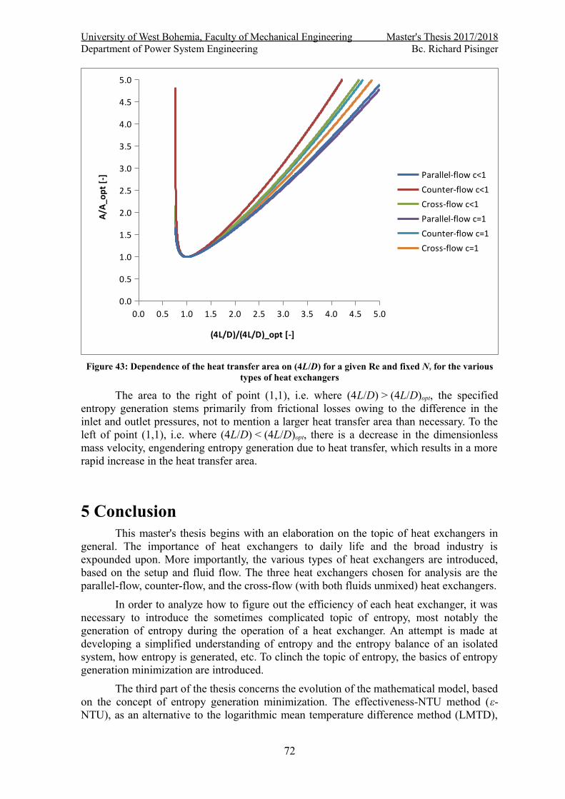
Figure 43: Dependence of the heat transfer area on (4L/D) for a given Re and fixed Ns for the various types of heat exchangers....................................................................................72

Figure 44: Variation between the optimum flow path length and the dimensionless mass velocity (L) and variation between the minimum entropy generation number and the optimum flow path length (R) for a parallel-flow heat exchanger (c = 0.595238095238095)..............................................................................................................................................75

Figure 45: Variation between the optimum flow path length and the dimensionless mass velocity (L) and variation between the minimum entropy generation number and the optimum flow path length (R) for a parallel-flow heat exchanger (c = 1)...........................75

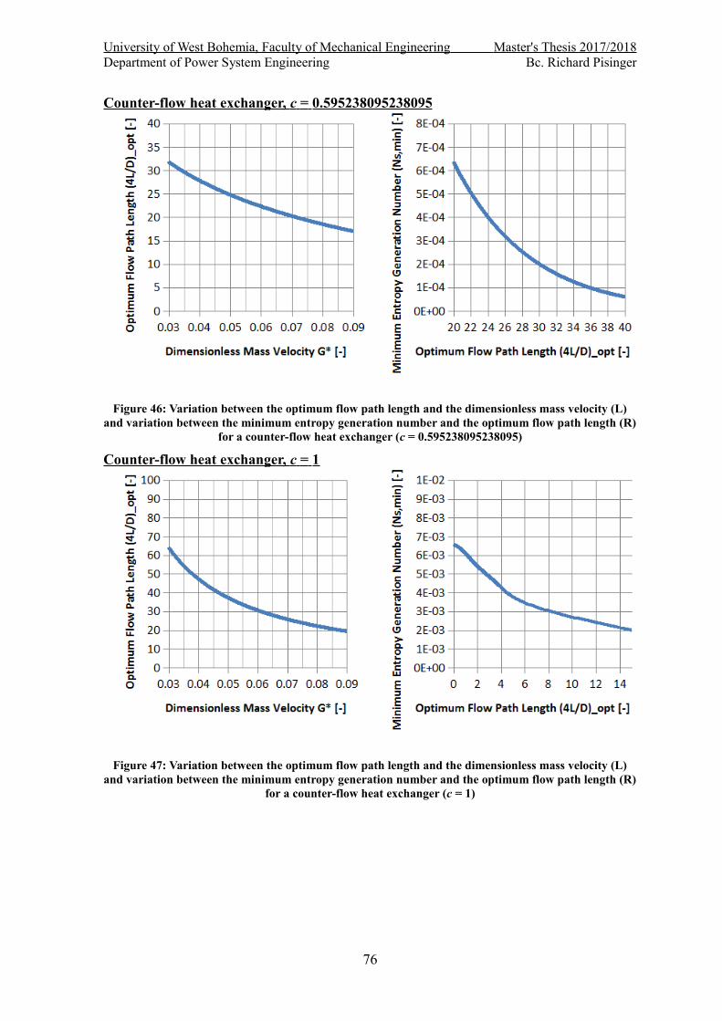
Figure 46: Variation between the optimum flow path length and the dimensionless mass velocity (L) and variation between the minimum entropy generation number and the optimum flow path length (R) for a counter-flow heat exchanger (c = 0.595238095238095)..............................................................................................................................................76

Figure 47: Variation between the optimum flow path length and the dimensionless mass velocity (L) and variation between the minimum entropy generation number and the optimum flow path length (R) for a counter-flow heat exchanger (c = 1)...........................76

Figure 48: Variation between the optimum flow path length and the dimensionless mass velocity (L) and variation between the minimum entropy generation number and the optimum flow path length (R) for a cross-flow heat exchanger (c = 0.595238095238095)77


Figure 49: Variation between the optimum flow path length and the dimensionless mass velocity (L) and variation between the minimum entropy generation number and the optimum flow path length (R) for a cross-flow heat exchanger (c = 1)...............................77

Figure 50: Variation between the effectiveness and the number of transfer units for a parallel-flow heat exchanger................................................................................................78

Figure 51: Variation between the effectiveness and the number of transfer units for a counter-flow heat exchanger................................................................................................78

Figure 52: Variation between the effectiveness and the number of transfer units for a cross-flow heat exchanger..............................................................................................................79

Figure 53: Variation between the effectiveness and the number of transfer units for all of the heat exchangers with c = 0.595238095238095..............................................................79

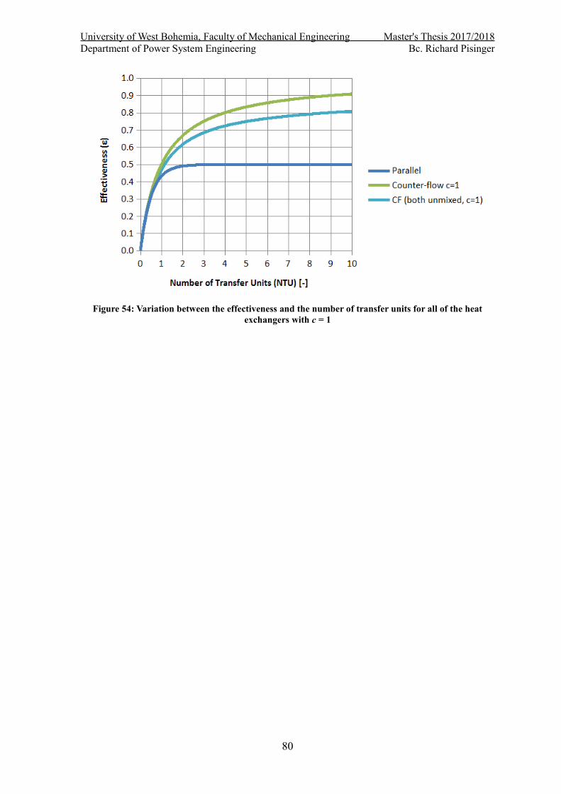
Figure 54: Variation between the effectiveness and the number of transfer units for all of the heat exchangers with c = 1.............................................................................................80


Table of TablesTable 1: Effectiveness relations for heat exchangers [13]....................................................40

Table 2: NTU relations for heat exchangers [13].................................................................44

Table 3: Modified entropy generation equations..................................................................49

Table 4: Modified entropy generation equations..................................................................50

Table 5: Table of derivatives for the sensitivity analysis......................................................54

Table 6: Normal Operating Point (NOP)..............................................................................55

Table 7: X and Y coefficients of the empirically-derived equations....................................64

Table 8: Entropy generation equations for the empirically-derived equations.....................66

Table 9: Optimum flow path equations for the empirically-derived equations....................67

Table 10: Optimum flow path equations for the empirically-derived equations..................69

Table 11: Minimum heat transfer area equations for the empirically-derived equations.....70

Table 12: Optimum dimensionless mass velocity equations for the empirically-derived equations...............................................................................................................................71


List of Abbreviations• ε-NTU – effectiveness-NTU method

• EGM – entropy generation minimization

• LMTD – logarithmic mean temperature difference

• NTU – number of transfer units


List of Frequently Used Symbols

Symbol Unit Property

A [m2]Surface area through which convection heat transfer takes place

Ai [m2]Surface area of the inner wall through which convection heat transfer takes place

Ao [m2]Surface area of the outer wall through which convection heat transfer takes place

As [m2]Heat transfer surface area of the heat exchanger

c [-] Heat capacity ratio

Cc [J∙kg-1∙K-1]Heat capacity rate of the “cold” fluid

Ch [J∙kg-1∙K-1]Heat capacity rate of the “hot”fluid

Cmax [J∙kg-1∙K-1]The larger of the two heat capacities of a heat exchanger

Cmin [J∙kg-1∙K-1]The smaller of the two heat capacities of a heat exchanger

Cp [J∙kg-1∙K-1] Heat capacity

D [m] Diameter

F [-] Correction factor

f [-] Friction

G [kg∙m-2∙s-1] Mass velocity

G* [-] Dimensionless mass velocity

h1 [W·m-2·K-1]Convection heat transfer coefficient of fluid 1

h2 [W·m-2·K-1]Convection heat transfer coefficient of fluid 2

k [W·m-2·K-1]Thermal conductivity of a material

k J∙K-1 Boltzmann constant

L [m] Length

m [kg] Mass

m [kg∙s-1] Mass transfer rate

me [kg] Exit mass



mi [kg] Inlet mass

NTU [-] Number of heat transfer units

Nu [-] Nusselt number

P [-] Temperature Ratio

P1,in [Pa] Inlet pressure of fluid 1

P1,out [Pa] Outlet pressure of fluid 1

P2,in [Pa] Inlet pressure of fluid 2

P2,out [Pa] Outlet pressure of fluid 2

pc,in [Pa]Inlet pressure of the “cold” fluid

pc,out [Pa]Outlet pressure of the “cold” fluid

ph,in [Pa]Inlet pressure of the “hot” fluid

ph,out [Pa]Outlet pressure of the “hot” fluid

Pr [-] Prandtl number

q [J] Heat transfer

Q [J] Heat transfer

Q [J∙s-1] Heat transfer rate

Qmax [J∙s-1] Max heat transfer rate

R1 [J∙kg-1∙K-1] Ideal gas constant

R2 [J∙kg-1∙K-1] Ideal gas constant

Re [-] Reynolds number

ri [m] Radius of inner wall

ro [m] Radius of outer wall

S [m2] Surface area

S [J∙K-1] Entropy

s [J∙K-1] Entropy

se [J∙K-1] Exit entropy

Sgen [J∙K-1] Entropy generation

si [J∙K-1] Inlet entropy

St [-] Stanton number

T1,in [K] Inlet temperature of fluid 1

T1,out [K] Outlet temperature of fluid 1

T2,in [K] Inlet temperature of fluid 2



T2,out [K] Outlet temperature of fluid 2

Tc,in [K]Inlet temperature of the “cold” fluid

Tc,out [K]Outlet temperature of the “cold” fluid

Th,in [K]Inlet temperature of the “hot” fluid

Th,out [K]Outlet temperature of the “hot” fluid

U [W·m-2·K-1]Overall heat transfer coefficient

V [m3] Volume of the system

W [-] Number of micro-states

α1 [m2∙s-1] Thermal diffusivity of fluid 1

α2 [m2∙s-1] Thermal diffusivity of fluid 2

δ [m] Wall thickness

ΔSCV [J∙K-1] Entropy for a control volume

ΔTlm [K]Logarithmic mean temperature difference

ΔTlm,CF [K]Logarithmic mean temperature difference of a counter-flow heat exchanger

ε [-] Effectiveness

λ [W∙m-1∙K-1] Thermal conductivity

ρ [kg∙m-3] Density


IntroductionA heat exchanger can be thought of as any device, the primary purpose of which is

to transfer heat from a fluid with a higher amount of thermal energy (enthalpy) to a secondfluid, which has a lower amount of thermal energy. These two fluids are prevented frommixing by a solid wall, which is one of the primary components of the heat exchanger.Examples of heat exchangers are quite commonplace in the everyday life of the individual.An elementary example of a heat exchanger is a kettle, which is used to transfer heat froma heating element into the water, the continuing transferring of which eventually results inthe boiling of said water. Another common example is a refrigerator, the basic principle ofwhich involves transferring heat from the stored victuals and expelling the heat into thesurrounding area, with the aid of electrical energy to power the fridge.

A more refined example of where heat exchangers can be used is in power plantsthat generate electricity using steam turbines. At the end of a turbine, when the steam hasexpanded such and expended most of its usable energy to the generator (for generatingelectricity), it still has enough enthalpy to be useful for heat regeneration. This process isdone via heat exchangers, where some of the heat from the steam (before it reaches thecondenser) is taken and used to heat the condensate in a process called “regeneration”,which ultimately increases the thermal efficiency of the power plant. With regard to powerplants, a visible example of a heat exchanger is a cooling tower, notably a wet coolingtower, where sprinklers in the cooling tower release liquid water onto hot tubes containingwater, which is holding the disposable thermal energy of the power plant. The water thenevaporates off of the outside of the tubes and into the atmosphere, resulting in a usuallyvisible cloud stemming from the tower.

In a heat exchanger, there are usually two different kinds of heat transfer –convection in each fluid and conduction through the wall, which is keeping the two fluidsfrom mixing. However, when working with heat exchangers, these processes are usuallycombined into an overall heat transfer coefficient. The value of this coefficient can varydepending on the position along the wall separating the two fluids.

17


1 Overview of Heat ExchangersThe classification of heat exchangers can be either based on how the mediums flow

with respect to one another or according to how they are built. An example of the formerincludes heat exchangers with counter-current flow, where the two fluids flow in oppositedirections to each other, but in a parallel manner. Another example is a heat exchanger withcocurrent or parallel flow, which is the same as the previous example but the two fluidsnow flow in the same direction. Cross-flow heat exchangers have the media flowperpendicular to one another. A cross-flow/counter-flow heat exchanger is a hybrid of thepreviously mentioned heat exchangers. The first two types of heat exchangers can be seenin figures 1 and 2.

As mentioned, heat exchangers can be classified according to how they areconstructed. From here they can be further classified into the following categories –recuperative and regenerative heat exchangers. Recuperative heat exchangers have a wallseparating the fluids flowing through the heat exchanger, which have different flow pathsand exchange their heat through this separating barrier. Regenerative heat exchangers onthe other hand involves a single flow path, through which the hot and cold mediumsalternatively flow. [1]

1.1 Classification of heat exchangers according to fluid flow direction

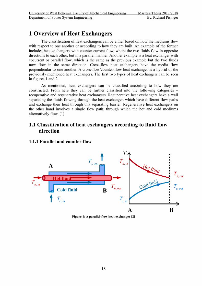
1.1.1 Parallel and counter-flow

Figure 1: A parallel-flow heat exchanger [2]

18

A

B

Tc, out

Th, in

Tc, in

Th, in

Tc, in

Th, out

Tc, out

Th, out

A B

T

Hot fluid

Cold fluidHot fluid

Cold fluid


Figure 2: A counter-flow heat exchanger [2]

The prevailing types of fluid flow arrangement within heat exchangers are thosewith parallel or counter-flow. Regarding how the heat transfer process works pertaining toboth of these arrangements, both conduction and convection are involved. The heat transferprocess starts with the hot fluid, where the fluid starts to transfer its heat by convection tothe tubular wall, whereby the heat is conducted through the wall to the side of the wall,which is in contact with the second, colder fluid. The heat is then transferred by the processof convection to this second fluid. Nevertheless, this process of heat transfer is not constantalong the entire length of the tube within the heat exchanger, for the temperature differencebetween the two fluids varies along this length, thereby affecting the rate of heat transfer.Figure 3 shows an example of how this works.

A counter-flow heat exchanger is generally preferred to that of a heat exchangerwith parallel-flow due to some of the advantages of the former to that of the latter. One ofthe advantages lies in the fact that the outlet temperature of the cold fluid can come closeto, or be lower than, that of the inlet temperature of the hot fluid. Another advantage is thatthe more uniform temperature difference between the two fluids provides for a moreuniform rate of heat transfer along the length of the tubular contact between the two fluidswithin the heat exchanger, which has the added advantage of mitigating the thermalstresses of the heat exchanger. These advantages yield greater heat recovery and to a morecompact heat exchanger, regarding the counter-flow design.

Adding to the advantages of the counter-flow heat exchanger, there are twosignificant disadvantages of the parallel-flow design. One of the disadvantages isevidenced in the considerable temperature difference between the starting and endingpoints of the heat exchanger. This can lead to unwarranted large thermal stresses,contributing to possible material failure. A second point to make is that at the end of theheat exchanger, the outlet temperature of the cold fluid can never be lesser than that of theinlet temperature of the hot fluid, which however, can be considered an advantage if thegoal is to have both of the outlet temperatures to be at around the same temperature [3].

Notwithstanding, there can be cases where a parallel-flow design can beadvantageous. Besides cases where one would require the outlet temperatures of the fluidsto be similar, should one require fast heat transfer, then the parallel-flow design should besuitable, as at the start of the heat exchanger, there is an enormous temperature difference,which is more easily achieved with this kind of design, contrary to the counter-flow type.Another case arises when one of the fluids is undergoing a phase change, during which the

19

A

B

Tc, in

Th, in

Tc, out

Th, in

Tc, in

Th, out

Tc, out

Th, out

A B

THot fluid

Cold fluidHot fluid

Cold fluid


temperature for this fluid does not change during its phase change, which means that eitherof the two designs, the parallel or counter-flow, can be utilized to no disadvantage [1].

Figure 3: Overall heat transfer through a plane wall [4]

When it comes to calculating the heat transfer through a planar surface, thefollowing calculations apply (eqs. (1) and (2)):

Q=k⋅S⋅ΔT S=1

1α1

+δλ+

1α2

⋅S⋅ΔT S(1)

k=( 1α1

+δλ+

1α2 )

−1

(2)

where S is the area, δ is the thickness, λ, α1, α2, k is the heat transfer coefficient, and ΔTS isthe mean temperature difference. Figure 4 shows an example of the heat transfer process ina double-pipe (parallel-flow) heat exchanger.

Figure 4: Schematic of a double-pipe heat exchanger [4]

Figure 5: Thermal-resistance network for overall heat transfer for a double-pipe heat exchanger [4]

When one goes about calculating the heat transfer through a tubular wall, the

20

TA

TB

T1

T2

h1

h2

q

Fluid A

Fluid B TA

T1

T2

TB

1h1⋅A

Δ xk⋅A

1h2⋅A

q

TA

Ti

To

TB

1h1⋅A i

lnror i

2⋅π⋅k⋅L

1h2⋅Ao

q

FLUID A

FLUID B


following calculations apply (eqs. (3) and (4)):

Q=k⋅S⋅ΔT S=1

1α1

⋅R2

R1

+R2

λ⋅ln

R2

R1

+1α2

⋅2⋅π⋅R2⋅L⋅ΔT S(3)

k=( 1α1

⋅R2

R1

+R2

λ⋅ln

R2

R1

+1α2)−1

(4)

where L is the length, R1 is the inner wall radius, R2 is the outer wall radius, λ, α1, α2, k isthe heat transfer coefficient, and ΔTS is the mean temperature difference.

Figure 6: A detailed diagram of the parallel and counter-flow heat exchangers [5]

Figure 6 shows a side-by-side visual comparison of the LMTD diagrams forillustrative purposes. The calculations for the log mean temperature difference are the samefor both the parallel and counter-flow heat exchangers, as can be seen in eqs. (5) – (8):

ΔT=ΔT '⋅e−k⋅x , k=? (5)

ΔT ' '=ΔT '⋅e−k⋅L⇒ −k⋅L=ln ΔT ''

ΔT '⇒ k=−

1L⋅ln ΔT ''

ΔT '(6)

ΔT=ΔT '⋅exL⋅ln ΔT ''

ΔT ' (7)

ΔT S=1L∫0

L

ΔT⋅d x=ΔT 'L

⋅∫0

L

exL⋅ln ΔT ''

ΔT '⋅d x=

1L⋅ΔT '⋅e

xL⋅ln Δ T ''

ΔT ' |0

L

1L⋅ln

ΔT ''ΔT '

=...

...=ΔT '⋅(e ln

ΔT ''ΔT ' −1)

lnΔT ''ΔT '

=

ΔT '⋅(ΔT ''ΔT '

−1)ln

ΔT ''ΔT '

=ΔT ''−ΔT '

lnΔT ''ΔT '

=ΔT '−ΔT ''

lnΔT 'ΔT ''

(8)

21


1.1.2 Cross-flow heat exchangers

Figure 7: A detailed diagram of the cross-flow heat exchanger [5]

When a heat exchanger is of the cross-flow type, the two fluids in the heatexchanger are perpendicular to each other, as seen in figure 7. One of the fluids flowsthrough a tubular structure, while the other fluid flows around this structure at a 90-degreeangle. This type of heat exchanger is most often utilized in situations where one of the fluidundergoes a phase change. An example can be found in a steam-driven power plant, in thecondenser. The condenser is comprised of tubes, through which the coolant flows through,thereby absorbing the heat from the steam (which has just left the turbine and entered thecondenser), which is flowing around the tubes. The steam is then condensed into liquidwater [6].

Figure 8: Cross-flow heat exchanger – unmixed and mixed flow [2]

Cross-flow heat exchangers can also be divided into two subgroups – mixed andunmixed flow, as can be seen in figure 8. Unmixed flow is where neither of the two fluidsare mixed, as in the previous example with the steam condenser. Mixed cross-flow heatexchangers are simpler and have one of the fluids, namely that of the fluid flowing throughthe tubular structure, stay unmixed and the other fluid, also known as the cross-flow,become mixed (such as the surrounding air) [2].

These types of heat exchangers, i.e. of the cross-flow type, are most often utilizedin cooling applications or in air/gas heating. An example of the mixed type of cross-flowheat exchanger can be seen when it comes to radiators in an apartment, the heated waterflows through the tubes of the radiator (unmixed), whereas the air around the radiator ismixed, e.g. with various odors and potential pollutants.

22

Cross-flow (unmixed)

Cross-flow (mixed)

Tube-flow (unmixed)

Tube-flow (unmixed)

T1''

T2''T

2'

T1'


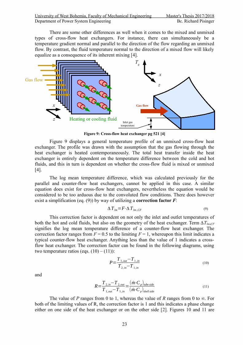
There are some other differences as well when it comes to the mixed and unmixedtypes of cross-flow heat exchangers. For instance, there can simultaneously be atemperature gradient normal and parallel to the direction of the flow regarding an unmixedflow. By contrast, the fluid temperature normal to the direction of a mixed flow will likelyequalize as a consequence of its inherent mixing [4].

Figure 9: Cross-flow heat exchanger pg 521 [4]

Figure 9 displays a general temperature profile of an unmixed cross-flow heatexchanger. The profile was drawn with the assumption that the gas flowing through theheat exchanger is heated contemporaneously. The total heat transfer inside the heatexchanger is entirely dependent on the temperature difference between the cold and hotfluids, and this in turn is dependent on whether the cross-flow fluid is mixed or unmixed[4].

The log mean temperature difference, which was calculated previously for theparallel and counter-flow heat exchangers, cannot be applied in this case. A similarequation does exist for cross-flow heat exchangers, nevertheless the equation would beconsidered to be too arduous due to the convoluted flow conditions. There does howeverexist a simplification (eq. (9)) by way of utilizing a correction factor F:

ΔT lm=F⋅ΔT lm ,CF (9)

This correction factor is dependent on not only the inlet and outlet temperatures ofboth the hot and cold fluids, but also on the geometry of the heat exchanger. Term ΔTlm,CF

signifies the log mean temperature difference of a counter-flow heat exchanger. Thecorrection factor ranges from F = 0.5 to the limiting F = 1, whereupon this limit indicates atypical counter-flow heat exchanger. Anything less than the value of 1 indicates a cross-flow heat exchanger. The correction factor can be found in the following diagrams, usingtwo temperature ratios (eqs. (10) – (11)):

P=T 1 ,out−T 1 , in

T 2 , in−T 1 , in

(10)

and

R=T 2 , in−T 2 ,out

T 1 ,out−T 1 , in

=(m⋅C p)tube side(m⋅C p)shell side

(11)

The value of P ranges from 0 to 1, whereas the value of R ranges from 0 to ∞. Forboth of the limiting values of R, the correction factor is 1 and this indicates a phase changeeither on one side of the heat exchanger or on the other side [2]. Figures 10 and 11 are

23

Gas flow

Heating or cooling fluid

x

z

Tg

x

z

Inlet gas temperature

Gas flow


diagrams showing the correction factor for two different types of heat exchangers.

Figure 10: Correction factor for a single-pass cross-flow heat exchanger with both fluids unmixed [4]

Figure 11: Correction factor for a single-pass cross-flow heat exchanger with one fluid mixed and theother unmixed [4]

1.1.3 Shell-and-tube heat exchangers

Figure 12: Schematic of a shell-and-tube heat exchanger (one-shell pass and one-tube pass) [2]

24

Tube outlet

Shell inlet

Rear-end header

Tubes ShellShell outlet

Tube inlet

Front-end header

Baffles


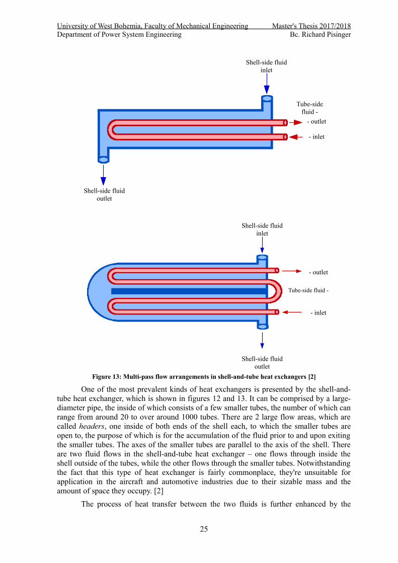
Figure 13: Multi-pass flow arrangements in shell-and-tube heat exchangers [2]

One of the most prevalent kinds of heat exchangers is presented by the shell-and-tube heat exchanger, which is shown in figures 12 and 13. It can be comprised by a large-diameter pipe, the inside of which consists of a few smaller tubes, the number of which canrange from around 20 to over around 1000 tubes. There are 2 large flow areas, which arecalled headers, one inside of both ends of the shell each, to which the smaller tubes areopen to, the purpose of which is for the accumulation of the fluid prior to and upon exitingthe smaller tubes. The axes of the smaller tubes are parallel to the axis of the shell. Thereare two fluid flows in the shell-and-tube heat exchanger – one flows through inside theshell outside of the tubes, while the other flows through the smaller tubes. Notwithstandingthe fact that this type of heat exchanger is fairly commonplace, they're unsuitable forapplication in the aircraft and automotive industries due to their sizable mass and theamount of space they occupy. [2]

The process of heat transfer between the two fluids is further enhanced by the

25

Shell-side fluid inlet

Shell-side fluid outlet

Tube-side fluid -

- outlet

- inlet

Shell-side fluid inlet

Shell-side fluid outlet

Tube-side fluid -

- inlet

- outlet


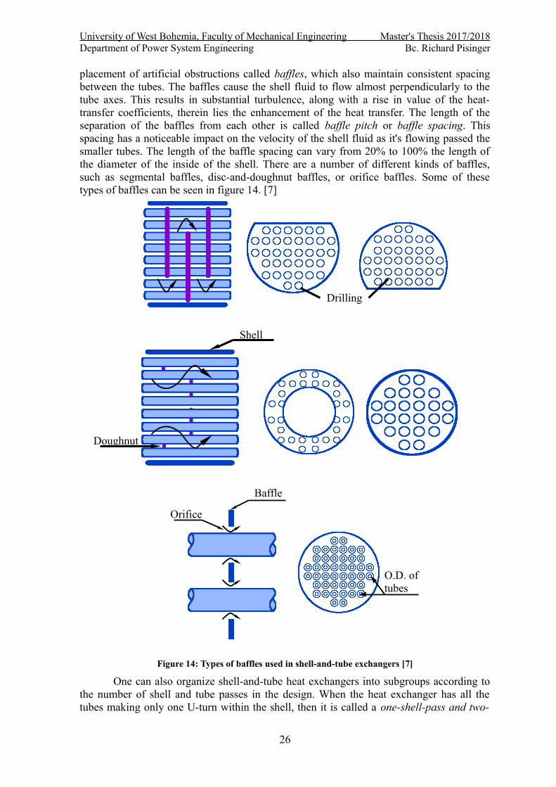
placement of artificial obstructions called baffles, which also maintain consistent spacingbetween the tubes. The baffles cause the shell fluid to flow almost perpendicularly to thetube axes. This results in substantial turbulence, along with a rise in value of the heat-transfer coefficients, therein lies the enhancement of the heat transfer. The length of theseparation of the baffles from each other is called baffle pitch or baffle spacing. Thisspacing has a noticeable impact on the velocity of the shell fluid as it's flowing passed thesmaller tubes. The length of the baffle spacing can vary from 20% to 100% the length ofthe diameter of the inside of the shell. There are a number of different kinds of baffles,such as segmental baffles, disc-and-doughnut baffles, or orifice baffles. Some of thesetypes of baffles can be seen in figure 14. [7]

Figure 14: Types of baffles used in shell-and-tube exchangers [7]

One can also organize shell-and-tube heat exchangers into subgroups according tothe number of shell and tube passes in the design. When the heat exchanger has all thetubes making only one U-turn within the shell, then it is called a one-shell-pass and two-

26

Drilling

Doughnut

Shell

Baffle

Orifice

O.D. of tubes


tube-passes heat exchanger. Should it have two passes, then it's known as a two-shell-passes and four-tube-passes heat exchanger. As for the cross-flow heat exchanger, figures15 and 16 are diagrams showing the correction factor for two different types of shell-and-tube heat exchangers. [4]

Figure 15: Correction-factor plot for exchanger with one shell pass and two, four, or any multiple oftube passes [4]

Figure 16: Correction-factor plot for exchanger with two shell passes and four, eight, or any multiple oftube passes [4]

1.1.4 Plate heat exchangers

This type of heat exchanger is comprised by a series of thin plates, which are eithersmooth or corrugated and there's a small space between each plate. These plates have verybroad surface areas and encompass narrow fluid passages; these passages alternatebetween “hot” and “cold” fluids, so that each “cold” fluid is surrounded by two “hot”fluids and vice-versa.

Today's technology, concerning the usage of gaskets and the process of brazing, hasadvanced far enough so as to make the application of this type of heat exchanger morefeasible. Larger heat exchangers of this type are known as the plate-and-frame heatexchanger and can be commonly found in HVAC (Heating Ventilation and AirConditioning) applications. They can be applied either in an open-loop or closed-loop (e.g.refrigeration) setting. The advantage with an open-loop is that this kind of heat exchangercan be easily disassembled, cleaned, and maintained.

27


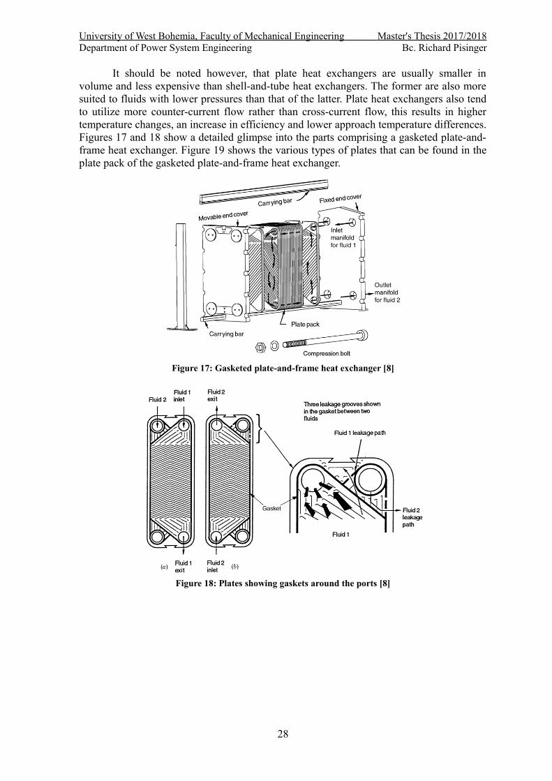
It should be noted however, that plate heat exchangers are usually smaller involume and less expensive than shell-and-tube heat exchangers. The former are also moresuited to fluids with lower pressures than that of the latter. Plate heat exchangers also tendto utilize more counter-current flow rather than cross-current flow, this results in highertemperature changes, an increase in efficiency and lower approach temperature differences.Figures 17 and 18 show a detailed glimpse into the parts comprising a gasketed plate-and-frame heat exchanger. Figure 19 shows the various types of plates that can be found in theplate pack of the gasketed plate-and-frame heat exchanger.

Figure 17: Gasketed plate-and-frame heat exchanger [8]

Figure 18: Plates showing gaskets around the ports [8]

28


Figure 19: Plate patterns: (a) washboard; (b) zigzag; (c) chevron or herringbone; (d) protrusions anddepressions; (e) washboard with secondary corrugations; (f) oblique washboard [8]

29


2 Entropy and its significanceThe definition of entropy is directly related to the Second Law of Thermodynamics,

i.e. that any spontaneous process increases the disorder of the universe. One can say thatthe change of entropy is embodied in all natural affairs as the driving motive. Naturalevents are irreversible, ergo every single of them alters the universe from its previous state.One can characterize an irreversible process as that being a passage from a less probable toa more probable state of the system, or from a less stable to a more stable state of thesystem, all the while being of a spontaneous nature, i.e. it starts and proceeds without anyexternal stimuli.

Entropy is a direct measure of each energy configurations probability, it's ameasurement of how energy is spread out in the system.

According to Klein [9], the following are some general statements that serve todescribe the characteristics of the entropy of a state:

a) Entropy is a universal measure of the "disorder" in the mass points of a system.

b) Entropy is a universal measure of the irreversibility of a state and is itscriterion as well.

c) Entropy is a universal measure of nature's preference for the state.

d) Entropy is a universal measure of the spontaneity with which a state acts whenit is free to change.

e) Entropy of a system can only grow.

f) Entropy asserts the essential one-sidedness of Nature.

g) There exists in Nature a magnitude which always changes in the same sense.

As mentioned in one of the general definitions of entropy, it can be characterized asa universal measurement of disorder. However, one can ask themselves the question as towhat exactly is this disorder? An example can be found in a case where there are two glasscups, one is filled with crushed ice, whereas the other glass is filled with liquid water. Atfirst glance, one can be easily mislead into believing that since the glass with the crushedice appears to be more disordered, that it's the substance with a higher entropy.Nonetheless, it is in fact the substance with a lower level of entropy. This is due to the factthat one requires less information to know about the positions of every molecule in thecrushed ice than with the molecules in the liquid water. In the crushed ice, aside from thevibrations of each molecule (as with all solids), the molecules are more or less in the samepositions in the lattice structure of the ice, whereas the molecules in the liquid water arefree to randomly move past each other, ergo one needs to know the positions of every exactmolecule at a specific point in time in the liquid water.

The German theoretical physicist Max Planck discovered that the entropy of a stateis entirely dependent on what he termed as the “probability” of the state. The followingformula (eq. (12)) was first devised by him.

S=k⋅logW (12)

where S is entropy [J∙K-1], W is the probability of a state [-], and k is the Boltzmannconstant, the recommended value of which is approximately 1.3807∙10−23 J∙K-1.

One can see how this definition of entropy works in another example, where there

30


are two containers of the same size and structure. One container has six different objects,while the other container has none. There is only one way one can arrive at thisconfiguration, or only one micro-state. Moving on, the next situation, or macro-state, toarrive at is where there are five different objects in the first container and one object in thesecond. There are six different configurations, or micro-states in this case, and so moreentropy than for the first macro-state. The macro-state with the highest level of entropy, i.e.three objects in the first container and three objects in the second, resulting in a total oftwenty micro-states.

This can be seen in the following equation (eq. (13)):

W=( nm)=n !

m!⋅(n−m)!(13)

where W is the number of micro-states [-], n is the number of objects in total (6 in thiscase) [-], and m is the number of objects in the second container [-]. The result can be seenin the following diagram (figure 20).

Figure 20: Number of micro-states for each macro-state

Naturally, when you have a much larger number of macro-states, the shape of theentropy distribution much less resembles a mountain and starts to resemble more of aplateau. So in the real world, it is statistically more likely for a system to incur higherentropy. This resulted in entropy being labeled as "time's arrow", which means that ifenergy acquires the opportunity to spread out, it will.

2.1 Entropy balanceHarking back to the basic definition of entropy, according to the second law of

thermodynamics, entropy can only be created, i.e. it cannot be destroyed. This means thatthe entropy of a system can either only rise or not change at all, ergo, it can never decrease.This can be easily shown in figure 21:

31

1 2 3 4 5 6 70

2

4

6

8

10

12

14

16

18

20

Number of micro-states for each macro-state

Macro-state

Num

ber

of m

icro

-sta

tes

[-]


Figure 21: Energy and entropy balances of a system

What is shown in figure 21 can also be expressed either as:

(Total

entropyentering)−(

Totalentropyleaving)+(

Totalentropy

generated)=(Change in thetotal entropyof the system)

or as equation (14):

Sin – Sout + Sgen = ΔSsystem (14)

which is known as the entropy balance. This latter formula, i.e. the entropy balance(eq. (14)), can be applied to any system irrespective of any process that it's undergoing.According to corresponding literature [10], there is a fitting description related to theentropy balance, i.e.: the entropy change of a system during a process is equal to the netentropy transfer through the system boundary and the entropy generated within the system.In contrast to energy, which can exist in many forms, entropy can only exist in one form.Therefore, it is easy to conclude that the way to determine the entropy change of a systemis to evaluate the amount of entropy at the beginning and the conclusion of a process. Thiscan be stated in equation (15):

ΔSsystem = Sfinal – Sinitial = S2 – S1 (15)

It should be stated that the entropy change of a system will be equal to zero,because entropy is a property, the value of which is immutable, unless the state of thesystem is modified. The latter equation, however, is only applicable to a system, where itsproperties are uniform. In the opposite case, the way to determine the entropy of thesystem is by way of integration (eq. (16)):

Ssystem=∫ s⋅dm=∫v

s⋅ρ⋅dV (16)

where s is the specific entropy of the process [kJ∙kg-1], m is the mass of the system [kg], ρis the density of the system [kg∙m-3], and V is the volume of the system [m3].

There are two different ways in how entropy can be transferred to or from a system.One mechanism is by heat transfer and the other is by mass flow. It can be said that it's likeenergy in this respect, with the difference being that energy can also be transferred bywork. Change in entropy occurs as entropy crosses the confines of a system; this change isa measure of the amount of entropy that is obtained or forfeited by the system. It can beconcluded that for an adiabatic closed system the entropy transfer is zero, because the onlymechanism, with which the entropy transfer of a system is realized, is heat transfer, ergo

32

System

ΔEsystemΔSsystem

Sgen ≥ 0

Ein

Sin

Eout

Sout

ΔEsystem = Ein − EoutΔSsystem = Sin − Sout + Sgen


the heat transfer to and from an adiabatic closed system is zero.

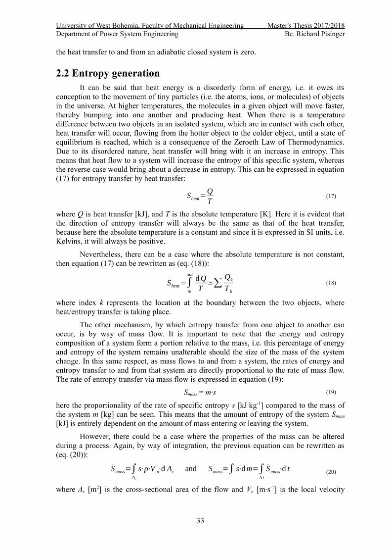
2.2 Entropy generationIt can be said that heat energy is a disorderly form of energy, i.e. it owes its

conception to the movement of tiny particles (i.e. the atoms, ions, or molecules) of objectsin the universe. At higher temperatures, the molecules in a given object will move faster,thereby bumping into one another and producing heat. When there is a temperaturedifference between two objects in an isolated system, which are in contact with each other,heat transfer will occur, flowing from the hotter object to the colder object, until a state ofequilibrium is reached, which is a consequence of the Zeroeth Law of Thermodynamics.Due to its disordered nature, heat transfer will bring with it an increase in entropy. Thismeans that heat flow to a system will increase the entropy of this specific system, whereasthe reverse case would bring about a decrease in entropy. This can be expressed in equation(17) for entropy transfer by heat transfer:

Sheat=QT

(17)

where Q is heat transfer [kJ], and T is the absolute temperature [K]. Here it is evident thatthe direction of entropy transfer will always be the same as that of the heat transfer,because here the absolute temperature is a constant and since it is expressed in SI units, i.e.Kelvins, it will always be positive.

Nevertheless, there can be a case where the absolute temperature is not constant,then equation (17) can be rewritten as (eq. (18)):

Sheat=∫in

outdQT

≃∑Qk

T k

(18)

where index k represents the location at the boundary between the two objects, whereheat/entropy transfer is taking place.

The other mechanism, by which entropy transfer from one object to another canoccur, is by way of mass flow. It is important to note that the energy and entropycomposition of a system form a portion relative to the mass, i.e. this percentage of energyand entropy of the system remains unalterable should the size of the mass of the systemchange. In this same respect, as mass flows to and from a system, the rates of energy andentropy transfer to and from that system are directly proportional to the rate of mass flow.The rate of entropy transfer via mass flow is expressed in equation (19):

Smass = m∙s (19)

here the proportionality of the rate of specific entropy s [kJ∙kg-1] compared to the mass ofthe system m [kg] can be seen. This means that the amount of entropy of the system Smass

[kJ] is entirely dependent on the amount of mass entering or leaving the system.

However, there could be a case where the properties of the mass can be alteredduring a process. Again, by way of integration, the previous equation can be rewritten as(eq. (20)):

Smass=∫A c

s⋅ρ⋅V n⋅d Ac and Smass=∫ s⋅dm=∫Δ t

Smass⋅d t (20)

where Ac [m2] is the cross-sectional area of the flow and Vn [m∙s-1] is the local velocity

33


normal to dAc.

A point of note should also be made about the distinction between energy transferand entropy transfer. Whereas energy can be transferred by both heat and work, entropycan only be transferred by heat. This means that the entropy transfer rate by way of workamounts to zero.

According to thermodynamic theory [10], irreversibilities such as friction, mixing,chemical reactions, heat transfer through a finite temperature difference, unrestrainedexpansion, nonquasi-equilibrium compression, or expansion always cause the entropy of asystem to increase, and entropy generation is a measure of the entropy created by sucheffects during a process. Nevertheless, since in order for there to be irreversible processesthere must be reversible processes. In this latter case, the entropy generation is nonexistent,and so the entropy change of a system undergoing this kind of process amounts to the samevalue as that of the entropy transfer. One can therefore conclude that the entropy balancerelation will correspond with the energy balance relation, i.e. the energy/entropy change ofthis system will be the same as the energy/entropy transfer during this reversible process.

Ergo it is worthwhile to recap that:

◦ only in a reversible process does the entropy generation amount to null,

◦ the entropy transfer by heat is zero for an isolated, adiabatic system,

◦ the entropy transfer by mass is zero for an isolated, fixed-mass (closed) system.

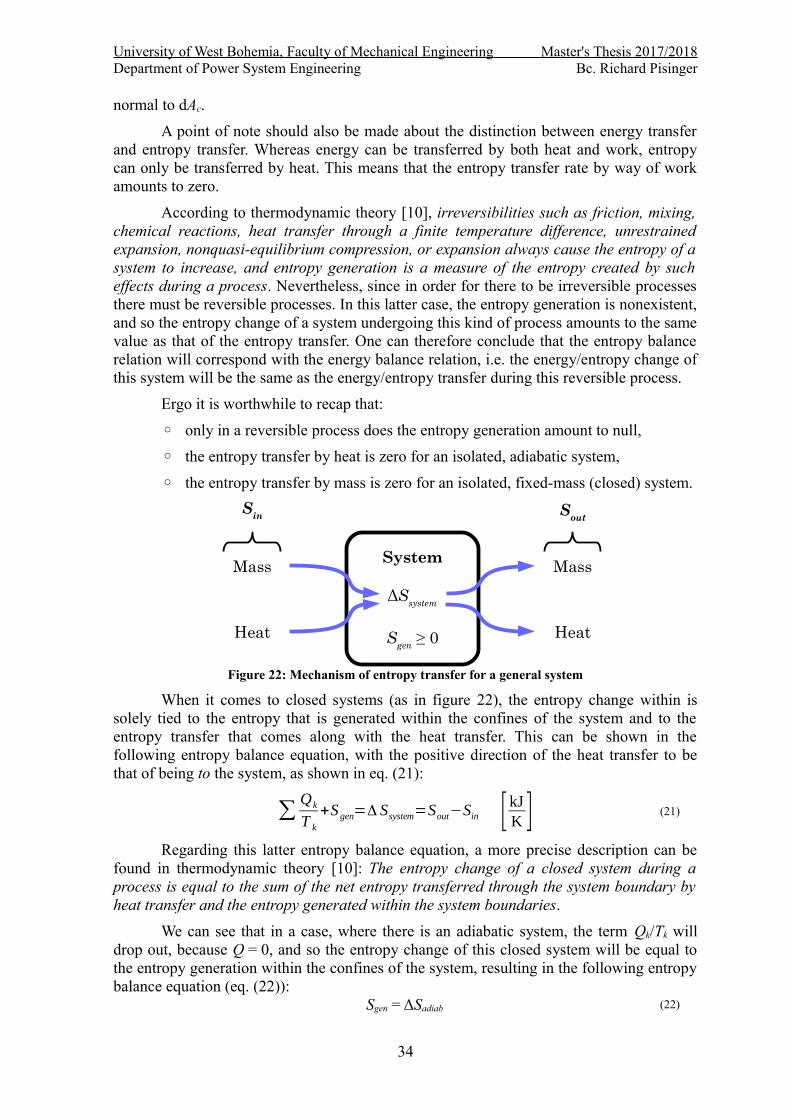
Figure 22: Mechanism of entropy transfer for a general system

When it comes to closed systems (as in figure 22), the entropy change within issolely tied to the entropy that is generated within the confines of the system and to theentropy transfer that comes along with the heat transfer. This can be shown in thefollowing entropy balance equation, with the positive direction of the heat transfer to bethat of being to the system, as shown in eq. (21):

∑Qk

T k

+S gen=Δ Ssystem=Sout−Sin [ kJK ] (21)

Regarding this latter entropy balance equation, a more precise description can befound in thermodynamic theory [10]: The entropy change of a closed system during aprocess is equal to the sum of the net entropy transferred through the system boundary byheat transfer and the entropy generated within the system boundaries.

We can see that in a case, where there is an adiabatic system, the term Qk/Tk willdrop out, because Q = 0, and so the entropy change of this closed system will be equal tothe entropy generation within the confines of the system, resulting in the following entropybalance equation (eq. (22)):

Sgen = ΔSadiab (22)

34

System

ΔSsystem

Sgen ≥ 0

Mass

Heat

Mass

Heat

Sin Sout


There is another aspect worthy of consideration, i.e. control volumes, as shown infigure 23. These differ from closed systems in that here there is mass flow across theboundaries of the system, which is another mechanism of entropy exchange. The entropybalance equation (eq. (22)) can be rewritten as equation (23), with the positive direction ofheat transfer being to the system:

(Sout−S in)CV=∑Qk

T k

+∑min⋅s in−∑mout⋅sout+Sgen (23)

Again, a reference is made to thermodynamic theory [10], for a more sophisticateddescription of this entropy balance relation: The rate of entropy change within the controlvolume during a process is equal to the sum of the rate of entropy transfer through thecontrol volume boundary by heat transfer, the net rate of entropy transfer into the controlvolume by mass flow, and the rate of entropy generation within the boundaries of thecontrol volume as a result of irreversibilities.

In the real world, most control volumes operate steadily, which means that there isno change in the entropy of these control volumes. An example of such a control volume isthe heat exchanger, which is part of the main topic of this thesis. The entropy balancerelation (eq. (23)) can be rewritten for a steady-flow process, by first applying dSCV/dt = 0,resulting in equation (24):

S gen=∑ mout⋅sout−∑ min⋅sin−∑Qk

T k

(24)

Figure 23: Entropy, heat, and mass transfer for a control volume (CV)

Equation (24) can be further simplified for a single-stream steady-flow apparatus,where there is only one inlet and one exit, resulting in equation (25):

S gen=m⋅(sout−sin)−∑Qk

T k

(25)

Equation (25) can be further simplified for use in an adiabatic single-stream device(eq. (26)):

S gen=m⋅(sout−sin) (26)

and since S gen≥0 , this implies that sout ≥ sin, which means that the specific entropy of the

35

Control Volume

me

se

mi

siT

Q

Surroundings

Δ SCV=QT⏟

Entropytransferby heat

+mi⋅si−me⋅se⏟Entropytransferby mass

+Sgen


fluid will never decrease as it flows through an adiabatic apparatus. If the flow turns out tobe both adiabatic and reversible, then sout = sin.

2.3 Entropy Generation MinimizationAccording to Bejan [11], “Entropy-generation minimization (EGM) is the method

of modeling and optimization of real devices that owe their thermodynamic imperfection toheat transfer, mass transfer, and fluid flow and other transport processes.” Bejan alsostates that, in the realm of engineering, this method can also be called thermodynamicoptimization. Another term for this can be found under finite time thermodynamics. He alsomakes mention of the usage of this method, that the EGM method involves itself in theareas of fluid mechanics, heat transfer, and thermodynamics.

The goals of optimization may differ significantly depending on the application it'sintended for. These can include, among other objectives, the minimization of power inputin a refrigeration plant, the maximization of power output in power plants, and in our casethe minimization of entropy generation in heat exchangers. These models all tend toinclude models which utilize rate processes, i.e. fluid flow, mass transfer, and/or heattransfer, fixed volumes of real apparatuses, and fixed speeds or times of actual processes.In order to optimize, one needs to include physical constraints onto the subject of theoptimization process; the irreversible operation of said device is dependent on theseconstraints. The fact is that the heat transfer model, combined with the thermodynamicsmodel, can provide a comprehensive visualization for the end analysis of the irreversiblenature of the apparatus. This further can show where and how much entropy is beinggenerated in the device, as well as where and how it flows, and how the thermodynamicperformance is affected as a result. [11]

The critical feature that characterizes the EGM method is the minimization of thecalculated entropy generation rate. This happens to also differentiate it from exergyanalysis. This method first requires the establishment of a way to express Sgen, i.e. entropygeneration. To go forward with this process, relations between the heat transfer rates andtemperature differences and between mass flow rates and pressure differences need to beset up. There is also a need to define the scope of the thermodynamic nonideality of thesystem to the physical characteristics thereof; e.g. the dimensions, the configuration, thematerials, the shapes, the fixed speeds, and the fixed time intervals of operation. This willinvariably involve referencing principles from the realm of fluid mechanics and heattransfer, notwithstanding thermodynamics. In order to actually bring a system, which issubjected to fixed time and fixed size constraints, closer to a situation characterized byminimum entropy generation, one would need to change only one or more of the physicalproperties of the system.

36


3 Developing the mathematical modelThe generation of entropy is significantly intertwined with the two laws of

thermodynamics. According to the first law, energy cannot be created or destroyed; it canonly be transformed from one form of energy to another form. The second law deals morespecifically with entropy in that “in all energy exchanges, if no energy enters or leaves thesystem, the potential energy of the state will always be less than that of the initial state.”This indirectly refers to the fact that losses are inevitable in real cycles, due toirreversibilities and effectiveness. This means that the entropy will increase. Therefore, themathematical model dealing with the generation of entropy will derive from the secondlaw. [12]

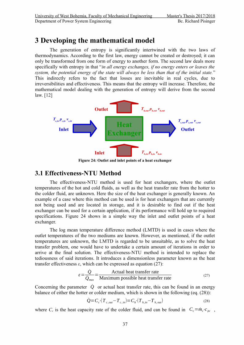
Figure 24: Outlet and inlet points of a heat exchanger

3.1 Effectiveness-NTU MethodThe effectiveness-NTU method is used for heat exchangers, where the outlet

temperatures of the hot and cold fluids, as well as the heat transfer rate from the hotter tothe colder fluid, are unknown. Here the size of the heat exchanger is generally known. Anexample of a case where this method can be used is for heat exchangers that are currentlynot being used and are located in storage, and it is desirable to find out if the heatexchanger can be used for a certain application, if its performance will hold up to requiredspecifications. Figure 24 shows in a simple way the inlet and outlet points of a heatexchanger.

The log mean temperature difference method (LMTD) is used in cases where theoutlet temperatures of the two mediums are known. However, as mentioned, if the outlettemperatures are unknown, the LMTD is regarded to be unsuitable, as to solve the heattransfer problem, one would have to undertake a certain amount of iterations in order toarrive at the final solution. The effectiveness-NTU method is intended to replace thetediousness of said iterations. It introduces a dimensionless parameter known as the heattransfer effectiveness ε, which can be expressed as equation (27):

ε=QQmax

=Actual heat transfer rate

Maximum possible heat transfer rate(27)

Concerning the parameter Q or actual heat transfer rate, this can be found in an energybalance of either the hotter or colder medium, which is shown in the following (eq. (28)):

Q=Cc⋅(T c ,out−T c , in)=Ch⋅(T h,in−T h, out) (28)

where Cc is the heat capacity rate of the colder fluid, and can be found in Cc=mc⋅c pc ,

37

HeatExchanger

Th,in

ph,in

vh,in

Th,out

ph,out

vh,out

Tc,in

pc,in

vc,in T

c,out p

c,out v

c,out

Outlet

Outlet

Inlet

Inlet


where mc is the mass transfer rate of the cold fluid, and cpc is the heat capacity of the coldfluid at a constant pressure. Replacing the index c with h, one obtains the same quantitiesfor the hot fluid.

In the ε-NTU method, one needs to first identify the maximum temperaturedifference of a heat exchanger, i.e. the temperature difference between the inlettemperatures of the cold and hot mediums, the formula of which can be found in thefollowing (eq. (29)):

ΔT max=T h ,in−T c ,in (29)

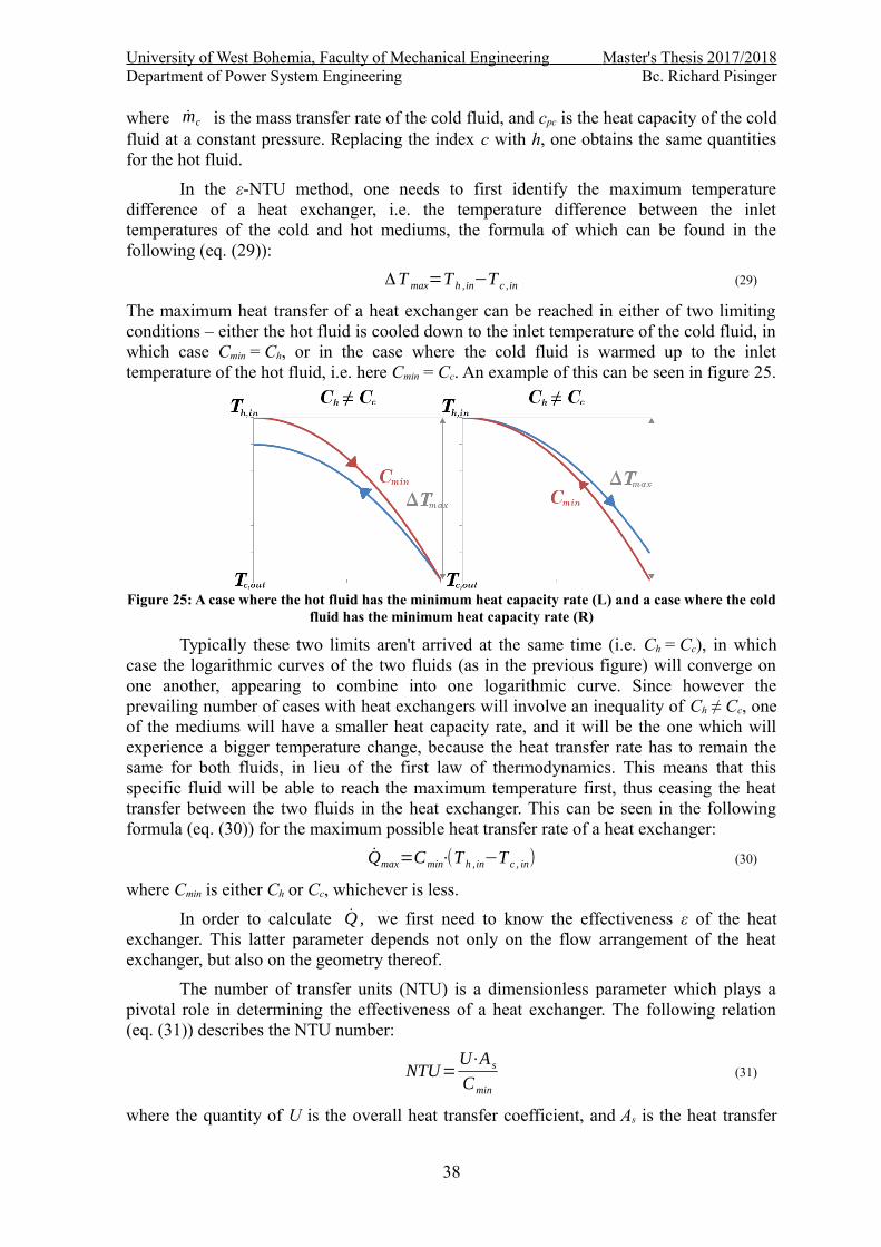
The maximum heat transfer of a heat exchanger can be reached in either of two limitingconditions – either the hot fluid is cooled down to the inlet temperature of the cold fluid, inwhich case Cmin = Ch, or in the case where the cold fluid is warmed up to the inlettemperature of the hot fluid, i.e. here Cmin = Cc. An example of this can be seen in figure 25.

Figure 25: A case where the hot fluid has the minimum heat capacity rate (L) and a case where the coldfluid has the minimum heat capacity rate (R)

Typically these two limits aren't arrived at the same time (i.e. Ch = Cc), in whichcase the logarithmic curves of the two fluids (as in the previous figure) will converge onone another, appearing to combine into one logarithmic curve. Since however theprevailing number of cases with heat exchangers will involve an inequality of Ch ≠ Cc, oneof the mediums will have a smaller heat capacity rate, and it will be the one which willexperience a bigger temperature change, because the heat transfer rate has to remain thesame for both fluids, in lieu of the first law of thermodynamics. This means that thisspecific fluid will be able to reach the maximum temperature first, thus ceasing the heattransfer between the two fluids in the heat exchanger. This can be seen in the followingformula (eq. (30)) for the maximum possible heat transfer rate of a heat exchanger:

Qmax=Cmin⋅(T h ,in−T c , in) (30)

where Cmin is either Ch or Cc, whichever is less.

In order to calculate Q , we first need to know the effectiveness ε of the heatexchanger. This latter parameter depends not only on the flow arrangement of the heatexchanger, but also on the geometry thereof.

The number of transfer units (NTU) is a dimensionless parameter which plays apivotal role in determining the effectiveness of a heat exchanger. The following relation(eq. (31)) describes the NTU number:

NTU=U⋅A s

Cmin

(31)

where the quantity of U is the overall heat transfer coefficient, and As is the heat transfer

38


surface area of the heat exchanger. It can be pointed out that the value of As plays a directrole in the size of the value of NTU, i.e. the larger the value of NTU, the larger the size ofthe heat exchanger.

It can often be found in literature regarding heat exchangers that there is anadditional defined dimensionless quantity known as the capacity ratio c, which is shownhere in equation (32):

c=Cmin

Cmax

(32)

Thus the effectiveness of a heat exchanger is directly a function of the NTUnumber and the capacity ratio c (eq. (33)):

ε=f (NTU ,c) (33)

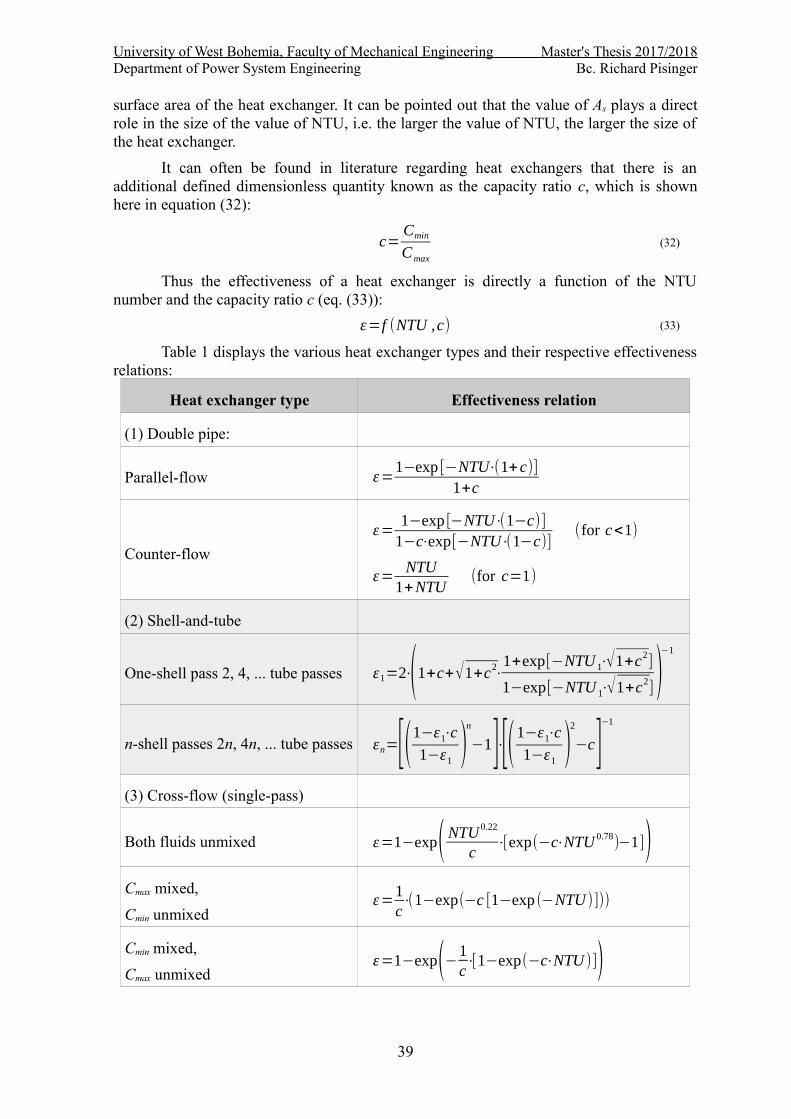
Table 1 displays the various heat exchanger types and their respective effectivenessrelations:

Heat exchanger type Effectiveness relation

(1) Double pipe:

Parallel-flow ε=1−exp [−NTU⋅(1+c)]

1+c

Counter-flow

ε=1−exp [−NTU⋅(1−c)]

1−c⋅exp[−NTU⋅(1−c)](for c<1)

ε= NTU1+NTU

(for c=1)

(2) Shell-and-tube

One-shell pass 2, 4, ... tube passes ε1=2⋅(1+c+√1+c2⋅

1+exp[−NTU 1⋅√1+c2]

1−exp[−NTU 1⋅√1+c2])

−1

n-shell passes 2n, 4n, ... tube passes εn=[(1−ε1⋅c

1−ε1)n

−1]⋅[(1−ε1⋅c

1−ε1)

2

−c]−1

(3) Cross-flow (single-pass)

Both fluids unmixed ε=1−exp(NTU0.22

c⋅[exp(−c⋅NTU 0.78)−1])

Cmax mixed,

Cmin unmixedε=1

c⋅(1−exp(−c [1−exp (−NTU )]))

Cmin mixed,

Cmax unmixedε=1−exp(−1

c⋅[1−exp(−c⋅NTU )])

39


Heat exchanger type Effectiveness relation

(4) All heat exchangers with c = 0 ε=1−exp(−NTU )

Table 1: Effectiveness relations for heat exchangers [13]

(a) Parallel-flow (b) Counter-flow

(c) One-shell pass and 2,4,6, … tube passes (d) Two-shell passes and 4, 8, 12, … tube passes

40


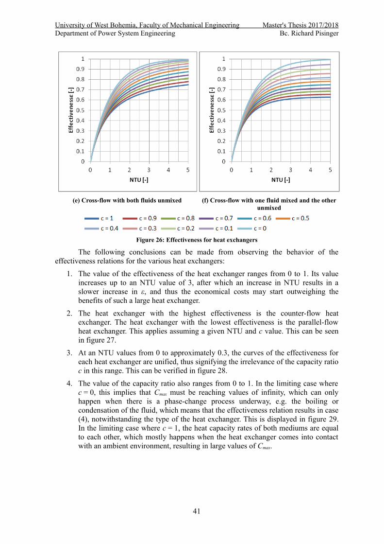
(e) Cross-flow with both fluids unmixed (f) Cross-flow with one fluid mixed and the otherunmixed

Figure 26: Effectiveness for heat exchangers

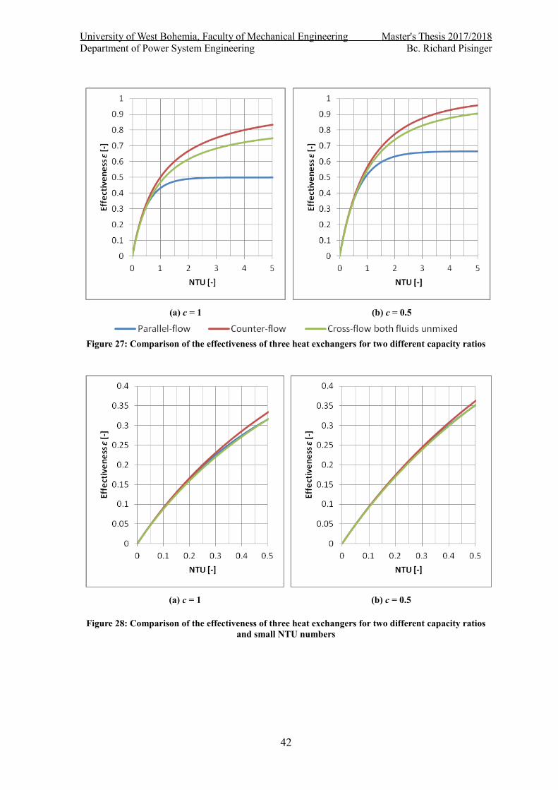
The following conclusions can be made from observing the behavior of theeffectiveness relations for the various heat exchangers:

1. The value of the effectiveness of the heat exchanger ranges from 0 to 1. Its valueincreases up to an NTU value of 3, after which an increase in NTU results in aslower increase in ε, and thus the economical costs may start outweighing thebenefits of such a large heat exchanger.

2. The heat exchanger with the highest effectiveness is the counter-flow heatexchanger. The heat exchanger with the lowest effectiveness is the parallel-flowheat exchanger. This applies assuming a given NTU and c value. This can be seenin figure 27.

3. At an NTU values from 0 to approximately 0.3, the curves of the effectiveness foreach heat exchanger are unified, thus signifying the irrelevance of the capacity ratioc in this range. This can be verified in figure 28.

4. The value of the capacity ratio also ranges from 0 to 1. In the limiting case wherec = 0, this implies that Cmax must be reaching values of infinity, which can onlyhappen when there is a phase-change process underway, e.g. the boiling orcondensation of the fluid, which means that the effectiveness relation results in case(4), notwithstanding the type of the heat exchanger. This is displayed in figure 29.In the limiting case where c = 1, the heat capacity rates of both mediums are equalto each other, which mostly happens when the heat exchanger comes into contactwith an ambient environment, resulting in large values of Cmax.

41


(a) c = 1 (b) c = 0.5

Figure 27: Comparison of the effectiveness of three heat exchangers for two different capacity ratios

(a) c = 1 (b) c = 0.5

Figure 28: Comparison of the effectiveness of three heat exchangers for two different capacity ratiosand small NTU numbers

42


Figure 29: Effectiveness as a relation of NTU for c = 0 for all heat exchangers

The NTU value, or the size of the heat exchanger, can also be determined in reversewhen the outlet temperatures are known from the basic definition of ε and then fromtable 2.

Heat exchanger type NTU relation

(1) Double-pipe

Parallel-flow NTU=−ln [1−ε (1+c)]

1+c

Counter-flow

NTU=1

c−1⋅ln( ε−1

ε⋅c−1 ) (for c<1)

NTU=ε

1−ε(for c=1)

(2) Shell and tube:

One-shell pass 2, 4, ... tube passes NTU 1=−1

√1+c2⋅ln(2 / ε1−1−c−√1+c2

2 /ε1−1−c+√1+c2 )

n-shell passes 2n, 4n, ... tube passes

NTU n=n⋅(NTU )1

To find the effectiveness of a heat exchanger with one-shell

pass use, ε1=F−1F−c

where F=( εn⋅c−1

εn−1 )1 /n

43


Heat exchanger type NTU relation

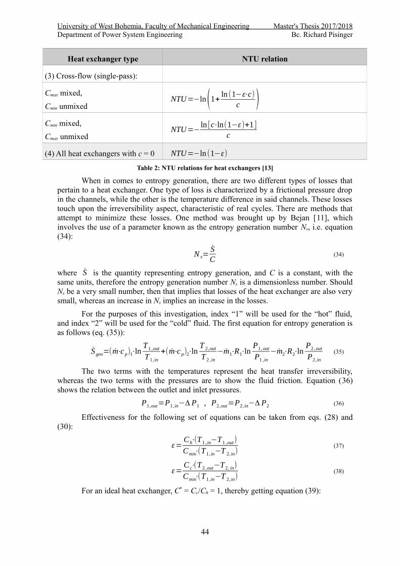
(3) Cross-flow (single-pass):

Cmax mixed,

Cmin unmixedNTU=−ln(1+

ln (1−ε⋅c)c )

Cmin mixed,

Cmax unmixedNTU=−

ln [c⋅ln(1−ε )+1 ]

c

(4) All heat exchangers with c = 0 NTU=−ln (1−ε)

Table 2: NTU relations for heat exchangers [13]

When in comes to entropy generation, there are two different types of losses thatpertain to a heat exchanger. One type of loss is characterized by a frictional pressure dropin the channels, while the other is the temperature difference in said channels. These lossestouch upon the irreversibility aspect, characteristic of real cycles. There are methods thatattempt to minimize these losses. One method was brought up by Bejan [11], whichinvolves the use of a parameter known as the entropy generation number Ns, i.e. equation(34):

N s=SC

(34)

where S is the quantity representing entropy generation, and C is a constant, with thesame units, therefore the entropy generation number Ns is a dimensionless number. ShouldNs be a very small number, then that implies that losses of the heat exchanger are also verysmall, whereas an increase in Ns implies an increase in the losses.

For the purposes of this investigation, index “1” will be used for the “hot” fluid,and index “2” will be used for the “cold” fluid. The first equation for entropy generation isas follows (eq. (35)):

S gen=(m⋅c p)1⋅lnT 1 ,out

T 1 , in

+(m⋅c p)2⋅lnT 2,out

T 2 , in

−m1⋅R1⋅lnP1 , out

P1 , in

−m2⋅R2⋅lnP2 ,out

P2 , in

(35)

The two terms with the temperatures represent the heat transfer irreversibility,whereas the two terms with the pressures are to show the fluid friction. Equation (36)shows the relation between the outlet and inlet pressures.

P1 ,out=P1 , in−Δ P1 , P2 ,out=P2 , in−Δ P2 (36)

Effectiveness for the following set of equations can be taken from eqs. (28) and(30):

ε=Ch⋅(T 1 , in−T 1 ,out)

Cmin⋅(T 1 , in−T 2 , in)(37)

ε=C c⋅(T 2 ,out−T 2 , in)

Cmin⋅(T 1 , in−T 2 , in)(38)

For an ideal heat exchanger, C* = Cc/Ch = 1, thereby getting equation (39):

44


ε=(T 1 , in−T 1 ,out)

(T 1 , in−T 2 , in)=

(T 2 ,out−T 2 , in)

(T 1 , in−T 2 , in)(39)

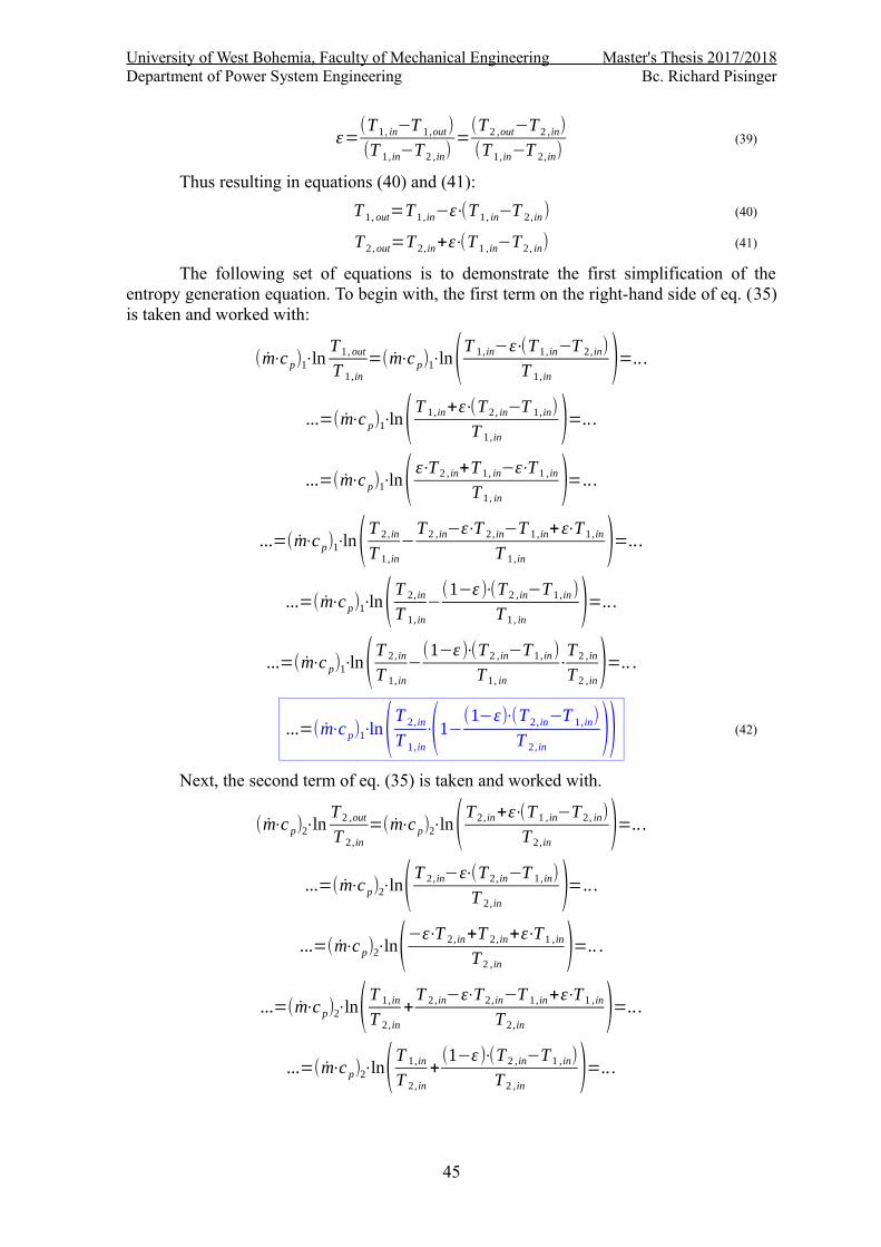
Thus resulting in equations (40) and (41):

T 1 , out=T 1 , in−ε⋅(T 1 , in−T 2 , in) (40)

T 2 , out=T 2 , in+ε⋅(T 1 , in−T 2 , in) (41)

The following set of equations is to demonstrate the first simplification of theentropy generation equation. To begin with, the first term on the right-hand side of eq. (35)is taken and worked with:

(m⋅c p)1⋅lnT 1 , out

T 1 , in

=(m⋅c p)1⋅ln(T 1 , in−ε⋅(T 1 , in−T 2 , in)

T 1 , in)=.. .

...=(m⋅c p)1⋅ln(T 1 , in+ε⋅(T 2 , in−T 1 , in)

T 1 , in)=.. .

...=(m⋅c p)1⋅ln( ε⋅T 2 , in+T 1 , in−ε⋅T 1 , in

T 1 , in)=.. .

...=(m⋅c p)1⋅ln(T 2 , in

T 1 , in

−T 2 , in−ε⋅T 2 , in−T 1 , in+ε⋅T 1 , in

T 1 , in)=.. .

...=(m⋅c p)1⋅ln(T 2, in

T 1, in

−(1−ε )⋅(T 2 , in−T 1 , in)

T 1 , in)=.. .

...=(m⋅c p)1⋅ln(T 2, in

T 1, in

−(1−ε )⋅(T 2 , in−T 1 , in)

T 1 , in

⋅T 2 , in

T 2 , in)=.. .

...=(m⋅c p)1⋅ln(T 2 , in

T 1 , in

⋅(1−(1−ε)⋅(T 2 , in−T 1 , in)

T 2 , in)) (42)

Next, the second term of eq. (35) is taken and worked with.

(m⋅c p)2⋅lnT 2 ,out

T 2 , in

=(m⋅c p)2⋅ln(T 2 , in+ε⋅(T 1 , in−T 2 , in)

T 2 , in)=.. .

...=(m⋅c p)2⋅ln(T 2 , in−ε⋅(T 2 , in−T 1 , in)

T 2 , in)=.. .

...=(m⋅c p)2⋅ln(−ε⋅T 2 , in+T 2 , in+ε⋅T 1 , in

T 2 , in)=.. .

...=(m⋅c p)2⋅ln(T 1, in

T 2, in

+T 2 , in−ε⋅T 2 , in−T 1 , in+ε⋅T 1 , in

T 2 , in)=.. .

...=(m⋅c p)2⋅ln(T 1 , in

T 2 , in

+(1−ε)⋅(T 2 , in−T 1 , in)

T 2 , in)=.. .

45


...=(m⋅c p)2⋅ln(T 1 , in

T 2 , in

+(1−ε )⋅(T 2 , in−T 1 , in)

T 2 , in

⋅T 1 , in

T 1 , in)=.. .

...=(m⋅c p)2⋅ln(T 1 , in

T 2 , in

⋅(1+(1−ε )⋅(T 2 , in−T 1 , in)

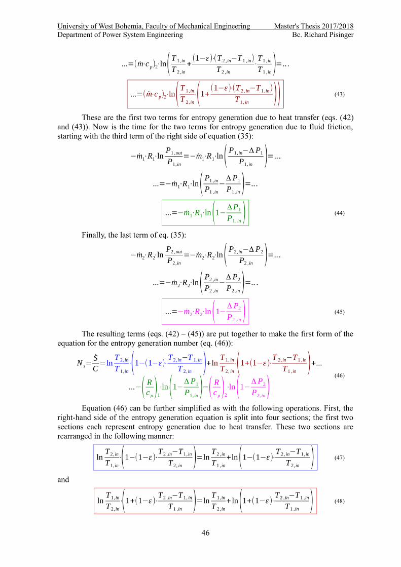
T 1 , in)) (43)

These are the first two terms for entropy generation due to heat transfer (eqs. (42)and (43)). Now is the time for the two terms for entropy generation due to fluid friction,starting with the third term of the right side of equation (35):


P1 , in

=−m1⋅R1⋅ln(P1 , in−Δ P1

P1 , in)=.. .

...=−m1⋅R1⋅ln(P1 , in

P1 , in

−Δ P1

P1 , in)=.. .

...=−m1⋅R1⋅ln(1−ΔP1

P1 , in) (44)

Finally, the last term of eq. (35):


P2 , in

=−m2⋅R2⋅ln(P2 , in−Δ P2

P2 , in)=.. .

...=−m2⋅R2⋅ln(P2 ,in

P2 ,in

−Δ P2

P2 , in)=.. .

...=−m2⋅R2⋅ln(1−Δ P2

P2 , in) (45)

The resulting terms (eqs. (42) – (45)) are put together to make the first form of theequation for the entropy generation number (eq. (46)):

N s=SC

=lnT 2 , in

T 1 , in

⋅(1−(1−ε)⋅T 2 , in−T 1 , in

T 2 , in)+ln

T 1 , in

T 2 , in

⋅(1+(1−ε )⋅T 2 , in−T 1 , in

T 1 , in)+...

...−( Rc p)1

⋅ln(1−Δ P1

P1 , in)−( Rc p

)2

⋅ln(1−Δ P2

P2 , in)

(46)

Equation (46) can be further simplified as with the following operations. First, theright-hand side of the entropy generation equation is split into four sections; the first twosections each represent entropy generation due to heat transfer. These two sections arerearranged in the following manner:

lnT 2 , in

T 1 , in

⋅(1−(1−ε )⋅T2 ,in−T 1 , in

T 2 , in)=ln

T 2 , in

T 1 , in

+ln(1−(1−ε )⋅T 2 , in−T 1 , in

T 2 , in) (47)

and

lnT 1 , in

T 2 , in

⋅(1+(1−ε )⋅T 2 , in−T 1 , in

T 1 ,in)=ln

T 1 , in

T 2 , in

+ ln(1+(1−ε )⋅T 2 , in−T 1 , in

T 1 , in) (48)

46


Here the following equation applies:

lnT 2 , in

T 1 , in

+lnT 1 , in

T 2 , in

=lnT 2 , in

T 1 , in

⋅T 1 , in

T 2 , in

=0 (49)

Applying eq. (49) on eq. (47), we get eq. (50):

ln(1−(1−ε)⋅T 2 , in−T 1 , in

T 2 , in) (50)

and similarly, applying eq. (49) on eq. (48), we get eq. (51):

ln(1+(1−ε )⋅T 2 , in−T 1 , in

T 1 , in) (51)

The relation for heat exchanger effectiveness is significantly smaller than unity:

(1−ε )≪1 (52)

Resulting in the first two sections being as follows, i.e. applying eq. (52) on eq.(50) to get eq. (53) and similarly applying eq. (52) on eq. (51) to get eq. (54):

ln(1−(1−ε)⋅T 2 , in−T 1 , in

T 2 , in)≃−(1−ε )⋅

T 2 , in−T 1 , in

T 2 , in

(53)

ln(1+(1−ε )⋅T 2 , in−T 1 , in

T 1 , in)≃(1−ε )⋅

T 2 , in−T 1 , in

T 1 , in

(54)

The first two sections (eqs. (53) and (54)) are put together, in order to end up withequation (55):

−(1−ε )⋅T 2 , in−T 1 ,in

T 2 , in

+(1−ε )⋅T 2 , in−T 1 , in

T 1 , in

=.. .

...=(1−ε )⋅(T 2 , in−T 1 , in)⋅(− 1T 2 , in

+1

T 1 , in)=.. .

...=(1−ε )⋅(T 2 , in−T 1 , in)⋅(− T 1 , in

T 2 , in⋅T 1, in

+T 2 , in

T 1 , in⋅T 2 , in)=.. .

...=(1−ε )⋅(T 2 , in−T 1 , in)⋅(T 2 , in−T 1 , in

T 2 , in⋅T 1 , in)=.. .

...=(1−ε )⋅(T 2 , in−T 1 , in)

2

T 2 , in⋅T 1 , in

(55)

Now that one side of the right-hand side of the simplified equation for the entropygeneration number (eq. (46)) has been achieved, the part of eq. (46) with the pressure terms

47


will be further simplified, as per the following procedures:

−Rc p

⋅ln(1−ΔP1

P1 , in)− R

c p

⋅ln(1−Δ P2

P2 , in)=−

Rc p

⋅(ln(1−Δ P1

P1 , in)+ln(1−

Δ P2

P2 , in)) (56)

where for an ideal heat exchanger,Rc p

=( Rc p)1

=( Rc p )2.

The pressure term is considerably smaller than unity (eq. (57)):

(Δ PPin )1,2

≪1 (57)

Which results in the following operations (eq. (58)):

⇒−Rc p

⋅(−Δ P1

P1 , in

−Δ P2

P2 , in)=.. .

...=Rc p

⋅(Δ P1

P1 , in

+Δ P2

P2 , in) (58)

Now that we have the pressure terms of equation (46), the entire simplifiedequation for the entropy generation number is as follows (eq. (59)):

N s=(1−ε )⋅(T 2 , in−T 1 , in)

2

T 2 ,in⋅T 1 , in

+Rc p

⋅(Δ P1

P1 , in

+Δ P2

P2 , in) (59)

In order to apply equation (59) for all of the heat exchangers, the effectiveness ε issubstituted with the equations from table 1, so as to get eqs. (60) – (63), listed in table 3.

Heat ExchangerType

Entropy Generation Equation

Double pipe:

Parallel-flow

N s=(1−1−exp [−NTU⋅(1+c )]

1+c )⋅(T 2 , in−T 1 , in)2

T 2 , in⋅T 1 , in

+...

...+Rcp

⋅(Δ P1

P1 , in

+Δ P2

P2 , in)

(60)

Counter-flow

c < 1

N s=(1−1−exp[−NTU⋅(1−c)]

1−c⋅exp [−NTU⋅(1−c )])⋅(T 2 , in−T 1 , in)

2

T 2 , in⋅T 1 , in

+...

...+ Rc p

⋅(Δ P1

P1 , in

+Δ P2

P2 , in)

(61)

48


Heat ExchangerType


c = 1

N s=(1− NTU1+NTU )⋅(T 2 , in−T 1 , in)

2

T 2 , in⋅T 1 , in

+...

...+Rc p

⋅(Δ P1

P1 , in

+Δ P2

P2 , in)

(62)

Cross-flow(single-pass)

Both fluidsunmixed

N s=(exp(NTU0.22

c⋅[exp(−c⋅NTU 0.78

)−1]))⋅......⋅

(T 2 , in−T 1 , in)2

T 2 , in⋅T 1 , in

+Rcp

⋅(Δ P1

P1 , in

+Δ P2

P2 , in)

(63)

Table 3: Modified entropy generation equations

It should be noted that one of the intended goals of the minimization of the entropygeneration number is to curtail losses in heat transfer. This means that it would be best torewrite the entropy generation equations using eqs. (64) – (68) for any heat exchangerdesign.

ΔT *=

|T 2 ,in−T 1 , in|

√T 1 ,in⋅T 2 , in

(64)

(Δ P1

P1 , in

+Δ P2

P2 , in)=(Δ P

Pin )1,2

=f⋅4⋅LD

⋅G2

2⋅ρ⋅P(65)

NTU=4⋅LD

⋅St (66)

G*=

G

√2⋅ρ⋅P(67)

St=Nu

Re⋅Pr(68)

The equations for entropy generation ((69) – (72)) can now be rewritten as listed intable 4.

49


Heat ExchangerType


Double pipe:

Parallel-flowN s=(1−

1−exp[−4⋅LD

⋅St⋅(1+c )]1+c )⋅(ΔT *

)2+...

...+ Rc p

⋅f⋅(4⋅LD )⋅(G*

)2

(69)

Counter-flow

c < 1

N s=(1−1−exp[− 4⋅L

D⋅St⋅(1−c)]

1−c⋅exp[−4⋅LD

⋅St⋅(1−c )])⋅(ΔT *)

2+...

...+Rc p

⋅f⋅( 4⋅LD )⋅(G*

)2

(70)

c = 1 N s=(1−

4⋅LD

⋅St

1+4⋅LD

⋅St )⋅(ΔT *)

2+Rc p

⋅f⋅(4⋅LD )⋅(G*

)2

(71)


Both fluidsunmixed

N s=(exp[(4⋅LD

⋅St)0.22

c⋅[exp(−c⋅( 4⋅L

D⋅St)

0.78

)−1]])⋅......⋅(ΔT *

)2+Rc p

⋅f⋅(4⋅LD )⋅(G*

)2

(72)

Table 4: Modified entropy generation equations

50


3.2 Sensitivity analysis of the mathematical modelIn order to figure out which parameter of the mathematical model is going to have

the greatest influence and effect on the entropy generation number, a sensitivity analysisneeds to be done. This is done by first differentiating the equation for the entropygeneration number into first order, second order, and third order derivatives. It is alsoimportant to have a NOP (Normal Operating Point), which serves as a reference point, i.e.the initial values of the parameters of the model. Thereupon a relative sensitivity analysis isperformed, to see which parameter has the greatest influence on the generation of entropy.

An example of how to derive the equation is shown in the following set ofequations, by first taking a modified version of eq. (35):

Cmin⋅(ln(T 1 ,out

T 1 , in)+( Rc p)1

⋅ln( P1 , in

P1 ,out))+Cmax⋅(ln( P2 , in

P2 ,out)⋅( Rc p)2

+ ln(T 2 , out

T 2 , in)) (73)

For this example, equation (73) is differentiated by the parameter of T1,out:

∂ S∂T 1 , out

=Cmin⋅( ∂∂T 1 ,out (ln(T 1 ,out

T 1 , in))+ ∂

∂T 1 ,out (( Rc p)1

⋅ln( P1 , in

P1 , out)))+...

...+ ∂∂T 1 ,out (Cmax⋅(ln( P2 , in

P2 ,out)⋅( Rc p)2

+ ln(T 2 , out

T 2 , in)))=.. .

...=( T 1 , in

T 1 ,out

⋅ ∂∂T 1 ,out

(T 1 ,out

T 1 , in)+0)⋅Cmin+0=

1T 1 , in

⋅ ∂∂T 1 ,out

(T 1 ,out)⋅T 1 , in⋅Cmin

T 1 ,out

=.. .

...= ∂ S∂T 1 ,out

=Cmin

T 1 ,out

∂ S∂T 1 , out

=(m⋅c p)1

T 1 , out

(74)

The derivatives (eqs. (75) – (110)) have been arranged into table 5 for clarity:

Order Derivative

1∂ S

∂T 1 , out

=(m⋅c p)1

T 1 , out

(75)

1∂ S

∂T 1 , in

=−(m⋅cp)1

T 1 , in

(76)

1∂ S

∂T 2 , out

=(m⋅c p)2

T 2 , out

(77)

51


Order Derivative

1∂ S

∂T 2 , in

=−(m⋅c p)2

T 2 , in

(78)

1∂ S

∂P1 ,out

=−m1⋅R1

P1 ,out

(79)

1∂ S

∂P1 , in

=m1⋅R1

P1 , in

(80)

1∂ S

∂P2 ,out

=−m2⋅R2

P2 ,out

(81)

1∂ S

∂P2 , in

=m2⋅R2

P2 , in

(82)

1∂ S

∂Cmin

=( Rc p )1

⋅ln( P1 , in

P1 ,out)+ln(T 1 , out

T 1 , in) (83)

1∂ S

∂Cmax

=( Rcp )2

⋅ln( P2 , in

P2 ,out)+ln(T 2 ,out

T 2 , in) (84)

1∂ S

∂( Rc p)1

=(m⋅c p)1⋅ln( P1 , in

P1 , out) (85)

1∂ S

∂( Rc p)2

=(m⋅cp)2⋅ln( P2 , in

P2 , out) (86)

2∂

2 S

∂T 1 , out2

=−(m⋅c p)1

T 1 ,out2 (87)

2∂

2 S∂T 1 , out∂Cmin

=1

T 1 ,out

(88)

2∂

2 S

∂T 1 , in2

=(m⋅c p)1

T 1 , in2 (89)

2∂

2 S∂T 1 , in∂Cmin

=−1

T 1 , in

(90)

2∂

2 S

∂T 2 , out2

=−(m⋅c p)2

T 2 ,out2 (91)

52


Order Derivative

2∂

2 S∂T 2 , out∂Cmax

=1

T 2 ,out

(92)

2∂

2 S

∂T 2 , in2

=(m⋅c p)2

T 2 , in2 (93)

2∂

2 S∂T 2 , in∂Cmax

=−1

T 2 , in

(94)

2∂

2 S

∂P1 ,out2

=m1⋅R1

P1 , out2 (95)

2∂

2 S∂P1 ,out ∂Cmin

=−1

P1 ,out

⋅( Rc p )1

(96)

2

∂2 S

∂P1 ,out ∂( Rc p )1

=−(m⋅c p)1

P1 , out (97)

2∂

2 S

∂P1 , in2

=−m1⋅R1

P1 , in2 (98)

2∂

2 S∂P1 , in∂Cmin

=1

P1 , in

⋅( Rc p)1

(99)

2

∂2 S

∂P1 , in∂( Rcp )1

=(m⋅c p)1

P1 , in (100)

2∂

2 S

∂P2 ,out2

=m2⋅R2

P2 ,out2 (101)

2∂

2 S∂P2 ,out ∂Cmax

=−1

P2 ,out

⋅( Rc p)2

(102)

2

∂2 S

∂P2 ,out ∂( Rc p )2

=−(m⋅c p)2

P2 ,out (103)

2∂

2 S

∂P2 , in2

=−m2⋅R2

P2 , in2 (104)

53


Order Derivative

2∂

2 S∂P2 , in∂Cmax

=1

P2 , in

⋅( Rc p )2

(105)

2

∂2 S

∂P2 , in∂( Rc p)2

=(m⋅c p)2

P2 , in (106)

3∂

3 S

∂P1 ,out ∂Cmin∂( Rc p )1

=−1

P1 , out (107)

3∂

3 S

∂P1 , in∂Cmin∂( Rc p )1

=1

P1 , in (108)

3∂

3 S

∂P2 ,out ∂Cmax∂( Rc p)2

=−1

P2 ,out (109)

3∂

3 S

∂P2 , in∂Cmax∂( Rc p)2

=1

P2 , in (110)

Table 5: Table of derivatives for the sensitivity analysis

It should be noted for the sake of clarity that partial derivatives are continuous, i.e.it doesn't matter in which order the partial differentiations are formed, e.g.

∂2 f

∂ x⋅∂ y=

∂2 f

∂ y⋅∂ x. Ergo, no additional second-order or third-order derivatives are

necessary.

The next part that is needed for the sensitivity analysis is to have the initial valuesfor the parameters, i.e. the Normal Operating Point (NOP). These are placed in table 6. Forthe purposes of analysis, the values were arbitrarily selected based on experimental valuesfound in literature [14], which deals with a similar topic.

Parameter Value Unit

T1out 430.15 K

T1in 450.15 K

P1out 800 kPa

P1in 500 kPa

54


Parameter Value Unit

T2out 440.15 K

T2in 415.15 K

P2out 300 kPa

P2in 200 kPa

R1 461.5 J/(kg∙K)

m1 0.4 kg/s

cp1 2500 J/(kg∙K)

Cmin 1000 J/(s∙K)

R2 461.5 J/(kg∙K)

m2 0.4 kg/s

cp2 4200 J/(kg∙K)

Cmax 1680 J/(s∙K)

Table 6: Normal Operating Point (NOP)

To figure out which parameter, when subjected to a change in value, will have thegreatest effect on the change in value of the entropy generation number, one simply insertsthe values of the NOP into any of the derivatives listed previously, and then multiplying theresult by the normal value of the parameter and at the same time dividing it by the normalvalue of the function (i.e. the value of the entropy generation function with all of the valuesof the NOP inserted). This is known as a relative-sensitivity analysis. The basic structure ofhow to work with the relative-sensitivity analysis can be seen in the following equation(111), taken from Smith et al. [15]:

SαF=

∂F∂α |NOP

⋅α 0

F0

≈% change in F% change in α

=

Δ FF

Δαα

(111)

An example of how this works is in the following set of equations (Eqs. (112) and(113)).

The value of the entropy generation function with all of the values of the NOPinserted:

S0=1000⋅(ln(430.15450.15)+(

461.52500 )⋅ln(800

500 ))+...

...+1680⋅(ln(440.15415.15)+(

461.54200 )⋅ln(200

300))=...

...=64.7060732 [-]

(112)

55


The value of the first listed derivative using the relative-sensitivity analysis:

ST1 ,out

S=

∂ S∂T 1, out|NOP

⋅T 1 ,out 0

S0

=(m⋅cp)1

T 1 ,out

⋅T 1, out

S0

=...

...=0.4⋅2500430.15

⋅430.15

64.7060732=15.4544999 [- ]

(113)

Figure 30 illustrates the relative sensitivity of each derivative in a simplifiedformat.

Figure 30: Relative-sensitivity analysis for the entropy generation function

It appears that the second-order and third-order derivatives seem to have the lowestinfluence on the value of the entropy generation function, therefore their visualization isrelegated to the top-right corner. The greatest influence on the change in the entropygeneration value is from the inlet and outlet temperatures of the second fluid, i.e. T2out andT2in. This appears to be what also occurred in the work of Koorts [14], where the greatestaverage change in entropy generation came from a 30K temperature change in the steaminlet temperature (103.6%) and in the steam outlet temperature (72.83%). In the case ofthis thesis, the change in entropy generation stemming from a change in temperature of thesecond fluid of either the outlet or inlet is the same (±25,96 [-]), the congruence of whichcan be observed in figure (30). This congruity can also be observed for T1in, T1out, P1in, P1out,P2in, and P2out.

56

15.45

-15.45

25.96

-25.96

-2.85

2.85

-2.85

2.850.64 0.36 1.34

-0.04

∂ S

∂( Rcp)2

∂ S

∂( Rcp)1

∂ S∂Cmax

∂ S∂Cmin

∂ S∂P2 ,in

∂ S∂P2 ,out

∂ S∂P1 ,in

∂ S∂P1 ,out

∂ S∂T2 , in

∂ S∂T2 , out

∂ S∂T1 , in

∂ S∂T1 , out

1st ord.

2nd order

3rd ord.


3.3 Graphs and resultsThe results of the mathematical model in this thesis can be seen in figures 31 – 40

as trends between the optimum flow path length ((4L/D)opt) and the dimensionless massvelocity (G*) for the three basic types of heat exchangers analyzed here, i.e. the parallel-flow heat exchanger, the counter-flow heat exchanger, and the cross-flow heat exchanger.For each of the heat exchangers, a variant with c = 0.595238095238095 was developed anda variant with c = 1 was developed. The value of c = 0.595238095238095 was chosenbecause it was used in the analysis by Ogulata et al. [16]. The results were first validatedwith the cross-flow heat exchanger, because it was the same type of heat exchanger thatwas used by the Ogulata et al. [16].

0.03 0.04 0.05 0.06 0.07 0.08 0.090

10

20

30

40

50

60

70

80

90

100

Parallel-flow

Counter-flow c<1

Cross-flow

Ogulata

Dimensionless Mass Velocity G* [-]

Opt

imum

Flo

w P

ath

Leng

th (4

L/D

)_op

t [-]

Figure 31: Variation between the optimum flow path length and the dimensionless mass velocity for allof the heat exchangers with c = 0.595238095238095

Figure 31 for c < 1 displays the trendlines of how the optimum flow path lengthdepends on the dimensionless mass velocity for all three of the examined heat exchangers.It is evident that the Cross-flow heat exchanger here closely follows that of theexperimental data from Ogulata et al. [16]. The values for the dimensionless mass velocityon the horizontal axis were chosen to correspond with that of the literature with theexperimental data. Here the parallel-flow heat exchanger appears to have the lowest valuesfor the optimum flow path, while the cross-flow heat exchanger has the widest range.

In figure 32, one can observe again that the cross-flow heat exchanger follows theexperimental data closely. What is interesting is due to the mathematical nature of theequations for entropy generation (eqs. (69) – (72)), the functions could not be plotted forthe whole range that is shown on the horizontal axis (which is again the same range as thatused in Ogulata et al. [16]). For a given NOP, the parallel-flow heat exchanger has a rangeof 7 to approximately 32 for the optimum flow path length, which is the shortest range, asshown in the graph. What is more important to see is that is appears here that the counter-flow heat exchanger appears to be the best.

57


0 10 20 30 40 50 60 70 80 90 1000.000

0.002

0.004

0.006

0.008

0.010

0.012

Parallel-flow

Counter-flow c<1

Cross-flow

Ogulata

Optimum Flow Path Length (4L/D)_opt [-]

Min

imum

Ent

ropy

Gen

erat

ion

Num

ber (

Ns,

min

) [-]

Figure 32: Variation between the minimum entropy generation number and the optimum flow pathlength for all of the heat exchangers with c = 0.595238095238095

0.03 0.04 0.05 0.06 0.07 0.08 0.090

10

20

30

40

50

60

70

80

90

100

Parallel-flow

Counter-flow c=1

Cross-flow


Opt

imum

Flo

w P

ath

Leng

th (4

L/D

)_op

t [-]

Figure 33: Variation between the optimum flow path length and the dimensionless mass velocity for allof the heat exchangers with c = 1

Figure 33 shows the dependence of the optimum flow path length on thedimensionless mass velocity for heat exchangers with c = 1. Here the plot is similar tofigure 31, except that the counter-flow heat exchanger appears to more closely follow thecross-flow heat exchanger, intersecting once at about point [0.053 , 36].

The similarities do not end with figure 34, which shows stark resemblance to figure32, except that here the cross-flow heat exchanger appears to give higher entropygeneration values.

58


0 10 20 30 40 50 60 70 80 90 1000.00

0.01

0.01

0.02

0.02

0.03

Parallel-flow

Counter-flow c=1

Cross-flow


Min

imum

Ent

ropy

Gen

erat

ion

Num

ber (

Ns,

min

) [-]

Figure 34: Variation between the minimum entropy generation number and the optimum flow pathlength for all of the heat exchangers with c = 1

0.03 0.04 0.05 0.06 0.07 0.08 0.090

2

4

6

8

10

12

14

c=0.59

c=1


Opt

imum

Flo

w P

ath

Leng

th (4

L/D

)_op

t [-]

Figure 35: Optimum flow path comparison of parallel-flow heat exchangers

In figures 35 and 36 we can see plots comparing the heat capacity ratios for theparallel-flow heat exchanger. A smaller heat capacity ratio (c < 1) gives larger values forthe optimum flow path, while at the same time providing smaller values for the entropygeneration number.

59


7 8 9 10 11 12 13 140.000

0.001

0.001

0.002

0.002

0.003

0.003

0.004

0.004

c=0.59

c=1


Min

imum

Ent

ropy

Gen

erat

ion

Num

ber (

Ns,

min

) [-]

Figure 36: Minimum entropy generation number comparison of parallel-flow heat exchangers

0.03 0.04 0.05 0.06 0.07 0.08 0.090

10

20

30

40

50

60

70

c=0.59

c=1


Opt

imum

Flo

w P

ath

Leng

th (4

L/D

)_op

t [-]

Figure 37: Optimum flow path comparison of counter-flow heat exchangers

In figure 37 we can see a different scenario, where the smaller heat capacity ratio(c < 1) gives smaller values for the optimum flow path length. Figure 38 shows a gapbetween the two functions for the counter-flow heat exchanger. The two equations (eqs.(70) and (71)) are entirely different from one another and this differences appears to

60


present itself in this plot. It is also apt to mention that the balanced counter-flow heatexchanger (c = 0) has higher values for the entropy generation number.

Figure 38: Minimum entropy generation number comparison of counter-flow heat exchangers

0.03 0.04 0.05 0.06 0.07 0.08 0.090

10

20

30

40

50

60

70

80

90

Ogulata

c=0.59

c=1


Opt

imum

Flo

w P

ath

Leng

th (4

L/D

)_op

t [-]

Figure 39: Optimum flow path comparison of cross-flow heat exchangers

Here in figure 39, irrespective of the heat capacity ratio, the results are identical andclosely correspond with the experimental data.

61

0 5 10 15 20 25 30 35 400.000

0.001

0.002

0.003

0.004

0.005

0.006

0.007

0.008

0.009

0.010

c=0.59

c=1


Min

imum

Ent

ropy

Gen

erat

ion

Num

ber (

Ns,

min

) [-]


25 35 45 55 65 750.000

0.005

0.010

0.015

0.020

0.025

Ogulata

c=0.59

c=1


Min

imum

Ent

ropy

Gen

erat

ion

Num

ber (

Ns,

min

) [-]

Figure 40: Minimum entropy generation number comparison of cross-flow heat exchangers

It is here in figure 40 that the heat capacity ratio plays a role. The cross-flow heatexchanger with a smaller heat capacity ratio (c < 1) closely corresponds to theexperimental data and produces smaller values for the entropy generation number.

62


The theoretical results for the optimum flow path of the cross-flow heat exchangeraveraged around 2% and did not exceed 3%. The theoretical results for the minimumentropy generation number of the cross-flow heat exchanger averaged around 11% and didnot exceed 14%. It could be reasoned regarding the larger error values of the minimumentropy generation number that the authors of Ogulata et al. [16] did not make precisemeasurements in their laboratory conditions, or it could have been fluctuations intemperature, volume flow rate, the air pressure of the surrounding area, etc.

It has been established that the irreversibility of any heat exchanger is a result ofthe losses generated by the frictional pressure drop and the heat transfer process. What thismeans is that in analyzing the effectiveness of a heat exchanger, one can take into accountthe construction dimensions of the heat exchanger, i.e. the variation of the optimum flowpath length with the dimensionless mass velocity. It can be said that the size of theoptimum flow path decreases as the dimensionless mass velocity increases. There are prosand cons to having to both ends of the plots with the variation between the optimum flowpath length and the dimensionless mass velocity for each heat exchanger. Having a largeroptimum flow path length, thereby having a smaller dimensionless mass velocity, results ina smaller entropy generation number because there is a lower pressure drop in the pipes,however it also results in larger heat exchanger dimensions (a larger L or a smaller D in(4L/D)opt) for a specified temperature difference, along with more frictional irreversibility.A smaller optimum flow path length results in a smaller heat exchanger, in conjunctionwith an increase in heat transfer irreversibility.

Generally it can be said that an increase in optimum flow path length results in adecrease of the minimum entropy generation number. According to theory [16], theminimum entropy generation number can vary from 0 to infinity; therefore none of the heatexchangers appear to be violating this condition. An entropy generation number ofNs,min = 0 means that the irreversibility losses from the heat exchanger are almost null. Forthe same interval of the dimensionless mass velocity (0.03 to 0.09), each heat exchangerhad a different interval of operational optimum flow path length. Within these intervals ofthe optimum flow path length, it appears indeed that the minimum entropy generationnumber ranged from 0 to a max of 0.021. The cross-flow heat exchanger appeared to yieldthe worst results, whereas the counter-flow heat exchanger seemed to fare the best, i.e. at avalue of c = 0.595238095238095. Regarding the heat exchangers at c = 1, the parallel-flowheat exchanger seemed to provide the lowest entropy generation number. What is alsointeresting to note is that there are different ranges of the optimum flow path length for theentropy generation number of the counter-flow heat exchanger, which appears to be highlydependent on the c value.

It can be concluded that an increase in the dimensions of a heat exchanger willtypically lead to a reduction in the minimum entropy generation number, thereby resultingin less losses due to heat transfer and frictional irreversibilities and thus engendering amore effective heat exchanger.

63


4 Guidelines for an optimized design of a heat exchanger

4.1 Empirical equationsIn order to proceed further, it was necessary to find an alternate way of writing the

equations for the entropy generation number, and from it, the equations for the optimumflow path (4L/D)opt. The existing equations (eqs. (69) – (72)) are unsuitable for theimplementation of design constraints. The new equations for the entropy generationminimization number are determined empirically using exponential trendlines from theeffectiveness-NTU charts, and so are therefore a useful approximation.

The equations stem from a basic approximation equation (eq. (114)):

(1−ε )=X⋅NTU−Y (114)

where the X and the Y are according to the following table (Tab. (7)). Eq. (114) refers to thebasic trendline for each of the 6 equations for the 3 heat exchangers.

X Y

Parallel-flowc = 0.595238095238095 0.5055 0.172

c = 1 0.5945 0.101

Counter flowc = 0.595238095238095 0.3226 1.243

c = 1 0.4209 0.592

Cross-flow (single-pass)c = 0.595238095238095 0.3735 0.69

c = 1 0.4768 0.388

Table 7: X and Y coefficients of the empirically-derived equations

(a)

0 1 2 3 4 5 6 7 8 9 100.00.10.20.30.40.50.60.70.80.91.0

NTU [-]

(1−ε

) [-]

(b)

64

0 1 2 3 4 5 6 7 8 9 100.2

0.3

0.4

0.5

0.6

0.7

0.8

0.9

1.0

NTU [-]

(1−ε

) [-]


0 1 2 3 4 5 6 7 8 9 100.00.10.20.30.40.50.60.70.80.91.0

NTU [-]

(1−ε

) [-]

(c)

0 1 2 3 4 5 6 7 8 9 100.4

0.5

0.6

0.7

0.8

0.9

1.0

NTU [-]

(1−ε

) [-]

(d)

0 1 2 3 4 5 6 7 8 9 100.00.10.20.30.40.50.60.70.80.91.0

NTU [-]

(1−ε

) [-]

(e)

0 1 2 3 4 5 6 7 8 9 100.00.10.20.30.40.50.60.70.80.91.0

NTU [-]

(1−ε

) [-]

(f)

Figure 41: Plots of the comparison between the original ε-NTU relation (blue) and the empirically-derived approximations (red)

In Figure 41, (a) and (d) are for parallel-flow, (b) and (e) for counter-flow, (c) and(f) for cross-flow, (a), (b), and (c) for c = 0.595238095238095, (d), (e), and (f) for c = 1.The blue lines indicate the original ε-NTU relation, whereas the new, empirically-derivedapproximations are in red. It appears that the empirically-derived approximations comefairly close to representing the real ε-NTU relations, with the only significant increase ininaccuracy being in that of the counter-flow heat exchanger, with a maximum inaccuracyof 45.07% at an NTU value of 2.37 (c < 1 variant). For the rest of the 5 trends, themaximum inaccuracies stay under 20%.

Substituting Eq. (114) into Eq. (59), one will arrive at the following templateequation for the minimum entropy generation number (eq. (115)):

65


N s=X⋅(ΔT *)

2

(4⋅LD )

Y

⋅StY+Rc p

⋅f⋅(4⋅LD )⋅G*2

(115)

again, the X and Y coefficients are as previous. The resulting equations (eqs. (116) – (121))for the entropy generation number are listed in table 8.


Parallel-flow

c = 0.595238095238095N s=

0.5055⋅(ΔT *)2

(4⋅LD )

0.172

⋅St0.172

+Rc p

⋅f⋅( 4⋅LD )⋅G*2

(116)

c = 1N s=

0.5945⋅(ΔT *)2

(4⋅LD )

0.101

⋅St0.101

+Rc p

⋅f⋅( 4⋅LD )⋅G*2

(117)

Counter flow

c = 0.595238095238095N s=

0.3226⋅(ΔT *)2

(4⋅LD )

1.243

⋅St1.243

+Rc p

⋅f⋅( 4⋅LD )⋅G*2

(118)

c = 1N s=

0.4209⋅(ΔT *)2

(4⋅LD )

0.592

⋅St0.592

+Rc p

⋅f⋅( 4⋅LD )⋅G*2

(119)


c = 0.595238095238095N s=

0.3735⋅(ΔT *)2

(4⋅LD )

0.69

⋅St0.69

+Rc p

⋅f⋅(4⋅LD )⋅G*2

(120)

c = 1N s=

0.4768⋅(ΔT *)2

(4⋅LD )

0.388

⋅St0.388

+Rc p

⋅f⋅(4⋅LD )⋅G*2

(121)

Table 8: Entropy generation equations for the empirically-derived equations

The equations for the optimum flow path (a.k.a. in some sources slenderness ratio),which is crucial for the optimization of the heat exchanger, are listed in table 9. Theequations (eqs. (122) – (127)) were achieved by first differentiating the entropy generationequation by the optimum flow path, and then solving the resulting equation for theoptimum flow path.

Optimum flow path

Parallel-flow c = 0.595238095238095 (4⋅LD )

opt

=(0.086946⋅(ΔT *)

2⋅c p

St 43/250⋅R⋅f⋅G*2)

250/293

(122)

66


Optimum flow path

c = 1 (4⋅LD )

opt

=(0.0600445⋅(ΔT *)

2⋅c p

St101/1000⋅R⋅f⋅G*2 )

1000 /1101

(123)

Counter flow

c = 0.595238095238095 (4⋅LD )

opt

=(0.4009918⋅(ΔT *)2⋅c p

St1243 /1000⋅R⋅f⋅G*2 )1000 /2243

(124)

c = 1 (4⋅LD )

opt

=(0.2491728⋅(ΔT *)

2⋅c p

St74/125⋅R⋅f⋅G*2)

125 /199

(125)


c = 0.595238095238095 (4⋅LD )

opt

=(0.257715⋅(ΔT *)2⋅c p

St69 /100⋅R⋅f⋅G*2 )100 /169

(126)

c = 1 (4⋅LD )

opt

=(0.1849984⋅(ΔT *)

2⋅c p

St 97/250⋅R⋅f⋅G*2)

250/347

(127)

Table 9: Optimum flow path equations for the empirically-derived equations

4.2 Design constraintsAccording to Bejan [17], there are three dimensionless unknown variables for one

side of the heat exchanger, they are the flow path (4L/D), dimensionless mass velocity G*,and the Stanton number St (which is dependent on the Reynolds number Re). For a givenminimum entropy generation number Ns,min, there are only two degrees of freedom as perthe empirically derived equations (eqs. (116) – (121)), i.e. the slenderness ratio (4L/D) andthe dimensionless mass velocity G*. Should the case arise that there is a givendimensionless mass ratio (along with a Stanton number) instead of the minimum entropygeneration number, then again there are two degrees of freedom, i.e. the slenderness ratioand the minimum entropy generation number.

There are two basic examples of design constraints, which Bejan [17] labels as"frequent":

◦ Heat Transfer Area

◦ Heat Exchanger Volume

Nevertheless, when it comes to real-life situations, there isn't always necessarilytwo degrees of freedom when designing a heat exchanger, as there could be additionaldesign constraints that could apply to the given situation.

Discussing the latter example first, heat exchanger volume dimensioning is crucialwhen space is constricted or it's economically beneficial for the heat exchanger to occupyas small a volume as possible. For the case regarding the three dimensionless unknownvariables, the volume constraint V can be formulated as (eq. (128)):

67


V⋅8⋅ρ⋅Pμ⋅m

=

Re⋅( 4⋅LD )

G

(128)

4.2.1 Heat transfer area design constraint

Figure 42: Number of entropy generation units per side, as a function of (L/rh), g, and NRe [17]

The other notable design constraint that can come into play when optimizing a heatexchanger is the heat transfer area. Dimensioning according to this constraint is mostlybased on financial reasons. This being because with the rise in size of the heat transfer areacomes an increase in the cost and weight of the heat exchanger. In practical situations, thesize of the heat transfer area may already be predetermined by the client, or the goal maybe to design a heat exchanger with as small a heat transfer area as possible. There is acertain point of fact about the heat transfer area, in that once the size of the heat transferarea is determined for one side of the heat exchange; the other side has basically the samesize. Therefore, should a value for the size of the heat transfer area be specified, then itserves as a constraint for both sides of the heat exchanger.

In accordance with utilizing the dimensionless unknown variables, as per equation(128), the heat transfer area A can be written as (eq. (129)):

A⋅√2⋅ρ⋅Pm

=( 4⋅LD )G

(129)

4.2.2 Practical application of the heat transfer area design constraint

The Ns method developed by Bejan [17] can be implemented in a practicalapplication where there is a fixed number of entropy generation units for each side, andwhere the goal is to either minimize or keep it constant at a level specified beforehand. Thetwo constraints in this case are eqs. (115) and (129). As mentioned previously, there arethree dimensionless unknowns – (4L/D), G, and St. Since the entropy generation number

68


Ns is not strongly tied to the Stanton number St, the latter can be regarded as anindependent parameter, i.e. a constant. This means that eqs. (115) and (129) can becombined in order to cancel out G, which has as a result equation (130):

A⋅√2⋅ρ⋅Pm

=√ ( Rc p)⋅f⋅( 4⋅L

D )3+Y

⋅StY

N s⋅( 4⋅LD )

Y

⋅StY−X⋅(ΔT *)

2

(130)

where the heat transfer area A is now a function of the slenderness ratio (4L/D).

In order to find when the heat transfer area will reach its minimum, it is necessaryto first differentiate equation (130) according to (4L/D) and then to solve the resultingequation for (4L/D), resulting in equation (131):

(4⋅LD )

opt

=3−1 /Y⋅(St−Y

⋅X⋅(ΔT *)

2⋅(Y +3)

N s)

1 /Y

(131)

The optimum flow paths for each of the types of the examined heat exchangers arelisted as eqs. (132) – (137) in table 10.

Optimum flow path

Parallel-flow

c = 0.595238095238095 ( 4⋅LD )opt=3−1 /0.172⋅( 1.603446⋅St−0.172⋅(ΔT *)2

N s)1 /0.172

(132)

c = 1 ( 4⋅LD )opt=3−1 /0.101⋅( 1.8435445⋅St−0.101⋅(ΔT *)2

N s)1 /0.101

(133)

Counter flow

c = 0.595238095238095 ( 4⋅LD )opt=3−1 /1.243⋅( 1.3687918⋅St−1.243⋅(ΔT *)2

N s)1 /1.243

(134)

c = 1 ( 4⋅LD )opt=3−1 /0.592⋅( 1.5118728⋅St−0.592⋅(ΔT *)2

N s)1 /0.592

(135)


c = 0.595238095238095 ( 4⋅LD )opt=3−1 /0.69⋅( 1.378215⋅St−0.69⋅(ΔT *)2

N s)1 /0.69

(136)

c = 1 ( 4⋅LD )opt=3−1 /0.388⋅( 1.6153984⋅St−0.388⋅(ΔT *)2

N s)1 /0.388

(137)

Table 10: Optimum flow path equations for the empirically-derived equations

Inserting eq. (131) back into (130), the result eq. (138):

A⋅√2⋅ρ⋅Pm

=√(Rc p)⋅f⋅(Y +3)

3+YY ⋅(X⋅(ΔT *

)2)

3Y

33Y⋅Y⋅St3

⋅N s

Y +3Y

(138)

Table 11 lists the equations for the minimum area for the different types of heatexchangers (eqs. (139) – (144)).

69


Minimum heat transfer area

Parallel-flow

c = 0.595238095238095 A⋅√2⋅ρ⋅Pm

=√ 0.000331476⋅( Rc p)⋅f⋅(ΔT *

)34.88372093

St3⋅N s

18.44186047

(139)

c = 1 A⋅√2⋅ρ⋅Pm

=√ 1.60681⋅10−5⋅( Rc p

)⋅f⋅(ΔT *)

59.40594059

St3⋅N s

30.7029703

(140)

Counter flow

c = 0.595238095238095 A⋅√2⋅ρ⋅Pm

=√ 0.513706086⋅( Rc p)⋅f⋅(ΔT *

)4.827031376

St3⋅N s

3.413515688

(141)

c = 1 A⋅√2⋅ρ⋅Pm

=√ 0.188311179⋅( Rc p)⋅f⋅(ΔT *

)10.13513514

St3⋅N s

6.067567568

(142)


c = 0.595238095238095 A⋅√2⋅ρ⋅Pm

=√ 0.181745223⋅( Rc p)⋅f⋅(ΔT *

)8.695652174

St3⋅N s

5.347826087

(143)

c = 1 A⋅√2⋅ρ⋅Pm

=√ 0.072851662⋅( Rc p)⋅f⋅(ΔT *

)15.46391753

St3⋅N s

8.731958763

(144)

Table 11: Minimum heat transfer area equations for the empirically-derived equations

The optimum dimensionless mass velocity can be calculated from eqs. (115) and(131):

G*=N s

Y +2Y ⋅St2

(ΔT *)

2 ⋅√ 31Y⋅Y

X1Y⋅(Y +3)

1+YY ⋅( Rc p

)⋅f(145)

The equations for the optimum dimensionless mass velocity (eqs. (146) – (151)) arelisted in table 12.

70


Optimum dimensionless mass velocity

Parallel-flow

c = 0.595238095238095G*

=N s

12.62790698⋅St2

(ΔT *)2

⋅√2.070044418

( Rc p)⋅f(146)

c = 1G*

=N s

20.8019802⋅St2

(ΔT *)

2⋅√

4.041648251

( Rc p)⋅f(147)

Counter flow

c = 0.595238095238095G*

=N s

2.609010459⋅St2

(ΔT *)

2⋅√

0.550757594

( Rc p)⋅f(148)

c = 1G*

=N s

4.378378378⋅St2

(ΔT *)

2⋅√

0.52444291

( Rc p)⋅f(149)


c = 0.595238095238095G*

=N s

3.898550725⋅St2

(ΔT *)

2⋅√

0.577290151

( Rc p )⋅f(150)

c = 1G*

=N s

6.154639175⋅St2

(ΔT *)2

⋅√0.564649648

( Rc p)⋅f(151)

Table 12: Optimum dimensionless mass velocity equations for the empirically-derived equations

The number of entropy generation units Ns is central in calculating the (4L/D)opt andG*

opt. Both Aopt and (4L/D)opt will tend to decrease with a decrease in the Re number. The Renumber can only be reduced only by minimizing the hydraulic diameter, which is notalways possible in the practical sphere. Figure 43 demonstrates how important theslenderness ratio or flow path length (4L/D) is when it comes to entropy generation.

71


0.0 0.5 1.0 1.5 2.0 2.5 3.0 3.5 4.0 4.5 5.00.0

0.5

1.0

1.5

2.0

2.5

3.0

3.5

4.0

4.5

5.0

Parallel-flow c<1

Counter-flow c<1

Cross-flow c<1

Parallel-flow c=1

Counter-flow c=1

Cross-flow c=1

(4L/D)/(4L/D)_opt [-]

A/A_

opt [

-]

Figure 43: Dependence of the heat transfer area on (4L/D) for a given Re and fixed Ns for the varioustypes of heat exchangers

The area to the right of point (1,1), i.e. where (4L/D) > (4L/D)opt, the specifiedentropy generation stems primarily from frictional losses owing to the difference in theinlet and outlet pressures, not to mention a larger heat transfer area than necessary. To theleft of point (1,1), i.e. where (4L/D) < (4L/D)opt, there is a decrease in the dimensionlessmass velocity, engendering entropy generation due to heat transfer, which results in a morerapid increase in the heat transfer area.

5 ConclusionThis master's thesis begins with an elaboration on the topic of heat exchangers in

general. The importance of heat exchangers to daily life and the broad industry isexpounded upon. More importantly, the various types of heat exchangers are introduced,based on the setup and fluid flow. The three heat exchangers chosen for analysis are theparallel-flow, counter-flow, and the cross-flow (with both fluids unmixed) heat exchangers.

In order to analyze how to figure out the efficiency of each heat exchanger, it wasnecessary to introduce the sometimes complicated topic of entropy, most notably thegeneration of entropy during the operation of a heat exchanger. An attempt is made atdeveloping a simplified understanding of entropy and the entropy balance of an isolatedsystem, how entropy is generated, etc. To clinch the topic of entropy, the basics of entropygeneration minimization are introduced.

The third part of the thesis concerns the evolution of the mathematical model, basedon the concept of entropy generation minimization. The effectiveness-NTU method (ε-NTU), as an alternative to the logarithmic mean temperature difference method (LMTD),

72


is introduced as a way to measure the generation of entropy. The mathematical model isdeveloped based on the types of heat exchangers in this thesis and also on whether it's abalanced (c = 1) or unbalanced (c = 0.595238095238095) heat exchanger. The value for theunbalanced heat exchanger was used so as to be able to compare the results withexperimental data from scientific literature. Notwithstanding, a sensitivity analysis of themathematical model was done in order to find out which parameter will have the greatestimpact on the change in the entropy generation number.

Regarding the results, it can be concluded that an increase in the dimensions of aheat exchanger will typically lead to a reduction in the minimum entropy generationnumber, thereby resulting in less losses due to heat transfer and frictional irreversibilities,resulting in a more effective heat exchanger. A heat capacity ratio of less than 1 seems tobe more efficient than a balanced heat exchanger (where c = 1). It is apparent that out ofthe three examined types of heat exchangers that the counter-flow heat exchanger has thesmallest minimum entropy generation numbers.

Lastly, when it comes to designing a heat exchanger, the topic of design constraintscomes to mind. There are two notable ways of how the design of a heat exchanger can belimited – by the available heat transfer area and the heat exchanger volume. This thesisonly concerns itself with the former. Due to mathematical limitations, the originalequations for the entropy generation number needed to be altered slightly to includeempirically-derived relations, which appear to have an insignificant impact on the accuracyof the results. Nonetheless, the resulting equations show that for each heat exchanger thereis an optimal heat transfer area for a given optimum flow path (slenderness ratio), ordimensioning of the tubes of the heat exchanger.

73


References

[1] QUORA: Why is a counter flow heat exchanger better than a parallel flow heat exchanger? [online] [cit. 16. May. 2018], URL: https://www.quora.com/Why-is-a-counter-flow-heat-exchanger-better-than-a-parallel-flow-heat-exchanger

[2] CENGEL, Y. A.: HEAT TRANSFER – A Practical Approach, McGraw-Hill (Tx); 2nd edition (November 1, 2002), ISBN-13: 978-0072458930, pgs. 668, 669, 683, 670

[3] ENGINEERS EDGE, LLC: Parallel and Counter Flow Designs [online] [cit. 16. May. 2018],URL: http://www.engineersedge.com/heat_transfer/parallel_counter_flow_designs.htm

[4] HOLMAN, J. P.: Heat Transfer, McGraw-Hill Education; 10th edition (January 13, 2009), ISBN-13: 978-0073529363, pgs. 522, 528, 531, 534, 535, 536

[5] LINHART, J.: Přenos tepla a hmoty – Přednášky, Západočeská univerzita v Plzni

[6] ENGINEERS EDGE, LLC: Cross Flow Type Heat Exchanger [online] [cit. 16. May. 2018], URL: http://www.engineersedge.com/heat_exchanger/cross_flow.htm

[7] JANNA, WILLIAM S.: Engineering Heat Transfer, CRC Press; 3rd edition (January 14, 2009), ISBN-13: 978-1420072020, pg. 476

[8] SUBBARAO, P. M. V.: Classification of Heat Exchangers; [online] [cit. 16. May. 2018], pgs. 22-23, URL: http://web.iitd.ac.in/~pmvs/courses/mel709/classification-hx.pdf

[9] KLEIN, J. F.: Physical Significance of Entropy or of the Second Law, D. Van Nostrand Company (1910), ISBN: 1517334993, pg. 41

[10] CENGEL, Y. A.: Introduction to Thermodynamics and Heat Transfer, McGraw-Hill Higher Education; 2nd edition (February 1, 2009), ISBN-13: 978-0071287739, pgs. 341-346

[11] BEJAN, A.: Advanced Engineering Thermodynamics, Wiley; 3rd edition (August 18, 2006), ISBN-13: 978-0471677635 pg. 134, 138

[12] FARABEE, M. J.: Laws of Thermodynamics [online] [cit. 16. May. 2018], URL: https://www2.estrellamountain.edu/faculty/farabee/biobk/BioBookEner1.html

[13] CENGEL, Y. A., GHAJAR, A. J.: Heat and Mass Transfer – Fundamentals & Applications, McGraw-Hill Education; 5th edition (April 4, 2014), ISBN-13: 978-0073398181, pgs. 677, 678, 680

[14] KOORTS, J. M.: Entropy Minimisation and Structural Design for Industrial Heat ExchangerOptimisation, University of Pretoria (June 24, 2014), pg. 63

[15] SMITH, E. D., SZIDAROVSZKY, F., KARNAVAS, W. J., BAHILL, A. T.: Sensitivity Analysis, a Powerful System Validation Technique, The Open Cybernetics and Systemics Journal, 2008, 2, 39-56

[16] OGULATA, R. T., DOBA, F., YILMAZ, T.: Second-Law and Experimental Analysis of a Cross-Flow Heat Exchanger, Heat Transfer Engineering, Volume 24, 2003 – Issue 4 (30 Nov 2010)

[17] BEJAN, A.: The Concept of Irreversibility in Heat Exchanger Design: Counterflow Heat Exchangers for Gas-to-Gas Applications, Journal of Heat Transfer, Volume 99 (August 1977). DOI: 10.1115/1.3450705

74

https://www2.estrellamountain.edu/faculty/farabee/biobk/BioBookEner1.html

http://web.iitd.ac.in/~pmvs/courses/mel709/classification-hx.pdf

http://www.engineersedge.com/heat_exchanger/cross_flow.htm

http://www.engineersedge.com/heat_transfer/parallel_counter_flow_designs.htm

https://www.quora.com/Why-is-a-counter-flow-heat-exchanger-better-than-a-parallel-flow-heat-exchanger

https://www.quora.com/Why-is-a-counter-flow-heat-exchanger-better-than-a-parallel-flow-heat-exchanger


A ChartsParallel-flow heat exchanger, c = 0.595238095238095

Figure 44: Variation between the optimum flow path length and the dimensionless mass velocity (L)and variation between the minimum entropy generation number and the optimum flow path length (R)

for a parallel-flow heat exchanger (c = 0.595238095238095)

Parallel-flow heat exchanger, c = 1


for a parallel-flow heat exchanger (c = 1)

75


Counter-flow heat exchanger, c = 0.595238095238095


for a counter-flow heat exchanger (c = 0.595238095238095)

Counter-flow heat exchanger, c = 1


for a counter-flow heat exchanger (c = 1)

76


Cross-flow heat exchanger, c = 0.595238095238095


for a cross-flow heat exchanger (c = 0.595238095238095)

Cross-flow heat exchanger, c = 1


for a cross-flow heat exchanger (c = 1)

77


A.1 Effectiveness-NTU charts

Figure 50: Variation between the effectiveness and the number of transfer units for a parallel-flow heatexchanger

Figure 51: Variation between the effectiveness and the number of transfer units for a counter-flow heatexchanger

78


Figure 52: Variation between the effectiveness and the number of transfer units for a cross-flow heatexchanger

Figure 53: Variation between the effectiveness and the number of transfer units for all of the heatexchangers with c = 0.595238095238095

79


Figure 54: Variation between the effectiveness and the number of transfer units for all of the heatexchangers with c = 1

80


B Equations for the optimum flow pathThe equations for (4L/D)opt for section [3.3 Graphs and results] are listed here.

Parallel-flow heat exchanger:

(4⋅LD )

opt

=−

ln( f⋅(G*)

2⋅R

St⋅(ΔT *)

2⋅cp

)(c+1)⋅St

Counter-flow heat exchanger (c < 1):

Counter-flow heat exchanger (c = 1):

(4⋅LD )

opt

=(ΔT *

)2⋅√St3

⋅f⋅c p⋅R−St⋅f⋅R⋅(G*)

2

St2⋅f⋅R⋅(G*

)2

Cross-flow heat exchanger:

(4⋅LD )

opt

=(0.1908⋅(ΔT *)

2⋅c p

St0.4⋅R⋅f⋅G*2)

1/1.4

81

( 4⋅LD )opt=ln

( (c−1)⋅ΔT *⋅√c p⋅St⋅√ c2⋅c p⋅St⋅(ΔT *)2+4⋅c⋅f⋅(G* )2⋅R−2⋅c⋅c p⋅St⋅(Δ T* )2+c p⋅St⋅(Δ T *)2+c 2⋅c p⋅St⋅(ΔT * )2+2⋅c⋅f⋅(G* )2⋅R−2⋅c⋅c p⋅St⋅(Δ T *)2+c p⋅St⋅(ΔT *)2

2⋅c 2⋅f⋅(G *)2⋅R )(c−1)⋅St

Date post:	08-Dec-2021
Category:	Documents
Upload:	others
View:	0 times
Download:	0 times

OPTIMIZATION OF AN INDUSTRIAL HEAT EXCHANGER BY THE ...

Documents