energies

Article

Energy Consumption Prediction of a Greenhouse andOptimization of Daily Average Temperature

Yongtao Shen † ID , Ruihua Wei † and Lihong Xu *

College of Electronics and Information Engineering, Tongji University, Shanghai 201804, China;yongtaoshen@126.com (Y.S.); laurrywei@163.com (R.W.)* Correspondence: xulihong@tongji.edu.cn; Tel.: +86-21-6958-9241† These authors contributed equally to this work and should be considered co-first authors.

Received: 4 December 2017; Accepted: 22 December 2017; Published: 1 January 2018

Abstract: Greenhouses are high energy-consuming and anti-seasonal production facilities. In somecases, energy consumption in greenhouses accounts for 50% of the cost of greenhouse production.The high energy consumption has become a major factor hindering the development of greenhouses.In order to improve the energy efficiency of the greenhouse, it is important to predict its energyconsumption. In this study, the energy consumption mathematical model of a Venlo greenhouse isestablished based on the principle of energy conservation. Three optimization algorithms are used toidentify the parameters which are difficult to determine in the energy consumption model. In orderto examine the accuracy of the model, some verifications are made. The goal of achieving high yield,high quality and high efficiency production is a problem in the study of greenhouse environmentcontrol. Combining the prediction model of greenhouse energy consumption with the relativelyaccurate weather forecast data for the next week, the energy consumption of greenhouse underdifferent weather conditions is predicted. Taking the minimum energy consumption as the objectivefunction, the indoor daily average temperatures of 7 days are optimized to provide the theoreticalreference for the decision-making of heating in the greenhouse. The results show that the optimizedaverage daily temperatures save 9% of the energy cost during a cold wave.

Keywords: greenhouse; energy; model; prediction; optimization algorithms; optimizing averagetemperature

1. Introduction

Greenhouses represent a trend in agricultural development that indicates the level of agriculturalmodernization of a region. It is necessary to regulate the greenhouse environment to obtain highyields. The energy consumption of light-supplementation, dehumidification, heating, cooling andother measures in a greenhouse, is known as the basic energy consumption. Another part of the energyconsumption is for driving the actuators. The basic energy consumption could account for more than90% of the total energy consumption in the greenhouse [1]. In order to improve the management levelof the greenhouse, it is of great importance to study the prediction of greenhouse energy consumption.

Mature prediction models of greenhouse energy consumption have been established both at homeand abroad. De Zwart [2] used the greenhouse climate and control model KASPRO to simulate thegreenhouse microclimate and predict the greenhouse energy consumption. Gupta and Chandra [3]studied the effect of various energy conservation measures to arrive at a set of design features for anenergy efficient greenhouse. Su et al. [4] used fuzzy logic systems to track the temperature and humidityin the greenhouse. Spanomitsios [5] studied the efficiency and estimation of energy consumption in thinfilm greenhouses under different strategies. Based on the greenhouse microclimate model, Dai et al. [6]analyzed the influence of canopy transpiration and established a greenhouse energy consumption

Energies 2018, 11, 65; doi:10.3390/en11010065 www.mdpi.com/journal/energies

Energies 2018, 11, 65 2 of 17

prediction model. Xu et al. [7] took glass-type greenhouses as the research object, analyzed thegreenhouse radiation, convection, heat and mass exchange caused by crop transpiration, to establish agreenhouse temperature and humidity model. Combing with weather forecast information for theoutdoor temperature, Ren et al. [8] used CFD methods, taking wet curtain-fan, solar radiation andother factors of greenhouse into consideration, and established a temperature prediction model ofa large multi-span plastic greenhouse located in southern Jiangsu (China). However, there is greatuncertainty about the selection of model parameters in the traditional greenhouse modeling process,and the model is not universal once it is established. It should be noted that the most commonly usedmethod of black-box modeling for a nonlinear system was based on neural network, which was appliedto establish the greenhouse model by Patil et al. [9], Ferreira et al. [10], Nabavi-Pelesaraei et al. [11],Kavga and Kappatos [12], Fourati [13] and Frausto and Pieters [14]. Trejoperea et al. [15] estimatedgreenhouse energy consumption by using neural networks, and proved that the model gave a betterestimation of energy consumption, with an accuracy of 95%. However, neural networks are easilyover-trained when the training data is inadequate. Since plant-related parameters in the energy modelof greenhouse can be considered as constants only within a few days, it is almost impossible to collectall possible data to develop an accurate energy model.

Consequently, the large number of unknown parameters involved are an important problemappearing in any mathematical model, which require complex instrumentation and experimentationto find the right values. In order to find these appropriate values and avoid experimental issues, someproposals exist to handle this situation. In [16–19] the authors presented different methodologies basedon heuristic methods for the parameter search of a greenhouse mathematical model. Similarly, basedon new algorithms, Chen et al. [20,21] illustrated that the predicted heat power consumption performsa better accuracy in an experimental greenhouse. In [22] the authors presented the application andcomparison of a collection of methods based on Particle Swarm Optimization (PSO) and DifferentialEvolution (DE), using them as the tools to identify the parameters that completed a proposedmathematical model for a greenhouse. However, these greenhouse energy consumption studiesmainly focus on proposing new algorithm to improve the accuracy of the model, ignoring the analysisof using the model under actual conditions. Typically, the validation of these models is based onknown data from the past rather than that in the future.

Due to the large number of parameters in the greenhouse mathematical model, some parametersare difficult to determine. In order to increase the accuracy of greenhouse physical models, threeoptimization algorithms are applied to adjust uncertain parameters of energy model. In this paper,taking better performance of computation speed and accuracy as the goal, an optimized modelprediction methodology is presented. According to the best result of our optimized model, the energyconsumption of the greenhouse under different weather conditions is predicted and this providesa theoretical reference for decision-making about heating in a greenhouse. Furthermore, this studyprovides a detailed description of how to use this model in practical situations and validates the energyefficiency in the field. Compared with the abovementioned references, the main contribution of thiswork is the comparison of three algorithms to estimate the parameters of a mathematical greenhousemodel, and the application of the resulting prediction model to optimize the daily average temperaturefor one week to improve the energy efficiency in a greehouse.

2. Methodology

The temperature change in greenhouses is influenced by various heat and mass transfer processes.Therefore, to establish a relatively accurate greenhouse environmental system model, it is significant tostudy in details the mechanism of these heat and mass transfer processes. In winter greenhouse heatingis affected by various factors such as the weather, crop growth and climate control devices. The dynamicprocess is mainly the energy exchange occurring inside and outside of the greenhouse. Therefore, themodeling of the greenhouse environment system consists in establishing the mathematical equations

Energies 2018, 11, 65 3 of 17

of these dynamic processes based on the thermodynamic theory. According to the principle of energybalance, we can establish the energy model of each dynamic processes.

2.1. Experimental Materials

The study object of this work is the Chongming greenhouse, located at 31◦57′ N, 121◦7′ E,whose length, breadth and height were 38 m, 24 m, 7.5 m, and which uses natural ventilation windows(divided into north and south top windows), an indoor heater and ground source heat pump (Figure 1).

Energies 2018, 11, 65 3 of 17

theory. According to the principle of energy balance, we can establish the energy model of each dynamic processes.

2.1. Experimental Materials

The study object of this work is the Chongming greenhouse, located at 31°57′ N, 121°7′ E, whose length, breadth and height were 38 m, 24 m, 7.5 m, and which uses natural ventilation windows (divided into north and south top windows), an indoor heater and ground source heat pump (Figure 1).

Qsolar

Qtrans

Qvent

Qlong

Qair

Qcrop

Qheat

Fan heating

Air handling unit

Qcover

Pipe heating

Figure 1. Energy exchange between the greenhouse and the outside world.

2.2. Greenhouse Mathematical Model

Energy exchange between the greenhouse and the outside environment involves many factors (Figure 1), including indoor heating pipes, fan heating, ventilation, indoor and outdoor long-wave radiation [23]. Based on the principle of conservation of energy, the rate of change of air temperature inside the greenhouse is expressed as the result of heat exchange between the inside and outside of the greenhouse. Taking the greenhouse as a whole, the energy required for heating the greenhouse can be expressed as the energy absorbed by the greenhouse minus the solar radiation. The energy transferred to the greenhouse by heating is (W), and is expressed by the following formula: = + + + + + − (1)

Heat transfer from heat pump to the inside greenhouse air depending on the difference between supply water and return water can be calculated as: = ∙ ∙ ∙ ( ( ) − ( )) (2)

where is water density (kg ∙ m ), is the specific heat capacity of water (J ∙ kg ∙ °C ), is the flow rate of water in the pipeline (m ∙ s ), ( ), ( ) are the temperature of supply

water and return water respectively (°C). The thermal radiation transferring from the greenhouse inside to outside is significant for the

greenhouse microclimate and can be expressed by the following formula: = ∙ ∙ ∙ [( ( ) + 273.15) − ( ( ) + 273.15) ] ∙ (3)

where is the mutual emission coefficient between the cover and the sky, is greenhouse cover surface area (m ), K is the Stefan-Boltzmann constant (W ∙ m ∙ k ), ( ) is the air temperature inside the greenhouse (°C), ( ) is the air temperature outside the greenhouse (°C), and is influence coefficient of external glass.

Figure 1. Energy exchange between the greenhouse and the outside world.

2.2. Greenhouse Mathematical Model

Energy exchange between the greenhouse and the outside environment involves many factors(Figure 1), including indoor heating pipes, fan heating, ventilation, indoor and outdoor long-waveradiation [23]. Based on the principle of conservation of energy, the rate of change of air temperatureinside the greenhouse is expressed as the result of heat exchange between the inside and outside of thegreenhouse. Taking the greenhouse as a whole, the energy required for heating the greenhouse can beexpressed as the energy absorbed by the greenhouse minus the solar radiation. The energy transferredto the greenhouse by heating is Qheat (W), and is expressed by the following formula:

Qheat = Qlong + Qvent + Qcover + Qtrans + Qair + Qcrop −Qsolar (1)

Heat transfer from heat pump to the inside greenhouse air depending on the difference betweensupply water and return water can be calculated as:

Qheat = ρwater·cwater·vwater·(Tin(t)− Topt(t)) (2)

where ρwater is water density (kg·m−3), cwater is the specific heat capacity of water (J·kg−1·◦C−1),vwater is the flow rate of water in the pipeline (m·s−1), Tin(t), Topt(t) are the temperature of supplywater and return water respectively (◦C).

The thermal radiation transferring from the greenhouse inside to outside is significant for thegreenhouse microclimate and can be expressed by the following formula:

Qlong = ε·Sg·K·[(Tair(t) + 273.15)4 − (Tout(t) + 273.15)4]·Xcover (3)

where ε is the mutual emission coefficient between the cover and the sky, Sg is greenhouse coversurface area (m2), K is the Stefan-Boltzmann constant (W·m2·k−4), Tair(t) is the air temperature inside

Energies 2018, 11, 65 4 of 17

the greenhouse (◦C), Tout(t) is the air temperature outside the greenhouse (◦C), and Xcover is influencecoefficient of external glass.

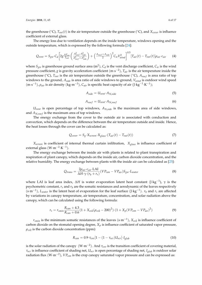
The energy loss due to ventilation depends on the inside temperature, windows opening and theoutside temperature, which is expressed by the following formula [24]:

Qvent = Sgw·Cd

[2g ∆Tair

Tout

(A2

roo f ·A2side

A2roo f +A2

side

)+( Aroo f +Aside

2

)2CwV2

wind

]0.5[Tair(t)− Tout(t)]ρair·cair (4)

where Sgw is greenhouse ground surface area (m2), Cd is the vent discharge coefficient, Cw is the windpressure coefficient, g is gravity acceleration coefficient (m·s−2), Tair is the air temperature inside thegreenhouse (◦C), Tout is the air temperature outside the greenhouse (◦C), Aroo f is area ratio of topwindows to the ground, Aside is area ratio of side windows to ground, Vwind is outdoor wind speed(m·s−1), ρair is air density (kg·m−3), Cair is specific heat capacity of air (J·kg−1·K−1);

Aside = Uvent·AN,side (5)

Aroo f = Uvent·AN,roo f (6)

Uvent is open percentage of top windows, AN,side is the maximum area of side windows,and AN,roo f is the maximum area of top windows.

The energy exchange from the cover to the outside air is associated with conduction andconvection, which depends on the difference between the air temperature outside and inside. Hence,the heat losses through the cover can be calculated as:

Qcover = Sg·Xscreen·Xglass·(Tair(t)− Tout(t)) (7)

Xscreen is coefficient of internal thermal curtain infiltration, Xglass is influence coefficient ofexternal glass (W·m−2·K−1).

The energy exchange between the inside air with plants is related to plant transpiration andrespiration of plant canopy, which depends on the inside air, carbon dioxide concentration, and therelative humidity. The energy exchange between plants with the inside air can be calculated as [25]:

Qtrans =2ρair·cair·LAI

∆H·γ·(rb + rs)(VPcan −VPair)Sgw·Lwater (8)

where LAI is leaf area index, ∆H is water evaporation latent heat constant (J·kg−1), γ is thepsychometric constant, rs and rb are the somatic resistances and aerodynamic of the leaves respectively(s·m−1), Lwater is the latent heat of evaporation for the leaf surface (J·kg−1). rb and rs are affectedby variations in canopy temperature, air temperature, concentration, and solar radiation above thecanopy, which can be calculated using the following formula:

rs = rsminRcan + 4.3Rcan + 0.6

(1 + Xco2(ρco2 − 200)2)·(1 + Xp(VPcan −VPair)2) (9)

rsmin is the minimum somatic resistances of the leaves (s·m−1), Xco2 is influence coefficient ofcarbon dioxide on the stomatal opening degree, Xp is influence coefficient of saturated vapor pressure,ρco2 is the carbon dioxide concentration (ppm):

Rcan = 0.9·τcov[1− (1− τscr)Uscr]·Iglob (10)

is the solar radiation of the canopy (W·m−2). And τcov is the transition coefficient of covering material,τscr is influence coefficient of shading net, Uscr is open percentage of shading net, Iglob is outdoor solarradiation flux (W·m−2), VPcan is the crop canopy saturated vapor pressure and can be expressed as:

Energies 2018, 11, 65 5 of 17

VPcan = 2.229× 1011·e5385

Tcan+273.15 (11)

where Tcan is the temperature of crop canopy, VPair can be expressed as:

VPair =Hair·R·(Tair + 273.15)

MH2O× 10−3 (12)

where R is the molar gas constant (J·kmol−1·K−1), Hair is the relative humidity, and MH2O is the molarmass of water (kg·kmol−1).

Heat flux of air is expressed by the temperature difference between inside air in time of t and timeof t − 1, which can be expressed as:

Qair = ρair·vg·cair·Tair(t)− Tair(t− 1)

∆t. (13)

where vg is greenhouse volume (m3), Tair(t) is the temperature at time t (◦C), and ∆t is the differencein time between t and t − 1, with a value of 300 (s).

Heat transfer from plant to greenhouse air depending on the difference between inside air andplant canopy can be calculated as:

Qcrop = 2Sgw·LAI·ρair·cair[Tair(t)− Tlea f (t)]

rb(14)

The solar radiation that penetrates the greenhouse cover is added into the greenhouse, and theenergy absorbed by the greenhouse can be expressed as:

Qsolar = Sg·0.9·τcov[1− (1− τscr)Uscr]·Iglob (15)

where Iglob is the outdoor radiation (W·m−2).The parameters in the mathematical model are analyzed according to the measured environmental

parameters and energy consumption values inside and outside the greenhouse. Then, the parametersin the model are divided into constant and uncertain parameters. The constant parameters in themodel are shown in Table 1.

Table 1. Constant physical parameters in a greenhouse model.

Parameters Physical Meaning Value Unit

LAI Leaf area index 2 m2·m−2

Sg Greenhouse cover surface area 1842 m2

K Stefan–Boltzmann constant 5.67× 10−8 W·m−2·K−4

g Gravity acceleration 9.8 m·s−2

AN,side Maximum area of side windows 0.10 m2·m−2

AN,roof Maximum area of top windows 0.18 m2·m−2

ρair Air density 1.2 kg·m−3

cair Specific heat capacity of air 1008 J·kg−1·K−1

∆H Water evaporation latent heat constant 2.45× 106 J·kg−1

γ Psychometric constant 65.8 Pa·KSgw Greenhouse ground surface area 912 m2

rsmin Minimum somatic resistances of the leaves 82 s·m−1

Lwater Latent heat of evaporation for the leaf surface 2.45× 106 J·kg−1

MH2O Molar mass of water 18 kg·kmol−1

R Molar gas constant 8314 J·kmol−1·K−1

νg Greenhouse volume 6840 m−3

rb Aerodynamic resistances of the leaves 275 s·m−1

ρwater Water density 1000 kg·m−3

cwater Specific heat capacity of water 4200 J·kg−1·◦C−1

Energies 2018, 11, 65 6 of 17

2.3. Method of Optimizing Parameters

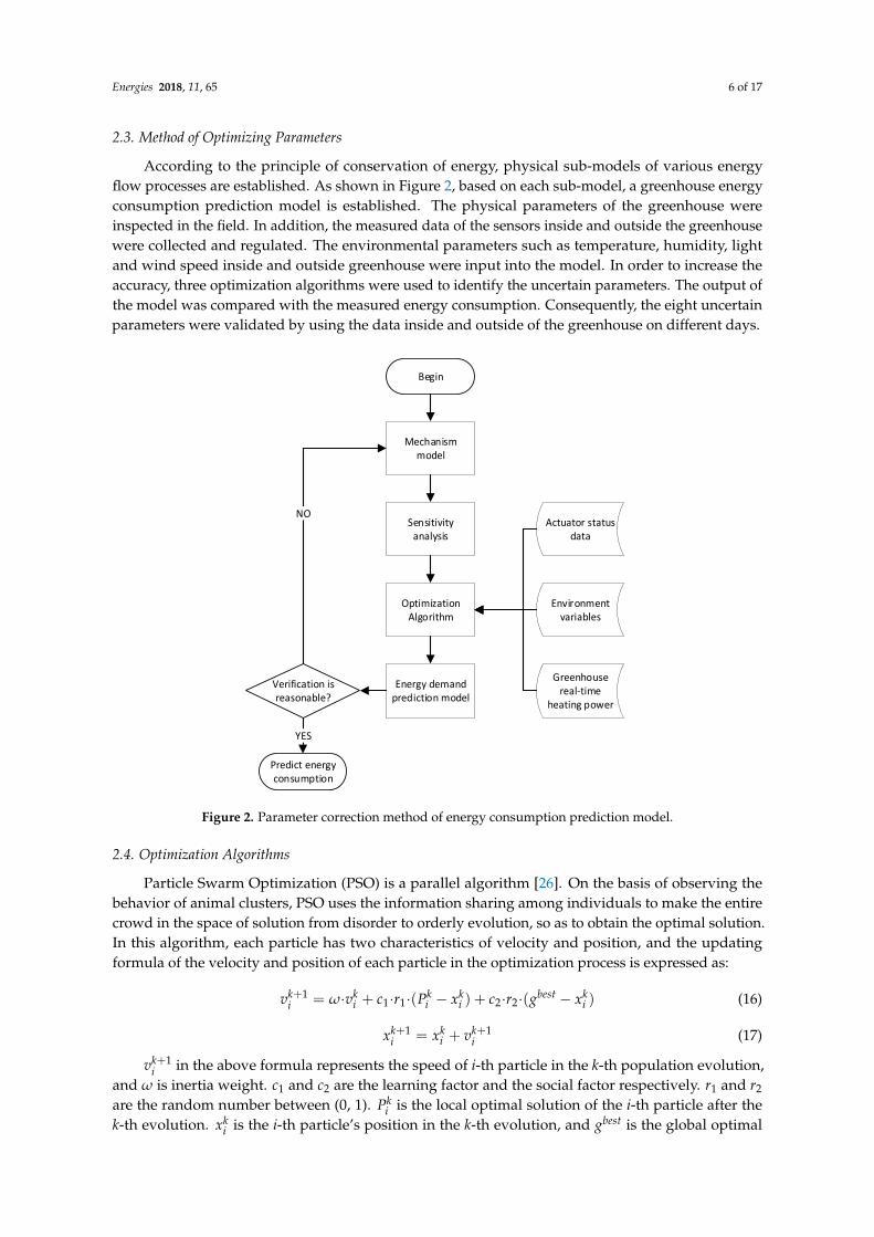
According to the principle of conservation of energy, physical sub-models of various energyflow processes are established. As shown in Figure 2, based on each sub-model, a greenhouse energyconsumption prediction model is established. The physical parameters of the greenhouse wereinspected in the field. In addition, the measured data of the sensors inside and outside the greenhousewere collected and regulated. The environmental parameters such as temperature, humidity, lightand wind speed inside and outside greenhouse were input into the model. In order to increase theaccuracy, three optimization algorithms were used to identify the uncertain parameters. The output ofthe model was compared with the measured energy consumption. Consequently, the eight uncertainparameters were validated by using the data inside and outside of the greenhouse on different days.

Energies 2018, 11, 65 6 of 17

uncertain parameters were validated by using the data inside and outside of the greenhouse on different days.

Begin

Mechanism model

Sensitivity analysis

OptimizationAlgorithm

Environment variables

Actuator status data

Verification is reasonable?

Energy demand prediction model

Predict energy consumption

YES

NO

Greenhouse real-time

heating power

Figure 2. Parameter correction method of energy consumption prediction model.

2.4. Optimization Algorithms

Particle Swarm Optimization (PSO) is a parallel algorithm [26]. On the basis of observing the behavior of animal clusters, PSO uses the information sharing among individuals to make the entire crowd in the space of solution from disorder to orderly evolution, so as to obtain the optimal solution. In this algorithm, each particle has two characteristics of velocity and position, and the updating formula of the velocity and position of each particle in the optimization process is expressed as: = ∙ + ∙ ∙ − + ∙ ∙ − (16) = + (17)

in the above formula represents the speed of i-th particle in the k-th population evolution, and is inertia weight. and are the learning factor and the social factor respectively. and are the random number between (0, 1). is the local optimal solution of the i-th particle after the k-th evolution. is the i-th particle’s position in the k-th evolution, and is the global optimal solution. PSO presents a series of characteristics that makes it the first choice in the algorithm selection for this research:

PSO has a real valued representation that allows avoiding the conversion to binary field and backwards, which is common in many heuristic algorithms.

PSO presents a swarm behavior, which is a sufficient approach in search spaces of considerable extension, due to the capability of exploration in steps of different lengths and the communication between particles, which share the information of the best results.

PSO is well known, therefore, there exists many publications about it, and numerous variations have already been proposed, in order to tackle problems of considerable complexity. In addition, there are already a lot of references about PSO calibration and stability.

Figure 2. Parameter correction method of energy consumption prediction model.

2.4. Optimization Algorithms

Particle Swarm Optimization (PSO) is a parallel algorithm [26]. On the basis of observing thebehavior of animal clusters, PSO uses the information sharing among individuals to make the entirecrowd in the space of solution from disorder to orderly evolution, so as to obtain the optimal solution.In this algorithm, each particle has two characteristics of velocity and position, and the updatingformula of the velocity and position of each particle in the optimization process is expressed as:

vk+1i = ω·vk

i + c1·r1·(Pki − xk

i ) + c2·r2·(gbest − xki ) (16)

xk+1i = xk

i + vk+1i (17)

vk+1i in the above formula represents the speed of i-th particle in the k-th population evolution,

and ω is inertia weight. c1 and c2 are the learning factor and the social factor respectively. r1 and r2

are the random number between (0, 1). Pki is the local optimal solution of the i-th particle after the

k-th evolution. xki is the i-th particle’s position in the k-th evolution, and gbest is the global optimal

Energies 2018, 11, 65 7 of 17

solution. PSO presents a series of characteristics that makes it the first choice in the algorithm selectionfor this research:

• PSO has a real valued representation that allows avoiding the conversion to binary field andbackwards, which is common in many heuristic algorithms.

• PSO presents a swarm behavior, which is a sufficient approach in search spaces of considerableextension, due to the capability of exploration in steps of different lengths and the communicationbetween particles, which share the information of the best results.

• PSO is well known, therefore, there exists many publications about it, and numerous variationshave already been proposed, in order to tackle problems of considerable complexity. In addition,there are already a lot of references about PSO calibration and stability.

Differential evolution algorithm (DE) [27], like PSO, as described in [28], is a computationalalgorithm based on the manipulation of a population of candidate solutions, applicable for complexsearch problems. It presents a series of interactions between the candidate solutions to produce newindividuals, and such new members are tested and catalogued by a cost function, seeking for thesurvival of only the ones with the best performance. The characteristics that makes it a suitable optionare enlisted below:

• DE is recognized as a greedy search algorithm. This marks the difference between the PSO andthe DE, and allows to check whether the group behavior is better than the greedy search in thequestions raised in this study.

• DE requires only two calibration factors, and the definition of these factors is quite small. Thisdefines DE as a simple calibration algorithm.

Genetic algorithm (GA) [29], in the reference [30], is used to simulate natural selection andnatural genetic process of reproduction, mating and mutation, one by one to produce the preferredindividuals, and finally get the best individual. Genetic algorithm is also an adaptive search algorithm,its selection, crossover, mutation and other operations are carried out in the form of probability, thereis a good global optimization and solving skills. The characteristics that makes it a suitable option arelisted below:

• Genetic algorithms are often used to generate high-quality solutions to optimize and search forproblems, relying on bio-inspired operators such as crossover, mutation and selection.

• Genetic algorithm simultaneously treats multiple individuals in a group, that is, evaluates multiplesolutions in the search space, reduces the risk of falling into the local optimal solution, andsimultaneously the algorithm itself is easy to realize parallelization.

According to the output of the energy consumption prediction model Qheat and the actual energyconsumption Qwater, the objective function is formulated as follows.

fi =

√1n ∑n

t=1 [Qheat(t)−Qwater(t)]2 (18)

Actually, the objective function means root-mean-square error (RMSE) in mathematics. Eachindividual is represented by a vector X = [ε, Xcover, Cd, Cw, Xscreen, Xglass, τcov, τscr], whereε, Xcover, Cd, Cw, Xscreen, Xglass, τcov and τscr have been mentioned before. The ranges of theseparameters are given in Table 2. Here, we use PSO as a representative to describe the whole proceduresof our proposed algorithms, as shown by Algorithm 1. Afterwards, the steps of three algorithms canbe summarized as follows.

Energies 2018, 11, 65 8 of 17

Algorithm 1: Outline. Steps of three algorithms in optimization.

Input: The environmental data: Tair, Tout, Aroo f , Vwind, ρco2, Uscr, Iglob, Tin, Topt, Uvent, HairOutput: The best vector (solution): ε, Xcover, Cd, Cw, Xscreen, Xglass, τcov, τscr

Step 1: Initialize the parameters of PSO such as ω, c1, c2, population size N, and the total generations Gen.Randomly initialize the velocity and position of the population, generating M vectors as N1, N2, . . . . . . ,XN. Set the initial iteration number gen = 0.

Step 2: Calculate the objective functions of the initial population according to Equation (18), where the valuesof Qheat and Qwater are computed from the input environment data as described in Section 2.2.

Step 3: Execute the PSO algorithm to perform the optimization procedure. Each individual is updatedaccording to Equations (16) and (17), and then compute the objective function. Afterwards, the globaloptimal solution Gbest for the population and the current optimal solution Pbest for each individualis updated.

Step 4: Update gen = gen + 1, if gen < Gen, go to step3, else stop.

The common parameters of the above three algorithms are given as the same values such aspopulation size and the total generations, while the calibration factors and updating mechanism are setup respectively. If DE and GA are utilized to perform the optimization process, only Step 1 and Step 3of Algorithm 1 need to be adjusted. For Step 1, some parameters with respect to these two algorithmsshould be set instead of those for PSO. While for Step 3, PSO is replaced by DE or GA, accordingly, thepopulation is evolved to a better condition in the objective space and a global optimal solution Gbest isgenerated in each generation.

3. Results and Discussion

3.1. Optimization and Validation

For the computational implementation, the deployed equipment is an Intel® CoreTM i7-2630QM,with a 2.00 GHZ processor and 8.00 GB in RAM, DDR3 1333 MHz type; the OS of the computer isWindowsTM 10 Professional Edition, and the machine is also equipped with the MATLABTM R2015aversion software.

For the three algorithms, population size N, and the total generations Gen are respectively setas 50 and 2000. The parameters of PSO such as ω, c1, and c2 are respectively set as 0.9, 0.12 and 1.2.For the DE algorithm, the scaling factor F and the crossover probability Cr are respectively set as 0.5and 0.9. For the GA algorithm, the crossover and mutation probabilities are 0.8 and 0.1 respectively.Moreover, the simulated binary crossover (SBX) and polynomial mutation operators are used togenerate offspring solutions, where the distribution factors in are both 20.

According to the prediction model of the energy consumption and three optimization algorithms,we write the program of Matlab and identify the uncertain parameters in the parametric model.The obtained results of parameters by each algorithm are shown in Table 2. It should be noted thatcalibration parameters, like in the other algorithms, were selected experimentally, based on the bestresults obtained after several tests.

Table 2. The optimized parameters results with three algorithms.

Parameters Range GA DE PSO

ε [0.5, 0.8] 0.55 0.61 0.65Xcover [0.1, 0.9] 0.43 0.27 0.33

Cd [0.6, 0.8] 0.71 0.74 0.77Cw [0.05, 0.2] 0.15 0.11 0.12

Xscreen [0.3, 0.9] 0.49 0.52 0.55Xglass [1, 10] 5.79 6.23 5.19τcov [0.6, 1] 0.63 0.77 0.83τscr [0.3, 0.9] 0.72 0.87 0.71

Energies 2018, 11, 65 9 of 17

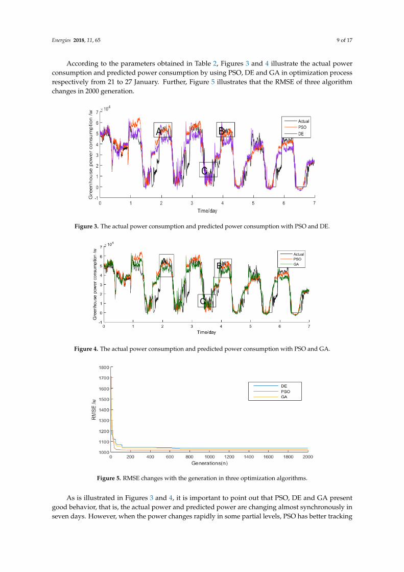
According to the parameters obtained in Table 2, Figures 3 and 4 illustrate the actual powerconsumption and predicted power consumption by using PSO, DE and GA in optimization processrespectively from 21 to 27 January. Further, Figure 5 illustrates that the RMSE of three algorithmchanges in 2000 generation.Energies 2018, 11, 65 9 of 17

Figure 3. The actual power consumption and predicted power consumption with PSO and DE.

Figure 4. The actual power consumption and predicted power consumption with PSO and GA.

Figure 5. RMSE changes with the generation in three optimization algorithms.

As is illustrated in Figures 3 and 4, it is important to point out that PSO, DE and GA present good behavior, that is, the actual power and predicted power are changing almost synchronously in seven days. However, when the power changes rapidly in some partial levels, PSO has better tracking results than GA and DE, such as A, B, C. In real greenhouses, tracking of short-term power changes is very important because of the rapidly changing weather. Figure 5 shows RMSE changes with the generation in three optimization algorithms and it illustrates that when PSO runs to 87 generations, it completely converges, while GA and DE converge locally at 120 generations, then jump to local convergence at 600 generations and 700 generations respectively, which shows the global search ability of GA and DE. However, the PSO converges faster, and RSME is less than GA and DE.

According to the parameters obtained by the PSO optimization algorithm, the energy consumption prediction model is obtained. In order to check the model, the actual data of the five days from February 1 to 5 February 2016 is used for verification.

Figure 3. The actual power consumption and predicted power consumption with PSO and DE.

Energies 2018, 11, 65 9 of 17

Figure 3. The actual power consumption and predicted power consumption with PSO and DE.

Figure 4. The actual power consumption and predicted power consumption with PSO and GA.

Figure 5. RMSE changes with the generation in three optimization algorithms.

As is illustrated in Figures 3 and 4, it is important to point out that PSO, DE and GA present good behavior, that is, the actual power and predicted power are changing almost synchronously in seven days. However, when the power changes rapidly in some partial levels, PSO has better tracking results than GA and DE, such as A, B, C. In real greenhouses, tracking of short-term power changes is very important because of the rapidly changing weather. Figure 5 shows RMSE changes with the generation in three optimization algorithms and it illustrates that when PSO runs to 87 generations, it completely converges, while GA and DE converge locally at 120 generations, then jump to local convergence at 600 generations and 700 generations respectively, which shows the global search ability of GA and DE. However, the PSO converges faster, and RSME is less than GA and DE.

According to the parameters obtained by the PSO optimization algorithm, the energy consumption prediction model is obtained. In order to check the model, the actual data of the five days from February 1 to 5 February 2016 is used for verification.

Figure 4. The actual power consumption and predicted power consumption with PSO and GA.

Energies 2018, 11, 65 9 of 17

Figure 3. The actual power consumption and predicted power consumption with PSO and DE.

Figure 4. The actual power consumption and predicted power consumption with PSO and GA.

Figure 5. RMSE changes with the generation in three optimization algorithms.

As is illustrated in Figures 3 and 4, it is important to point out that PSO, DE and GA present good behavior, that is, the actual power and predicted power are changing almost synchronously in seven days. However, when the power changes rapidly in some partial levels, PSO has better tracking results than GA and DE, such as A, B, C. In real greenhouses, tracking of short-term power changes is very important because of the rapidly changing weather. Figure 5 shows RMSE changes with the generation in three optimization algorithms and it illustrates that when PSO runs to 87 generations, it completely converges, while GA and DE converge locally at 120 generations, then jump to local convergence at 600 generations and 700 generations respectively, which shows the global search ability of GA and DE. However, the PSO converges faster, and RSME is less than GA and DE.

According to the parameters obtained by the PSO optimization algorithm, the energy consumption prediction model is obtained. In order to check the model, the actual data of the five days from February 1 to 5 February 2016 is used for verification.

Figure 5. RMSE changes with the generation in three optimization algorithms.

As is illustrated in Figures 3 and 4, it is important to point out that PSO, DE and GA presentgood behavior, that is, the actual power and predicted power are changing almost synchronously inseven days. However, when the power changes rapidly in some partial levels, PSO has better tracking

Energies 2018, 11, 65 10 of 17

results than GA and DE, such as A, B, C. In real greenhouses, tracking of short-term power changesis very important because of the rapidly changing weather. Figure 5 shows RMSE changes with thegeneration in three optimization algorithms and it illustrates that when PSO runs to 87 generations,it completely converges, while GA and DE converge locally at 120 generations, then jump to localconvergence at 600 generations and 700 generations respectively, which shows the global search abilityof GA and DE. However, the PSO converges faster, and RSME is less than GA and DE.

According to the parameters obtained by the PSO optimization algorithm, the energy consumptionprediction model is obtained. In order to check the model, the actual data of the five days from February1 to 5 February 2016 is used for verification.

As shown in Figure 6, the predicted power consumption meets the actual power well in general.There is also some difference between predicted and actual power consumption, especially during thenoon when heating system fluctuates more than usual. Finally, the daily energy consumption errorwas 7.42% and the model shows good robustness.

Energies 2018, 11, 65 10 of 17

As shown in Figure 6, the predicted power consumption meets the actual power well in general. There is also some difference between predicted and actual power consumption, especially during the noon when heating system fluctuates more than usual. Finally, the daily energy consumption error was 7.42% and the model shows good robustness.

Figure 6. The actual power consumption and predicted power consumption with PSO in verification.

Table 3 describes the relative errors between the predicted and the actual power consumption which are measured from 6 to 15 February. When the greenhouse average daily solar radiation is between 160 (W ∙ m ) and 270 (W ∙ m ), and the outdoor average temperature is between 3–5 (°C), the error of predicted power consumption is less than 11%. Consequently, when the daily average light and the outdoor average temperature change are small, the model shows a good performance for prediction of short-term greenhouse energy consumption.

Table 3. The relative errors between actual consumption and predicted consumption.

Date (yy-mm-dd)

Outdoor Average Light ( ∙ )

Outdoor Average Temperature (°C)

Average Power (kW)

Relative Error (%)

2016-02-06 167.1354 3.30 31.32 9.12 2016-02-07 210.3487 3.73 33.45 8.34 2016-02-08 223.9821 3.90 32.83 7.71 2016-02-09 218.6615 3.88 33.21 6.21 2016-02-10 228.4269 4.03 31.58 5.19 2016-02-11 245.5491 4.56 27.48 10.13 2016-02-12 230.4658 4.13 30.44 9.33 2016-02-13 248.5611 4.63 26.55 10.42 2016-02-14 270.4660 5.01 21.12 10.57 2016-02-15 297.4558 5.95 17.43 10.85

3.2. Predict Energy Consumption Based on Model

In winter, normal greenhouse production requires efficient management of energy consumption. According to statistics, heating costs in winter greenhouse can reach more than 50% of greenhouse production costs [31]. As the accuracy of weather forecasting model increases, the prediction of the outdoor environment change is more reliable. Therefore, the accuracy of the temperature, light and wind speed has been guaranteed. At present, the outdoor weather data in one week can already be used to manage the greenhouse of heating production.

Taking the Chongming greenhouse as an example in this study, energy-related devices include top windows, external shading net, internal thermal curtain and internal shading net. From January to March, it is the coldest season of one year. In this period of time, these devices have some rules to follow, which are shown in Figure 7.

Figure 6. The actual power consumption and predicted power consumption with PSO in verification.

Table 3 describes the relative errors between the predicted and the actual power consumptionwhich are measured from 6 to 15 February. When the greenhouse average daily solar radiation isbetween 160 (W·m−2) and 270 (W·m−2), and the outdoor average temperature is between 3–5 (◦C),the error of predicted power consumption is less than 11%. Consequently, when the daily averagelight and the outdoor average temperature change are small, the model shows a good performance forprediction of short-term greenhouse energy consumption.

Table 3. The relative errors between actual consumption and predicted consumption.

Date (yy-mm-dd) Outdoor AverageLight (W·m−2)

Outdoor AverageTemperature (◦C)

Average Power(kW) Relative Error (%)

2016-02-06 167.1354 3.30 31.32 9.122016-02-07 210.3487 3.73 33.45 8.342016-02-08 223.9821 3.90 32.83 7.712016-02-09 218.6615 3.88 33.21 6.212016-02-10 228.4269 4.03 31.58 5.192016-02-11 245.5491 4.56 27.48 10.132016-02-12 230.4658 4.13 30.44 9.332016-02-13 248.5611 4.63 26.55 10.422016-02-14 270.4660 5.01 21.12 10.572016-02-15 297.4558 5.95 17.43 10.85

Energies 2018, 11, 65 11 of 17

3.2. Predict Energy Consumption Based on Model

In winter, normal greenhouse production requires efficient management of energy consumption.According to statistics, heating costs in winter greenhouse can reach more than 50% of greenhouseproduction costs [31]. As the accuracy of weather forecasting model increases, the prediction of theoutdoor environment change is more reliable. Therefore, the accuracy of the temperature, light andwind speed has been guaranteed. At present, the outdoor weather data in one week can already beused to manage the greenhouse of heating production.

Taking the Chongming greenhouse as an example in this study, energy-related devices includetop windows, external shading net, internal thermal curtain and internal shading net. From Januaryto March, it is the coldest season of one year. In this period of time, these devices have some rules tofollow, which are shown in Figure 7.Energies 2018, 11, 65 11 of 17

Figure 7. The open degree of execution agents.

For example, at about 1 o’clock p.m., the top windows usually open for about two hours. At this time, the temperature is in the highest stage in the day, and the temperature in the room rises sharply. Thus, opening the top windows and the shading net helps to discharge excess heat in the greenhouse. As a result, heat transfer from heat pump to the greenhouse will be close to zero.

It can be seen that the greenhouse will not be heated when the shade net and the top windows are opened. When the greenhouse absorbs redundant energy, the power output resulting from the prediction model is negative and excess energy is released through the opening of top windows and the shade net. Therefore, to ensure the decrease of inside temperature, the output power of heat pump is kept as zero. In the night (7:00 p.m. to 8:00 a.m.) in order to resist the outdoor cold, the internal insulation is open, while the shade net is also open because the shading net could decrease the heat loss from the greenhouse to outside.

As shown in Figures 8 and 9, from January 23 to January 27, the actual indoor and outdoor temperature, and light in the Chongming greenhouse change slowly. Furthermore, they follow the trend of first rising and then falling during a day.

Therefore, in daily management of greenhouses, based on the day’s outdoor temperature and indoor temperature trends from 23 to 27 January, the given average outdoor temperature and solar radiation can be converted into the same time series. According to the prediction model of energy consumption in greenhouse, the indoor daily average temperature is fixed at 22 °C, and the daily total energy consumption of greenhouse is predicted with different outdoor average temperature and light, as shown in Figure 10.

Figure 8. The temperature trends over time.

Figure 7. The open degree of execution agents.

For example, at about 1 o’clock p.m., the top windows usually open for about two hours. At thistime, the temperature is in the highest stage in the day, and the temperature in the room rises sharply.Thus, opening the top windows and the shading net helps to discharge excess heat in the greenhouse.As a result, heat transfer from heat pump to the greenhouse will be close to zero.

It can be seen that the greenhouse will not be heated when the shade net and the top windowsare opened. When the greenhouse absorbs redundant energy, the power output resulting from theprediction model is negative and excess energy is released through the opening of top windows andthe shade net. Therefore, to ensure the decrease of inside temperature, the output power of heat pumpis kept as zero. In the night (7:00 p.m. to 8:00 a.m.) in order to resist the outdoor cold, the internalinsulation is open, while the shade net is also open because the shading net could decrease the heatloss from the greenhouse to outside.

As shown in Figures 8 and 9, from January 23 to January 27, the actual indoor and outdoortemperature, and light in the Chongming greenhouse change slowly. Furthermore, they follow thetrend of first rising and then falling during a day.

Therefore, in daily management of greenhouses, based on the day’s outdoor temperature andindoor temperature trends from 23 to 27 January, the given average outdoor temperature and solarradiation can be converted into the same time series. According to the prediction model of energyconsumption in greenhouse, the indoor daily average temperature is fixed at 22 ◦C, and the daily totalenergy consumption of greenhouse is predicted with different outdoor average temperature and light,as shown in Figure 10.

Energies 2018, 11, 65 12 of 17

Energies 2018, 11, 65 11 of 17

Figure 7. The open degree of execution agents.

For example, at about 1 o’clock p.m., the top windows usually open for about two hours. At this time, the temperature is in the highest stage in the day, and the temperature in the room rises sharply. Thus, opening the top windows and the shading net helps to discharge excess heat in the greenhouse. As a result, heat transfer from heat pump to the greenhouse will be close to zero.

It can be seen that the greenhouse will not be heated when the shade net and the top windows are opened. When the greenhouse absorbs redundant energy, the power output resulting from the prediction model is negative and excess energy is released through the opening of top windows and the shade net. Therefore, to ensure the decrease of inside temperature, the output power of heat pump is kept as zero. In the night (7:00 p.m. to 8:00 a.m.) in order to resist the outdoor cold, the internal insulation is open, while the shade net is also open because the shading net could decrease the heat loss from the greenhouse to outside.

As shown in Figures 8 and 9, from January 23 to January 27, the actual indoor and outdoor temperature, and light in the Chongming greenhouse change slowly. Furthermore, they follow the trend of first rising and then falling during a day.

Therefore, in daily management of greenhouses, based on the day’s outdoor temperature and indoor temperature trends from 23 to 27 January, the given average outdoor temperature and solar radiation can be converted into the same time series. According to the prediction model of energy consumption in greenhouse, the indoor daily average temperature is fixed at 22 °C, and the daily total energy consumption of greenhouse is predicted with different outdoor average temperature and light, as shown in Figure 10.

Figure 8. The temperature trends over time. Figure 8. The temperature trends over time.Energies 2018, 11, 65 12 of 17

Figure 9. The light trends over time.

Figure 10. The predicted daily energy consumption under different outdoor temperature and solar radiation.

When we fix the average daily outdoor solar radiation at 200 W/m , the daily total energy consumption of greenhouse is predicted according to different outdoor average temperature and indoor average temperature, as shown in Figure 11.

Figure 11. The predicted daily energy consumption under different outdoor temperature and indoor temperature.

When the outdoor average temperature is constant, the total daily energy consumption decreases with the increase of the total solar radiation. Similarly, based on the given constant solar radiation, the total daily energy consumption also decreases with the increase of the outdoor average temperature. If the outdoor temperature and light are the same, the daily total energy consumption increases with rising of the indoor temperature. These reasonable results can provide guidance for management of the greenhouse.

Figure 9. The light trends over time.

Energies 2018, 11, 65 12 of 17

Figure 9. The light trends over time.

Figure 10. The predicted daily energy consumption under different outdoor temperature and solar radiation.

When we fix the average daily outdoor solar radiation at 200 W/m , the daily total energy consumption of greenhouse is predicted according to different outdoor average temperature and indoor average temperature, as shown in Figure 11.

Figure 11. The predicted daily energy consumption under different outdoor temperature and indoor temperature.

When the outdoor average temperature is constant, the total daily energy consumption decreases with the increase of the total solar radiation. Similarly, based on the given constant solar radiation, the total daily energy consumption also decreases with the increase of the outdoor average temperature. If the outdoor temperature and light are the same, the daily total energy consumption increases with rising of the indoor temperature. These reasonable results can provide guidance for management of the greenhouse.

Figure 10. The predicted daily energy consumption under different outdoor temperature andsolar radiation.

When we fix the average daily outdoor solar radiation at 200 W/m2, the daily total energyconsumption of greenhouse is predicted according to different outdoor average temperature andindoor average temperature, as shown in Figure 11.

Energies 2018, 11, 65 13 of 17

Energies 2018, 11, 65 12 of 17

Figure 9. The light trends over time.

Figure 10. The predicted daily energy consumption under different outdoor temperature and solar radiation.

When we fix the average daily outdoor solar radiation at 200 W/m , the daily total energy consumption of greenhouse is predicted according to different outdoor average temperature and indoor average temperature, as shown in Figure 11.

Figure 11. The predicted daily energy consumption under different outdoor temperature and indoor temperature.

When the outdoor average temperature is constant, the total daily energy consumption decreases with the increase of the total solar radiation. Similarly, based on the given constant solar radiation, the total daily energy consumption also decreases with the increase of the outdoor average temperature. If the outdoor temperature and light are the same, the daily total energy consumption increases with rising of the indoor temperature. These reasonable results can provide guidance for management of the greenhouse.

Figure 11. The predicted daily energy consumption under different outdoor temperature andindoor temperature.

When the outdoor average temperature is constant, the total daily energy consumption decreaseswith the increase of the total solar radiation. Similarly, based on the given constant solar radiation, thetotal daily energy consumption also decreases with the increase of the outdoor average temperature.If the outdoor temperature and light are the same, the daily total energy consumption increases withrising of the indoor temperature. These reasonable results can provide guidance for management ofthe greenhouse.

3.3. Optimization of Daily Average Temperature

At different growth stages, crops’ requirements from the environment are an average amount.For example, the temperature requirement is in the form of accumulated temperature as long asinstantaneous value is not too high or too low to damage the crop. Normally, the same accumulatedtemperature can resulted in the same yield for many crops [32–34]. In order to manage the greenhouseand realize the maximum profit, the energy consumption must be planned and optimized to dealwith the changeable weather. Since crop growth stage is still a long time, crops’ one week averagetemperature requirement can be considered as constant through the planting cycle. In the greenhouse,when the average temperature of a week is given as constant, the daily average temperature still needsto be optimized according to the outdoor weather. The reason is that weather changes are complicatedand extreme weather conditions such as cold waves may occur in a week. Compared with normalclimatic conditions, achieving the same temperature setting consumes more energy in a cold waveperiod. Therefore, it is significant to optimize daily temperature under the given condition of weeklyaverage temperature.

3.3.1. Energy Optimization Algorithm Objective Function

In this study, the heating system of the Chongming greenhouse uses hot water pipes for heating,which accounts for more than 90% of the production costs in winter. According to the energyconsumption prediction model analyzed in the previous chapter, the objective function of energyconsumption for optimizing the daily average temperature is as follows:

Min:

J(x) =7

∑i=7

(Qheat(TDi)) x = [TD1, TD2, TD3, TD4, TD5, TD6, TD7] (19)

subject to:∑7

i=7 TDi

7= Tweek Tmin < TDi < Tmax (i = 1, 2, . . . , 7) (20)

Among them, the objective function J(x) represents the total energy consumption of one weekwith different daily average temperatures. Qheat(TDi) represents the energy consumption prediction

Energies 2018, 11, 65 14 of 17

model obtained in the previous section, and x = [TD1, TD2, TD3, TD4, TD5, TD6, TD7] represents sevendaily average temperatures. The equation constraint Tweek is according to historical planting experienceand crops growth characteristics. Tmin and Tmax represent the appropriate crop temperature range.

3.3.2. Optimization Process of Daily Average Temperature

Based on the accumulated temperature theory which has been mentioned before, thesingle-objective particle swarm optimization is used to optimize the daily average temperature, whereone-week energy consumption is used as performance index, the average temperature of one weekand each day are used as constraints to optimize the daily average temperatures. Corresponding tothe lowest cost, the daily average temperatures are selected as the target setting values on the basis ofmeeting the above constraints.

In this paper, we use the average temperature under the control of the Chongming Priva systemas the given average weekly temperature. As the Priva system is a mature control system, it has goodeffect on a global scale. It can be considered that the control result is able to meet the requirements ofcrops for temperature accumulation. From 22 to 28 February, this stage is the tomato growing periodin the Chongming greenhouse, requiring a higher temperature during the day to 23–26 ◦C [23–25].Where the actual average temperature is 23.6 ◦C in one week, the best daily average temperature rangein greenhouse is 20–25 ◦C, and the allowable deviation range is 1 ◦C. Furthermore, 19 ◦C and 26 ◦C arethe lower and upper boundary of optimization variables.

As shown in Figure 12, the actual average daily temperature of the Chongming greenhouse meetsthe crop temperature requirements in a week. The daily average temperatures without optimizationremain stable in this week, however, as shown in Figure 12, from 25 to 27 February, the greenhouseexperiences a short-term cold wave, and the outdoor extreme temperature reaches below −9 (◦C).When compared with 24 February, heating the greenhouse to the same temperature will lose moreenergy due to the lower outdoor temperature.

Based on the optimization algorithm and weather forecast for one week, the daily averagetemperatures of 7 days are optimized. Consequently, in order to maintain the average temperatures of7 days meeting with the weekly average temperature constraints, the daily average temperatures areappropriately increased before and decreased after the arrival of cold wave respectively. It will help toavoid the loss of energy cost caused by the constant temperature heating during the coldest periodwhile ensuring the normal crop growth. The optimized seven-day average temperatures are verifiedby the energy consumption model in this paper.

Energies 2018, 11, 65 14 of 17

As shown in Figure 12, the actual average daily temperature of the Chongming greenhouse meets the crop temperature requirements in a week. The daily average temperatures without optimization remain stable in this week, however, as shown in Figure 12, from 25 to 27 February, the greenhouse experiences a short-term cold wave, and the outdoor extreme temperature reaches below −9 (°C). When compared with 24 February, heating the greenhouse to the same temperature will lose more energy due to the lower outdoor temperature.

Based on the optimization algorithm and weather forecast for one week, the daily average temperatures of 7 days are optimized. Consequently, in order to maintain the average temperatures of 7 days meeting with the weekly average temperature constraints, the daily average temperatures are appropriately increased before and decreased after the arrival of cold wave respectively. It will help to avoid the loss of energy cost caused by the constant temperature heating during the coldest period while ensuring the normal crop growth. The optimized seven-day average temperatures are verified by the energy consumption model in this paper.

Figure 12. The daily average temperature in one week of optimization.

3.4. Discussion

Taking again the Chongming greenhouse as an example in this study, we compare three classic algorithms to predict energy consumption. According to the parameters obtained by the best result, the greenhouse energy consumption prediction model is established. In order to verify the accuracy of the developed model, energy consumption from 6 to 15 February is predicted according to the greenhouse environmental data. The predicted energy consumption is almost in the same trend to the actual energy consumption, and the RMSE is less than 11%. Afterwards, the model shows a good performance for prediction of short-term greenhouse energy consumption.

Generally, the average temperature over a period of time is given according to the growth demand of crops. According to the outdoor weather forecast, the energy consumption at a given average temperature needs to be predicted to adjust the heating. However, the current studies on greenhouse energy consumption focus on proposing new algorithms to improve the accuracy of the model, ignoring the application of the model in practical situations. Uniquely, in this study, the energy consumption model is exploited for the real prediction of greenhouse energy consumption in actual production. Based on the law of energy-related devices and the outdoor weather forecasting, the daily average temperatures of 7 days are optimized during a cold wave. In terms of energy conservation, the optimized average temperatures save 9% of the energy cost, and provide considerable economic benefits in a greenhouse with a heating area of 1000 square meters. Compared

Figure 12. The daily average temperature in one week of optimization.

Energies 2018, 11, 65 15 of 17

3.4. Discussion

Taking again the Chongming greenhouse as an example in this study, we compare three classicalgorithms to predict energy consumption. According to the parameters obtained by the best result,the greenhouse energy consumption prediction model is established. In order to verify the accuracyof the developed model, energy consumption from 6 to 15 February is predicted according to thegreenhouse environmental data. The predicted energy consumption is almost in the same trend tothe actual energy consumption, and the RMSE is less than 11%. Afterwards, the model shows a goodperformance for prediction of short-term greenhouse energy consumption.

Generally, the average temperature over a period of time is given according to the growthdemand of crops. According to the outdoor weather forecast, the energy consumption at a givenaverage temperature needs to be predicted to adjust the heating. However, the current studies ongreenhouse energy consumption focus on proposing new algorithms to improve the accuracy of themodel, ignoring the application of the model in practical situations. Uniquely, in this study, the energyconsumption model is exploited for the real prediction of greenhouse energy consumption in actualproduction. Based on the law of energy-related devices and the outdoor weather forecasting, the dailyaverage temperatures of 7 days are optimized during a cold wave. In terms of energy conservation,the optimized average temperatures save 9% of the energy cost, and provide considerable economicbenefits in a greenhouse with a heating area of 1000 square meters. Compared with the previousresearch, this paper studies the use of energy consumption model in practical situations, and proposesthe concept of daily average temperature optimization for the first time.

4. Conclusions

Based on the analysis of energy exchange between the greenhouse and the outside world, themechanism model of a greenhouse is established. Combining the existing measured data withthe optimized algorithm, the parameters are identified by optimization algorithms. The energyconsumption prediction model of greenhouse is established, which provides reference for greenhouseenergy consumption optimization and management. The conclusions are as follows:

(1) The essence of temperature change is the result of various heat and mass transfer processes ingreenhouse. Therefore, based on the dynamic equations of these processes and thermodynamictheory, greenhouse energy consumption model is established.

(2) According to the analysis of the various parameters involved in the energy consumptionmodel, we determine the parameters to be identified and the energy consumption modelof the parameters to be calibrated. The measured data of greenhouse environment and thestates information of devices are input into the model. Also, three optimization algorithms areused to identify the uncertain parameters in the prediction model. Finally, five days after ofthe greenhouse environmental data is used to verify the effectiveness of energy consumptionprediction model.

(3) At present, the accuracy of the weather forecast in one week has been guaranteed. Based on crops’requirements on accumulated temperature theory, the energy consumption prediction model, theoptimized economy is obtained under the constraints of weekly average temperature and dailyaverage temperature. Optimizing the daily average temperature for one week can reasonablyguide the greenhouse heating production under the extreme weather conditions. As a result, theenergy consumption is reduced, and the normal crop growth is ensured. At the same time, theeconomic benefits of the greenhouse are improved.

This paper presents a greenhouse energy consumption prediction model for winter heatingoptimization. Combining with accumulated temperature theory, when the accuracy of the weatherforecast is guaranteed, the daily temperature averages will be optimized in the current week. Finally,good results have been obtained. However, the process of energy exchange in the greenhouse is

Energies 2018, 11, 65 16 of 17

complicated and the outdoor weather varies. The energy consumption prediction model is alsodifficult to be apply to the energy prediction in different seasons within about 365 days of the year.The energy consumption prediction model for cooling in summer still needs to be further studied.Similarly, subject to the accuracy of the weather forecast, the current greenhouse can be used tooptimize the daily average temperature with a given average temperature for one week. The furtheroptimization of the weekly average temperature remains to be studied.

Acknowledgments: This work was supported in part by the National High-Tech N & E Program of China underGrant 2013AA103006-2, the National Science Foundation of China under Grant 61573258, and in part by the U.S.National Science Foundation’s BEACON Center for the Study of Evolution in Action, funded under CooperativeAgreement #DBI-0939454.

Author Contributions: Yongtao Shen and Ruihua Wei conceived and designed the experiments. Yongtao Shenperformed the experiments. Ruihua Wei analyzed the data. Lihong Xu contributed materials/analysis tools.Yongtao Shen wrote the paper.

Conflicts of Interest: The authors declare no conflict of interest.

References

1. Hemming, S.; Balendonck, J.; Dieleman, J.A.; de Gelder, A.; Kempkes, F.L.K.; Swinkels, G.L.A.M.;de Visser, P.H.B.; de Zwart, H.F. Innovations in greenhouse systems—Energy conservation by system design,sensors and decision support systems. In Proceedings of the ISHS Acta Horticulturae 1170: InternationalSymposium on New Technologies and Management for Greenhouses—GreenSys 2015, Evora, Portugal,19–23 July 2015.

2. De Zwart, H.F. Analyzing Energy-Saving Options in Greenhouse Cultivation Using a Simulation Model; DOLInstitute of Agricultural and Environment: Wageningen, The Netherlands, 1996.

3. Gupta, M.J.; Chandra, P. Effect of greenhouse design parameters on conservation of energy for greenhouseenvironmental control. Energy 2002, 27, 777–794. [CrossRef]

4. Su, Y.; Xu, L.; Li, D. Adaptive fuzzy control of a class of MIMO nonlinear system with actuator saturation forgreenhouse climate control problem. IEEE Trans. Autom. Sci. Eng. 2016, 13, 772–788. [CrossRef]

5. Spanomitsios, G.K. SE—Structure and Environment: Temperature Control and Energy Conservation in aPlastic Greenhouse. J. Agric. Eng. Res. 2001, 80, 251–259. [CrossRef]

6. Dai, J.; Luo, W.; Li, Y. A microclimate model-based energy consumption prediction system for greenhouseheating. Sci. Agric. Sin. 2006, 11, 21.

7. Xu, F.; Zhang, L.; Chen, J.; Zhan, H. Modeling and simulation of subtropical greenhouse microclimate inChina. Trans. Chin. Soc. Agric. Mach. 2005, 36, 102–105.

8. Ren, S.; Yang, W.; Wang, H.; Xue, W.; Xu, H.; Xiong, Y. Prediction model on temporal and spatial variation ofair temperature in greenhouse and ventilation control measures based on CFD. Trans. Chin. Soc. Agric. Eng.2015, 31, 207–214.

9. Patil, S.L.; Tantau, H.J.; Salokhe, V.M. Modelling of tropical greenhouse temperature by auto regressive andneural network models. Biosyst. Eng. 2008, 99, 423–431. [CrossRef]

10. Ferreira, P.M.; Faria, E.A.; Ruano, A.E. Neural network models in greenhouse air temperature prediction.Neurocomputing 2002, 43, 51–75. [CrossRef]

11. Nabavi-Pelesaraei, A.; Abdi, R.; Rafiee, S. Neural network modeling of energy use and greenhouse gasemissions of watermelon production systems. J. Saudi Soc. Agric. Sci. 2016, 15, 38–47. [CrossRef]

12. Kavga, A.; Kappatos, V. Estimation of the Temperatures in an Experimental Infrared Heated GreenhouseUsing Neural Network Models. Int. J. Agric. Environ. Inf. Syst. 2017, 4, 14–22. [CrossRef]

13. Fourati, F. Multiple neural control of a greenhouse. Neurocomputing 2014, 139, 138–144. [CrossRef]14. Frausto, H.U.; Pieters, J.G. Modelling greenhouse temperature using system identification by means of

neural networks. Neurocomputing 2004, 56, 423–428. [CrossRef]15. Trejoperea, M.; Herreraruiz, G.; Riosmoreno, J.; Miranda, R.C. Greenhouse energy consumption prediction

using neural networks models. Int. J. Agric. Biol. 2009, 11, 1–6.16. Coelho, J.P.; Pbde, M.O.; Boaventura, C.J. Greenhouse air temperature predictive control using the particle

swarm optimisation algorithm. Comput. Electron. Agric. 2005, 49, 330–344. [CrossRef]

Energies 2018, 11, 65 17 of 17

17. Pérez-González, A.; Begovich, O.; Ruiz-León, J. Modeling of a greenhouse prototype using PSO algorithmbased on a LabViewTM application. In Proceedings of the 2014 11th International Conference on ElectricalEngineering, Computing Science and Automatic Control, Campeche, Mexico, 29 September–3 October 2014;pp. 1–6.

18. Hasni, A.; Taibi, R.; Draoui, B.; Boulard, T. Optimization of Greenhouse Climate Model Parameters UsingParticle Swarm Optimization and Genetic Algorithms. Energy Procedia 2011, 6, 371–380. [CrossRef]

19. Avila-Miranda, R.; Begovich, O.; Ruiz-León, J. An optimal and intelligent control strategy to ventilate agreenhouse. In Proceedings of the 2013 IEEE Congress on Evolutionary Computation, Cancun, Mexico,20–23 June 2013; pp. 779–782.

20. Chen, J.; Chen, J.; Yang, J.; Xu, F.; Zhen, S. Prediction on energy consumption of semi-closed greenhousesbased on self-accelerating PSO-GA. Trans. Chin. Soc. Agric. Eng. 2015, 31, 186–198.

21. Chen, J.; Yang, J.; Zhao, J.; Xu, F.; Zhen, S.; Zhang, L. Energy demand forecasting of the greenhouses usingnonlinear models based on model optimized prediction method. Neurocomputing 2016, 174, 1087–1100.[CrossRef]

22. Pérez-González, A.; Begovich-Mendoza, O.; Ruiz-León, J. Modeling of a greenhouse prototype using PSOand differential evolution algorithms based on a real-time LabView™ application. Appl. Soft Comput. 2018,62, 86–100. [CrossRef]

23. Eckel, D. Heat and Mass Transfer; Science Press: Beijing, China, 1963.24. Kittas, C.; Boulard, T.; Papadakis, G. Natural ventilation of a greenhouse with ridge and side openings:

Sensitivity to temperature and wind effects. Am. Soc. Agric. Biol. Eng. 1997, 40, 415–425. [CrossRef]25. Stanghellini, C.; Jong, T.D. A model of humidity and its applications in a greenhouse. Agric. For. Meteorol.

1995, 76, 129–148. [CrossRef]26. Juang, C.F.; Liou, Y.C. On the hybrid of genetic algorithm and particle swarm optimization for evolving

recurrent neural network. In Proceedings of the 2014 IEEE International Joint Conference on NeuralNetworks, Budapest, Hungary, 25–29 July 2004; Volume 3, pp. 2285–2289.

27. Qin, A.K.; Huang, V.L.; Suganthan, P.N. Differential Evolution Algorithm with Strategy Adaptation forGlobal Numerical Optimization. IEEE Trans. Evol. Comput. 2009, 13, 398–417. [CrossRef]

28. Qin, A.K.; Suganthan, P.N. Self-adaptive differential evolution algorithm for numerical optimization.In Proceedings of the 2005 IEEE Congress on Evolutionary Computation, Edinburgh, UK, 2–5 September2005; Volume 2, pp. 1785–1791.

29. Goldberg, D.E. Genetic Algorithm in Search, Optimization, and Machine Learning; Addison-Wesley LongmanPublishing Co., Inc.: Boston, MA, USA, 1989.

30. Zwickl, D.J. Genetic Algorithm Approaches for the Phylogenetic Analysis of Large Biological SequenceDatasets under the Maximum Likelihood Criterion. Ph.D. Thesis, University of Texas at Austin, Austin, TX,USA, May 2006.

31. Wang, X.C.; Ding, W.M.; Luo, W.H.; Dai, J.F. An energy prediction model for modern greenhouse in thesouth of China. J. Nanjing Agric. Univ. 2006, 29, 116–120.

32. He, C.; Zhang, Z. Modeling the relationship between tomato fruit growth and the effective accumulatedtemperature in solar greenhouse. In Proceedings of the ISHS Acta Horticulturae 718: III InternationalSymposium on Models for Plant Growth, Environmental Control and Farm Management in ProtectedCultivation (HortiModel 2006), Wageningen, The Netherlands, 29 October–2 November 2006.

33. Guo, Z.H. Application of Accumulated Temperature Theory in Sunlight Greenhouse. J. Anhui Agric. Sci.2011, 34, 225.

34. Chen, Q.; Sun, Z. Energy-saving control strategy for greenhouse production based on crop temperatureintegration. Trans. Chin. Soc. Agric. Eng. 2005, 65, 93–108.

© 2018 by the authors. Licensee MDPI, Basel, Switzerland. This article is an open accessarticle distributed under the terms and conditions of the Creative Commons Attribution(CC BY) license (http://creativecommons.org/licenses/by/4.0/).