OPTIMIZATION OF SQL QUERIES FOR PARALLEL MACHINES A DISSERTATION SUBMITTED TO THE DEPARTMENT OF COMPUTER SCIENCE AND THE COMMITTEE ON GRADUATE STUDIES OF STANFORD UNIVERSITY IN PARTIAL FULFILLMENT OF THE REQUIREMENTS FOR THE DEGREE OF DOCTOR OF PHILOSOPHY By Waqar Hasan December, 1995
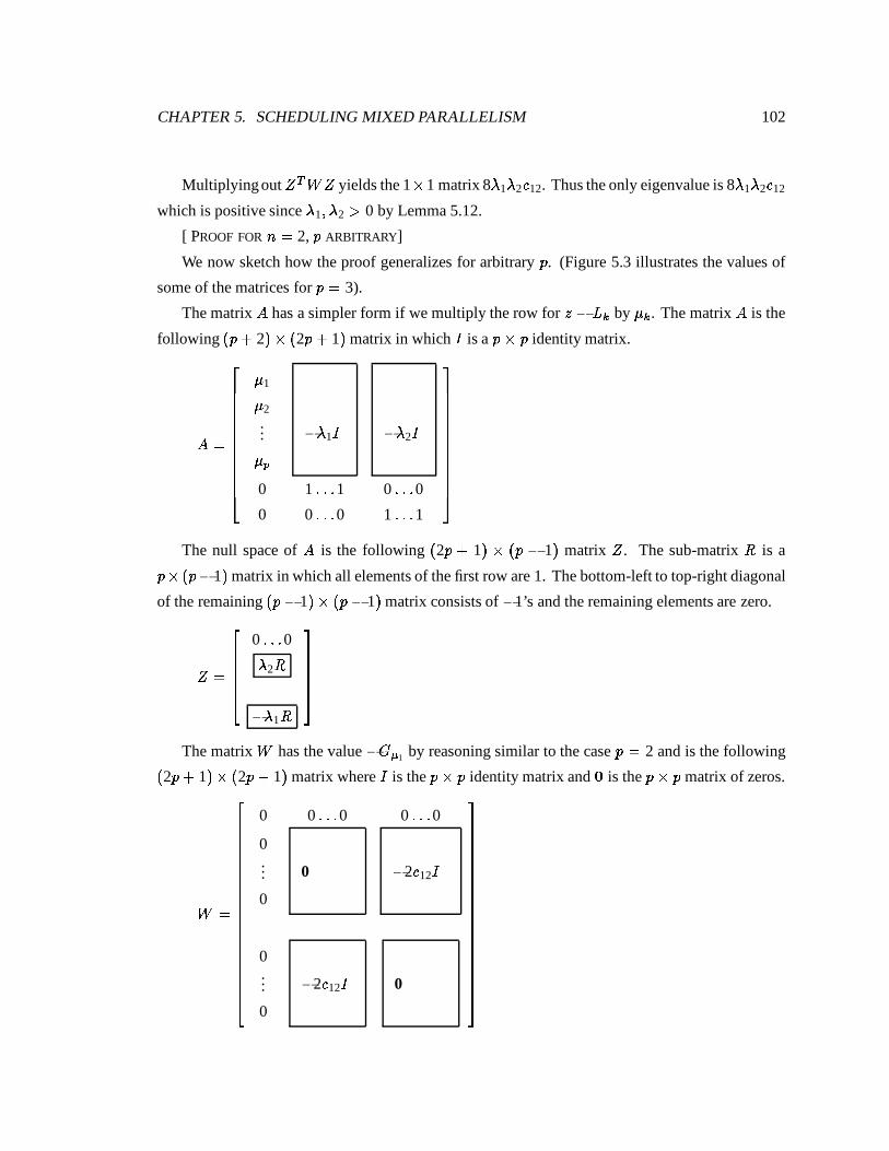
Transcript
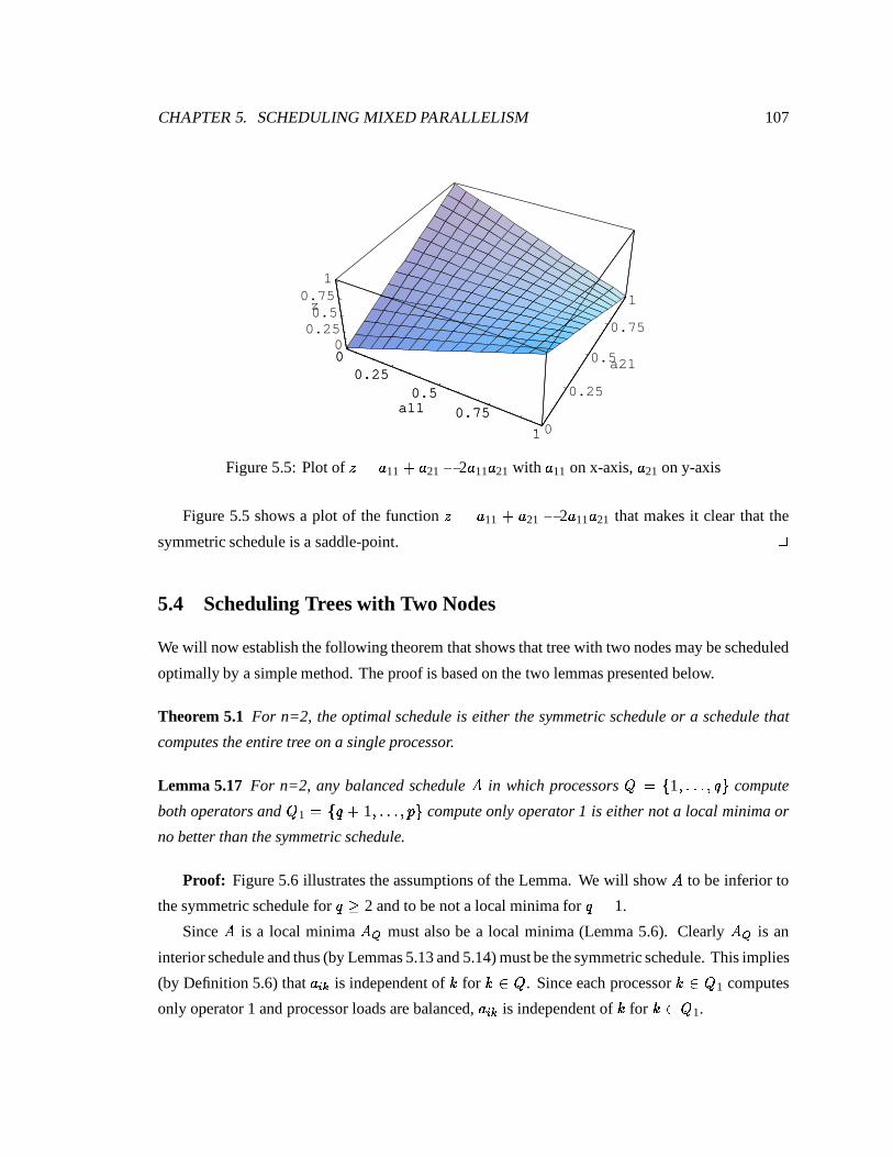
OPTIMIZATION OF SQL QUERIES FOR PARALLEL MACHINES
A DISSERTATION
SUBMITTED TO THE DEPARTMENT OF COMPUTER SCIENCE
AND THE COMMITTEE ON GRADUATE STUDIES
OF STANFORD UNIVERSITY
IN PARTIAL FULFILLMENT OF THE REQUIREMENTS
FOR THE DEGREE OF
DOCTOR OF PHILOSOPHY
By
Waqar Hasan
December, 1995
c Copyright 1996 by Waqar Hasan
All Rights Reserved
ii
I certify that I have read this dissertation and that in my opinion it is fully adequate,
in scope and in quality, as a dissertation for the degree of Doctor of Philosophy.
Gio Wiederhold(Principal Adviser)
I certify that I have read this dissertation and that in my opinion it is fully adequate,
in scope and in quality, as a dissertation for the degree of Doctor of Philosophy.
Hector Garcia-Molina
I certify that I have read this dissertation and that in my opinion it is fully adequate,
in scope and in quality, as a dissertation for the degree of Doctor of Philosophy.
Ravi Krishnamurthy
I certify that I have read this dissertation and that in my opinion it is fully adequate,
in scope and in quality, as a dissertation for the degree of Doctor of Philosophy.
Rajeev Motwani
I certify that I have read this dissertation and that in my opinion it is fully adequate,
in scope and in quality, as a dissertation for the degree of Doctor of Philosophy.
Jeffrey D. Ullman
Approved for the University Committee on Graduate Studies:
Dean of Graduate Studies
iii
Abstract
Parallel execution offers a solution to the problem of reducing the response time of SQL queries
against large databases. As a declarative language, SQL allows users to avoid the complex proce-
dural details of programming a parallel machine. A DBMS answers a SQL query by first finding
a procedural plan to execute the query and subsequently executing the plan to produce the query
result. We address the problem of parallel query optimization which is: Given a SQL query, find
the parallel plan that delivers the query result in minimal time.
We develop optimization algorithms using models that incorporate the sources of parallelism as
well as obstacles to achieving speedup. One obstacle is inherent limits on available parallelism due
to parallel and precedence constraints between operators and due to data placement constraints that
essentially pre-allocate some subset of operators. Another obstacle is that the overhead of exploiting
parallelism may increase total work thus reducing or even offsetting the benefit of parallel execution.
Our experiments with NonStop SQL, a commercial parallel DBMS, show communication of data
across processors to be a significant source of increase in work.
We adopt a two-phase approach to parallel query optimization: join ordering and query rewrite
(JOQR), followed by parallelization. The JOQR phase minimizes the total work to compute a query.
The parallelization phase extracts parallelism and schedules resources to minimize response time.
We make contributions to both phases. Our work is applicable to queries that include operations
such as grouping, aggregation, foreign functions, intersection and set difference in addition to joins.
We develop algorithms for the JOQR phase that minimize total cost while accounting for the
communication cost of repartitioning data. Using a model that abstracts physical characteristics
of data, such as partitioning, as colors, we devise tree coloring algorithms that are efficient and
guarantee optimality.
We model the parallelization phase as scheduling a tree of inter-dependent operators with
computation and communication costs represented as node and edge weights. Scheduling a weighted
operator tree on a parallel machine poses a class of novel multi-processor scheduling problems that
iv
differ from the classical in several ways.
We develop and compare several efficient algorithms for the problem of scheduling a pipelined
operator tree in which all operators run in parallel using inter-operator parallelism. Given the NP-
hardness of the problem, we assess the quality of our algorithms by measuring their performance
ratio which is the ratio of the response time of the generated schedule to that of the optimal. We
prove worst-case bounds on the performance ratios of our algorithms and measure the average cases
using simulation.
We address the problem of scheduling a pipelined operator tree using both pipelined and
partitioned parallelism. We characterize optimal schedules and investigate two classes of schedules
that we term symmetric and balanced.
The results in this thesis enable the construction of SQL compilers that can effectively exploit
parallel machines.
v
Acknowledgements
I express my gratitude to the people and organizations that made this thesis possible. Gio Wiederhold
was a constant source of intellectual support. He encouraged me to learn and use a variety
of techniques from different areas of Computer Science. Rajeev Motwani helped enhance my
understanding of theory and contributed significantly to the ideas in this thesis. Jeff Ullman was
a source of useful discussions and I thank him for his helpful and incisive comments. Ravi
Krishnamurthy served as a mentor and a source of interesting ideas and challenging questions.
Hector Garcia-Molina provided helpful advice. Jim Gray helped me understand the realities of
parallel query processing.
My thesis topic grew out of work at Hewlett-Packard Laboratories and was supported by a
fellowship from Hewlett-Packard. I express my gratefulness to Hewlett-Packard Company and
thank my managers Umesh Dayal, Dan Fishman, Peter Lyngbaek and Marie-Anne Neimat for
management, intellectual and moral support.
I thank Tandem Computers for providing access to a parallel machine, to the NonStop SQL/MP
parallel DBMS, and permitting publication of experimental results. I am grateful to Susanne Englert,
Ray Glasstone and Shyam Johari for making this possible and for helping me understand Tandem
systems.
The following friends and colleagues were a source of invaluable discussions and diversions:
Sang Cha, Surajit Chaudhuri, Philippe DeSmedt, Mike Heytens, Curt Kolovson, Stephanie Leichner,
Sheralyn Listgarten, Arif Merchant, Inderpal Mumick, Pandu Nayak, Peter Rathmann, Donovan
Schneider, Arun Swami, Kevin Wilkinson, Xiaolei Qian.
This thesis would not have been possible without the support and understanding of my family.
I thank my father, Dr. Amir Hasan, for providing the inspiration to pursue a PhD. I thank my
mother, Fatima Hasan, my brothers Safdar, Javed, and Zulfiquar, and sister Seemin for their love
and encouragement. I owe a debt to my wife Shirin and son Arif for putting up with my long hours
and for the support, love and encouragement that made this work possible.
Database systems provide competitive advantage to businesses by allowing quick determination of
answers to business questions. Intensifying competition continues to increase the sizes of databases
as well as the sophisticationof queries against them. Parallel machines constructed from commodity
hardware components offer higher performance as well as performance at a lower price as compared
to sequential mainframes. Exploiting parallelism is therefore a natural solution for reducing the
response times of queries against large databases.
SQL, the standard language for database access, is a declarative language. It insulates users from
the complex procedural details of accessing and manipulating data. In particular, exploiting parallel
machines does not require users to learn a new language or existing SQL code to be rewritten.
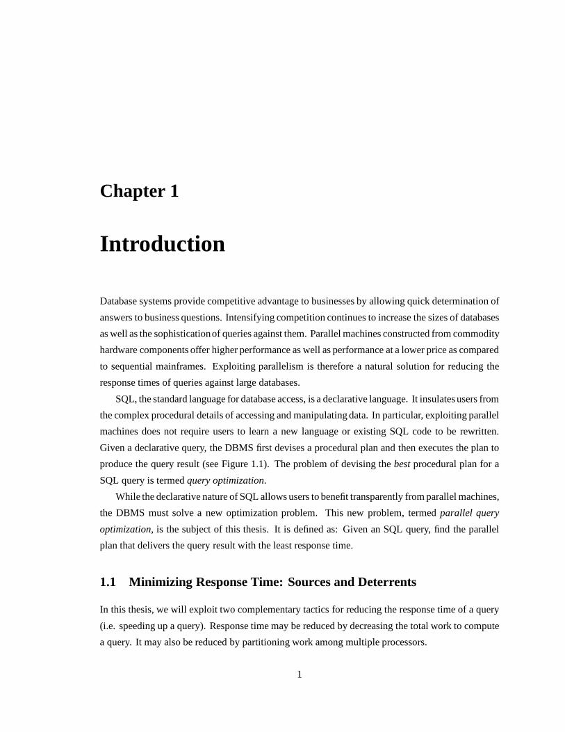
Given a declarative query, the DBMS first devises a procedural plan and then executes the plan to
produce the query result (see Figure 1.1). The problem of devising the best procedural plan for a
SQL query is termed query optimization.
While the declarative nature of SQL allows users to benefit transparently from parallel machines,
the DBMS must solve a new optimization problem. This new problem, termed parallel query
optimization, is the subject of this thesis. It is defined as: Given an SQL query, find the parallel
plan that delivers the query result with the least response time.
1.1 Minimizing Response Time: Sources and Deterrents
In this thesis, we will exploit two complementary tactics for reducing the response time of a query
(i.e. speeding up a query). Response time may be reduced by decreasing the total work to compute
a query. It may also be reduced by partitioning work among multiple processors.
1
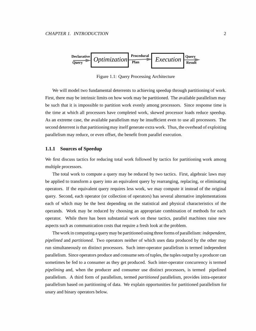
CHAPTER 1. INTRODUCTION 2
Declarative Procedural
PlanQuery
Query
ResultExecutionOptimization
Figure 1.1: Query Processing Architecture
We will model two fundamental deterrents to achieving speedup through partitioning of work.
First, there may be intrinsic limits on how work may be partitioned. The available parallelism may
be such that it is impossible to partition work evenly among processors. Since response time is
the time at which all processors have completed work, skewed processor loads reduce speedup.
As an extreme case, the available parallelism may be insufficient even to use all processors. The
second deterrent is that partitioning may itself generate extra work. Thus, the overhead of exploiting
parallelism may reduce, or even offset, the benefit from parallel execution.
1.1.1 Sources of Speedup
We first discuss tactics for reducing total work followed by tactics for partitioning work among
multiple processors.
The total work to compute a query may be reduced by two tactics. First, algebraic laws may
be applied to transform a query into an equivalent query by rearranging, replacing, or eliminating
operators. If the equivalent query requires less work, we may compute it instead of the original
query. Second, each operator (or collection of operators) has several alternative implementations
each of which may be the best depending on the statistical and physical characteristics of the
operands. Work may be reduced by choosing an appropriate combination of methods for each
operator. While there has been substantial work on these tactics, parallel machines raise new
aspects such as communication costs that require a fresh look at the problem.
The work in computing a query may be partitioned using three forms of parallelism: independent,
pipelined and partitioned. Two operators neither of which uses data produced by the other may
run simultaneously on distinct processors. Such inter-operator parallelism is termed independent
parallelism. Since operators produce and consume sets of tuples, the tuples output by a producer can
sometimes be fed to a consumer as they get produced. Such inter-operator concurrency is termed
pipelining and, when the producer and consumer use distinct processors, is termed pipelined
parallelism. A third form of parallelism, termed partitioned parallelism, provides intra-operator
parallelism based on partitioning of data. We explain opportunities for partitioned parallelism for
unary and binary operators below.
CHAPTER 1. INTRODUCTION 3
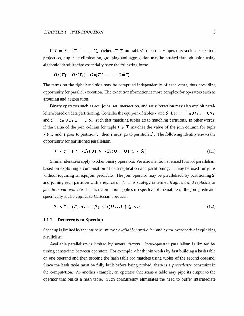
If T = T0 [ T1 [ : : : [ Tk (where T; Ti are tables), then unary operators such as selection,
projection, duplicate elimination, grouping and aggregation may be pushed through union using
algebraic identities that essentially have the following form:
Op(T ) = Op(T0) [Op(T1) [ : : :[ Op(Tk)
The terms on the right hand side may be computed independently of each other, thus providing
opportunity for parallel execution. The exact transformation is more complex for operators such as
grouping and aggregation.
Binary operators such as equijoins, set intersection, and set subtraction may also exploit paral-
lelism based on data partitioning. Consider the equijoin of tablesT andS. Let T = T0[T1[: : :[Tkand S = S0 [ S1 [ : : :[ Sk such that matching tuples go to matching partitions. In other words,
if the value of the join column for tuple t 2 T matches the value of the join column for tuple
s 2 S and, t goes to partition Ti then s must go to partition Si. The following identity shows the
opportunity for partitioned parallelism.
T ./ S = (T1 ./ S1) [ (T2 ./ S2) [ : : :[ (Tk ./ Sk) (1.1)
Similar identities apply to other binary operators. We also mention a related form of parallelism
based on exploiting a combination of data replication and partitioning. It may be used for joins
without requiring an equijoin predicate. The join operator may be parallelized by partitioning T
and joining each partition with a replica of S. This strategy is termed fragment and replicate or
partition and replicate. The transformation applies irrespective of the nature of the join predicate;
specifically it also applies to Cartesian products.
T ./ S = (T1 ./ S)[ (T2 ./ S)[ : : :[ (Tk ./ S) (1.2)
1.1.2 Deterrents to Speedup
Speedup is limited by the intrinsic limits on available parallelismand by the overheads of exploiting
parallelism.
Available parallelism is limited by several factors. Inter-operator parallelism is limited by
timing constraints between operators. For example, a hash join works by first building a hash table
on one operand and then probing the hash table for matches using tuples of the second operand.
Since the hash table must be fully built before being probed, there is a precedence constraint in
the computation. As another example, an operator that scans a table may pipe its output to the
operator that builds a hash table. Such concurrency eliminates the need to buffer intermediate
CHAPTER 1. INTRODUCTION 4
results. However, it places a parallel constraint in the computation. In many machine architectures,
data on a specific disk may be accessed only by the processor that controls the disk. Thus data
placement constraints limit both inter and intra-operator parallelism by localizing scan operations
to specific processors. For example, if an Employee table is stored partitioned by department, a
selection query that retrieves employees from a single department has no available parallelism.
Using parallel execution requires starting and initializing processes. These processes may then
communicate substantial amounts of data. These startup and communication overheads increase
total work. The increase is significant enough that careless use of parallelism can result in slowing
down queries rather than speeding them up. The cost of communication is a function of the size
of data communicated. While an individual operator may examine a relatively small portion of
each tuple, all attributes that are used by any subsequent operator need to be communicated. Thus,
communication costs can be an arbitrarily high portion of total cost.
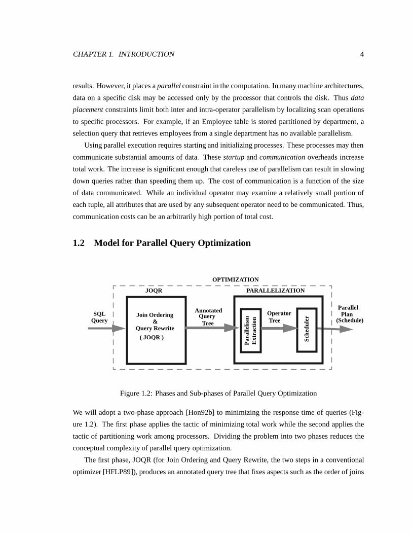
1.2 Model for Parallel Query Optimization
SQL
PARALLELIZATION
QueryParallel
Ext
ract
ion
Par
alle
lism
Sch
edul
erPlan
TreeQuery (Schedule)
OPTIMIZATION
( JOQR )
Annotated
TreeOperatorJoin Ordering
&Query Rewrite
JOQR
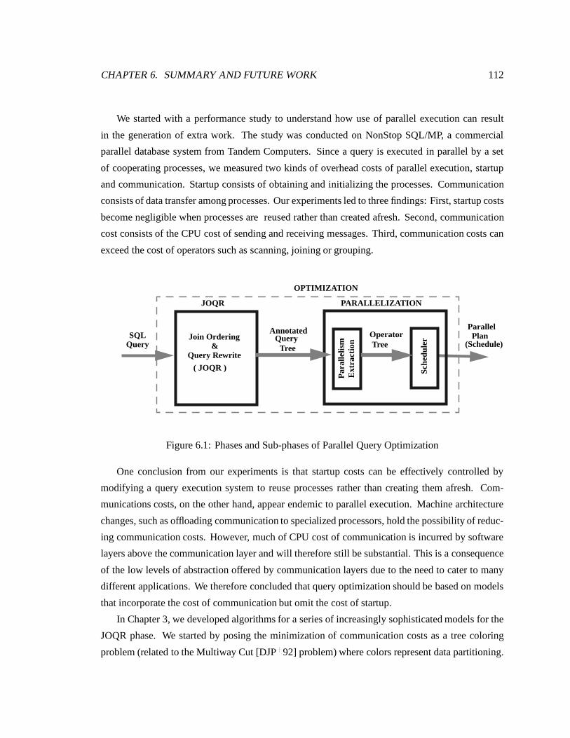
Figure 1.2: Phases and Sub-phases of Parallel Query Optimization
We will adopt a two-phase approach [Hon92b] to minimizing the response time of queries (Fig-
ure 1.2). The first phase applies the tactic of minimizing total work while the second applies the
tactic of partitioning work among processors. Dividing the problem into two phases reduces the
conceptual complexity of parallel query optimization.
The first phase, JOQR (for Join Ordering and Query Rewrite, the two steps in a conventional
optimizer [HFLP89]), produces an annotated query tree that fixes aspects such as the order of joins
CHAPTER 1. INTRODUCTION 5
and the strategy for computing each join. While conventional query optimization deals with similar
problems we will develop (in Chapter 3) models and algorithms that are cognizant of critical aspects
of parallel execution. Thus rather than finding the best plan for sequential execution, our algorithms
find the best plan while accounting for parallel execution.
The second phase, parallelization, converts the annotated query tree into a parallel plan. We
break the parallelization phase into two steps, parallelism extraction followed by scheduling.
Parallelism extraction produces an operator tree that identifies the atomic units of execution and
their interdependence. It explicates the timing constraints among operators. We shall briefly discuss
the extraction of parallelism in Section 1.2.2.
The scheduling step allocates machine resources to each operator. We shall develop models and
algorithms for several scheduling problems in Chapters 4 and 5.
1.2.1 Annotated Query Trees
A procedural plan for an SQL query is conventionally represented by an annotated query tree.
Such trees encode procedural choices such as the order in which operators are evaluated and the
method for computing each operator. Each tree node represents one (or several) relational operators.
Annotations on the node represent the details of how it is to be executed. For example a join node
may be annotated as being executed by a hash-join, and a base relation may be annotated as
being accessed by an index-scan. The EXPLAIN statement of most SQL systems (such as NonStop
SQL/MP [Tan94]) allows such trees to viewed by a user.
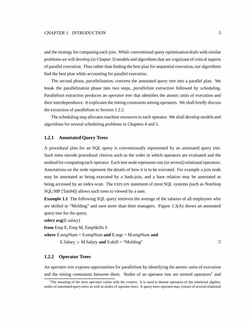
Example 1.1 The following SQL query retrieves the average of the salaries of all employees who
are skilled in “Molding” and earn more than their managers. Figure 1.3(A) shows an annotated
query tree for the query.
select avg(E.salary)
from Emp E, Emp M, EmpSkills S
where E.empNum = S.empNum and E.mgr = M.empNum and
E.Salary > M.Salary and S.skill = “Molding” 2
1.2.2 Operator Trees
An operator tree exposes opportunities for parallelism by identifying the atomic units of execution
and the timing constraints between them. Nodes of an operator tree are termed operators1 and1The meaning of the term operator varies with the context. It is used to denote operators of the relational algebra,
nodes of annotated query trees as well as nodes of operator trees. A query trees operator may consist of several relational
CHAPTER 1. INTRODUCTION 6
EMPSKILLS S
EMP M
EMP E
simple-hash
sort-merge
scan
index-scanclusteredindx-scan
AVG
Merge
Probe
IndexScan(S)
BuildClusteredScan(E)
Scan(M)
Avg
FormRuns
MergeRuns
S.empNum = E.empNum
E.mgr = M.empNum
(A) (B)
Figure 1.3: (A) Annotated Query Tree (B) Corresponding Operator Tree
represent pieces of code that are deemed to be atomic. Edges represent the flow of data as well as
timing constraints between these operators.
An operator takes zero or more input sets of tuples and produces a single output set. Operators
are formed by appropriate factoring of the code that implements the relational operations specified
in an annotated query tree. A criteria in designing operators is to reduce inter-operator timing
constraints to simple forms, i.e. parallel and precedence constraints.
The process of parallelism extraction is used to create operator trees from annotated query trees.
This process may be viewed as applying a “macro-expansion” to each node of an annotated query
tree. Since annotated query trees are constructed out of a fixed set of operators, the macro-expansion
of each operator (of an annotated query tree) may be specified using mechanism such as rules. We
will illustrate a sample expansion in Example 1.2.
Given an edge from operator i to j, a parallel constraint requires i and j to start at the same
time and terminate at the same time. A precedence constraint requires j to start after i terminates.
We define an edge that represents a parallel constraint to be a pipelining edge and an edge that
represents a precedence constraint to be a blocking edge.
Parallel constraints capture pipelined execution. A pipeline between two operators is typically
implemented using a flow control mechanism (such as a table queue [PMC+90]) to ensure that a
fixed amount of memory suffices for the pipeline. Flow-control causes a fast producer to be slowed
down by a slow consumer (or vice-versa) by stretching over a longer time period. Thus, the producer
and consumer operators are constrained to run concurrently. Precedence constraints capture the
operators. An operator tree operator is a piece of code that may not correspond to any relational or query tree operator.
CHAPTER 1. INTRODUCTION 7
behavior of operators that produce their output set only when they terminate. A consumer operator
must wait for the producer to terminate before it may start execution.
Example 1.2 Figure 1.3(B) shows the operator tree for the annotated query tree of Figure 1.3(A).
Thin edges are pipelining edges, thick edges are blocking. A simple hash join is broken into Build
and Probe operators. Since a hash table must be fully built before it can be probed, the edge
from Build to Probe is blocking. A sort-merge join sorts both inputs and then merges the sorted
streams. The merging is implemented by the Merge operator. In this example, we assume the
right input of sort-merge to be presorted. The operator tree shows the sort required for the left input
broken into two operators FormRuns and MergeRuns. Since the merging of runs can start only
after run formation, the edge from FormRuns to MergeRuns is blocking. 2
The operator tree exposes available parallelism. Partitioned parallelism may be used for any
operator. Pipelined parallelism may be used for operators connected by pipelining edges. Two
subtrees with no (transitive) precedence constraints between them may run independently. For ex-
ample, the subtrees rooted at FormRuns andBuildmay run independently; operators FormRuns
and Scan(M) may use pipelined parallelism; any operator may use partitioned parallelism.
1.2.3 Parallel Machine Model
We consider a parallel machine to consist of several identical nodes that communicate over an
interconnect. The cost of a message consists of CPU cost incurred equally by both the sending and
the receiving CPU. This cost is a function of the message size but independent of the identities of the
sending and receiving CPUs (as long as they are distinct). In other words, we consider propagation
delays and network topology to be irrelevant.
Propagation delay is the time delay for a single packet to travel over the interconnect. Query
processing results in communicating large amounts of data over the interconnect. Such communi-
cation is typically achieved by sending a stream of packets – packets continue to be sent without
waiting for already sent packets to reach the receiver. Thus, the propagation delay is independent
of the number of packets and becomes insignificant when the number of packets is large.
Network topology is ignored for three reasons. First, it is unclear whether the behavior of
sophisticated interconnects can be captured by simple topological models. Besides topological
properties, interconnects also have embedded memory and specialized processors. Second, most
architectures expect applications to regard the interconnect as a blackbox that has internal algorithms
for managing messages. Third, there is tremendous variation in the topologies used for interconnects.
CHAPTER 1. INTRODUCTION 8
Topology-dependent algorithms and software will be not be portable. Further, topology changes
even in a specific machine as nodes fail and recover or are added or removed. Correctly and reliably
adapting to such changes is complex. Incorporating topological knowledge in query processing and
optimization will further complicate these tasks.
1.3 Organization of Thesis
In Chapter 2, we start with an experimental study that compares parallel and sequential execution
in NonStop SQL/MP, a commercial parallel database system from Tandem Computers. The ex-
periments establish communication to be a significant overhead in using parallel execution. They
also show that startup costs may be made insignificant by modifying the execution system to reuse
processes rather than creating them afresh.
In Chapter 3, we deal with models and algorithms for the JOQR phase. We pose minimizing
communication as a tree coloring problem that is related to classical Multiway Cut problems. We
then enhance the model to cover aspects such as the dependence of operator costs on physical
properties of operands, the availability of multiple methods for an operator, and re-ordering of
operators. The chapter also provide a clean abstraction of the basic ideas in the commercially
popular System R algorithm.
In Chapter 3, we focuses on the parallelization phase and consider the problem of managing
pipelined parallelism. We start by developing the notion of worthless parallelism and showing
how such parallelism may be eliminated. We then develop a variety of scheduling algorithms that
assign operators to processors. We evaluate the algorithms by measuring their performance ratio
which is the response time of the produced schedule divided by the response time of the optimal
schedule. We establish bounds on the worst-case performance ratio by analytical methods and
measure average-case performance ratios by experiments.
In Chapter 5, we consider the problem of scheduling a pipelined tree using both pipelined and
partitioned parallelism. This is the continuous version of the discrete problem considered in the
last chapter. We develop characterizations of optimal schedules and investigate two classes of
schedules: symmetric and balanced.
Finally, in Chapter 6, we summarize our contributions and discuss some open problems.
CHAPTER 1. INTRODUCTION 9
1.4 Related Work
In this section, we discuss relevant past work in databases. The individual chapters will discuss
related work from theory (Multiprocessor Scheduling [Gra69, Ull75], Multiway Cuts [DJP+92]
and Nonlinear optimization [GMW81, Lue89]) that we will find useful in developing optimization
algorithms.
1.4.1 Query Optimization for Centralized Databases
Early work in query optimization followed two tracks. One was minimization of expression
size [CM77, ASU79]. Expression size was measured by metrics, such as the number of joins in a
query, that are independent of the database state. Another track was the development of heuristics
based on models that considered the cost of an operator to depend on the size of its operands as
well the data structures in which the operands were stored. For example, the cost of a join was
estimated using the sizes of operands as well as whether an index to access an operand was available.
Examples of such heuristics are performing selections and projections as early as possible [Hal76]
and the Wong-Youseffi algorithm [WY76] for decomposing queries.
The System R project at IBM viewed the problem of selecting access paths and ordering join
operators as an optimization problem with the objective of minimizing the total machine resource
to compute a query [SAC+79]. The estimation of machine resources was based on a cost model
in which the cost of an operation depended on the statistical properties of operands (such as the
minimum and maximum values in each column), the availability of indexes and the order in which
tuples could be accessed. It also developed a combination of techniques to search for a good query
plan. One of these techniques, the use of dynamic programming to speed up search, has been
adopted by most commercial optimizers. Another technique, avoiding Cartesian products, is now
recognized to produce bad plans for “star” queries (common in decision-support applications) in
which a single large table is joined to several small tables.
System R also incorporated algebraic transformations that were applied as heuristics while
parsing queries. The Starburst project recognized the growing importance of such heuristic trans-
formations [Day87, Kin81, Kim82, GW87] by considering Query Rewrite to be a phase of opti-
mization [PHH92].
The growing importance of decision-support has led to a rejuvenation of interest in discovering
new transformations and algorithms to exploit the transformations [YL95, CS94, GHQ95, LMS94].
CHAPTER 1. INTRODUCTION 10
1.4.2 Query Optimization for Distributed Databases
While distributed and parallel databases are fundamentally similar, research in distributed query
optimization was done in the early 1980s, a time at which communication over a network was
prohibitively expensive and computer equipment was not cheap enough to be thrown at parallel
processing.
The assumption of communication as the primary bottleneck led to the development of query
execution techniques, notably semijoins [BC81], to reduce communication. Techniques for ex-
ploiting parallelism were largely ignored. For example, Apers et al. [AHY83] discuss independent
parallelism but do not discuss either pipelined or partitioned parallelism. Thus, for historical rea-
sons, the notion of distributed execution differs from parallel execution. Since the space of possible
executions for a query is different, the optimization problems are different.
While Apers et al. considered minimizing response time as an optimization objective, most
work, such as in SDD-1 [BGW+81] and R* [LMH+85, ML86], focused on minimizing resource
consumption. SDD-1 assumed communication as the sole cost while R* considered local processing
costs as well.
Techniques for distributing data using horizontal and vertical partitioning schemes [Ull89,
CNW83, OV91] were developed for distributed data that also find a use in exploiting parallelism.
1.4.3 Query Optimization for Parallel Databases
Several research projects such as Bubba [BCC+90], Gamma [DGS+90], DBS3 [ZZBS93], and
Volcano [Gra90] devised techniques for placement of base tables and explored a variety of parallel
execution techniques. This has yielded a well understood notion of parallel execution.
Considerable research has also been done on measuring the parallelism available in different
classes of shapes for join trees. Schneider [Sch90] identified right-deep trees (with hash-joins as the
join method) as providing considerable parallelism. Chen et al. [CLYY92] investigated segmented
right-deep trees and Ziane et al. [ZZBS93] investigated Zig-Zag trees. Such research focuses on
evaluating a class of shapes rather than optimizing a single query. It may be used to subset the space
of executions over which optimization should be performed.
Hong and Stonebraker [HS91] proposed the two-phase approach to parallel query optimization.
They used a conventional query optimizer as the first phase. For parallelization, they considered
exploiting partitioned and independent parallelism but not pipelined parallelism. While they ig-
nored communication costs, we note that Hong [Hon92b] conjectured the XPRS approach to be
CHAPTER 1. INTRODUCTION 11
inapplicable to architectures such as shared-nothing that have significant communication costs.
Hong [Hon92a] develops a parallelization algorithm to maximize machine utilization under
restrictive assumptions. The parallel machine is assumed to consist of a single disk (RAID) and
multiple processors and each operator is assumed to have CPU and IO requirements. Assuming that
two operators, one CPU-bound and the other IO-bound to always be available for simultaneous
execution, the algorithm computes the degree of partitioned parallelism for each operator so as to
fully utilize the disk and all CPUs.
Many other efforts in parallel query optimization [SE93, LST91, SYT93, CLYY92, HLY93,
ZZBS93] develop heuristics assuming parallel execution to have no extra cost.
Chapter 2
Price of Parallelism
This chapter is a case study of NonStop SQL/MP, a commercial parallel DBMS from Tandem
Computers1. We report experimental measurements of the overheads in parallel execution as
compared to sequential execution2. We also document the use of parallel execution techniques in a
commercial system.
Our experiments investigate two overheads of using parallel execution: startup and communi-
cation. Startup is the overhead of obtaining and initializing the set of processes used to execute
the query. Communication is the overhead of communicating data among these processes while
executing the query. The findings from the experiments may be summarized as:
� Startup costs are negligible if processes can be reused rather than created afresh.
� Communication cost consists of the CPU cost of sending and receiving messages.
� Communication costs can exceed the cost of operators such as scanning, joining or grouping
These findings lead to the important conclusion that
Query optimization should be concerned with communication costs but not with startup costs.
1We thank Tandem Computers for providing access to NonStop SQL/MP and a parallel machine. Parts of this chapterhave also been published as the paper S. Englert, R. Glasstone and W. Hasan: Parallelism and its Price: A Case Studyof NonStop SQL/MP, Sigmod Record, Dec 1995
2We used the following guidelines to prevent commercial misuse of our experimental results: (a) All execution timesare scaled by a fixed but unspecified factor. (b) All query executions were created by bypassing the NonStop SQLoptimizer and no inference should be drawn about its behavior.
12
CHAPTER 2. PRICE OF PARALLELISM 13
2.1 Introduction
Startup overhead is incurred as a prelude to real work. It consists of obtaining a set of processes
and passing to each a description of its role in executing the query. The description consists of the
portion of the query plan the process will execute and the identities of the other processes it will
communicate with.
Communication overhead is the cost of transferring data between processes. Our experiments
consider three categories of communication between processes. Local communication consists of a
producer process sending data to a consumer process on the same processor. Remote communication
is the case when the producer and consumer are on distinct processors. Repartitioned communication
consists of a set of producers sending data to a set of consumers. Each tuple is routed based on the
value of some attribute.
Communication requires data to be moved from one physical location to another. Local
communication is implemented as a memory to memory copy across address spaces. Remote
communication divides data into packets that are transmitted across the interconnect. The receiving
CPU has to process interrupts generated by packet arrival as well as to reassemble the data. In
repartitioned communication, a producer has to perform some additional computation to determine
the destination of each tuple.
Our experiments compare the cost of communication with the cost of operators such as scans,
joins and groupings. We observe that while the cost of communicating data is proportional to the
number of bytes transmitted, an operator may not even look at all its input data – it only needs
to look at attributes that are relevant to it and may ignore the attributes that are relevant only to
subsequent operators.
We first describe the architecture of Tandem systems in Section 2.2. In Section 2.3, we
describe how opportunities for parallelism are exploited by NonStop SQL/MP. We then describe
our experimental results on startup costs in Section 2.4. Section 2.5 describes our results on the cost
of communication. These costs are put in perspective by comparing them with costs of operators
such as scans, joins and groupings. Section 2.6 shows interesting examples of parallel and sequential
execution and Section 2.7 summarizes our conclusions.
CHAPTER 2. PRICE OF PARALLELISM 14
Processor+ local
memoryProcessor
+ localmemory
Channel
Inter-Processor Bus
(A) (B)
Controller
Figure 2.1: (a) Tandem Architecture (b) Abstraction as Shared-Nothing
2.2 Tandem Architecture: An Overview
2.2.1 Parallel and Fault-tolerant Hardware
Tandem systems are fault-tolerant, parallel machines. For the purpose of query processing, a Tandem
system may be viewed as a classical shared-nothing system (see Figure 2.1). Each processor has
local memory and exclusive control over some subset of the disks.
Processors communicate over an interconnection network. Up to 16 processors may be con-
nected to an interprocessor bus to form a node. A variety of technologies and topologies are used
to interconnect multiple nodes.
For fault-tolerance, each logical disk consists of a mirrored pair of physical disks. Disk
controllers ensure that a write request is executed on both disks. A read request is directed to the
disk that can service it faster; for example if both disks are idle, the request is directed to the one
with its read head closer to the data.
We will not discuss further fault-tolerance features of the Tandem architecture since they are
largely orthogonal to query processing. The interested reader is referred to [BBT88] for details.
2.2.2 Message Based Software
Messages implement interprocess communication as well as disk IO. Access to a disk is encapsulated
by an associated set of disk processes that run on the processor that controls the disk. They implement
the basic facilities for reading, writing and locking disk-resident data. An IO request is made by
sending a message to a disk process. Data read by a read request is also sent back to the requester
as a message. Use of a set of disk processes allows several requests to be processed concurrently.
Disk processes are system processes and, for the purpose of query processing, may be regarded as
being permanently in operation.
A single file may be partitioned across multiple disks by ranges of key values. This allows tables
CHAPTER 2. PRICE OF PARALLELISM 15
and indexes to be horizontally partitioned using range partitioning. The file system is cognizant of
partitioned files and can route messages based on the key value of a requested record.
2.2.3 Performance Characteristics
The interconnect used for communication between processors is engineered to provide high band-
width and performance. Experiments [Tan] have shown the message throughput between two
processors to be limited by CPU speed rather than the speed of the interprocessor bus.
The programming interface for messages provides location transparency. However, the im-
plementation mechanisms for inter and intraprocessor messages are different. An intraprocessor
message is transmitted by a memory-to-memory copy. An interprocessor message is broken into
packets and sent over the interconnect. Packet arrival generates interrupts at the receiving CPU. The
packets are then assembled and written into the memory of the receiving process. Measurements
show an intraprocessor message to be significantly cheaper than an interprocessor message.
A mirrored disk consists of two physical disks with identical data layout. As remarked earlier, a
write request is executed on both physical disks while a read is directed to the disk that can process
it faster. A mirrored pair processes read requests faster than a single physical disk while writes run
at about the same speed.
2.3 Parallelism in NonStop SQL/MP
NonStop SQL/MP uses intra-operator parallelism for scans, selection, projection, joins and grouping
and aggregation. Intra-operation parallelism uses replication as well as partitioning. Interoperator
parallelism is not used. The system does not, for example, use pipelined parallelism, in which
disjoint sets of processors are used for the producer and consumer. It does, however, use pipelined
execution whenever possible, in which producers and consumers run concurrently.
In Section 2.3.1, we discuss the use of intra-operator parallelism. Section 2.3.2 discusses how
operators are mapped to a processes and processes to processors.
2.3.1 Use of Intra-operator Parallelism
Intra-operator parallelism is based on data partitioning and replication. Recall that base tables and
indexes may be stored horizontally partitioned over several disks based on key ranges. Scans and
groupings are parallelized using the existing data partitioning.
CHAPTER 2. PRICE OF PARALLELISM 16
Joins may repartition or replicate data in addition to using the existing data partitioning. Such
repartitioning or replication occurs on the fly while processing a query and does not affect any stored
data. Data repartitioning is based on hashing and equally distributes data across all CPUs.
Stored data is scanned by disk processes that implement selection, projection and some kinds
of groupings and aggregation. Since each disk has its exclusive disk processes, the architecture
naturally supports parallel scans.
Grouping is implemented in two ways, one based on sorting and the other on hashing. Sort
grouping first sorts the data on the grouping columns and then computes the grouped aggregates by
traversing the tuples in order. Hash grouping forms groups by building a hash table based on the
grouping columns and then computes aggregates for each group.
The strategy for parallelizing a grouping is to use the existing data partitioning. A separate
grouping is done for each partition followed by a combination of the results. Data is not repartitioned
to change the degree of parallelism or the partitioning attribute.
A join of two tables (say T and S) may be parallelized in the following two ways corresponding
to Equations 1.2 and 1.1.
Partition Both: Both tables may be partitioned only when an equijoin predicate is available. If
both tables are similarly partitioned on the join column, the “matching” partitions may be joined.
Otherwise, one or both tables may be repartitioned.
Partition and Replicate: Another parallelization strategy is to partitionS and join each partition
of S with all of table T . This may be achieved in two ways. The first is to replicate T on all nodes
that contain a partition of S. The second is to repartition S (for example, to increase degree of
parallelism) and replicate T on all nodes with a (new) partition of S.
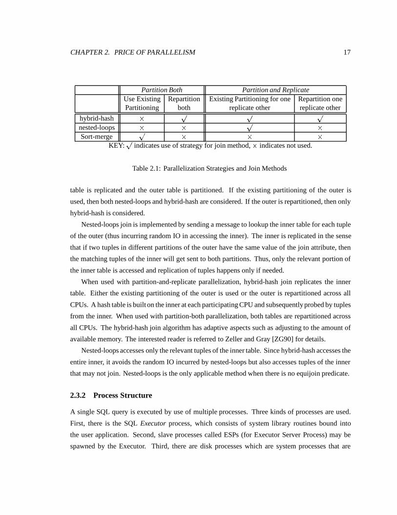
Three methods are used for joins: nested-loops, sort-merge and hybrid-hash. Table 2.1 summa-
rizes the join methods used for each parallelization strategy.
When both tables happen to be partitioned similarly by the join column, sort-merge join is the
most efficient join method. Since the partitioning columns are always identical to the sequencing
columns in NonStop SQL, the sorting step of sort-merge is skipped and the matching partitions are
simply merged.
In the strategy of repartitioning both tables, both are distributed across all CPUs using a hash
function on the joining columns. In this way, corresponding data from both tables or composites
is located such that it can be joined locally in each CPU using the hybrid hash-join method. The
strategy of repartitioning only one of the tables is not considered.
The partition-and-replicate strategy considers both nested-loops and hybrid-hash. The inner
CHAPTER 2. PRICE OF PARALLELISM 17
Partition Both Partition and ReplicateUse Existing Repartition Existing Partitioning for one Repartition onePartitioning both replicate other replicate other
hybrid-hash � p p pnested-loops � � p �Sort-merge
p � � �KEY:
pindicates use of strategy for join method, � indicates not used.
Table 2.1: Parallelization Strategies and Join Methods
table is replicated and the outer table is partitioned. If the existing partitioning of the outer is
used, then both nested-loops and hybrid-hash are considered. If the outer is repartitioned, then only
hybrid-hash is considered.
Nested-loops join is implemented by sending a message to lookup the inner table for each tuple
of the outer (thus incurring random IO in accessing the inner). The inner is replicated in the sense
that if two tuples in different partitions of the outer have the same value of the join attribute, then
the matching tuples of the inner will get sent to both partitions. Thus, only the relevant portion of
the inner table is accessed and replication of tuples happens only if needed.
When used with partition-and-replicate parallelization, hybrid-hash join replicates the inner
table. Either the existing partitioning of the outer is used or the outer is repartitioned across all
CPUs. A hash table is built on the inner at each participating CPU and subsequently probed by tuples
from the inner. When used with partition-both parallelization, both tables are repartitioned across
all CPUs. The hybrid-hash join algorithm has adaptive aspects such as adjusting to the amount of
available memory. The interested reader is referred to Zeller and Gray [ZG90] for details.
Nested-loops accesses only the relevant tuples of the inner table. Since hybrid-hash accesses the
entire inner, it avoids the random IO incurred by nested-loops but also accesses tuples of the inner
that may not join. Nested-loops is the only applicable method when there is no equijoin predicate.
2.3.2 Process Structure
A single SQL query is executed by use of multiple processes. Three kinds of processes are used.
First, there is the SQL Executor process, which consists of system library routines bound into
the user application. Second, slave processes called ESPs (for Executor Server Process) may be
spawned by the Executor. Third, there are disk processes which are system processes that are
CHAPTER 2. PRICE OF PARALLELISM 18
permanently in operation.
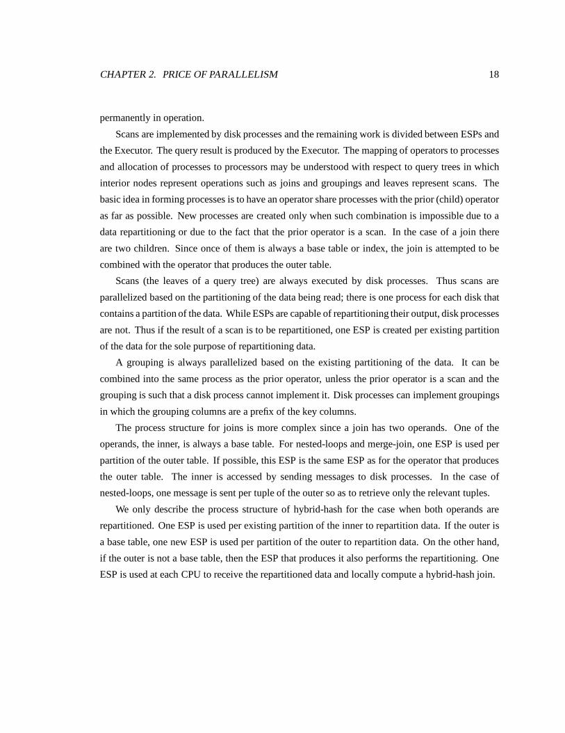
Scans are implemented by disk processes and the remaining work is divided between ESPs and
the Executor. The query result is produced by the Executor. The mapping of operators to processes
and allocation of processes to processors may be understood with respect to query trees in which
interior nodes represent operations such as joins and groupings and leaves represent scans. The
basic idea in forming processes is to have an operator share processes with the prior (child) operator
as far as possible. New processes are created only when such combination is impossible due to a
data repartitioning or due to the fact that the prior operator is a scan. In the case of a join there
are two children. Since once of them is always a base table or index, the join is attempted to be
combined with the operator that produces the outer table.
Scans (the leaves of a query tree) are always executed by disk processes. Thus scans are
parallelized based on the partitioning of the data being read; there is one process for each disk that
contains a partition of the data. While ESPs are capable of repartitioning their output, disk processes
are not. Thus if the result of a scan is to be repartitioned, one ESP is created per existing partition
of the data for the sole purpose of repartitioning data.
A grouping is always parallelized based on the existing partitioning of the data. It can be
combined into the same process as the prior operator, unless the prior operator is a scan and the
grouping is such that a disk process cannot implement it. Disk processes can implement groupings
in which the grouping columns are a prefix of the key columns.
The process structure for joins is more complex since a join has two operands. One of the
operands, the inner, is always a base table. For nested-loops and merge-join, one ESP is used per
partition of the outer table. If possible, this ESP is the same ESP as for the operator that produces
the outer table. The inner is accessed by sending messages to disk processes. In the case of
nested-loops, one message is sent per tuple of the outer so as to retrieve only the relevant tuples.
We only describe the process structure of hybrid-hash for the case when both operands are
repartitioned. One ESP is used per existing partition of the inner to repartition data. If the outer is
a base table, one new ESP is used per partition of the outer to repartition data. On the other hand,
if the outer is not a base table, then the ESP that produces it also performs the repartitioning. One
ESP is used at each CPU to receive the repartitioned data and locally compute a hybrid-hash join.
CHAPTER 2. PRICE OF PARALLELISM 19
2.4 Startup Costs
Parallel execution requires starting up a set of processes and communicating data among them. This
section measures startup cost and the next section focuses on communication.
When a query is executed in parallel, the Executor process starts up all necessary ESP processes
and sends to each the portion of the plan it needs to execute and the identities of the other processes
it needs to communicate with. The ESP processes are created sequentially; each process is created
and given its plan before the next process is created. ESPs are not terminated for 5 minutes after the
query completes. In case another query is executed within five minutes, ESP processes are reused.
We measured the cost of starting up processes by running a query that required 44 ESP processes.
Figure 2.2 plots the time at which successive processes got started and had received their portion
of the plan. The dotted line plots process startup when new processes had to be created. The solid
line plots the case when processes were reused.
We conclude that communicating the relevant portion of the plan to each ESP has negligible
cost. Startup cost is negligible when processes can be reused. Startup incurs an overhead of 0.5 sec
per process that needs to be created. A possible enhancement would be to start the ESP processes
in parallel instead of sequentially.
10 20 30 40Process#0
2.5
5
7.5
10
12.5
15
17.5
20
Elapsed Time (seconds)
Figure 2.2: Process Startup: With (solid) and without (dotted) process reuse.
2.5 Costs of Operators and Communication
In this section we measure the cost of communication and put these costs in perspective by a
comparison with operators such as scans, joins and grouping.
We describe measurements of the cost of local, remote and repartitioned communication. Local
CHAPTER 2. PRICE OF PARALLELISM 20
Local Remote Repartitioned
Figure 2.3: Local, Remote and Repartitioned Communication
communication consists of a producer process sending data to a consumer process on the same
processor. Remote communication is the case when the producer and consumer are on distinct
processors. In repartitioned communication, a set of producers send data to a set of producers. The
cost of repartitioning varies with the pattern of communication used. We decided to focus on the
case where a single producer partitions its output equally among a set of consumers. This simple
pattern captures the overhead of a producer sending data to multiple consumers i.e. the additional
overhead of determining the the destination of each tuple. The producer applies a hash function
to an attribute value to determine the CPU to which the tuple is to be sent. Figure 2.3 illustrates
the forms of communication covered by our experiments. These cases were chosen due to their
simplicity. The costs of other communication patterns may be extrapolated.
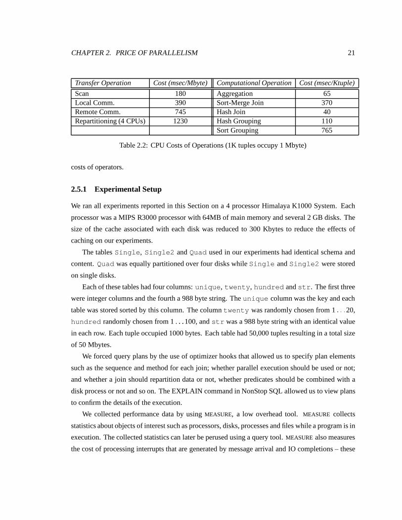
Table 2.2 summarizes the results of measurements that are described later in this section. It
turned out that the cpu time of all our queries was linear in the amount of data accessed. Even
operations that involved sorting behaved linearly in the range covered by our experiments. Thus
costs are stated in units of msec/Ktuple and msec/Mbyte. The two units are comparable, since 1K
tuples occupy 1 Mbyte for the table under consideration. Join costs were measured by joining two
tables, each with k tuples, to produce k output tuples. Join costs were linear in k and are therefore
reported in msec/Ktuple.
Our approach was to devise experiments such that the cost of an operation could be determined
as the difference of two executions. For instance the cost of local communication was determined
as the difference of executing the same query using two plans that only differed in whether one or
two processes were used.
Section 2.5.1 provides an overview of our experimental setup. Sections 2.5.3 and 2.5.4 describe
experiments that measure the cost of communication and Sections 2.5.2, 2.5.5 and 2.5.6 address the
CHAPTER 2. PRICE OF PARALLELISM 21
Transfer Operation Cost (msec/Mbyte) Computational Operation Cost (msec/Ktuple)
Table 2.2: CPU Costs of Operations (1K tuples occupy 1 Mbyte)
costs of operators.
2.5.1 Experimental Setup
We ran all experiments reported in this Section on a 4 processor Himalaya K1000 System. Each
processor was a MIPS R3000 processor with 64MB of main memory and several 2 GB disks. The
size of the cache associated with each disk was reduced to 300 Kbytes to reduce the effects of
caching on our experiments.
The tables Single, Single2 and Quad used in our experiments had identical schema and
content. Quad was equally partitioned over four disks while Single and Single2 were stored
on single disks.
Each of these tables had four columns: unique, twenty, hundred and str. The first three
were integer columns and the fourth a 988 byte string. The unique column was the key and each
table was stored sorted by this column. The column twenty was randomly chosen from 1 : : :20,
hundred randomly chosen from 1 : : :100, and str was a 988 byte string with an identical value
in each row. Each tuple occupied 1000 bytes. Each table had 50,000 tuples resulting in a total size
of 50 Mbytes.
We forced query plans by the use of optimizer hooks that allowed us to specify plan elements
such as the sequence and method for each join; whether parallel execution should be used or not;
and whether a join should repartition data or not, whether predicates should be combined with a
disk process or not and so on. The EXPLAIN command in NonStop SQL allowed us to view plans
to confirm the details of the execution.
We collected performance data by using MEASURE, a low overhead tool. MEASURE collects
statistics about objects of interest such as processors, disks, processes and files while a program is in
execution. The collected statistics can later be perused using a query tool. MEASURE also measures
the cost of processing interrupts that are generated by message arrival and IO completions – these
CHAPTER 2. PRICE OF PARALLELISM 22
costs are not assigned to any process.
Each data point reported in this paper is an average over three executions. Typically, the three
executions differed by less than 1%. All plotted curves were obtained using a least squares fit using
the Fit function in Mathematica.
2.5.2 Costs of Scans, Predicates and Aggregation
We used the following query to scan Single.
Query1: select unique from Single
where twenty > 50000 and unique < k
The predicatetwenty >50000 is false for all tuples. Thus no tuples are returned and the overhead
of communicating the result of the scan is eliminated. Since the table was stored sorted by unique,
the predicate unique < k allowed us to vary the portion of the table scanned.
The query plan used a single disk process and combined predicate evaluation with the scan. The
cost of the plan consists of a scan and two predicate evaluations, one of which is a key predicate.
The dotted line in Figure 2.4 plots the cost as k was varied from 5000 to 50000 in increments of
5000. Denoting cpu cost by t and the number of Mbytes scanned by b, a least squares fit yields the
equation t = 0:31 + 0:185b. Thus a scan with two predicates costs 185 msec/Mbyte.
We determined the cost of predicate checking by additional measurements. To measure the cost
of the key predicate, we tried two queries: one with the predicate unique < 100,000 and the
other with no key predicate. Both queries scanned the entire table, since all key values were less
than 100,000, and ran in identical time.
To measure the cost of the nonkey predicate, we ran a query with two nonkey predicates. The
“where clause” of Query1 was changed to (twenty >50000 or hundred >50000) and
unique1 < k. The solid lines in Figure 2.4 plots the cost of a query. Curve fitting yields
t = 0:31 + 0:18b i.e. the cost increases by 5 msec/Mbyte due to the additional nonkey predicate.
Thus, we may expect a scan with no predicates to cost 180 msec/Mbyte.
The dashed line in Figure 2.4 shows the cost of applying an aggregation in the disk process
using the following query.
Query2: select max(str) from Single
where unique < k
CHAPTER 2. PRICE OF PARALLELISM 23
10 20 30 40 50Mbytes0
2
4
6
8
10
12
14
CPU Time (seconds)
Figure 2.4: Scan with 1 predicate(dotted), 2 predicates(solid), aggregation(dashed)
A least square fit yielded the equation t = 0:31+0:245b. Subtracting scan cost, we infer aggregation
to cost (245-180) msec/Mbyte which is 65 msec/Mbyte. Recall that str is a 988 byte string with
an identical value in each row. Thus the aggregation uses 988 bytes of each 1000 byte tuple.
10 20 30 40 50Mbytes0
2
4
6
8
10
12
14
CPU Time (seconds)
(a)
(b), (c)
10 20 30 40 50Mbytes0
10
20
30
40
50
CPU Time (seconds)
(a)
(b)
(c)
(A) 98.8% of scanned data communicated (B) 4% of scanned data communicated
Figure 2.5: Scan and Aggregation(dashed) with Local(solid) and Remote(dotted) Comm.
2.5.3 Costs of Local and Remote Communication
We measured the cost of local and remote communication by use of optimizer hooks that permitted
the creation of plans in which the aggregation in Query2 was moved to a separate process (the
Executor) and the process could either be placed on the same CPU as the disk process or on a
different CPU. Figure 2.6 shows the process structure for the three executions.
CHAPTER 2. PRICE OF PARALLELISM 24
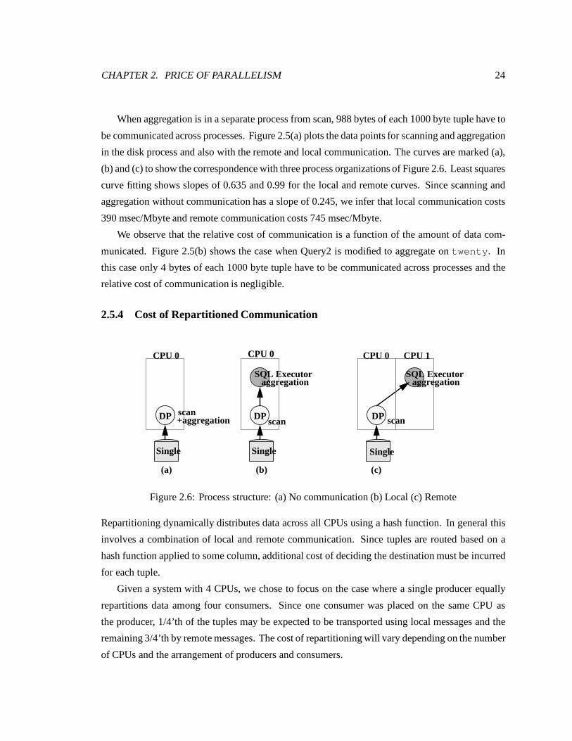
When aggregation is in a separate process from scan, 988 bytes of each 1000 byte tuple have to
be communicated across processes. Figure 2.5(a) plots the data points for scanning and aggregation
in the disk process and also with the remote and local communication. The curves are marked (a),
(b) and (c) to show the correspondence with three process organizations of Figure 2.6. Least squares
curve fitting shows slopes of 0.635 and 0.99 for the local and remote curves. Since scanning and
aggregation without communication has a slope of 0.245, we infer that local communication costs
390 msec/Mbyte and remote communication costs 745 msec/Mbyte.
We observe that the relative cost of communication is a function of the amount of data com-
municated. Figure 2.5(b) shows the case when Query2 is modified to aggregate on twenty. In
this case only 4 bytes of each 1000 byte tuple have to be communicated across processes and the
relative cost of communication is negligible.
2.5.4 Cost of Repartitioned Communication
DP DPscanscan
SQL Executor
DPscan
SQL Executor
+aggregation
aggregationaggregation
(a) (b) (c)
CPU 0 CPU 0 CPU 0 CPU 1
Single Single Single
Figure 2.6: Process structure: (a) No communication (b) Local (c) Remote
Repartitioning dynamically distributes data across all CPUs using a hash function. In general this
involves a combination of local and remote communication. Since tuples are routed based on a
hash function applied to some column, additional cost of deciding the destination must be incurred
for each tuple.
Given a system with 4 CPUs, we chose to focus on the case where a single producer equally
repartitions data among four consumers. Since one consumer was placed on the same CPU as
the producer, 1/4’th of the tuples may be expected to be transported using local messages and the
remaining 3/4’th by remote messages. The cost of repartitioning will vary depending on the number
of CPUs and the arrangement of producers and consumers.
CHAPTER 2. PRICE OF PARALLELISM 25
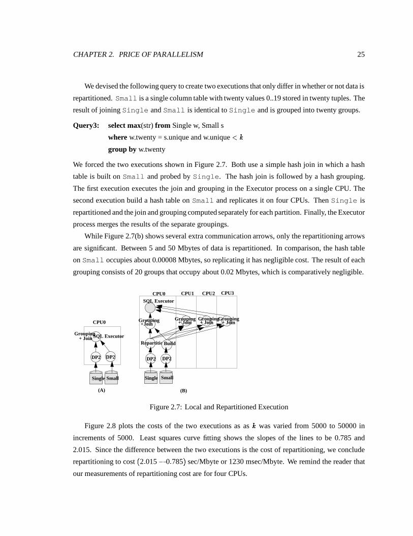
We devised the following query to create two executions that only differ in whether or not data is
repartitioned. Small is a single column table with twenty values 0..19 stored in twenty tuples. The
result of joining Single and Small is identical to Single and is grouped into twenty groups.
Query3: select max(str) from Single w, Small s
where w.twenty = s.unique and w.unique < k
group by w.twenty
We forced the two executions shown in Figure 2.7. Both use a simple hash join in which a hash
table is built on Small and probed by Single. The hash join is followed by a hash grouping.
The first execution executes the join and grouping in the Executor process on a single CPU. The
second execution build a hash table on Small and replicates it on four CPUs. Then Single is
repartitioned and the join and grouping computed separately for each partition. Finally, the Executor
process merges the results of the separate groupings.
While Figure 2.7(b) shows several extra communication arrows, only the repartitioning arrows
are significant. Between 5 and 50 Mbytes of data is repartitioned. In comparison, the hash table
on Small occupies about 0.00008 Mbytes, so replicating it has negligible cost. The result of each
grouping consists of 20 groups that occupy about 0.02 Mbytes, which is comparatively negligible.
DP2 DP2
SQL ExecutorRepartition
+ JoinGrouping
+ JoinGrouping
+ JoinGrouping
+ JoinGrouping
+JoinGrouping
(A) (B)
DP2 DP2
Build
Single Single Small
CPU0 CPU1 CPU2 CPU3
CPU0
Small
SQL Executor
Figure 2.7: Local and Repartitioned Execution
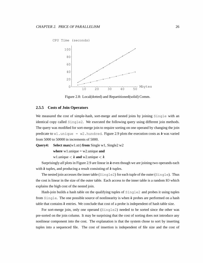
Figure 2.8 plots the costs of the two executions as as k was varied from 5000 to 50000 in
increments of 5000. Least squares curve fitting shows the slopes of the lines to be 0.785 and
2.015. Since the difference between the two executions is the cost of repartitioning, we conclude
repartitioning to cost (2:015� 0:785) sec/Mbyte or 1230 msec/Mbyte. We remind the reader that
our measurements of repartitioning cost are for four CPUs.
CHAPTER 2. PRICE OF PARALLELISM 26
10 20 30 40 50Mbytes0
20
40
60
80
100
CPU Time (seconds)
Figure 2.8: Local(dotted) and Repartitioned(solid) Comm.
2.5.5 Costs of Join Operators
We measured the cost of simple-hash, sort-merge and nested joins by joining Single with an
identical copy called Single2. We executed the following query using different join methods.
The query was modified for sort-merge join to require sorting on one operand by changing the join
predicate to w1.unique = w2.hundred. Figure 2.9 plots the execution costs as k was varied
from 5000 to 50000 in increments of 5000.
Query4: Select max(w1.str) from Single w1, Single2 w2
where w1.unique = w2.unique and
w1.unique < k and w2.unique < k
Surprisingly all plots in Figure 2.9 are linear in k even though we are joining two operands each
with k tuples, and producing a result consisting of k tuples.
The nested join accesses the inner table (Single2) for each tuple of the outer (Single). Thus
the cost is linear in the size of the outer table. Each access to the inner table is a random IO which
explains the high cost of the nested join.
Hash-join builds a hash table on the qualifying tuples of Single2 and probes it using tuples
from Single. The one possible source of nonlinearity is when k probes are performed on a hash
table that contains k entries. We conclude that cost of a probe is independent of hash table size.
For sort-merge join, only one operand (Single2) needed to be sorted since the other was
pre-sorted on the join column. It may be surprising that the cost of sorting does not introduce any
nonlinear component into the cost. The explanation is that the system chose to sort by inserting
tuples into a sequenced file. The cost of insertion is independent of file size and the cost of
CHAPTER 2. PRICE OF PARALLELISM 27
10 20 30 40 50k0
20
40
60
80
100
CPU Time (seconds)
Figure 2.9: Query using Simple-hash (dashed), Sort-merge (solid) and Nested Join (dotted)
comparisons is not a significant cost in locating the correct page.
Least squares curve fitting shows cost of the query to be 1835, 855 and 1185 msec/Mbyte for
nested, hash and sort-merge join respectively. The “per Mbyte” should be interpreted as “per Mbyte
of each operand”.
We may separate the cost of joining from the cost of scans, communication, and aggregation by
using our prior measurements.
For hash-join, we incur a scan for each operand. However, local communication is significant
only for Single. After projection, Single2 is reduced to 4/1000’th of its original size while
almost all (992/1000’th) of Single is communicated. Thus the cost of the join may be calculated
by subtracting the cost of two scans, the cost of locally communicating Single, and the cost of
aggregation. This gives us 855� (2 � 180 + 390 + 65) = 105 msec/Mbyte.
Similarly, the cost of a sort-merge join may be calculated to be 370 msec/Mbyte. The cost of
a nested-loops join cannot be broken down in this manner since it incurs a random IO per tuple of
Single.
2.5.6 Costs of Grouping Operators
NonStop SQL uses two algorithms for grouping. Hash grouping forms groups by hashing tuples
into a hash table based on the value of the grouping column. Sort grouping forms groups by sorting
the table on the grouping column. The following query reads k records and forms twenty groups.
Query5: select max(str) from Single
where unique < k
CHAPTER 2. PRICE OF PARALLELISM 28
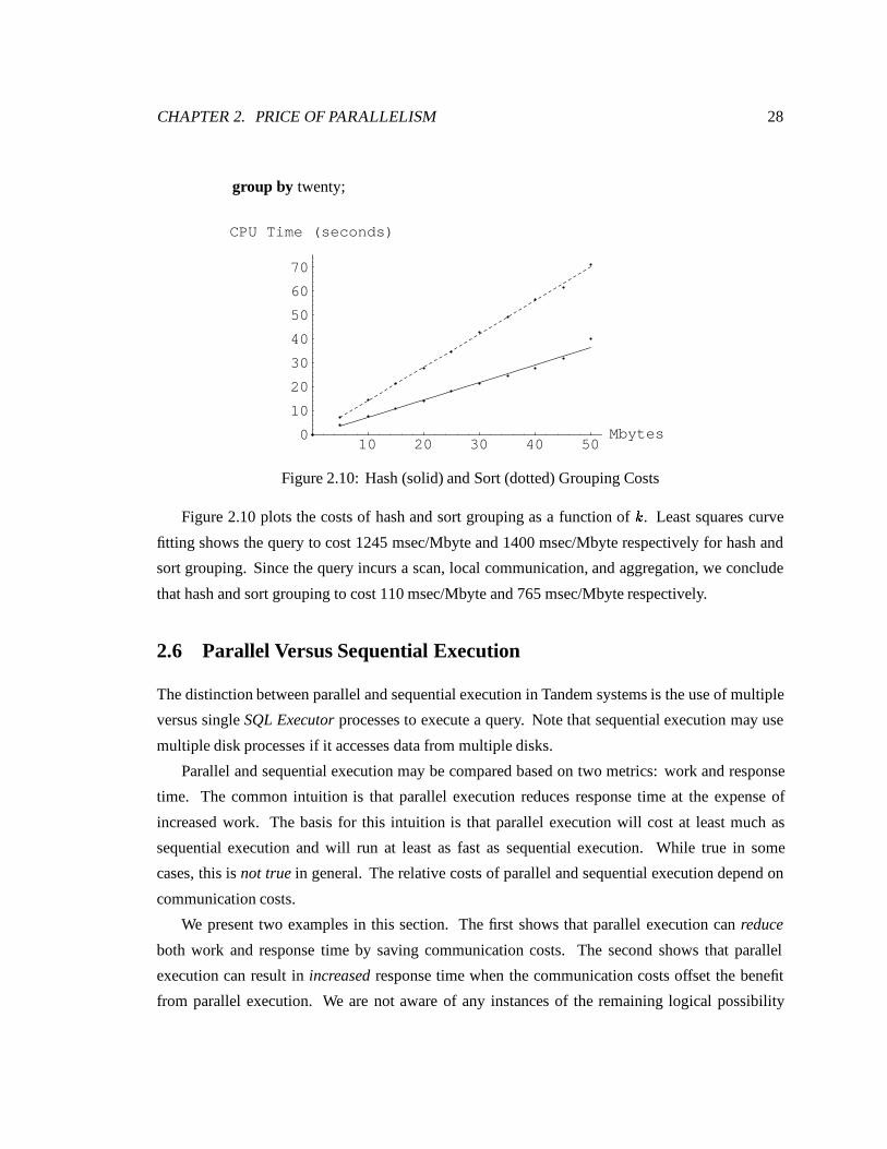
group by twenty;
10 20 30 40 50Mbytes0
10
20
30
40
50
60
70
CPU Time (seconds)
Figure 2.10: Hash (solid) and Sort (dotted) Grouping Costs
Figure 2.10 plots the costs of hash and sort grouping as a function of k. Least squares curve
fitting shows the query to cost 1245 msec/Mbyte and 1400 msec/Mbyte respectively for hash and
sort grouping. Since the query incurs a scan, local communication, and aggregation, we conclude
that hash and sort grouping to cost 110 msec/Mbyte and 765 msec/Mbyte respectively.
2.6 Parallel Versus Sequential Execution
The distinction between parallel and sequential execution in Tandem systems is the use of multiple
versus single SQL Executor processes to execute a query. Note that sequential execution may use
multiple disk processes if it accesses data from multiple disks.
Parallel and sequential execution may be compared based on two metrics: work and response
time. The common intuition is that parallel execution reduces response time at the expense of
increased work. The basis for this intuition is that parallel execution will cost at least much as
sequential execution and will run at least as fast as sequential execution. While true in some
cases, this is not true in general. The relative costs of parallel and sequential execution depend on
communication costs.
We present two examples in this section. The first shows that parallel execution can reduce
both work and response time by saving communication costs. The second shows that parallel
execution can result in increased response time when the communication costs offset the benefit
from parallel execution. We are not aware of any instances of the remaining logical possibility
CHAPTER 2. PRICE OF PARALLELISM 29
of parallel execution offering reduced work but increased response time compared to sequential
execution.
To sum up, in addition to the intuitive case in which parallel execution runs faster but consumes
more resources, it is possible that (a) parallel execution consumes less resources as well as runs faster
and (b) parallel execution consumes more resources as well as runs slower. The main determinant
is the cost of communication.
2.6.1 Parallelism can Reduce Work
The following query performs a grouping on a table that is equally partitioned across 4 disks, each
attached to a distinct CPU.
Query6: select max(str)
from Quad
group by twenty;
DP2
SQL Executor
SQL Executor
ESPs
(A) (B)
DP2 DP2 DP2
CPU 0 CPU 1 CPU 2 CPU 3
CPU 0 CPU 1 CPU 2 CPU 3
Quad
ESP ESP ESPGrouping
ESP }
DP2 DP2 DP2 DP2
Quad QuadQuadQuadQuadQuad Quad
Figure 2.11: Process Structure: Sequential and Parallel Execution
Figure 2.11 shows the process structure for sequential and parallel execution. When sequential
execution is used, SQL runs as a single process (Executor). This process must incur remote
communication to read the three partitions that reside on remote disks. When parallel execution is
used, the grouping is partitioned. Each partition of Quad is grouped separately by an ESP process.
The result of each grouping is communicated to the Executor to produce the combined grouping.
The local grouping at each CPU substantially reduces the amount of data to be communicated
resulting in reduced work. Response time is reduced both because of work reduction as well as
better load balancing.
CHAPTER 2. PRICE OF PARALLELISM 30
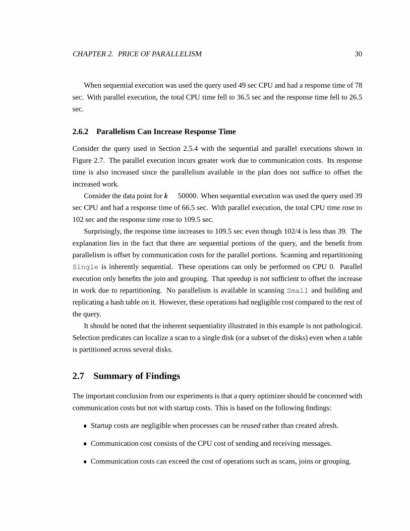
When sequential execution was used the query used 49 sec CPU and had a response time of 78
sec. With parallel execution, the total CPU time fell to 36.5 sec and the response time fell to 26.5
sec.
2.6.2 Parallelism Can Increase Response Time
Consider the query used in Section 2.5.4 with the sequential and parallel executions shown in
Figure 2.7. The parallel execution incurs greater work due to communication costs. Its response
time is also increased since the parallelism available in the plan does not suffice to offset the
increased work.
Consider the data point for k = 50000. When sequential execution was used the query used 39
sec CPU and had a response time of 66.5 sec. With parallel execution, the total CPU time rose to
102 sec and the response time rose to 109.5 sec.
Surprisingly, the response time increases to 109.5 sec even though 102/4 is less than 39. The
explanation lies in the fact that there are sequential portions of the query, and the benefit from
parallelism is offset by communication costs for the parallel portions. Scanning and repartitioning
Single is inherently sequential. These operations can only be performed on CPU 0. Parallel
execution only benefits the join and grouping. That speedup is not sufficient to offset the increase
in work due to repartitioning. No parallelism is available in scanning Small and building and
replicating a hash table on it. However, these operations had negligible cost compared to the rest of
the query.
It should be noted that the inherent sequentiality illustrated in this example is not pathological.
Selection predicates can localize a scan to a single disk (or a subset of the disks) even when a table
is partitioned across several disks.
2.7 Summary of Findings
The important conclusion from our experiments is that a query optimizer should be concerned with
communication costs but not with startup costs. This is based on the following findings:
� Startup costs are negligible when processes can be reused rather than created afresh.
� Communication cost consists of the CPU cost of sending and receiving messages.
� Communication costs can exceed the cost of operations such as scans, joins or grouping.
CHAPTER 2. PRICE OF PARALLELISM 31
Our experiments show that the cost of parallel execution can differ substantially from that of
sequential execution. The cost may be more or even less depending on what data needs to be
communicated.
It is worth observing that the cost of communication relative to the cost of operators is a strong
function of the quality of the implementation. For example if operators are poorly implemented,
communication costs will be relatively low. Further, such a poor implementation may actually lead
to the system exhibiting good scalability! This underlines the fact that scalability must be tested
with respect to the best implementation on a uniprocessor.
An interesting question is how communication can be avoided or its cost reduced. Architec-
tural techniques such as DMA are likely to help to some extent. However, most of the cost of
communications tends to be incurred at software levels that are higher than DMA interfaces. Use
of shared-memory is of limited value since the cost of communication through a shared piece of
memory rises as the number of processors increases.
Chapter 3
JOQR Optimizations
In this chapter1 we develop models and algorithms for the JOQR phase that minimize the total
cost of computing a query. The models take a “macro” view of query execution. They focus on
exploiting physical properties such as the partitioning of data across nodes; determination of the best
combination of methods for computing operators; and fixing the order of joins. “Micro” decisions
about allocation of resources are the responsibility of the subsequent parallelization phase.
We start with a simple model that captures the communication incurred when data needs to be
repartitioned across processors. Minimizing communication is posed as a tree coloring problem
(related to classical Multiway Cut problems [DJP+92]) in which colors represent data partitioning.
We then enhance the model in two ways. Firstly, we generalize colors to represent any collection
of physical properties (such as sort-order, indexes) that can be exploited in computing an operator.
Secondly, we permit each operator to have several alternate methods by which it can be computed.
This allows us to captures effects such as the fact that a Grouping may be computed very efficiently
if the data is partitioned as well as sorted on the grouping attribute.
The final enhancement of the model is to allow joins to be reordered. At the end of the chapter,
we describe several ways in which the algorithms may be used.
It is appropriate to contrast the models and algorithms in this chapter with work in conventional
query optimization [SAC+79]. Besides incorporating communication costs, our contribution is to
show that choosing methods and physical properties can be separated from join ordering. While join
ordering requires exponential time, methods and physical properties can be chosen in polynomial
1Parts of this chapter have been published in the two papersW. Hasan and R. Motwani: Coloring Away Communication in Parallel Query Optimization, VLDB95S. Ganguly, W. Hasan and R. Krishnamurthy: Query Optimization for Parallel Execution, Sigmod92
32
CHAPTER 3. JOQR OPTIMIZATIONS 33
time. Further, join ordering only applies to joins. The algorithms for choosing physical properties
and methods are applicable to any query tree. This opens up new ways of combining the different
aspects of query optimization even for conventional systems.
3.1 A Model for Minimizing Communication
Partitioned parallelism which exploits horizontal partitioning of relations may require data to be
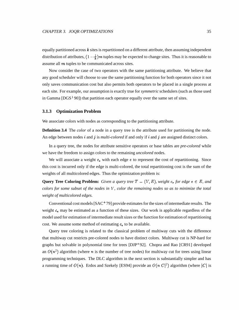
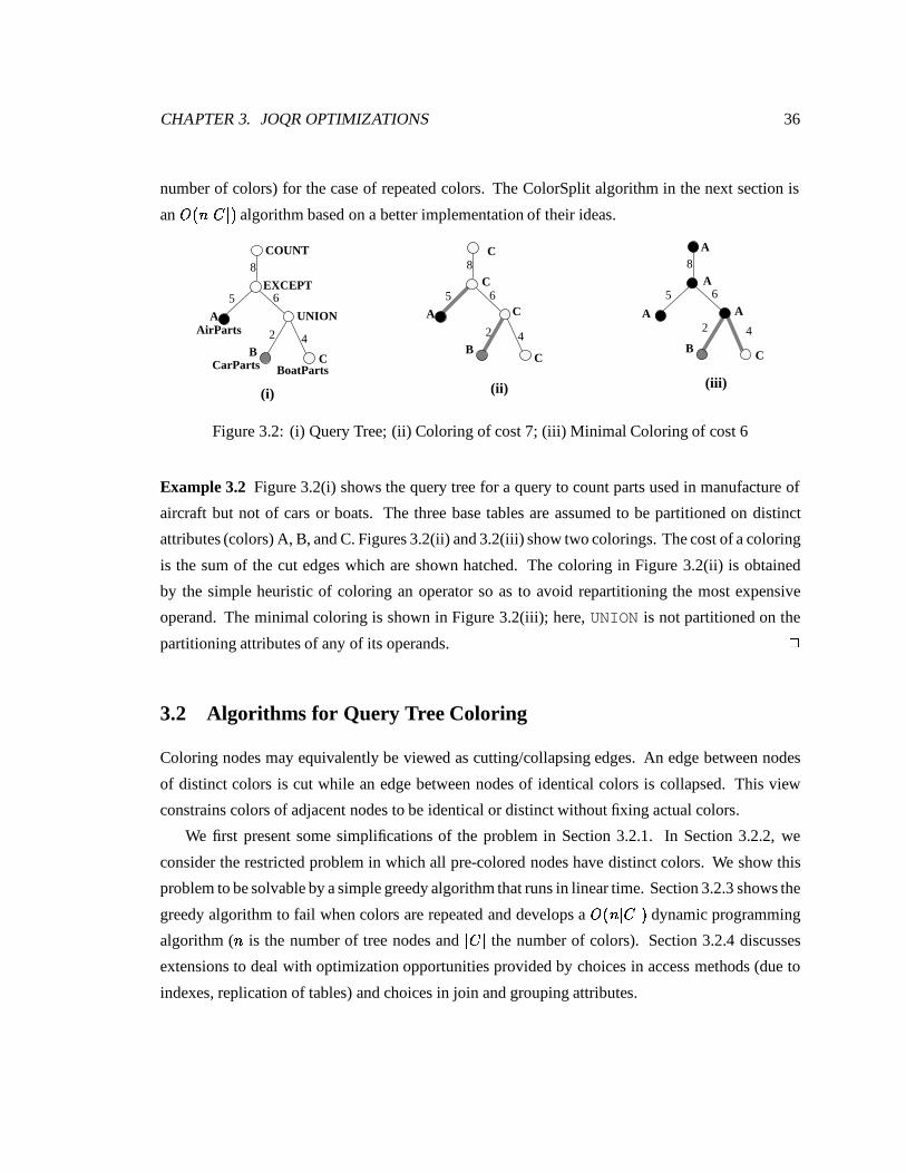
repartitioned among sites thus incurring substantial communication costs.
Example 3.1 Assume tablesEmp(enum,name, areaCode, number) andCust(name,areaCode,
number) are horizontally partitioned on two sites on the underlined attributes. The following query
(in SQL2 [X3H92] syntax) determines the number of employees who are also customers in each
area code. An employee and a customer are guessed to be the same person if they have the same
name and phone number:
Select areaCode, Count(*)
From Cust Intersect (Select name, areaCode, number From Emp)
Group by areaCode;
Figure 3.1 shows two query trees that differ only in how data is repartitioned. Since tuples with
the same areaCode need to come together, GroupBy is partitioned by areaCode. However,
Intersect may be partitioned on any attribute. If we choose to partition it by areaCode,
we will need to repartition the (projected) Emp table. If we partition by name, we will need to
repartition the Cust table as well as the output of Intersect. Thus one or the other query tree
may be better depending on the relative sizes of the intermediate tables. 2
Emp0 : hash(name) mod 2 = 0Cust0 hash(areaCode ) mod 2 = 0
Emp Cust
Intersect
GroupBy
(a) Schema (b) Alternate Query Trees
SIT
E 0
SIT
E 1
Emp Cust
Intersect
GroupBy
Emp1 : hash(name) mod 2 = 1Cust1 hash(areaCode ) mod 2 = 1
(name)(areaCode)
(areaCode) (areaCode)
(areaCode)
(areaCode) (name)
(name)
Figure 3.1: Query Trees: Hatched edges show repartitioning
3.1.1 Partitioning
We begin with a formal definition of partitioning.
CHAPTER 3. JOQR OPTIMIZATIONS 34
Definition 3.1 A partitioning is a pair (a; h) where a is an attribute and h is a function that maps
values of a to non-negative integers.
Given a table T , a partitioning produces fragments T0; : : : ; Tk
For example, the partitioning of Emp in Example 3.1 is represented as (name, hash(name)
mod 2 ). The function hash(name) mod 2 is applied to each tuple of Emp and the tuple placed
in fragment Emp0 or Emp1 depending on whether the function returns 0 or 1.
Partitioning provides a source of parallelism since the semantics of most database operators
allows them to be applied in parallel to each fragment. Suppose S0; : : : ; Sk and T0; : : : ; Tk are
fragments of tables S and T produced by the same partitioning � = (a; h).
Definition 3.2 A unary operator f is partitionable with respect to � if and only if f(S) = f(S0)[: : : [ f(Sk). A binary operator f is partitionable with respect to � if and only if f(S; T ) =
f(S0; T0) [ : : :[ f(Sk; Tk).
Definition 3.3 An attribute sensitive operator is partitionable only for partitionings that use a
distinguished attribute. An attribute insensitive operator is partitionable for all partitionings.
The equation S ./ T = [i(Si ./ Ti) holds only if both S and T are partitioned on the (equi-
)join attribute. Thus join is attribute sensitive. Similarly, grouping is attribute sensitive since it
requires partitioning by the grouping attribute. UNION, INTERSECT and EXCEPT (set difference),
aggregation, selection and projection are attribute insensitive. External functions and predicates
may be either sensitive or insensitive.
3.1.2 Repartitioning Cost
Communicating tuples between operators that use different partitionings requires redistributing
tuples among sites. Some percentage of tuples remain at the same site under both partitionings and
therefore do not need to be communicated across sites. We believe that the crucial determinant of
the extent of communication cost, given a “good” scheduler, is the attribute used for partitioning.
We argue the following all or nothing assumption to be reasonable.
Good Scheduler Assumption: If two communicating operators use the same partitioningattribute,
no inter-site communication is incurred. If they use distinct partitioning attributes then all tuples
need to be communicated across sites.
Consider the case of two operators with different partitioning attributes. The greatest savings in
communication occur if the two operators use the same set of processors. If a table with m tuples
CHAPTER 3. JOQR OPTIMIZATIONS 35
equally partitioned across k sites is repartitioned on a different attribute, then assuming independent
distribution of attributes, (1� 1k)m tuples may be expected to change sites. Thus it is reasonable to
assume all m tuples to be communicated across sites.
Now consider the case of two operators with the same partitioning attribute. We believe that
any good scheduler will choose to use the same partitioning function for both operators since it not
only saves communication cost but also permits both operators to be placed in a single process at
each site. For example, our assumption is exactly true for symmetric schedulers (such as those used
in Gamma [DGS+90]) that partition each operator equally over the same set of sites.
3.1.3 Optimization Problem
We associate colors with nodes as corresponding to the partitioning attribute.
Definition 3.4 The color of a node in a query tree is the attribute used for partitioning the node.
An edge between nodes i and j is multi-colored if and only if i and j are assigned distinct colors.
In a query tree, the nodes for attribute sensitive operators or base tables are pre-colored while
we have the freedom to assign colors to the remaining uncolored nodes.
We will associate a weight ce with each edge e to represent the cost of repartitioning. Since
this cost is incurred only if the edge is multi-colored, the total repartitioning cost is the sum of the
weights of all multicolored edges. Thus the optimization problem is:
Query Tree Coloring Problem: Given a query tree T = (V;E), weight ce for edge e 2 E, and
colors for some subset of the nodes in V , color the remaining nodes so as to minimize the total
weight of multicolored edges.
Conventional cost models [SAC+79] provide estimates for the sizes of intermediate results. The
weight ce may be estimated as a function of these sizes. Our work is applicable regardless of the
model used for estimation of intermediate result sizes or the function for estimation of repartitioning
cost. We assume some method of estimating ce to be available.
Query tree coloring is related to the classical problem of multiway cuts with the difference
that multiway cut restricts pre-colored nodes to have distinct colors. Multiway cut is NP-hard for
graphs but solvable in polynomial time for trees [DJP+92]. Chopra and Rao [CR91] developed
an O(n2) algorithm (where n is the number of tree nodes) for multiway cut for trees using linear
programming techniques. The DLC algorithm in the next section is substantially simpler and has
a running time of O(n). Erdos and Szekely [ES94] provide an O(njCj2) algorithm (where jCj is
CHAPTER 3. JOQR OPTIMIZATIONS 36
number of colors) for the case of repeated colors. The ColorSplit algorithm in the next section is
an O(njCj) algorithm based on a better implementation of their ideas.
5
2 4
(ii) (iii)
COUNT
EXCEPT
UNION
CarParts BoatParts
AirPartsA
B C
6
8
5
2 4
A
B
6
8
5
2 4
A
B C
6
8
(i)
C
C
C
C
A
A
A
Figure 3.2: (i) Query Tree; (ii) Coloring of cost 7; (iii) Minimal Coloring of cost 6
Example 3.2 Figure 3.2(i) shows the query tree for a query to count parts used in manufacture of
aircraft but not of cars or boats. The three base tables are assumed to be partitioned on distinct
attributes (colors) A, B, and C. Figures 3.2(ii) and 3.2(iii) show two colorings. The cost of a coloring
is the sum of the cut edges which are shown hatched. The coloring in Figure 3.2(ii) is obtained
by the simple heuristic of coloring an operator so as to avoid repartitioning the most expensive
operand. The minimal coloring is shown in Figure 3.2(iii); here, UNION is not partitioned on the
partitioning attributes of any of its operands. 2
3.2 Algorithms for Query Tree Coloring
Coloring nodes may equivalently be viewed as cutting/collapsing edges. An edge between nodes
of distinct colors is cut while an edge between nodes of identical colors is collapsed. This view
constrains colors of adjacent nodes to be identical or distinct without fixing actual colors.
We first present some simplifications of the problem in Section 3.2.1. In Section 3.2.2, we
consider the restricted problem in which all pre-colored nodes have distinct colors. We show this
problem to be solvable by a simple greedy algorithm that runs in linear time. Section 3.2.3 shows the
greedy algorithm to fail when colors are repeated and develops a O(njCj) dynamic programming
algorithm (n is the number of tree nodes and jCj the number of colors). Section 3.2.4 discusses
extensions to deal with optimization opportunities provided by choices in access methods (due to
indexes, replication of tables) and choices in join and grouping attributes.
CHAPTER 3. JOQR OPTIMIZATIONS 37
3.2.1 Problem Simplification
The problem of coloring a tree can be reduced to coloring a set of trees which have the special
property that all interior nodes are uncolored and all leaves are pre-colored. This follows from the
following observations which imply that colored interior nodes may be split into colored leaves,
and uncolored leaves may be deleted.
(Split) A colored interior node of degree d may be split into d nodes of the same color and each
incident edge connected to a distinct copy. This decomposes the problem into d sub-problems
which can be solved independently.
(Collapse) An uncolored leaf node may be collapsed into its parent. This gives it the same color
as its parent which is minimal since it incurs zero cost.
Nested-Loops Join hp : X; s : Y; i : nonei hp : X; s : Y; i : �i hp : X; s : �; i : Xi Join predicate on X
Sort-Merge Join hp : X; s : X; i : nonei hp : X; s : X; i : �i hp : X; s : X; i : �i Join predicate on X
Hybrid-Hash Join hp : X; s : Y; i : nonei hp : X; s : Y; i : �i hp : X; s : �; i : �i Join predicate on X
Hash Grouping hp : X; s : none; i : nonei hp : X; s : �; i : �i X is a grouping attributeSort Grouping hp : X; s : X; i : nonei hp : X; s : X; i : �i X is a grouping attributeHash Intersect hp : X; s : none; i : nonei hp : X; s : �; i : �i hp : X; s : �; i : �i
Table 3.1: Examples of Input-Output Constraints
Our goal is to devise an abstract cost model that is compatible with classical cost models. Such
classical models typically consists of two parts: (a) estimation of statistics (such as size, number
of unique values in columns) for intermediate results; and, (b) estimation of cost of an operator
given statistics and physical properties of operands. Our goal is not to provide new formulas but to
provide abstractions that make it possible to reason with formulas provided by existing models in a
more general manner.
Definition 3.8 Rs is the set of statistics for table R. Rs depends only on the contents of table R,
not on how it is physically stored.
Definition 3.9 recolor(Rs; cold; cnew) is the cost of re-coloring table R from cold to cnew.
Definition 3.10 inpCol(s; A; j) is the color pattern needed by strategy s for input j for the output
to be of color pattern A.
CHAPTER 3. JOQR OPTIMIZATIONS 47
Example 3.8 The color required for the first input of the nested-loops join in the first query tree
of Figure 3.8 is cnew = hp : dep#; s : city; i : �i. Since the output color (call it cold) of Emp
differs in partitioning attribute, recolor(R; cold; cnew) is the cost of repartitioningEmp on the city
attribute. 2
The cost of an annotated query tree is the sum of the costs of all operators. The cost of an
operator consists of re-coloring the inputs to have colors needed by the chosen strategy plus the
cost of the strategy itself. Suppose the root of tree T uses strategy s and has output color a. Let
c0j = inpCol(s; a; j), the color required by strategy s for the j’th input. Let T have k immediate
subtrees T1; : : : ; Tk such that Tj produces table Rj with color cj .
Cost(T ) = StrategyCost(s; Rs1; : : : ; R
sk) +
kXj=1
recolor(Rsj; cj; c
0j) +
kXj=1
Cost(Tj)
If T is a leaf, we take its cost as zero since we count the cost of accessing operands as part of
the cost of a strategy. Since the output of a query is always shipped to an application, the root of
any query tree will be a unary operator that achieves the shipping. By convention, we will omit
showing this operator2.
Observe that no restriction is placed on the form of the StrategyCost() or recolor() functions.
This allows, for example, non-linear terms such as logarithms, product and division that do occur
in the classical System R [SAC+79] cost model.
3.4 Extension of ColorSplit for Methods and Physical Properties
We will now develop an extension of ColorSplit that given a tree with colors for the leaf nodes finds
a minimal-cost strategy as well as input and output colors for each interior node.
Definition 3.11 Optc(i; A) is defined to be the minimal cost of the subtree rooted at node i such that
i has output color A. OptcStrategy(i; A) is defined to be the strategy that achieves this minimal
value (pick any one strategy if several are minimal).
For a leaf node i, Optc(i; A) = 0 if i is pre-colored with a color compatible with A and 1otherwise. We will treat OptcStrategy(i; A) as undefined for leaf nodes.
2Consider a query that simply scans a table. It will have a query tree consisting of a Ship with Scan as the onlychild. Observe that the cost of scanning data is counted as part of Ship.
CHAPTER 3. JOQR OPTIMIZATIONS 48
Definition 3.12 Strategies(i; A) is the set of strategies applicable to the operator represented by
node i and whose input-output constraint permits A as an output color.
The following is a generalization of Lemma 3.3. Let node i have children �1; : : : ; �k. Suppose
the subtree rooted at �j computes table Rj as its output. The minimum cost of the tree rooted at i
such that i has output color A is obtained by trying out all strategies capable of producing output
color A. The lemma shows that for any such strategy s, the lowest cost is achieved by individually
minimizing the cost of each input.
Lemma 3.6 For a leaf node i, Optc(i; A) is 0 if i has a color compatible with A and1 otherwise.
For non-leaf node i, Optc(i; A) obeys the following recurrence.
Optc(i; A) = mins2S [StrategyCost(s; Rs1; : : : ; R
sk)+Pk
j=1 minc2C [Optc(�j; c) + recolor(Rsj; c; inpCol(s;A; j))]]
where S = Strategies(i; A)
OptcStrategy(i; A) is some strategy for which the minima is achieved.
Using the lemma, the following algorithm computes Optc and OptcStrategy by a bottom-up
followed by a subsequent top-down pass that extracts optimal colors and strategies.
Algorithm 3.4 Algorithm ExtendedColorSplit
1. for each node i in postfix order do step 2
2. Use Lemma 3.6 to computeOptc(i; a) and OptcStrategy(i; a) for each color a 2 C
3. Let r be the root and a a color s.t. Optc(r; a) � Optc(r; c) for all colors c 2 C
4. Optimal color for r is a and optimal strategy is OptcStrategy(r; a)
5. for each non-root node in prefix order do step 6
6. compute optimal colors and strategies by top-down pass applying Lemma 3.6 in reverse.
The algorithm has a worst-case running time of nSjCj2 where S is the number of strategies,
jCj the number of allowable colors and n the number of nodes in the tree.
Since n and S are typically small, the running time of the algorithm is dependent on jCj. jCjcan become large when we permit the extensions discussed in section 3.2.4. The magnitude of jCjmay be kept small by observing (1) no strategy yields an output relation with an index. Thus only
2 components of the triple for colors are relevant for interior nodes (2) only colors that might be
useful to subsequent operator need to be considered.
CHAPTER 3. JOQR OPTIMIZATIONS 49
3.5 Model With Join Ordering
We now show an example of how repartitioning costs interact with the order of joins.
EmpSkillsEmp
Skills
( emp# )
( skill# )
( emp# )
( emp# )
( skill# )
EmpSkills
Emp
Skills
( emp# )
( skill# ) ( emp# )
( emp# )
( skill# )
Figure 3.9: Interaction of Repartitioning with Order of Joins
Example 3.9 Suppose the tables Emp(emp#, city), EmpSkills(emp#, skill#), and
Skills(skill#, skilltype) are partitioned by the underlined attributes. The following
query finds employees who live in Palo Alto and have analytical skills.
Select e from Emp e, EmpSkills es, Skills s
Where e.emp# = es.emp# and es.skill# = s.skill# and
s.skilltype = Analytical and e.city = Palo Alto
Figure 3.9(i) and (ii) shows two alternate query trees. The trees use different join orders and
incur different repartitioning costs. If “s.skilltype = analytical” is a highly selective
predicate, the second tree may achieve a low cost due to the small size of the intermediate table
(Skills ./ EmpSkills). However, the first tree avoids the cost of repartitioning the possibly
very large EmpSkills table. Thus repartitioning cost impacts the ordering of joins. Figure 3.9(iii)
illustrates the details of the strategy annotations for join operations. 2
Commercially adopted solutions to join ordering are typically variations of the System R
algorithm [SAC+79]. Our goal is to combine the basic ideas from this algorithm with the ColorSplit
algorithm. We will start by developing an abstraction of some aspects of the System R style dynamic
programming. This will us to understand and analyze the basic ideas while ignoring many details
of the actual algorithm.
3.5.1 Join Ordering Without Physical Properties
Definition 3.13 A join tree is an annotated query tree in which all interior nodes represent 2-way
join operations and leaves represent tables.
CHAPTER 3. JOQR OPTIMIZATIONS 50
Since join operations are associative and commutative, they may be performed in any order.
Given a SPJ query on tables T1; : : : ; Tn, the join ordering problem is to find a minimal cost join tree
for computing the query. A join tree fixes the order of joins in addition to the strategy for each join.
We will use a nested list notation to represent join trees. For example, the tree of figure 3.9(iii) may
be represented as [s2; [s1; Skills; EmpSkills]; Emp]
For simplicity, we first consider the case when re-coloring has zero cost. In other words, physical
properties do not make a difference to cost and we have:
Cost(T ) =
8<: 0 if T is a leaf
StrategyCost(s; Rsl ; R
sr) + Cost(Tl) + Cost(tr) if T = [s; Tl; Tr]
The following lemma follows from the structure of the cost formula and implies that any subtree
of an optimal query tree must be an optimal query tree for the corresponding sub-query.
Lemma 3.7 If OptP lan(Q) = [s; Tl; Tr] and Q = Ql [Qr where Tl computes the sub-query over
Ql and Tr over Qr, then OptP lan(Ql) = Tl and OptP lan(Qr) = Tr
This lemma leads to the following dynamic programming algorithm:
Algorithm 3.5 Algorithm JO (Join Ordering)
Input: SPJ query on tables T = fT1; : : : ; TngOutput: Optimal join tree.
1. for i = 1 to n do OptP lan(fTig) = Ti
2. for i= 2 to n do step 3
3. for each Q � T s.t. jQj = i do steps 4 and 5
4. bestCost = 15. for each Ql 6= ;, Qr 6= ; s.t. Q = Ql [Qr do steps 6 and 7
6 Let Rsl ; R
sr be statistics for tables computed by queries Ql; Qr
7. for each join strategy s do steps 8 to 11
8. if StrategyCost(s; Rsl ; R
sr) < bestCost then
9. bestCost = StrategyCost(s; Rsl ; R
sr)
10. OptP lan(Q) = [s; OptP lan(Ql); OptP lan(Qr)]
11. end if
The algorithm has a running time of O(3n). Since plans for all subsets of Q are cached, and
a plan for i tables has storage cost proportional to i, the space requirements of the algorithm are
CHAPTER 3. JOQR OPTIMIZATIONS 51
O(n2n). A brute force enumeration of all trees would run inO(2n!=n!) time but require onlyO(n)
space (for 1 plan).
Often systems choose a restricted class of shapes of join trees. A popular restriction is left-deep
trees that require the left child of any interior node to be a leaf. This cuts the number of trees to n!
and the algorithm runs in O(n2n) time.
3.5.2 Join Ordering With Physical Properties
Suppose strategy s requires input colors c0
l and c0
r. Suppose sub-plan (subtree) Tl produces table Rl
with color cl (Rr and cr for sub-plan Tr).
Cost(T ) =
8>>><>>>:
0 if T is a leaf
recolor(Rsl ; cl; c
0
l) + recolor(Rsr; cr; c
0
r)+
StrategyCost(s; Rsl ; R
sr) + Cost(Tl) + Cost(Tr) if T = [s; Tl; Tr]
Let Optc(Q;A) be the cost of an optimal join tree for the set of tables Q such that the output
has physical property A.
Lemma 3.8 Optc(Q; a) obeys the following recurrence:
Optc(Q; a) = minQl;Qr[mins2S [StrategyCost(s; Ql; Qr)
+mina2C [Optc(Ql; a) + recolor(Qsl ; a; inpCol(s; a; 1))]
+mina2C [Optc(Qr; a) + recolor(Qsr; a; inpCol(s; a; 2))]]]
where Ql and Qr are all sets such that Q = Ql [Qr, Ql 6= ;, Qr 6= ; and S is the set of strategies
that produce property a.
Algorithm 3.6 Algorithm JOP (Join Ordering With Physical Properties)
Input: An SPJ query on tables T = fT1; : : : ; TngOutput: An optimal join tree.
1. for i = 1 to n do step 2
2. Optc(Ti; a) =
8<: 0 Ti has access method with physical property a
1 otherwise
3. for i = 2 to n do step 4
4. for each Q � T s.t. jQj = i do steps 5 and 6
CHAPTER 3. JOQR OPTIMIZATIONS 52
External function
SPJ
SPJ
EXCEPT
INTERSECTUNION
T1T2 T3 T4
Figure 3.10: Decomposition of a complex query
5. Optc(Q; a) = 1 for each physical property a 2 C
6. for each Ql 6= ;, Qr 6= ; s.t. Q = Ql [Qr do steps 7 and 8
7. Let Rsl ; R
sr be statistics for tables computed by queries Ql; Qr
8. for each physical property a 2 C do step 9
9. for each strategy s that can produce property a do steps 10 and 11
10. Let scost = StrategyCost(s; Rsl ; R
sr), a
0
l = inpCol(s; a; 1) and a0
r = inpCol(s; a; 2)
11. for each physical property al 2 C, ar 2 C do steps 12 to 16
12. Let newcost = scost +Optc(Ql; al) + recolor(Rsl ; al; a
17. return Mina2COptP lan(T ; a)A complex query may be decomposed into SPJ queries connected by other operators(Figure 3.10).
We remark that it is possible to integrate the JOP and ExtendedColorSplit algorithms in a straight-
forward manner to produce an optimal annotated query tree. The tree is optimal with respect to all
allowed orderings within SPJ boxes and all possible annotations of nodes.
3.6 Usage of Algorithms
There are several ways in which the algorithms developed in this chapter may be used. One
possibility is to use ExtendedColorSplit as a post-pass to a conventional optimizer. This has two
CHAPTER 3. JOQR OPTIMIZATIONS 53
advantages. First, no modifications is required to existing optimizers. Secondly, ExtendedColorSplit
runs in polynomial time. The disadvantage is that the query trees will have optimal annotations
given the join orders produced by the conventional optimizer. The second possibility is to produce
optimal join order as well as annotation by using the integration of the JOP and ExtendedColorSplit
as a replacement for a conventional optimizer.
Chapter 4
Scheduling Pipelined Parallelism
In this chapter1, we focus on the problem of scheduling a pipelined operator tree, which is an
operator tree in which all edges are pipelining edges. Pipelined parallelism permits all operators in
such a tree to run concurrently. Scheduling such trees poses a parallelism-communication trade-off.
A producer and a consumer operator must either communicate data across processors to benefit
from and run on distinct processors, or they must share a processor but save communication.
We will measure the quality of scheduling algorithms by their performance ratio [GJ79] which
is the ratio of the response time of the generated schedule to that of the optimal. Our goal is to
devise algorithms that are near-optimal in the sense that the average performance ratio should be
close to 1 and the worst performance ratio should be a small constant.
We start by defining the problem more precisely. We then develop and analyze several algorithms
followed by an experimental comparison.
4.1 Problem Definition
Definition 4.1 Given p processors and an operator tree T = (V;E), a schedule is a partition of V ,
the set of nodes, into p sets F1; : : : ; Fp with set Fk allocated to processor k.
The cost of executing Fk is the cost of executing all nodes in Fk plus the cost for communicating
with nodes on other processors. It is thus the sum of the weights of all nodes in Fk and the weights
1Parts of this chapter have been published in the two papersW. Hasan and R. Motwani: Optimization Algorithms for Exploiting the Parallelism-Communication Tradeoff in PipelinedParallelism, VLDB94C. Chekuri, W. Hasan and R. Motwani: Scheduling Problems in Parallel Query Optimization, PODS95
54
CHAPTER 4. SCHEDULING PIPELINED PARALLELISM 55
PROBE(h1)
PROBE(h2)
MERGE
SCAN(E) SCAN(D)
7
1
5
1
14
23
3
8
108
time
Idle fraction [0.2]
Idle fraction [0.2]
Pro
cess
or1
Pro
cess
or2
Pro
cess
or3
0 10
(A) Schedule (B) Gantt Chart
F1 F2
F3 PROBE(h1) [0.8]
PROBE(h2) [0.7]
SCAN(D) [0.3]
MERGE [0.5]
SCAN(E) [0.3]
Figure 4.1: A pipelined schedule and its execution
of all edges that connect a node within Fk to a node outside. For convenience, we define cij = 0 if
there is no edge from i to j.
Definition 4.2 The load Lk on processor k isP
i2Fk [ti +P
j =2Fk cij ].
The response time, L, of a schedule may be derived by observing that pipelining constraints
force all operators in a pipeline to start simultaneously (time 0) and terminate simultaneously at time
L. Fast operators are forced to “stretch” over a longer time period by the slow operators. Suppose
operator i is allocated to processor k and uses fraction fi of the processor. The pipelining constraint
is then:
fi =1L[ti +
Xj =2Fk
cij ] for all operators i 2 V (4.1)
The utilization of a processor is the sum of utilizations of the operators executing on it. Since
at least one processor must be saturated (otherwise the pipeline would speed up):
max1�k�p
[Xi2Fk
fi] = 1
) L = max1�k�p
[Xi2Fk
[ti +Xj =2Fk
cij ]] = max1�k�p
Lk using equation (4.1)
Example 4.1 Figure 4.1(a) shows a schedule by encircling the sets Fk. The cost of each set is
underlined. For example fPROBE(h1)g costs 8 by adding up its node weight (7) and the weight of
the edge (1) connecting it to its child. Observe that we show edges as undirected since the parallel
constraint represented by pipelining edges is symmetric. Figure 4.1(b) shows a Gantt chart of the
execution specified by the schedule. The fraction of the processor used by each operator in shown
in parenthesis. 2
The pipelined operator tree scheduling (POT) problem may now be stated as follows:
CHAPTER 4. SCHEDULING PIPELINED PARALLELISM 56
Input: Operator Tree T = (V;E)with positive real weights ti for each node i 2 V and cij for
each edge (i; j) 2 E; number of processors p
Output: A schedule with minimal response time i.e., a partition of V into F1; : : : ; Fp that
minimizes max1�l�pP
i2Fl[ti +
Pj =2Fl
cij ].
Definition 4.3 If F is a set of operators, cost(F ) is the load on a processor that computes F .
cost(F ) =P
i2F [ti +P
j =2F cij ].
Since the special case in which all edge weights are zero is multiprocessor scheduling [GJ79,
GLLK79], POT is NP-hard. Since the number of ways of partitioning n elements into k disjoint
non-empty sets is�nk
(which denotes Stirling numbers of the second kind) [Knu73], the number
of distinct schedules for a tree with n nodes on p processors isP
1�k�p�nk
. This number is about
1:2� 105 for n = p = 10 and 5:0� 1013 for n = p = 20, thus ruling out enumerative approaches
to the problem.
A natural question is whether multiprocessor scheduling algorithms such as LPT may be adapted
for POT. Multiprocessor scheduling is the problem of scheduling independent jobs with known
running times on a set of processors. LPT assigns the job with the largest running time to the least
loaded processor, repeating this step until all jobs are assigned. For p processors, LPT has a worst
case performance ratio of 43 � 1
3p [Gra69].
LPT may be applied to POT by simply using the cost of each node (i.e. the node weight plus
weights of all incident edges) as its running time. This Naive LPT algorithm performs poorly since
it is unaware of the tradeoff between parallelism and communication. Consider two operators each
of weight t connected by an edge of weight c. To obtain a schedule for 2 processors, Naive LPT
will consider the cost of each operator to be t + c and place them on separate processors resulting
in a schedule with a response time of t + c. LPT never saves communication cost by placing both
operators on a single processor which would achieve a response time of 2t. Since cheap operators
and expensive communication can make the ratio t+c2t arbitrarily large, the worst case performance
ratio of Naive LPT is unbounded.
Our algorithms will use the operations of cutting and collapsing edges that correspond to
decisions to place adjacent nodes on the same or different processors.
Definition 4.4 Collapse(i; j) modifies a tree by replacing nodes i and j by a single new node i0
with weight ti0 = ti + tj . Edges that were connected to either i or j are instead connected to i0.
Definition 4.5 Cut(i; j) modifies a tree by deleting edge (i; j) and adding its weight to that of the
nodes i and j, i.e. tnewi = toldi + cij and tnewj = toldj + cij .
CHAPTER 4. SCHEDULING PIPELINED PARALLELISM 57
If a schedule places both i and j on processor k, the load on all processors is invariant when
i and j are collapsed, and the new node is placed on processor k. If a schedule places i and j on
distinct processors, the load is invariant when (i; j) is cut.
Our analysis with often consider the following two special cases.
Definition 4.6 A star is a tree with one non-leaf node. A path is a tree with two leaves.
4.2 Identifying Worthless Parallelism
In this section we investigate the tradeoff between parallelism and communication cost and de-
velop the GreedyChase algorithm that “chases” down and removes parallelism that is “worthless”
irrespective of the number of processors.
We start by characterizing worthless edges whose communication overhead is relatively high
enough to exceed any benefits from parallelism. We the identify a class of trees that we call
monotone. Such trees have no worthless parallelism in the sense that maximal use of parallelism
is in fact optimal. We show that repeatedly collapsing worthless edges results in a monotone tree.
Finally, we provide lower bounds on schedules for monotone trees.
4.2.1 Worthless Edges and Monotone Trees
In Figure 4.1, the cost incurred by MERGE in communicating with SCAN(E) is 4 seconds which
exceeds the cost of SCAN(E) itself. It is thus always better for the processor executing MERGE to
execute SCAN(E) locally rather than communicate with it. We now generalize this observation.
Definition 4.7 An edge eij is worthless if and only if (cij � ti +P
k 6=j cik) or (cij � tj +Pk 6=i cjk).
The following theorem shows that our definition of worthless indeed captures edges whose high
communication cost offsets the advantage of parallel execution.
Theorem 4.1 Given p processors and an operator tree T with worthless edge (i; j), there exists an
optimal schedule of T for p processors in which nodes i and j are assigned to the same processor.
Proof: We prove the theorem by showing that given a worthless edge (i; j) and an optimal
schedule S, we can generate another schedule S 0 (for the same number of processors) with no higher
response time in which (i; j) is collapsed.
CHAPTER 4. SCHEDULING PIPELINED PARALLELISM 58
Let Fp and Fq be the sets of nodes assigned to processors p and q in S such that i 2 Fp and
j 2 Fq. Since (i; j) is worthless, without loss of generality we may assume
cij � tj +Xk 6=i
cjk (4.2)
We show S 0 to consist of S modified by moving j from q to p. This move changes the loads only
on p and q and we show that neither load can increase.
Moving j onto processor p increases the load on p by at most [tj +P
k2(V�Fp) cjk] � cij ,
since p saves the cost of the edge between i and j, but incurs the additional cost of j as well as
j communicating with nodes other than those assigned to p. Observing thatP
k2(V�Fp) cjk �Pk 6=i cjk, Equation 4.2 shows this increase cannot be positive.
Removing j from processor q increases the load on q by �cij � tj +P
k2Fq cjk, since q saves
the cost of j, and j communicating with i, but must now incur the cost of the remaining nodes of Fq
communicating with j. Observing thatP
k2Fq cjk �P
k 6=i cjk , Equation 4.2 shows this increase
cannot be positive. 2
Definition 4.8 An operator tree is monotone if and only if any connected set of nodes, X , has a
lower cost than any connected superset, Y , i.e., if X � Y then cost(X) < cost(Y ).
We now establish an important connection between worthless edges and monotone trees. The
following theorem allows us to transform any tree into a monotone tree by collapsing all worthless
edges. More importantly, we can schedule the monotone tree rather than the original tree. This
follows since collapsing worthless edges does not sacrifice optimality (Theorem 4.1) and the
schedule for the original tree can be recovered from the schedule for the transformed tree.
Theorem 4.2 A tree is monotone if and only if it has no worthless edges.
Proof: [WORTHLESS EDGE IMPLIES NON-MONOTONICITY]
Assume edge (i; j) is a worthless edge. Without loss of generality, we assume
cij � tj +Xk 6=i
cjk (4.3)
We show cost(fig) � cost(fi; jg) and hence the tree is not monotone.
cost(fig) = ti +Xk
cik
= ti + cij +Xk 6=j
cik
� ti + (tj +Xk 6=i
cij) +Xk 6=j
cik by Equation 4.3
= cost(fi; jg)
CHAPTER 4. SCHEDULING PIPELINED PARALLELISM 59
[NON-MONOTONICITY IMPLIES WORTHLESS EDGE]
If a tree is not monotone, there must be connected sets X and Y such that X � Y with cost(X) �cost(Y ). Since X and Y are both connected sets, it must be possible to arrange the nodes in Y �X
in a sequence v1; : : : ; vm such that Y can be created from X by adding these nodes one by one
and guaranteeing a connected set at all steps. That is, we progress through sets F0; F1; : : : ; Fm
with Fi = F0 [ fv1; : : : ; vig being a connected set and with F0 = X and Fm = Y . Since
cost(F0) � cost(Fm), there must be some vertex v�, such that cost(F��1) � cost(F�). Since
both F��1 and F� are connected but acyclic sets, v� is connected to exactly one node inF��1. Call
that node �.
cost(F�) = cost(F��1) + t� � c�� +Xj 6=�
c�j
Using cost(F��1) � cost(F�), we can conclude t� +P
j 6=� c�j � c�� which proves (�; �) to be
a worthless edge. 2
4.2.2 The GreedyChase Algorithm
Algorithm 4.1 The GreedyChase Algorithm
Input: An operator tree
Output: A monotone operator tree
1. while there exists some worthless edge (i; j)
2. Collapse(i,j)
3. end while
Since each collapse reduces the number of nodes, GreedyChase must terminate. The check for
the existence of a worthless edge is the crucial determinant of the running time. When a worthless
edge is collapsed, adjacent edges may turn worthless and thus need to be rechecked. The algorithm
may be implemented to run in time O(nd), where n is the number of nodes and d is the maximum
degree of any node. Experimentally, the running time of our implementation of GreedyChase was
virtually linear in n.
We remark that even though the order in which new edges turn worthless may depend on the
order of edge collapses, the monotone tree for an operator tree is unique.
CHAPTER 4. SCHEDULING PIPELINED PARALLELISM 60
4.2.3 Lower Bounds
We will use GreedyChase as a pre-processing step in all our algorithms. The following lower
bounds will be useful in analyzing the performance ratios of our algorithms.
Lemma 4.1 Let Ri = [ti +P
j2V cij ] be the net weight of node i. The response time of any
schedule (independent of number of processors) for a monotone operator tree has a lower bound of
R = maxi2V Ri.
Proof: It suffices to show ti +P
j2V cij to be a lower bound for any node i. Suppose Y
is the set of all nodes that are assigned the same processor as i. Y may be decomposed into
maximal connected sets Y1; : : : ; Yq. Suppose i 2 Y�. Since cost(Y ) =P
j cost(Yj), we have
cost(Y ) � cost(Y�). By definition of monotone trees, cost(Y�) � cost(fig). Thus, the load on
the processor executing i is at least cost(fig) which is ti +P
j2V cij . 2
Lemma 4.2 The response time of a p processor schedule for any operator tree (monotone or not)
has a lower bound of W = W=p where W =P
i ti is the total node weight.
Proof: The total load is at least the sum of the node weights and some processor must have at
least the average load. 2
4.3 The Modified LPT Algorithm
The modified LPT algorithm consists of running GreedyChase followed by LPT.
Example 4.2 Figure 4.2(A) shows traces the collapse of worthless edges by GreedyChase. Note
that edges may turn worthless as a result of other collapses. For two processors, modified LPT
produces schedule (B) with response time 11. Naive LPT on the other hand may produce schedule
(C) with response time 25. 2
Modified LPT performs well when the LPT stage receives a monotone tree that is star-shaped.
Edges in a star have low communication costs since the weight of an edge cannot exceed the weight
of the incident leaf without making the edge worthless.
Theorem 4.3 For trees that result in monotone stars, the worst-case performance ratio of the
modified LPT algorithm is less than 2 + 1p. Examples exist that achieve a ratio of 2.
Proof: Consider a star in which the center node, labeled 0, is connected to n� 1 nodes labeled
1; : : : ; n� 1. Let ci be the weight of the edge from node 0 to node i. If all edges are cut, we get
n jobs. The job created from the center has weight �0 = t0 +P
1�i<n ci and the remaining n� 1
jobs have weights �i = ti + ci for i = 1; : : : ; n� 1.
Suppose LPT schedules these jobs to give a response time of L. Let j be the node that when
scheduled caused the load on some processor to reach L. Since LPT assigns a job to the least loaded
processor, the load on all processors must have been at least L� �j when j was assigned. Thus the
total load on all processors has to be at least (L� �j)p+ �j .
(L� �j)p+ �j �X
0�i<n
�i
L � (1� 1p)�j +
1p
X0�i<n
�i
= (1� 1p)�j +
1p[X
0�i<n
ti + 2X
0�i<n
ci]
The above steps are analogous to a standard analysis of the LPT algorithm. We can now exploit a
property particular to stars. Since all edges are incident with node 0,P
1�i<n ci < �0.
L < (1� 1p)�j + (
X0�i<n
ti)=p+2p�0
Since the star is monotone, by Lemmas 4.1 and 4.2, both �j and (Pti)=p are lower bounds on
the optimal response time Lopt. Thus we conclude L=Lopt < 2 + 1p
.
A ratio of 2 is achieved by a star consisting of (p+1) nodes. The center with weight 1 is
connected by edges with weight 0 to (p-1) nodes with weight 2, and by an edge of weight 1� � to
a node of weight 1. The optimal schedule achieves a response time of 2 by placing the two nodes
of weight 1 on the same processor and the remaining p� 1 nodes on distinct processors. The LPT
CHAPTER 4. SCHEDULING PIPELINED PARALLELISM 62
1+ε 1+εε ε ε ε1 1 1 1 1. . .
Figure 4.3: Example with Performance ratio = n=p for Modified LPT
stage of Modified LPT gets (p � 1) nodes of weight 2 and 2 nodes of weight 2 � �. It therefore
produces a schedule with response time 4� 2�. 2
The algorithm is still oblivious to the tradeoff between parallelism and communication. Edges
in a monotone path can have high weights. The algorithm does not attempt to save heavy edges by
assigning the incident nodes to the same processor.
Lemma 4.3 The worst-case performance ratio of modified LPT is unbounded for paths.
Proof: Figure 4.3 shows a monotone path for which the LPT phase receives n jobs each of
weight 2 + �. It can produce a schedule with a response time of (2 + �)n=p � 2n=p. The optimal
is obtained by cutting the path into p pieces of equal length thus obtaining a response time of
2 + dn=pe� � 2 and a performance ratio of n=p. 2
4.4 Connected Schedules
A connected schedule requires the nodes assigned to any processor to be a connected set. This
restriction is equivalent to only considering schedules that incur communication cost on p�1 edges
(the minimal possible number) when using p processors.
A practical reason for investigating connected schedules is execution efficiency. Code genera-
tion schemes such as that employed in the LDL system [CGK90] generate a single thread of control
for a connected sets of operators. The context switching between operators is efficiently built
into the generated code rather than being managed by more expensive mechanisms such as thread
packages. Unconnected sets require as many threads as the number of connected components in the
set. Thus connected schedules permit a faster implementation of intra-processor context switching.
While POT is NP-hard, we show that the optimal connected schedule can be constructed by
a polynomial algorithm. Subsequent sections show the optimal connected schedule to also be a
near-optimal general schedule for path-shaped trees. It therefore finds a use in the construction of
the Hybrid algorithm in Section 4.6.
CHAPTER 4. SCHEDULING PIPELINED PARALLELISM 63
3
2
3
6
89
9
1
1
18
12 11
2
3
10
8 10
1
18
1112
12 11
18
18
1112
12
Cutinter-fragmentedges
Collapseintra-fragmentedges
Expand Collapsed Edges
ReconnectCut Edges
Figure 4.4: Connected Schedule as Cutting and Collapsing Edges
A connected schedule for p processors divides the operator tree into k � p fragments (i.e. con-
nected components) obtained by cutting k � 1 edges and collapsing the remaining edges (Fig-
ure 4.4). Thus, one way of finding a connected schedule is to examine all O(2n) combinations of
cutting/collapsing edges. The next section shows how we can do better.
4.4.1 Connected Schedules when Communication is Free
We now develop an algorithm for finding the optimal connected schedule for trees in which all edge
weights are zero. The algorithm is generalized to handle edge weights in the next section.
We will develop the algorithm in two steps. First, given a boundB and number of processors p,
we develop an efficient way of finding a connected schedule with a response time of at most B, if
such a schedule exists. Second, we show that starting with B set to a lower bound on the response
time, we can use a small number of upward revisions to get to the optimal connected schedule.
Definition 4.9 A schedule is (B; p)-bounded if and only if it is a connected schedule that uses at
most p processors and has a response time of at most B.
Definition 4.10 A node is a mother node if and only if all adjacent nodes with at most one exception
are leaves. The leaf nodes are termed the children of the mother node.
We first consider the simple case of a mother node m with a single child r to see how the
decision to cut or collapse an edge can be made. Suppose tr + tm > B. Clearly, the edge (m; r)
should be cut since otherwise we shall exceed the bound. Now suppose instead tr + tm � B. We
claim that the edge (m; r) can be collapsed. Since r is connected only to m, if the connecting edge
were cut, r would get a processor, say pr, to itself. Putting m on pr reduces the total work for other
processors without causing the bound to be exceeded on pr, and thus can never hurt. This basic
CHAPTER 4. SCHEDULING PIPELINED PARALLELISM 64
idea will be generalized to derive an efficient algorithm. Some of the ideas are similar to those of
Hadlock [Had74] for a related but different problem.
The following lemmas narrow the set of schedules we need to examine. We assumem is a mother
node with children r1; : : : ; rd in the order of non-decreasing weight, i.e. tr1 � tr2 � : : : � trd .
Lemma 4.4 If a (B; p)-bounded schedule S places m and rj in the same fragment and ri in a
different fragment where i < j (i.e. tri � trj ), then the schedule S 0 in which rj and ri exchange
places is also (B; p)-bounded.
Proof: Let Fm and Fl respectively be the fragments containing m and ri. Swapping ri and
rj cannot increase the cost of Fm since tri � trj . It suffices to show that the cost of Fl does not
increase beyond B. Since S is a connected schedule and leaf ri is not in the same fragment as its
mother node, ri must be the only node in Fl. Since the original schedule was (B; p)-bounded, no
individual node weight exceeds B. Thus swapping cannot increase the cost of Fl beyond B. 2
Repeated application of Lemma 4.4 results in:
Lemma 4.5 If there exists a (B; p)-bounded schedule, then there exists a (B; p)-bounded schedule
such that (1) if (m; rj) is collapsed then so is (m; rj�1) (2) if (m; rj) is cut then so is (m; rj+1)
Let l be the largest number of children that can be collapsed with m without exceeding bound
B, that is, the maximum l such that tm +P
1�i�l tri � B
Theorem 4.4 If there exists a (B; p)-bounded schedule, then there exists a (B; p)-bounded schedule
such that (1) (m; rj) is collapsed for 1 � j � l (2) (m; rj) is cut for l < j � d.
Proof: By Lemma 4.5 there exists a (B; p) schedule such that all collapsed children precede
all cut children. Assume tr1; : : : trl0 are collapsed and trl0+1
; : : : ; td are cut. Let F be the fragment
containing m; tr1; : : : trl0 .
Clearly l0 � l since otherwise the boundB will be exceeded. Since cost(F ) � B, we can replace
the fragments F; ftrl0+1
g; : : : ; ftrlg by two fragments F � fm; tr1; : : : ; trl0g and fm; tr1; : : : trlgeach of which is bounded. 2
Theorem 4.4 gives us a way of finding a (B; p)-bounded schedule or showing that no such
schedule exists. We pick a mother node and traverse the children in the order of non-increasing
weights. We collapse children into the mother node as long the weight of the mother stays below B
and then cut off the rest. We repeat the process until no more mother nodes are left or we have cut
CHAPTER 4. SCHEDULING PIPELINED PARALLELISM 65
p� 1 edges. If the weight of the last fragment is no more than B, we have found a (B; p)-bounded
schedule, otherwise no such schedule is possible.
Algorithm 4.2 The BpSchedule Algorithm
Input: Operator tree T with zero edge wts, bound B
Output: Partition of T into fragments F1; : : : ; Fp s.t. cost(Fi) � B for i = 1; : : : ; p� 1
1. while there exists a mother node m
2. Let m have children r1; : : : ; rd s.t. tr1 � : : : � trd
3. Let l � d be the max l s.t. tm +P
1�i�l tri � B
4. for j = 1 to l do
5. collapse(m; rj)
6. for j = l+ 1 to d do
7. cut(m; rj)
8. if total number of cuts is p� 1 goto 10
9. end while
10. return resulting fragments F1; : : : ; Fp
We will find the optimal connected schedule by setting B to a lower bound on the response
time and repeatedly revising B by as large an increment as possible while ensuring that we do not
overshoot the optimal value. For each such value of B we run BpSchedule and check whether
cost(Fp) is at most B.
We can use an unsuccessful run of BpSchedule to derive an improved lower bound. For each
fragment Fi produced by BpSchedule, let Bi be the cost of the fragment plus the weight of the
next node that was not included in the fragment (i.e. the value tl+1 when a cut is made in line 7
of BpSchedule). For a re-run to be successful, some fragment must become larger. Thus B must
increase to at least B�, the smallest of the Bi.
Lemma 4.6 B� = miniBi is a lower bound on the optimal response time.
Using the lower bounds given by Lemmas 4.1 and 4.2 and the revision procedure given by
Lemma 4.6, we devise the algorithm shown below.
Algorithm 4.3 The BalancedCuts Algorithm
Input: Operator tree T with zero edge weights, number of processors p
Output: Optimal connected schedule
1. B = max�dPi2V ti=pe ;maxi2V ti
�
CHAPTER 4. SCHEDULING PIPELINED PARALLELISM 66
2. repeat forever
3. F1; : : : ; Fp = BpSchedule(T, B)
4. if cost(Fp) � B return F1; : : : ; Fp
5. Let Bi = cost(Fi) + wt of next node not in Fi
6. B = miniBi
7. end repeat
The following theorem shows BalancedCuts to terminate in at most O(np) iterations and thus
have a running time ofO(n2p). The remarks below show how the implementation may be improved
to O(np).
Lemma 4.7 BalancedCuts terminates in at most 1 + (p� 1)(n� p) iterations.
Proof: Suppose we label the edges by integers starting at 1 in the order they were considered
by BpSchedule. Any schedule can now be described by a vector c = c1; : : : ; cp�1 of the indices of
the p � 1 cut edges. Notice that c1 < c2 < : : : < cp�1. Given two sequences c and c0, we say c
is dominated by c0 if every entry of c is no larger than the corresponding entry of c0. The method
for revising B guarantees that the increment is large enough for at least one fragment to increase in
size. Thus at least one cut must move to a strictly higher label and no cut moves to an edge with a
lower label. The sequence of schedules constructed by BalancedCuts gives a sequence of vectors
where each vector strictly dominates all the preceding vectors. The length of any sequence of such
vectors can be at most 1+(p� 1)(n� p) since the i’th element of the vector may only change from
a minimum value to i to a maximum value of n� p+ i. 2
A more careful analysis (and implementation) of this idea gives us a bound ofO(nk). Whenever
the B value is updated, the total work done in finding a new candidate solution can be charged
to the nodes which migrate from a component to a previous one. It is easy to verify that the
implementation cost works out to be O(1) for each such node migration. Since any one node can
migrate at most p times, the total work can be bounded by O(np).
4.4.2 BalancedCuts with Communication Costs
Generalizing BalancedCuts to take care of communication requires two changes. Firstly, the input
tree must be pre-processed by running GreedyChase. Secondly, BpSchedule must consider the
children of a mother node in the order of non-decreasing ti � cim. Both changes are required to
make BpSchedule work correctly.
CHAPTER 4. SCHEDULING PIPELINED PARALLELISM 67
w2
F1 F2
. . . . . . . . .. . .. . .
Fp
wp+1wp
e2l e3lepr
eple2re(p+1)l e(p+1)r
w1
Figure 4.5: Fragments formed by BpSchedule before the last stage of BalancedCuts
BpSchedule assumes that adding more nodes to a fragment, while retaining connectivity, can
only increase its cost. The monotone trees produced by GreedyChase guarantee exactly this property.
Since the schedule for the original tree can be recovered from the schedule for the “pre-processed”
tree, it suffices to schedule the monotone tree.
BpSchedule greedily “grows” fragments by collapsing children with their mother node as long
as the fragment cost remains bounded. The children were ordered by non-decreasing weights, and
the weight of each child was a measure of how much the weight of the fragment would increase by
collapsing the child into the mother node. With non-zero edge weights, the mother node must pay
the cost of communicating with the child when it is a different fragment. Thus collapsing the child
i with the mother m increases the cost of the fragment by ti � cim. Ordering the children of the
mother node in the order of non-decreasing ti � cim suffices to generalize Lemmas 4.4 and 4.5 and
Theorem 4.4.
4.5 Connected Schedules as an Approximation
The optimal connected schedule is a good approximation for paths but not for stars.
Theorem 4.5 For path-shaped operator trees, the worst-case performance ratio in using the opti-
mal connected schedule is at most 2� 1=p. Examples exist that achieve a ratio of 2� 1d p+1
2 e.
Proof: We shall prove the theorem by considering the situation preceding the last iteration of
the BalancedCuts algorithm (Algorithm 4.3).
Suppose the BpSchedule procedure chooses mother nodes in a left-to-right manner, thereby
cutting the path into maximal fragments F1; : : : ; Fp (see Figure 4.5). Let the first node of fragment
Fi have weight wi, and let the weights of the edges to the left and right of wi be eil and eir ,
respectively (take e1l = 0, and if wp+1 is the last node, take e(p+1)r = 0). Let Ai = cost(Fi) and
Bi = cost(Fi [ fwi+1g).The procedure for revising bounds chooses the minimum of the Bi’s. Therefore before the
last round we must have, for i = 1; : : : ; p, that Bi � LC where LC is the response time of
CHAPTER 4. SCHEDULING PIPELINED PARALLELISM 68
the connected schedule. Adding these p inequalities, and using Bi = cost(Fi [ fwi+1g) =
Ai + wi+1 + e(i+1)r � e(i+1)l we get the following inequality.X1�i�p
(Ai + wi+1 + e(i+1)r � e(i+1)l) � pLC
This may be rearranged as follows (recall that e1l = 0).
1p
24wp+1 + e(p+1)r +
X1�i�p
(Ai � eil � e(i+1)l)
35+
1p
24 X
1<i�p
(wi + eil + eir)
35 � LC
Note that (Ai � eil � e(i+1)l) is the sum of the all node weights in the i’th fragment. Further,
since there are no worthless edges, e(p+1)r is less than the sum of the weights of all nodes to the
right of wp+1. Therefore, [wp+1 + e(p+1)r +P
1�i�p(Ai � eil � e(i+1)l)] is at most the sum of all
node weights. Further, (wi + eil + eir) is the weight of a node plus the weight of incident edges.
LettingW (sum of nodes weights divided by p) and R (maximum node weight plus incident edges)
represent the lower bounds given by Lemmas 4.1 and 4.2, the last equation may be rewritten as
W +p�1pR � LC .
Letting Lopt be the response time of the optimal unconnected schedule, Lopt +p�1p Lopt � LC ,
or equivalently LCLopt
� 2� 1p
.
We now demonstrate examples that achieve a ratio of 2�1=dp+12 e i.e., 2p=(p+1) for odd values
of p and (2p + 2)=(p+ 2) for even values. We will construct examples for which LC=W equals
the claimed ratio. We then show that when n is large enough, Lopt equals W (see Figure 4.6). We
will consider the cases of odd and even p separately.
Case 1 (p odd): For a path with (p + 1) nodes assign weights of (p � 1)=2 and (p + 1)=2
to alternate nodes. The total node weight is p(p + 1)=2 giving W = (p + 1)=2. A connected
schedule needs to combine two adjacent nodes and will therefore have a response time of p giving
LC=W = 2p=(p+ 1).
We now show paths with p + d nodes for which LC=Lopt = LC=W = 2p=(p + 1) when
d � (p + 1)=2. Such paths are constructed by replacing an end-node (with weight (p� 1)=2) by
d nodes with the same total weight. Thus LC and W remain constant but it becomes possible for
an unconnected schedule to obtain a response time of W by appropriately matching the new nodes
with the lighter nodes. The weight (p� 1)=2 may be distributed among the d new nodes as follows:
give weight 1 to the first (p� 3)=2 nodes and equally distribute the remaining weight of 1 among
the remaining nodes. Now, an unconnected schedule may pair each of the nodes of weight 1 with
a node with weight (p� 1)=2 and put all nodes with weight less than 1 with the remaining node of
weight (p� 1)=2.
CHAPTER 4. SCHEDULING PIPELINED PARALLELISM 69
p n EXAMPLE
2 3 LC/Lopt= 3/2LC/W = 3/2
4 LC/Lopt= 3/2LC/W = 3/2
3 4 LC/Lopt= 3/2LC/W = 3/2
5 LC/Lopt= 3/2LC/W = 3/2
4 5 LC/Lopt= 5/4LC/W = 5/3
6 LC/Lopt= 5/3LC/W = 5/3
5 6 LC/Lopt= 5/4LC/W = 5/3
7 LC/Lopt= 5/3LC/W = 5/3
1 2 1 2
121/21/2
1 2 1
1/2 2 1 21/2
3 2 3 22
3 2 3 211
3 2 3 21 3
3 2 3 22 3
1
Figure 4.6: Examples with LCLopt
= 2� 1d p+1
2 e
CHAPTER 4. SCHEDULING PIPELINED PARALLELISM 70
Case 2 (p even): For a path with (p + 1) nodes assign weights p=2 and 1 + p=2 to alternate
nodes. We obtain W = (p + 2)=2 and LC = p+ 1 thus giving LC=W = (2p+ 2)=(p+ 2). The
remaining argument is similar to Case 1. 2
There is a small gap between proved worst-case performance ratio of 2� 1=p and the examples
that achieve 2 � 1=dp+12 e. The following theorem tightens the proof to meet the examples for the
case of zero communication costs.
Theorem 4.6 For path-shaped operator trees with zero communication costs the worst-case per-
formance ratio in using the optimal connected schedule is 2� 1d p+1
2 e.
Proof: From the proof of last lemma, the condition Bi � LC may be written as follows for the
case of zero communication costs:
Ai + wi+1 � LC for i = 1; : : : ; p (4.4)
Separating the odd and even values of p, it suffices to show
LC
Lopt�
2pp+1 for p odd
2p+2p+2 for p even
(4.5)
Case 1 (p odd): Adding up the p+12 equations for the odd values of i in (4.4), we have
X1�j� p+1
2
A2j�1 + w2j �p+ 1
2LC (4.6)
Observing A2j � w2j ,
wp+1 +X
1�i�p
Ai � p+ 12
LC (4.7)
The lhs is at most W , the sum of all node weights. Since W=p is a lower bound, pLopt � W . Thus
we have
pLopt � p+12 LC
� LCLopt
� 2pp+1
Case 2 (p even): Adding up the p2 equations for the odd values of i and the equation for i = p
in (4.4), we have
Ap + wp+1 +X
1�j� p
2
A2j�1 + w2j �p+ 2
2LC
CHAPTER 4. SCHEDULING PIPELINED PARALLELISM 71
1
1
1
111
1
11
1
6
1
1
1
1
1
1
1
111
1
11
1 2
22
2 2
Figure 4.7: Performance ratio=3 for star of 10 nodes scheduled on 5 processors
Using A2j � w2j and rearranging,
wp+1 + (wp +X
1�i�p
Ai) � p+ 22
LC
Note that wp+P
1�i�pAi is at mostW and pLopt � W . Further Lopt � wp+1 since the weight of
any node is a lower bound (Lemma 4.2). Therefore,
Lopt + pLopt � p+22 LC
� LCLopt
� 2p+2p+2
2
Connected schedules are not a good approximation for stars since all fragments except the one
containing the center are forced to consist of a single node.
Lemma 4.8 The worst-case performance ratio in using the optimal connected schedule is un-
bounded for stars.
Proof: Consider a star in which all nodes have weight 1 and all edges have weight zero. A
connected schedule is forced to place a single leaf on all processors except one, and the remaining
star on the remaining processor. Thus a connected schedule has a response time of n � p + 1.
An unconnected schedule achieves a response time of dn=pe. Thus, the performance ratio is
(n � p + 1)=dn=pe which may have an arbitrarily high value. Figure 4.7 shows an example for
n = 10 and p = 5 that achieves a performance ratio of 3. 2
4.6 Heuristics for POT Scheduling
We now describe two heuristics for the POT problem. We show the heuristics to have worst-case
performance ratios of about 2 for several restricted cases. We failed to generate counter-examples
CHAPTER 4. SCHEDULING PIPELINED PARALLELISM 72
even by use of simulations over millions of examples and therefore conjecture these heuristics to
have a worst-case performance ratio of about 2 in general.
We have the interesting situation in which the modified LPT algorithm works well for stars but
not for paths, while connected schedules are a good approximation for paths but not for stars. This
naturally motivates the combination of the two algorithms into a Hybrid algorithm (Section 4.6.1). In
Section 4.6.2, we discuss the GreedyPairing algorithm which has the advantage of being extremely
simple.
4.6.1 A Hybrid Algorithm
BalancedCuts performs poorly on stars since the constraint of connected schedules is at odds
with load balancing. While the algorithm is cognizant of communication costs, it is poor at
achieving balanced loads. On the other hand, LPT is very good at balancing loads but unaware of
communication costs.
One way of combining the two algorithms is to use BalancedCuts to cut the tree into many
fragments and then schedule the fragments using LPT. LPT can be expected to “cleanup” cases such
as stars on which connected schedules are a bad approximation.
Algorithm 4.4 The Hybrid Algorithm
Input: Operator tree T , number of processors p
Output: A schedule
1. T’ = GreedyChase(T)
2. for i = p to n do
3. F1; F2; : : : ; Fi = BalancedCuts(T 0; i)
4. schedule = LPT (fF1; F2; : : : ; Fig; p)5. end for
6. return best of schedules found in steps 2 to 5Note that Hybrid has a performance ratio no worse than that obtained by using BpSchedule or
by modified LPT. This is because the case i = p will provide an optimal connected schedule, while
the case i = n will behave as the modified LPT algorithm. Thus the performance ratio is no worse
than 2� 1=p for paths and no worse than 2 + 1=p for stars.
4.6.2 The Greedy Pairing Algorithm
We now describe an algorithm which is based on greedily collapsing that pair of nodes which leads
to the least increase in response time.
CHAPTER 4. SCHEDULING PIPELINED PARALLELISM 73
GreedyPairing starts by first pre-processing the operator tree into a monotone tree by running
GreedyChase. Then it chooses the pair of nodes, i and j , such that cost(fi; jg) is the minimum
possible and collapses them. Ties are broken by favoring the pair which offers the greatest reduction
in communication. This process is continued until the number of nodes is reduced to p, and then
each node is assigned a distinct processor. Note that collapsing two (non-adjacent) nodes in a tree
will not necessarily maintain the property of being a tree.
We can prove the algorithm to have a worst-case performance ratio close to 2 for the case of
zero edge weights.
Theorem 4.7 The GreedyPairing algorithm has a tight worst-case performance ratio of 2 �2=(p+ 1) when all edge weights are zero.
Proof: Consider the penultimate stage of this algorithm, i.e. when there remain p + 1 nodes.
Label the nodes as 0, 1, : : :, p. Without loss of generality, assume that the last collapse is of the pair
S = f0; 1g.
We first claim that if the response time L of the final schedule is not given by cost(S) = t0 + t1
then GreedyPairing produces an optimal schedule. Suppose that the response time is larger than
cost(S), then there exists an i > 1 such that ti > t0+t1. But then imust be one of the original nodes,
since GreedyPairing would always prefer to collapse the nodes 0 and 1 before ever performing the
collapse which would result in a node of cost ti. Since ti is a lower bound (Lemma 4.1) on the
optimal response time, we obtain that the response time L = ti is optimal.
Consider now the remaining case where L = cost(S) = t0 + t1. By the definition of Greedy-
Pairing, we have that for all i, j 2 f0; 1; : : : ; pg, L = t0 + t1 � ti + tj . Summing over all i and j,
we obtain that
p(p+ 1)2
L �X
0�i<j�p
(ti + tj)
= p
pXi=0
ti
� p2Lopt
where the last inequality follows from Lemmas 4.2 and 4.1. We conclude that L � 2pp+1Lopt which
gives the desired bound on the performance ratio.
That this bound is tight can be seen from the following example. Suppose there are p nodes of
weight 1 and p nodes of weight p. The optimal solution pairs off one node of each type achieving a
response time of p+ 1. On the other hand, GreedyPairing merges the nodes of weight 1 to obtain,
CHAPTER 4. SCHEDULING PIPELINED PARALLELISM 74
at the penultimate stage, p + 1 nodes of weight p. At this point it is forced to pair two nodes of
weight p each, giving a response time of 2p. 2
4.7 Approximation Algorithms
We first discuss a two-stage approach to developing approximation algorithms and then develop the
LocalCuts and BoundedCuts algorithms.
4.7.1 A Two-stage Approach
We divide the POT scheduling problem into two stages, fragmentation followed by scheduling.
Fragmentation produces a connected schedule assuming unlimited processors. Scheduling assigns
the fragments produced by the first stage to the real processors.
The two stage approach offers conceptual simplicity and does not restrict the space of schedules.
Any schedule defines a natural fragmentation corresponding to cutting exactly the inter-processor
edges. For any given schedule, some scheduling algorithm will produce it from its natural fragmen-
tation. Notice that the scheduling stage may assign two fragments that were connected by a cut edge
to the same processor thus “undoing” the cutting. Thus, several fragmentations may produce the
same schedule. In our analysis, we will ignore the decrease in communication cost caused by this
implicit undoing of an edge cutting operation. This can only over-estimate the cost of our solution.
The two-stage approach allows us to use standard multiprocessor scheduling algorithms for the
second stage. We choose to use the LPT [Gra69] algorithm. Given the use of LPT for scheduling,
we may develop the conditions for a good fragmentation. There is an inherent tradeoff between
total load and the weight of the heaviest connected fragment. If an edge is cut, communication cost
is incurred thus increasing total load. If an edge is collapsed, a new node with a larger net weight is
created, potentially increasing the weight of the largest connected fragment. Lemma 4.11 captures
this trade-off and provides conditions on fragmentation for a bounded performance ratio.
Recall our choice of notation from Section 4.2.3. Ri = ti +P
j cij is the net weight of node i
and R = maxiRi. W =P
i ti is the sum of the weights of all nodes and W = W=p is the average
node weight per processor.
Assuming fragmentation to produces q fragments with weights M1; : : : ;Mq, we make the
following definitions.
Definition 4.11 M = maxiMi is the weight of heaviest fragment. C is the the total communication
CHAPTER 4. SCHEDULING PIPELINED PARALLELISM 75
cost incurred, which is twice the sum of the weights of the cut edges. L = (W+C)=p is the average
load per processor.
We use the subscript OPT to denote the same quantities for the natural fragmentation corre-
sponding to an optimal schedule, for example, Mopt for the weight of the heaviest fragment. We
have:
Lemma 4.9 W � L � L. In particular,W � Lopt � Lopt.
Lemma 4.10 R �M � L. In particular,R �Mopt � Lopt.
In the following lemma, k1 captures the effect of size of the largest fragment and k2 the load
increase due to communication.
Lemma 4.11 Given a fragmentation with M � k1Lopt and L � k2Lopt, scheduling using LPT
yields a schedule with L=Lopt � maxfk1; 2k2g.
Proof: Let pk be a heaviest loaded processor in an LPT schedule with response timeL. Let Mj
be the last fragment assigned to pk. We will divide the analysis into two cases based on whether
Mj is the only fragment on pk or not.
If Mj is the only fragment on pk, L = Mj and by our assumption,
L = Mj �M � k1Lopt
Now consider the case when the number of fragments on pk is at least 2. Since LPT assigns a job
to the least loaded processor, the load on any processor must be at least L �Mj when Mj was
assigned to pk. The total loadP
k Lk may be bounded asXk
Lk � (L�Mj)p+Mj
) L � 1p
Xk
Lk +
�1� 1
p
�Mj
) L � L+Mj :
Since LPT chooses the least loaded processor, the first p jobs are scheduled on distinct processors.
Since there was at least one other fragment on pk before Mj , there are at least p+ 1 fragments, each
of them no lighter than Mj . Thus,Xk
Lk � (p+ 1)Mj
) Mj � 1p+ 1
Xk
Lk < L:
CHAPTER 4. SCHEDULING PIPELINED PARALLELISM 76
Combining the two inequalities shown above and using the assumption L � k2Lopt, we obtain
L � L+Mj
� 2L
� 2k2Lopt:
Combining the two cases, we conclude L=Lopt � maxfk1; 2k2g. 2
Using the above lemma, the best we can do is to find a fragmentation with k1 = k2 = 1
which would guaranteed a performance ratio of 2. However, finding the best fragmentation is
NP-complete.
Theorem 4.8 Given a star T = (V;E), bounds B and C, the problem of determining whether
there is a partition of V such that no fragment is heavier than B and the total communication is no
more than C is NP-complete.
Proof:(Sketch) We reduce the classical knapsack problem [GJ79] to the above problem. Let an
instance of the knapsack problem be specified by a bag size S and n pairs (wi; pi) where each pair
corresponds to an object of weight wi with profit pi. We can assume without loss of generality that
pi � wi for all i since all pi can be scaled. Consider a star T with n + 1 nodes obtained from the
knapsack instance. We label the nodes of T from 0 to n with the center as 0. We set ci0 = pi=2
and ti = wi + ci and B = S +P
i ci. We claim that the minimum communication cost for the star
instance is C if and only if the maximum profit for the knapsack instance isP
i pi � C. 2
We remark that the problem is polynomially solvable when the tree is restricted to be a path.
The next two subsections focus on algorithms to find a fragmentation that guarantees low values
for k1 and k2.
4.7.2 The LocalCuts Algorithm
We now develop a linear time algorithm for fragmentation called LOCALCUTS. We show bounds
on the weight of the heaviest fragment as well as on the load increase due to communication.
Application of Lemma 4.11 shows the algorithm to have a performance ratio of 3:56.
LOCALCUTS repeatedly picks a leaf and determines whether to cut or collapse the edge to its
parent. It makes the decision based on local information, the ratio of the leaf weight to the weight
of the edge to its parent. The basic intuition is that if the ratio is low, then collapsing the edge will
not substantially increase the net weight of the parent. If the ratio is high, the communication cost
CHAPTER 4. SCHEDULING PIPELINED PARALLELISM 77
incurred by cutting will be relatively low and can be amortized to the weight of the node cut off. One
complication is that cutting or collapsing an edge changes node weights. Our analysis amortizes
the cost of cutting an edge over the total weight of all nodes that were collapsed to produce the leaf.
In the following discussion we assume that the tree T has been rooted at some arbitrary vertex.
We will refer to the fragment containing the root as the residual tree. A mother node in a rooted
tree is a node all of whose children are leaves. The algorithm uses a parameter � > 1. We will later
show (Theorem 4.9) how this parameter may be chosen to minimize the performance ratio.
Algorithm 4.5 The LocalCuts Algorithm
Input: Monotone operator tree T , parameter � > 1.
Output: Partition of T into fragments F1; : : : ; Fk.
1. while there is a mother node m with a child j do
2. if tj > �cjm then cut ejm
3. else collapse ejm
4. end while
The running time of the LOCALCUTS algorithm is O(n). The following lemma shows a bound
on the weight of the resulting fragments.
Lemma 4.12 Any fragment produced by LOCALCUTS has weight less than �R, which implies
M < �R.
Proof: Consider an arbitrary fragment produced in the course of the algorithm. Let m be the
highest level node in the fragment, with children 1; : : : ; d. The node m is picked as a mother node
at some stage of the algorithm. Now, Rm = cmp + tm + cm1 + : : :+ cmd where cmp is the weight
of the edge from m to it’s parent. Collapsing child j into m, corresponds to replacing cmj by tj .
Since the condition for collapsing is tj < �cmj , collapsing children can increase Rm to at most
�Rm which is no greater than �R. 2
We now use an amortization argument to show that the communication cost incurred by the
LOCALCUTS algorithm is bounded by a constant factor of the total node weight, W .
Lemma 4.13 The total communication cost of the partition produced by the LOCALCUTS algorithm
is bounded by 2��1W , that is C � 2
��1W .
Proof: We associate a credit pi with each node i and credit pjk with each edge ejk . Initially,
edges have zero credit and the credit of a node equals it’s weight; thus, the total initial credit is
CHAPTER 4. SCHEDULING PIPELINED PARALLELISM 78
W . The total credit will be conserved as the algorithm proceeds. When a node is cut or collapsed,
it’s credit is taken away and either transferred to another node or to an edge that is cut. The proof
is based on showing that when the algorithm terminates, every edge that is cut has a credit equal
to (� � 1) times it’s weight. This allows us to conclude that the total weight of the cut edges is
bounded by W=(� � 1). This would then imply that C � 2��1W . We abuse notation by using ti
for the current weight of a node in the residual tree. We now prove the following invariants using
an inductive argument.
1. Each node has a credit greater than or equal to it’s current weight in the residual tree, i.e.,
pi � ti.
2. Each cut edge eim has a credit equal to (�� 1) times it’s weight, i.e., pim = (�� 1)cim.
As the base case, these invariants are trivially true at the beginning of the algorithm. As the
inductive step, suppose these invariants are true up to k iterations and we consider leaf node j with
motherm in the (k+ 1)st iteration. If j is collapsed, tnewm = tm+ tj . We use the superscript new to
indicate the values at the next iteration. By transferring the credit of j tom, we get pnewm = pj+pm.
Since pj � tj and pm � tm, by the inductive hypothesis we have pnewm � tnewm and both invariants
are preserved.
If j is cut, tnewm = tm + cjm. We need to transfer a credit of cjm to m to maintain the first
invariant. The remaining credit pj � cjm may be transferred to the edge ejm. By the induction
hypothesis, we have pj � cjm � tj � cjm and since edge ejm was cut, pj � cjm > (� � 1)cjm.
Thus sufficient credit is available for the second invariant as well. 2
The previous two lemmas combined with Lemma 4.11, allow us to bound the performance ratio
guaranteed by LOCALCUTS. The following theorem states the precise result and provides a value
for the parameter �.
Theorem 4.9 Using LPT to schedule the fragments produced by LOCALCUTS with� = (3+p
17)=2
gives a performance ratio of (3 +p
17)=2 � 3:56.
Proof: From Lemma 4.13 and Lemma 4.9,
L =W + C
p� � + 1
� � 1W � �+ 1
�� 1Lopt:
Combining this with Lemma 4.12 and using Lemma 4.11 we conclude
L
Lopt� max
��;
2(�+ 1)�� 1
�
CHAPTER 4. SCHEDULING PIPELINED PARALLELISM 79
Observing that the max is minimized when � = 2(�+ 1)=(� � 1), we obtain � = (3 +p
17)=2
and L=Lopt � (3 +p
17)=2. 2
The performance ratio of LOCALCUTS is tight. Consider a star in which the center node with
weight � is connected by edges of weight 1 to n� 1 leaves, each of weight � = 3:56. Suppose the
star is scheduled on p = n processors. LOCALCUTS will collapse all leaves and produce a single
fragment of weight (n�1)�+�. The optimal schedule consists of cutting all edges to producen�1
fragments of weight 1 + � and one fragment of weight n � 1 + �. When n > 5, the performance
ratio is ((n� 1)�+ �)=(n� 1 + �) which approaches � as � goes to zero.
4.7.3 The BoundedCuts Algorithm
The LOCALCUTS algorithm determines whether to collapse a leaf into its mother based on the ratio
of the leaf weight to the weight of the edge to its mother. The decision is independent of the current
weight of the mother node. From the analysis of LOCALCUTS, we see that the weight of the largest
fragment is bounded by �Rm, where m is the highest level node in the fragment (Lemma 4.12).
If Rm is small compared to Mopt, we may cut expensive edges needlessly. Using a bound that is
independent of Rm should reduce communication costs.
The analysis of LOCALCUTS showed the trade-off between total communication (C � 2��1W )
and the bound on fragment size (M < �R). Reduced communication should allow us to afford a
lower value of �, thus reducing the largest fragment size and the performance ratio.
We now discuss a modified algorithm called BOUNDEDCUTS that uses a uniform bound B at
each mother node. It also cuts off light edges in a manner similar to LOCALCUTS. Our analysis will
show that the modified algorithm improves the performance ratio to 2:87. We will show the ratio
to be tight. Our analysis of communication costs uses lower bounds on Copt, the communication
incurred in some fixed optimal schedule.
The algorithm below is stated in terms of three parameters �; � andB that are assumed to satisfy
� � � > 1, and Mopt � B � Lopt. Our analysis uses these conditions and we shall later show
how the values of these parameters may be fixed.
Algorithm 4.6 The BoundedCuts Algorithm
Input: Monotone operator tree T , real parameters �; �, and B where � � � > 1 and B � R.
Output: Partition of T into connected fragments T1; : : : ; Tk.
1. while there exists a mother node m
2. partition children of m into sets N1; N2 such that
CHAPTER 4. SCHEDULING PIPELINED PARALLELISM 80
child j 2 N1 if and only if tj=cmj � �;
3. cut emj for j 2 N1; (� rule)
4. if Rm +P
j2N2(tj � cmj) � �B then
5. collapse emj for all j 2 N2
6. else cut emj for all j 2 N2; (� rule)
7. end while
8. return resulting fragments T1; : : : ; Tk.
Lemma 4.14 Any fragment produced by BOUNDEDCUTS has weight at most�B. As a consequence,
M � �Lopt.
Proof: Since the weight of a fragment increases only when some edge is collapsed, the explicit
check in line 4 ensures the lemma. 2
Let C denote the set of edges cut by BOUNDEDCUTS. We cut edges using two rules, the � rule
in Step 3 and the � rule in Step 6. Let C� and C� denote the edges cut using the respective rules. C�and C� are disjoint and C� [ C� = C. Let C� and C� denote the communication cost incurred due
to edges in C� and C� respectively. We bound C� and C� in Lemmas 4.15 and 4.17.
Lemma 4.15 C� �� � 1� � 1
Copt.
The proof of the lemma requires several definitions and lemmas.
Definition 4.12 Let Ti = (Vi; Ei) denote a subtree of T = (V;E) rooted at i, defined as follows:
Vi includes i, children of i that are not cut off by the � rule, and all nodes that eventually collapse
into a child of i; Ei consists of all edges ekj 2 E such that k; j 2 Vi. The weight of an edge in Ei
is the same as the corresponding edge in E. The weight of node j 2 Vi is the weight of j in T plus
the weights of all incident edges that are not in Ei, i.e., t(Ti)j = t(T )j +
P`2V�Vi cj`.
Figure 4.8 illustrates the definition of Ti. With respect to the figure, the weight of m in Tm
equals the original weight plus the weight of the two edges that connect m to nodes not in Tm.
Definition 4.13 Wi is the total weight of all nodes in Ti.
Definition 4.14 Copt is defined to be the set of edges in tree T that are cut in a fixed optimal