Optimization of Stochastic Inventory Controlwith Correlated Demands

Roger Lederman

Honors Thesis in Computer Science

Advisors:Amy GreenwaldAaron Cohen

1

1 Introduction and Motivation

An application for Intelligent Agents that has recently received attention is Supply Chain Management.The use of Intelligent Agents makes possible new approaches to SCM problems, ranging from Sales De-cisions, and Assembly and Distribution, to Inventory Management. This paper will explore the inventorymanagement problem in the context of an intelligent SCM agent.

We focus on a difficult inventory problem, that of producing optimal ordering policies for com-ponents, when the demand for components overlaps products. The combinatorial nature of the cost-minimization problem makes it difficult to optimize analytically. The goal of this study is to evaluate thesuccess of search techniques in finding optimal inventory policies.

The background is drawn mostly from Operations Research, where work has been done to char-acterize the optimal solution to the inventory problem with correlated demands. We will present thisbackground, highlight the difficulties in using existing methods to manage inventory when decisionsmust be made quickly, and evaluate the methods that an agent might use to overcome these difficulties.Our results are obtained through simulation of an Assemble-To-Order (ATO) System.

As a framework, we use the problem of TAC (Trading Agent Competition) 2003, where an SCM prob-lem for agents has been defined. TAC is a competition where agents compete as PC manufacturers whomust sell products, consisting of configurations of common components, based on market predictions.Inventory Management is an essential agent activity.

2 Model

In this section, we will describe the way in which we have attempted to model the inventory problem fora Supply Chain Management Agent. We will introduce the inventory mechanism and its notation, andpresent some of the classical results of inventory theory from which our strategies are built. Sections threeand four will highlight some of the specific problems that arise in the more complicated environment inwhich our agent will operate. We will then describe prior work that has been aimed at solving theseproblems [8,9,12] before presenting our own strategies and results.

2.1 Assemble-To-Order

It is possible to model the TAC agent inventory problem as a cost-minimization problem in an Assemble-To-Order system. An ATO system is one in which demand is received for products, and supply is orderedin terms of components. Stock is held only for components, and products are assembled when an orderis filled. Assembly is instantaneous. [12] This resembles the TAC inventory problem, if we define fillingdemand as delivering the necessary components, not to the customer, but to the assembly system. In thiscase, we need only deliver the right group of components, so no assembly time is necessary. We mustdeliver the components in a complete group, so the system looks the same as an ATO. In TAC, there aremultiple sets of goods that could fulfill the same product demand, but we will ignore that substitutabilityfor now.

Definition: ATO

• Components,iε{1, . . . ,m}

2

• Productsjε{1, . . . , n}, st. j ⊆ {1, . . . ,m}

• Demand Distribution:ϕ(ξ = d) at timet

• Inventory:yi(t) = Stock ofi on hand at timet

• Penalties:pj, hi cost of product shortage, excess inventory

2.2 Inventory Management

Each day, demand is generated by each of our demand processes, and we are thus faced with a quantity ofeach product that we are required to fill. In an Assemble-To-Order system, stock is stored in components.When an order for a product comes in we have to take each of the required components out of stock andassemble and deliver the product. An inventory policy aims to have all of the necessary components instock, so that orders can be filled from inventory that is already held on hand when the orders arrive.

However, the overriding goal is to minimize costs, and the holding cost is thus a prohibitive factorthat will limit the size of a stock that is profitable to hold. With limits on the quantity of inventory thatis held, it is possible that we will not be able to meet all of a particular day’s demand from the inventorythat we have on hand. In this case, a product order will need to be backordered while we wait for thenecessary components to arrive in stock.

Typically when orders are backordered, it will be among our highest priorities to fill these orders.The mechanism that we have implemented for filling orders in this study is First-In, First-Out (FIFO),which assigns priority to the earliest arriving orders. If backorders exist, then they will have to be filledbefore the day’s demand (actually, we do not have a strict FIFO, as we make anything that we are capableof making at the time). In reality, there will be an Assembly component to the agent that will decidewhich orders are filled first, and we will provide components as they are needed. We will assume a morepressing need for those components that the Assembly Component asks for first, so FIFO seems like agood model of the Agent’s inventory service mechanism.

When the day’s demand is received, it is queued for fulfillment behind the backorders that have beencarried over from the day before. Thus, when backorders exist, our physical measure of inventory onhand will not accurately represent our ability to meet incoming demand. We introduce a new term, NetInventory,ni, to represent our stock level of physical inventory for a component, less the quantity of thatcomponent required to meet product orders that have already been backordered.

In defining backorders as demand that we are incapable of filling on its arrival, we are making theassumption that it is desirable to fill orders as soon as they arrive. However, actual orders will be forsome specified future due date. Of course, it is possible to reduce the actual system into our system bywaiting until the due date to fill orders, so there is not necessarily any problem with our mechanism.However, this approach ignores the value of advanced information to the inventory policy. Still, we mustconsider that our demand is actually demand imposed on us by the Assembly component, so there is atime of assembly as well. This means that the actual lag between customer orders and the time at whichthe component is needed will bedue date lag - assembly time.

We choose, instead, to model the inventory system as an ATO where demand comes from the As-sembly component, and is to be filled immediately. To take advantage of advanced information, wewill consider some portion of the demand deterministic, based on knowledge of the upcoming assemblyschedule, and some portion to be stochastic. The stochastic portion will be smaller than in a model thatdoes not account for advanced knowledge and can thus be predicted more accurately, lowering costs. For

3

the purpose of this paper, we will look only at how to optimize the inventory levels necessary to preparefor the stochastic portion of demand. Since we are concerned with the risk resulting from uncertaintyof demand when determining the optimal stock level, the components needed for filling deterministicdemand can be added to our solutions without affecting their optimality.

We will, however, pay close attention to the delay experienced in obtaining components from thesupplier. The notion of leadtime will be central to our solutions. When a component is ordered froma supplier, there will be some delay, possibly stochastic, until it is received. As a result, we must planahead with this delay in mind, realizing that we must order today the inventory not only for today’s ortomorrow’s demand but possibly for demand due well in the future. In making decisions based on thistype of horizon, it becomes important to know not only how much inventory is physically on hand, buthow much is scheduled to arrive in the near future. Thus we add to our notation the termxi, representingthe quantity of componenti that is currently due to us from our suppliers.

A common assumption when modeling inventory is that leadtimes do not cross, meaning that all com-ponents ordered at timet will arrive before those ordered at timet + 1. Again, this is not an assumptionthat will necessarily be accurate, but a heuristic that helps in establishing optimality. A consequence ofthis assumption is that we can count all orders that have been placed with the supplier asorders duewhen making our current inventory decision, because they are guaranteed to have arrived before thecomponents that we are currently ordering.

Given these modeling assumptions, we can use the following variables to represent the state of ourATO at a timet:

• yi(t) = Physical Inventory at timet

• wi(t) Quantity of Component Committed to Backordered Products

• ni(t) Net Inventory at timet

– ni(t) = yi(t)− wi(t)

• xi(t) Outstanding orders for component expected from supplier at timet

We will use these indicators to determine, based on our policy, the optimal amount of each component toorder at timet.

2.3 Maintaining A Basestock

The policy that we will implement for managing our inventory is called an “Order-Up-To Policy”, and isdependent on establishing on optimal stock level called a “basestock level”, which the policy will then tryto maintain. The optimal basestock level,s∗, is generally not the quantity of physical inventory that wehave on hand. Rather,s∗ will be a target level at which we will attempt to keep our sum of Net Inventoryand Outstanding Orders.

The policy operates by (if possible) filling demand from inventory on hand, and then placing a re-plenishment order for the same quantities of components that were used up in filling the day’s demand.The actual quantity ordered is thus dependent on both the inventory position (on hand, backorder, anddue from suppliers) at the start of the day and the day’s demand.

If we first fill the day’s demand (or backorder what we cannot fill), the ordering decision for daytbecomes:

4

Order Quantity for dayt, zi(t) = s∗ − ni(t)− xi(t)

2.3.1 Optimality of Order-Up-To Policies

The basestock strategy is meant to ensure that there are always enough components in the system (ininventory or on the way) to fill the demand that is expected between today and the time at which anyparts ordered today will arrive. The following analysis will consider only a single time periodt, with thepurpose of proving that, given a distribution for demand, there exists an optimal level at which to keepyour holdings so as to minimize expected costs. Furthermore, we see that this optimal solution is depen-dent on the respective costs of ordering too little or too much of a component, and attempts to balancethe expected costs of each.

Focusing on a system of only one item (one component and one product), if we follow an order-up-to policy, then the cost for each period can be described by the function:g(d, y) = h× (y − d); y > d

p× (d− y); y ≤ dThe expected costs for a given stock level can thus be expressed by C(y):

C(y) =∫∞0 g(ξ, y)ϕ(ξ) dξ.

Splitting holding and shortage costs, we get:C(y) = h

∫ y0 (y − ξ)ϕ(ξ) dξ. + p

∫∞y (ξ − y)ϕ(ξ) dξ.

Later on, we will look at evaluating this to obtain an expectation of our costs, but to show that the order-up-to policy is optimal (and to compute the optimal basestock, for that matter), we only need to find aminimum to C(y), so we set the derivative to 0.

dC(y)dy

= h∫ y0 ϕ(ξ) dξ.− p

∫∞y ϕ(ξ) dξ. = 0

Integrating over the pdf,ξ, we get the cdf,Φ, and because∫∞0 ϕ(ξ) dξ. = 1,

hΦ(y∗) = p[1− Φ(y∗)] = 0, and thusΦ(y∗) = pp+h

[3]

We obtain the somewhat intuitive answer that the optimal basestock in a stochastic setting is one whichsets the probability of overordering to the ratio of theshortagepenalty toholding + shortagepenalties.

This proof will hold for a general demand distribution, though we will assume a Poisson demand process(i.e independence of demand between time periods). The requirement for optimality to hold is the con-vexity of the expected cost curve. This ensures that there will be a global minimum and is true providednon-decreasing holding and shortage costs. Thus there exists an optimal order-up-to policy for a verygeneral case of the single-item problem.

3 Single-Item Solutions

The case considered in the above proof, where only a single period comes into consideration is known asthe “Newsvendor Problem” (so-called because demand for a particular newspaper lasts only for a singleday), and has been well studied. As in the Newsvendor case, we will begin our study of Inventory Controlpolicies through time, by examining the single item case. The calculations are a good deal simpler than

5

in the TAC problem, but it is a revealing special case of an ATO.

If C(s, ϕ(ξ)), is the cost function, given a basestocky, and a (exogenous) demand function, we canformulate the single-item optimization problem [12] as follows:C(s, ϕ(ξ)) = minimizeE[

∑Tt=0[hyt + pwt]]

subject tozt + yt = szt + wt = d(t)wt, yt, zt ≥ 0, ∀w, x, z

We assume that the demand and cost functions are stationary, so the optimaly remains the samethroughout all periods. For the single-item case, this optimization problem can be easily solved as alinear program. However, we will detail algorithms for determining the optimal basestock levely thatwill be useful in our approximations of the larger multi-product optimization problem.

3.1 Zero Leadtime

The first case is the case of zero leadtime. This is a special case in itself, and has an optimal solution forany configuration of components to products. When leadtime is zero, we can satisfy demand immediatelyas it is realized. Assuming unlimited capacity, there is no need to follow a policy in this case. Thisapproach will remain optimal with any type of stochastic demand or correlation between components, sowe will have no need to look any further at the zero leadtime case.

3.2 Deterministic Demand/ Deterministic Leadtime

The deterministic demand/deterministic leadtime case collapses to a zero leadtime case, where decisionsneed to be made a leadtime cycle before the due date. Although we cannot instantly fill demand, as we doin the zero leadtime case, we do have full knowledge of the demand schedule, and can thus order aheadof time and never have to face uncertainty.

This solution is useful in conceptualizing the way in which a basestock is affected by leadtime. Al-though, with deterministic demand we should be able to maintain a physical inventory of 0 (by orderingexactly the amount necessary to fill demand), our optimal basestock will be equal to theleadtime demand,and will consist entirely of outstanding supplier orders.

Leadtime demand is an important concept in the functioning of a basestock policy. We have estab-lished that the goal of a basestock policy is to maintain a level of components in the system sufficientfor meeting the demand that we expect during a leadtime cycle. The strategy we have described for thedeterministic demand/deterministic leadtime case equates to maintaining a basestock ofλ ∗ l = leadtimedemand.

Algorithm ComputeDeterministicBasestockInputs:Demand RateλLeadtimelOutputs:Optimal Basestock Levels∗

6

1. LeadtimeDemand =λ ∗ l

2. Returns∗ =LeadtimeDemand

3.3 Stochastic Demand/Deterministic Leadtime

With stochastic demand, the goals are the same as in the deterministic case. If we will be fulfilling anorder on dayt, then we must order that quantity on dayt − l, since it will takel days to arrive. If wedo this properly, we can fill the order from the inventory on hand (most of which will have arrived at thestart of the day). If we keepXi + Ni equal to the leadtime demand, then our inventory on hand can beused to fill all orders prior to the arrivall days from now. The problem in the stochastic case, is that wedo not know exactly what the leadtime demand will be. We could carry the expected leadtime demand,but if we face very high backorder costs or very high holding costs then it will be to our advantage toorder more or less so that we increase or decrease our probability of overordering or underordering toavoid the larger cost. The basestock level that optimally balances these costs can be obtained using theinverse cumulative distribution function of the leadtime demand distribution.

The goal is to set:P (Overordering) ∗ CostOfOverordering= P (Underordering) ∗ CostOfUnderorderingIf φ is the cumulative distribution function of Leadtime-Demand, then, in the single-item case, this trans-lates to:

s∗ ← φ−1 bb+h)

In the single item case,b is the unit costs of underordering and filling demand late.h is the unit cost ofoverordering and holding excess inventory.

Algorithm ComputeStochasticDemandBasestockInputs:Poisson Process with rateλLeadtimelLate PenaltypHolding CosthOutputs:Optimal Basestock Levels∗

1. LeadtimeDemand← PoissonProcess with rateλ ∗ l

2. UnitCostOfUnderordering← p

3. UnitCostofOverordering← h

4. DesiredRiskOfExcess←UnitCostofUnderordering/(UnitCostOfUnderordering + UnitCostOfOverorder-ing)

5. Letφ = InverseCumulativeFunction of LeadtimeDemand

6. s∗ ← φ(DesiredRiskOfExcess)

7. Returns∗

7

3.3.1 A basestock example

Problem: We have one item which we can buy from a supplier for 10 dollars at a deterministic leadtimeof 3 days, and can sell for 20 dollars. Daily demand comes in the form of a Poisson process with arate of 20 items per day. If more items arrive from the supplier than there is demand for, we can holditems in inventory at a cost of$5 per unit per night. If our net inventory (Inventory on hand - CustomerBackorders), is less than the days demand, we are charged a shortage price of 8 dollars for every unfilledorder (backlogged) at the end of the day. What is the optimal basestock level to maintain?

Solution: With deterministic leadtime of three days, the leadtime demand,φ will come in a Poissonprocess with rate of 60.DesiredRiskOfExcess =8

8+5= .6154

BaseStock =φ−1(.6154) = 62 Items.

Figure 1: Ending Balance and C(s)Refer to Figure 1 in the appendix. The graph shows results from simulations of basestock policies from40 to 80, under the above conditions, with the optimal at 62. Notice the holding costs increasing with s,and the shortage penalties decreasing.

3.3.2 Steady State Analysis

Steady-State analysis illustrates the relationships between all of our state values, and translates into analternate representation of the objective function and the optimal basestock level. The ATO system canbe modeled as an M/G/∞ queueing system. This means that inputs are Poisson processes , service timesare generally distributed, and there are an infinite number of servers. This is a fitting description of oursystem, where demand from customers constitutes the entry of an order into the system, and arrival ofcomponents into stock constitutes a departure. Thus, all orders due from the supplier can be consideredjobs in our system.

Since we place a replenishment order with our suppliers whenever we fill demand, there is a Poissonarrival of jobs into the system. Furthermore, an infinite server queuing system has the characteristic thatevery job arriving is immediately serviced, and thus there are no queues, only jobs being serviced. Theeffect of this is that the time needed to service a job (receive an order from the supplier) is independentof the number of jobs being serviced. Since every order is given a leadtime, and that length of timerepresents its service time, regardless of the number of other orders due, an infinite server system isthe appropriate model. (Future work will be to model correlation in our leadtime distribution, so thatthe service times are no longer generated by independent distributions, though this does not necessarilymean reducing the number of servers).

The M/G/∞ queueing model provides a complete description of the variablexi. The variableXi

can be used to represent the steady-state level of jobs in the system and thus the expected value ofxi.This value should equalλ

µ, whereλ is the arrival rate, andµ is the service rate.λ is simply the rate of

the Poisson process generating demands andµ is equal to 1E[l]

, sincel, the leadtime, is the time for anyservice. Thus, the number of orders we expect to have due from the supplier at any time is:Xi = λi∗E[li]

The above equation implies that the expected number of outstanding supplier orders is not affectedby the level ofs∗ that we set, provided we operate an order-up-to policy. What our policy will decide, arethe respective levels of on-hand inventory and backorders. We can express these in terms ofXi andsi.

8

This allows for the steady-state formulation of other system indicators as described by [8].

• Ni is the steady-state distribution of Net Inventory for itemi.

• Ii is the steady-state distribution of Inventory on hand for itemi.

• B will represent steady-state distributions of backorders, withBj representing product backordersfor productj, andBi representing the number of product backorders caused by a shortage of com-ponenti. In the single item case, we will useBi to represent both the product and the component.

Since these distributions are dependent on our policys, we will use the notationNi(s), Ii(s), andBi(s)to represent that steady-state distributions resulting from a specific policy.By definition of the ordering decision under an Order-Up-To policy,Ni(s) = si − xi. Costs are bases onIi andBi, which together make up the Net Inventory. When Net Inventory is positive, we will be chargedholding costs on excess inventory. When Net Inventory is negative, we will incur shortage penalties.Thus, we have the identities:

• Ii(si) = [si −Xi]+

• Bi(si) = [Xi − si]+

SinceXi is determined exogenously, we can clearly see the way in which our policys determines costs.The actual costs can be computed by integrating over the distribution,Xi, to obtain:

• Ii(si) =∫ si0 (si − xi) dxi

• Bi(si) =∫∞si

(xi − si) dxi

The expected costs in the steady-stateCi(si) = h

∫ si0 (si − xi)P [Xi = xi] dxi

+ p∫∞si

(xi − si)P [Xi = xi] dxi

closely resemble those in the Newsvendor problem,with the distinction that we compare demand over aleadtime to supply + supply due, rather than a day’s supply and demand. We can optimizesi using theinverse cdf ofXi the same way we minimized costs by computingy from the inverse cdf of demand inthe Newsvendor problem.

3.4 Stochastic Leadtime

When both demand and leadtime are stochastic, the optimal policy will be dependent on the leadtimedemand. When demand is Poisson distributed, the expected arrivals in consecutive days are independentrandom variables. Because Poisson processes can be split and aggregated into Poisson processes, thedistribution for the demand over a leadtime consisting of some uncertain number of periods is exactlya Poisson distribution, with a rate ofλ ∗ E[l]. Thus, the algorithm above can be easily adapted to thecase of stochastic leadtimes. Although this is a trivial change from the case of deterministic leadtime, wepresent the algorithm because it will be called by algorithms developed later:

Algorithm ComputeBasestockInputs:

9

Poisson Process with rateλLeadtime Distributionϕ(L = l)Late PenaltypHolding CosthOutputs:Optimal Basestock Levels∗

1. LeadtimeDemand← PoissonProcess with rateλ ∗ E[l]

2. UnitCostOfUnderordering← p

3. UnitCostofOverordering← h

4. DesiredRiskOfExcess←UnitCostofUnderordering/(UnitCostOfUnderordering + UnitCostOfOverorder-ing)

5. Letφ = InverseCumulativeFunction of LeadtimeDemand

6. s∗ ← φ(DesiredRiskOfExcess)

7. Returns∗

4 Assembly System

Another special case of an Assemble-To-Order system is an assembly system. In an assembly system,there is only one product being produced, but it must be assembled from several components. Thesolutions are considerably more complex than in the newsvendor problem, but are more intuitive than inthe Multi-Product case.

4.1 Deterministic

The deterministic case for an assembly system is not much more complicated than in the single-item case.Complexity in assembly systems arises from reliance on the joint demand of components to determineexpected penalty costs. As in the single-product system, in the deterministic case of an Assembly system,the optimal ordering policy will create zero penalty costs, so we do not need to worry about joint demand.For each component in the Assembly System, the (Order-Based) policy is to determine the leadtimedemand for the product and multiply that quantity by the quantity of the component that is needed foreach unit of product demand that is filled. This allows us to solve a Newsvendor-like problem for eachcomponent.

Components in an assembly system are complementary. When supply of one is increased, supply ofthe others should be increased as well, to maintain optimality. This has no effect on the deterministicoptimal policy, but will be important in the stochastic case. If a product consists of two components, wealways want supply to be equal. If supply of one component exceeds that of the other, that supply mustbe held as excess, since we cannot yet deliver the product. Thus, even though the joint policy determinesthe balance, we only need to look at one decision variable to determine the supply of both components.This allows a single-item approach to perform optimally.

10

4.2 Deterministic, Different Leadtimes

The leadtime demand can be calculated separately for each component in an assembly system if they havedifferent deterministic leadtimes. Again, since penalty costs are avoided altogether, it is not necessary toconsider joint demand. This allows us to solve a Newsvendor-type problem for each component.

4.3 Stochastic, Deterministic Leadtimes

The stochastic problem with deterministic leadtimes can be solved by computing the single-item solutionfor the product. Essentially, we treat the entire group of components as one item. We can ensure thatthere will always be the same stock level for each component present, so we can think of the product asone item and order the components together. Thus, the holding cost will be the sum of all holding costsand the backorder cost will be the backorder penalty for the product. We can then order that amount foreach.

Algorithm StochasticAssemblySolutionInputs:Poisson Process with rateλLeadtimelLate PenaltypHolding Cost vectorhvectorA = ai

Outputs: Optimal Basestock policy,m-vectors∗

1. LeadtimeDemand = PoissonProcess with rateλ ∗ l

2. UnitCostOfUnderordering← p

3. UnitCostofOverordering← ∑i hi

4. DesiredRiskOfProductExcess←UnitCostofUnderordering/(UnitCostOfUnderordering + UnitCostO-fOverordering)

5. Letφ = InverseCumulativeFunction of LeadtimeDemand

6. Fori = 1...m

7. s∗i ← φ(DesiredRiskOfProductExcess) ∗ Ai

4.4 Stochastic, Stochastic Leadtimes

When leadtimes are stochastic, the Assembly system problem becomes considerably more difficult. Withdeterministic leadtimes, we had assurance that we could schedule complementary components to arrivesimultaneously. This assurance allowed us to treat the entire product as a single item. However, whenleadtimes are different, there is a chance that one component will arrive on time, but we will still needto hold it in inventory because another component has been delayed. In addition, when a component isdelayed, we do not know whether the shortage penalty is caused entirely by that component, or if severalcomponents have been delayed. Thus, shortage costs become a function of the joint basestock policy.

11

We can still compute a steady-state for component shortages using only the component demand andits expected leadtime, but we are unable to predict how this will translate into product shortages withouttaking the leadtime distributions of the other components into account. We will give approximationmethods for the costs incurred, as developed in [9], when we solve the multi-product problem.

5 Difficulties in the Multi-Product Case

5.1 Multi-Product Singleton

If there are multiple products, and each one is distinctly composed of one component, than it is possibleto use ComputeBasestock to solve for the optimal policy for each item, since there is no correlationbetween the items or the backorder costs.

5.2 Multi-Product No Overlap

If there are multiple products, and each one is composed of a distinct set of components, then it is possibleto use StochasticAssemblySolution on each product to compute a stock policy for its components.

5.3 Overlapping Component Demand

Unfortunately, even in the case of deterministic leadtime, it is not possible to solve this problem opti-mally using StochasticAssemblySolution if the products share components. It may seem intuitive to useStochasticAssemblySolution on each product, and then sum up the stock levels needed for the solutionof each product in which the component is included. However, this approach is flawed in that it does notaccount for our ability to pool our risks by dealing with separate outstanding order queues for the samecomponent as one queue. The following example of a multi-product ATO with component overlap willmake this clear.

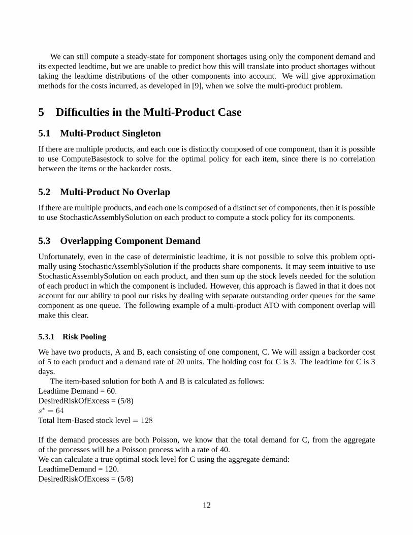
5.3.1 Risk Pooling

We have two products, A and B, each consisting of one component, C. We will assign a backorder costof 5 to each product and a demand rate of 20 units. The holding cost for C is 3. The leadtime for C is 3days.

The item-based solution for both A and B is calculated as follows:Leadtime Demand = 60.DesiredRiskOfExcess = (5/8)s∗ = 64Total Item-Based stock level= 128

If the demand processes are both Poisson, we know that the total demand for C, from the aggregateof the processes will be a Poisson process with a rate of 40.We can calculate a true optimal stock level for C using the aggregate demand:LeadtimeDemand = 120.DesiredRiskOfExcess = (5/8)

12

s∗ = 126The Product-Based policy overestimates the risk of stocking out and will accumulate excess holdingcosts.

5.3.2 Backorders and The Joint Cost Function

The ’Risk Pooling’ example suggests that to calculate the optimal policy for each component based onindependent item calculations, we should calculate for the aggregate component demand stream, ratherthan solving a single-item problem for each product and extending the solution to its components. How-ever, this approach makes it difficult to assess the shortage costs for each item, as the exact shortage costfor a unit of each component must consider the penalties that could result from a shortage of each productthe component is in, and in the correct proportions. In the assembly system approach, we recognized thatwhen we underorder for one component, we incur penalties not only for failure to fill demand on time,but for the excess of other components that we now hold. The extent of these penalties is dependent onthe joint stock policy. We will now look at how the optimal vectors can be calculated.

We can use the queuing approach to aid in developing an expression for the expected cost. If we havesteady-state values for theI(s) andB(s), then we can use them to calculate expected costs [9]. For anycomponent, the total expected costs will have a holding cost component and a penalty cost component.The holding cost component will be dependent onI(s) and onhi. The penalty cost component will bedependent onB(s) and on bothhi andbj, since component shortages result in both product shortagesand excess inventory of other components.

As in the derivation of the optimal basestock policy, the cost function will consist of steady-stateinventory,

∫ si0 (si − Xi) dxi. = [si − Xi]

+ times the cost of overordering, and steady-state backorders∫∞si

(X−si) dxi. = [Xi − si]+ times the cost of underordering.bj is a shortage cost applied to products,

and we will thus have to assess a penalty ofbj on product shortages, which have a steady-state rate ofBK(s). One component of the cost function will be this product

∑j bjE[Bj(s)]. hi is a unit holding

cost applied to components. It is clear that we will incur a costhi ∗ [si −Xi]+ which by the steady state

identities is equivalent to[si −Xi + Bi(si)]. This cost covers the holding cost for holding inventory upto our basestock levels.

Still missing from our cost function is a term to represent the holding costs incurred on comple-mentary components when a component is backordered. Sincehi is a per component cost, this must becomponent-based. The rate at which we experience shortage related holding costs for componenti isJi(s) =

∑j3i[B

j(s)−Bji (si)]. [Bj(s)−Bj

i (si)] is the difference in that rate of backorders for productjand the rate of shortages for componenti resulting from demand forj. This difference represents the rateat which componenti is delivered to meet demand forj, only to be held because of a shortage of anothercomponent.[9] shows that the expected costs sum to:

C(s) =∑

i hisi +∑

j b̃jE[Bj(s)]

whereb̃j = bj +∑

iεj hi

The backorder cost for one component is dependent on the backorder rate of other components and thustheir policies, making the overall backorder cost minimization problem a non-separable function of thejoint distribution.

The approach outlined in [9] is to solve an independent problem for each component to determine itsoptimal level. We estimate the shortage costs that a backorder of componenti will cause in each productj, iεj in such a way that we are assured an upper bound on each components basestock level. This

13

eliminates the problem of not having an accurate way of translating product demand into componentdemand (because of risk pooling) or component costs into product costs(due to an inseparable functionfor backorder costs). However, the approach is difficult to implement in that it involves evaluatingC(s),which is a difficult problem in itself.

We experiment with evaluatingC(s) through simulation. The benefits of this approach are limitedby the problem that inexact cost values can disrupt the convexity ofC(s) and the time required to reachsteady state average costs makes the algorithm undesirable for practical use.

6 Approximations

6.1 Upper Bound

In the equation for the optimal cost, the total backorder cost is calculated for products, and is a functionof the product backorder rate and the product backorder cost. In order to separate the cost equation, abound can be put on the effect that a change in one items basestock has on the total backorder costs.Recall thatBj(s) = maxiεj Bj

i (si)An effect of this is that:Bj(s + ei)−Bj(s) ≥ Bj(s). [9]We expect the derivative of the function of Steady-State backorders due to type j demand from item i torelate to that of all demand for item by the ratioλj

λi, the ratio of demand for productj, to that of itemi.

(Note that if we relax the unit matrix restraint we need to multiply this byaji.)Thus, if we take the expectation of the above inequality, we get the relationship we need between the

derivatives:4iBj(s) ≥ 4iB

Ki jsi) = λj

λi4Bi(si)

Since the derivative of the holding costs is constant with respect tos, this inequality containing thederivative of the backorder costs can be extended to the derivative ofC(s). From this we can obtain that4iC(s) ≥ 4iCI(s). [9] show that by the submodularity of C(s), this leads directly to the conclusion thats∗i ≤ sI∗

i for all i. Thus, if we optimizesi for bi =∑

j3iλj

λi(bj +

∑jεj

hj) we obtain a lower bound ons∗.Essentially, we have shown that by overstating the effects of a component shortage, we can achieve a

definite upper bound ons∗. The unit backorder cost is determined by two things. When components over-lap products, the difficulty is to assess what portion of the backorders for a component will be expressedby a late order in each product. Furthermore, when a backorder for componenti causes a penalty on anorder of productj, what is the additional cost that can be expected because of holding costs paid on othercomponents in that product that have already arrived at the supplier. These expectations are calculatedby integrating over an exponential number of permutations of leadtime distributions [8], but we can onlyestimate when deriving closed form approximations [9]. The cost calculation associated with the aboveupper bound forsi assumes that every time a component is backordered, it causes a penalty that wouldnot have already been caused by a shortage of a complementary component.

Thus, for each component, when we compute the upper bound, we assume that:

1. The unit shortage cost for componenti includes a portion of costs from each product,j, that isproportional to the expected costs of a shortage of productj caused by a backorder of componenti, by the proportion of demand for componenti that comes from productj.This means that we expect a shortage penalty to result from every backorder of producti, (

∑j3i

λj

λi=

1), and that any shortage ofK that occurs when multiple components are out of stock, is counted

14

multiple times.

2. Each time there is a backorder of componenti resulting in a shortage of productj, we expect toincur as a result of that backorder of componenti, a holding cost on every item inj other thani.

The above provides an intuitive description to accompany the mathematical proof of [9]. This typeof understanding is necessary in looking for a lower bound to increase the effectiveness of the closedform approximations. [9] provide no mathematical proof for their suggested lower bound, but pointto extensive empirical evidence. The goal in determining a lower bound would be to understate theeffects of a shortage, rather than overstate. The counterpart of our upper bound would be to assumethat all of the components that are packaged in a product with componenti are stocked out whencomponenti is stocked out. This estimate is both unrealistic and too low to be effective. A tighterlower bound is suggested by [9], with justification provided in that paper. We computed this bound:pi = Σj={i}

λj

λi + Σj3i,j 6={i}λj

2maxcεj{λc}(pj +

∑cεj,c 6=i hc)

This bound is based on the idea that if the shortages of respective components in a product occur si-multaneously as much as possible, the product backorder rate will be the maximum of all componentsbackorder rates, since no other component will cause a product shortage when this components is instock.The two bounds described in this section yield the following algorithms, used to initiate our search pro-cedures:

ComputeUpperBoundinputs:ATO Systemoutput:m-vector,s, of Upper Bounds on Optimal Basestock levels

1. ∀i

2. λi = Σj3i aji ∗ λj

3. pi = Σj3iλj

λi(pj +

∑cεj,c 6=i hc)

4. ∀i

5. si = ComputeStochasticBasestock(λi, li, pi, hi)

ComputeLowerBoundinputs:ATO Systemoutput:m-vector,s, of Lower Bounds on Optimal Basestock levels

1. ∀i

2. λi = Σj3i aji ∗ λj

15

3. pi = Σj={i}λj

λi + Σj3i,j 6={i}λj

2maxcεj{λc}(pj +

∑cεj,c 6=i hc)

4. ∀i

5. si = ComputeStochasticBasestock(λi, li, pi, hi)

7 Search Algorithms

We implement search algorithms to obtain solutions better than those given by closed-form approxima-tions. [9] suggest that the a global optimal solution can be reached in polynomial time using a SteepestDescent or Best Improvement method. This claim, however, rested on the ability to evaluate the costfunctionC(s) exactly. They rely on existing methods for minimization of submodular functions to findthe best neighbor policy. The simulation-based Best Improvement search relies on an exponential num-ber of simulations to find the minimum of the neighborhood that they suggest, and is thus impractical,despite its it optimal performance. We use the same methods in generating bounds to the optimal policybut use simulation-based comparisons and experiment with search algorithms that will be more practicalthan Best Improvement.

This section will describe the general structure of the algorithm we use to find a basestock, and sev-eral searches that we have implemented and tested.

Algorithm: FindCorrelatedPolicyInputs: ATO System, StartingBound, SearchType, SimDaysOutputs: Vectors of component basestock levelsInitialize:UpperBound← ComputeUpperBound(ATO)LowerBound← ComputeLowerBound(ATO)s← StartingBounds′ ← s

1. while (s′ = s)

2. s′ ← s

3. s←Search(ATO system,s, SimDays)

4. Returns

To initialize, we call the ComputeUpperBound and ComputeLowerBound algorithms from above. Weexperiment by altering the search used in step 3. The “Steepest Descent” search was implemented asfollows:

Best Improvement SearchInputs: ATO System,s, SimDaysOutput: s∗

Initialize:s∗ ← sH ← {s′ | ∀i, (si − s′i)ε{0, 1}}

16

1. ∀s′εH

2. if Evaluate(s′, ATO, SimDays) < Evaluate(s∗, ATO, SimDays)

3. s∗ ← s′

4. returns∗

To reduce search time, we replaced Best Improvement Search with First Improvement Search, or “Hill-Climbing”:

First Improvement SearchInputs: ATO System,s, SimDaysOutput: s∗

Initialize:s∗ ← sH ← {s′st.‖(si − s′i)‖ = 1, iε{1 . . . m} ∧ si = s′i, h 6= i}

1. while(s∗ = s ∧H 6= ∅)

2. randomly chooses′εH

3. H ← H − s′

4. if Evaluate(s′, ATO, SimDays) < Evaluate(s∗, ATO, SimDays)

5. s∗ ← s′

6. returns∗

Since First-Improvement finds a local minimum (as does steepest descent, though with a greater prob-ability that the local will also be a global minimum, in our case), the initialization is important. Typically,the search can be executed multiple times, with random restart positions used. We tried starting it twice,using each bound as a starting position. Finally, we improved on the performance of First Improvementby implementing Simulated Annealing:

Simulated AnnealingInputs: ATO System,s, SimDays, Cooling ScheduleOutput: s∗

Initialize:s∗ ← ss′ ← s H ← {s′st.‖(si − s′i)‖ = 1, iε{1 . . . m} ∧ si = s′i, h 6= i}T according to Cooling Schedule

1. while(s∗ = s ∧H 6= ∅)

2. randomly chooses′′εH

3. H ← H − s′′

17

4. 4(s′, s′′)← Evaluate(s′′,ATO,SimDays) - Evaluate(s′,ATO,SimDays)

5. if rand[0, 1] ≤ exp{−4(s′,s′′)T}

6. if Evaluate(s′′, ATO, SimDays) < Evaluate(s∗, ATO, SimDays)

7. s∗ ← s′′

8. Update T according to schedule

9. returns∗

For a cooling schedule we obtained good results by initializingT = 4, and cooling according to thescheduleTi = 4 ∗ .8

i2 , wherei is the total number of search iterations that have been executed. Each

iteration consists of a full execution of the algorithm above, which itself is called iteratively from Find-CorrelatedPolicy. All of these searches are iterative and generate a new neighborhood for their solutionuntil a local a minimum is found, though this part of the search has been abstracted into the FindCorre-latedPolicy algorithm in this section.

8 Simulation

Our search is dependent on our ability (imperfect as it may be) to evaluate the level of costs that weexpect to incur when implementing a particular basestock policy, and thus to choose the better of two ormore policies. We do this by simulation, using our own ATO simulator. We simulate both the behaviorof the market, through randomly generated demands and leadtimes, and the behavior of our agent, bymanaging inventory with an Order-Up-To mechanism.The design of the simulator is as follows:

ATO SimulatorInput: ATO, Simulation Length, PolicyOutput: Cost/Day

• The product structure of the ATO is expressed as ann ×m matrix A, whereaij is the number ofunits of componentsi needed to assemble one unit of productj.

• For each product, there is a sale price and a demand distribution associated with it.

• Each day’s demand is generated by samplingn Poisson demand distributions.

• For each component, there is a cost of purchase and a leadtime distribution associated with it.

• Leadtime is discretely distributed, with an expected delivery date, and probabilities associated toa finite number of delay lengths. A component’s leadtime distribution is randomly sampled everytime an order is placed for the component, to determine when that components will arrive (thisinformation is stored internally in the order and only the distribution is known to the agent).

A high-level view of a simulation day is as follows:

18

1. Supplier Progress: All orders due are moved one day closer to arrival. Orders that have reachedtheir arrival date are removed from the outstanding orders queue and added to the stock of physicalinventory. When a component arrives, its cost is subtracted from the starting balance.

2. Daily Demand: All of the product demand distributions are sampled, and the matrixA is usedto convertdj(t) into dj(t) ∗ A = di(t). Component demands are then added into the queue ofbackorders waiting to be filled. Existing backorders and the newly generated demand are filleduntil supply runs out, at which point, a late penalty is assessed for all items remaining in thebackorder queue. When an item is filled, its sale price is added to the balance.

3. Restock: Orders are placed for components according to the policy that was input at the start of thesimulation. Specifically, for each componenti, zi = s− yi + wi − xi is ordered, and that quantityis added to the queue of orders due from the supplier. A leadtime, sampled from the distribution isassigned to each order.

4. End of Day: A holding penalty is subtracted from the balance for each unit of stock that remainsin physical inventory at the end of the day. In TAC, interest will be accumulated at this time, withholding costs coming in the form of lost interest.

Since we are trying to minimize computation time, we want to keep our simulations as short as pos-sible. However, a large number of cycles are required for convergence to steady-state values and thusfor accurate cost predictions. Still, the policy that performs better in a short simulation is likely, withsome likely probability, to perform better in the steady-state. Part of our research has been directed atdetermining a simulation length that will evaluate correctly with a large probability while using only aminimum of computation time. The table below shows the average distance form the mean in samplesof cost estimates taken at different lengths in an ATO system that we studied. The variance continues toreduce dramatically as the simulation length is extended up to 20,000 days of simulation, but stabilizesthereafter. Thus, we accept the results of 25,000 day simulations as steady-state results and base on outperformance evaluations on these figures. Simulations performed while searching must be considerablyshorter, with a goal of simulating less than 100 days. The table shows a good deal of variance in the costestimates at this length. There is enough variance that the policy chosen through a comparison based ondata obtained at this length will not necessarily be the better policy with steady-state data. The effects ofthis error on the performance of policies obtained through search are examined in the Results section.

Simulations Days Avg Distance from Mean in 10 samples5000 4.215259999999989

10000 4.26007199999996815000 3.84468000000000520000 3.798437333333322625000 1.926336000000037630000 1.79210000455

Figures 2-4 in the appendix show data collected from simulations of a two-product system with cor-relation. Multiple polices were simulated in an attempt to characterize the cost function for the system.

• Figure 2 shows data collected from 25,000 day simulations with policy increments of 5 to show thegeneral convexity of the cost function.

19

• Figure 3 shows data collected from 25,000 day simulation with policy increments of 1. The curveis not smooth, because their is correlation, but there is only a global minimum.

• Figure 4 shows data collected from 15,000 day simulations, and stochastic leadtimes (Figure 2 useddeterministic, which speeds convergence). The curve has a similar general shape, but local minimaexist. Actual searches will have more variance than in figure 4.

9 Results

The following is a summary of results we obtained in testing of search algorithms on a number of twoand three-product ATO’s. We tested over a range of simulation lengths (for evaluation) and cost ratios.Refer to the appendix for more specifics. For consistency, we present data collected, except when it isstated that we are testing a range of a particular variable, from the following three-product ATO, whichwe will call the “Test System”.

ATO: TestSystemComponents: A,B,C∀i, ϕ(li) :

• 3 days: 50%

• 4 days: 30%

• 5 days: 20%

Each component has a cost of$10 per unit.Holding costswere identical for each components but varied among simulations.Products: A,B,ABC

• Product A:$50 per unit,pA = 30, Poisson Demandλ = 3

• Product B:$90 per unit,pB = 54, Poisson Demandλ = 6

• Product ABC:$90 per unit,pABC = 54, Poisson Demandλ = 6

9.1 Closed-Form Performance

One of the most important results we obtained was that the bounds proposed by [9] worked well inpractice. In experiments conducted on two and three product systems with correlated demands, weconsistently found the optimal to lie between these bounds. Moreover, the bounds were sufficiently tightto suggest that they may be of use as approximations in environments where decision time is severelylimited; TAC being among these situations.

Though tests on larger systems are still necessary, these results are encouraging. In comparison of theperformance results of the upper bound policy to those of the optimal policy, we consistently found thecosts/day to be within 5% of the optimal in 25000 day simulations.

20

9.2 Computation Time

Using the upper bound as a policy would have obvious advantages in terms of computation time, asno search is necessary. Even among searches, there was a significant range of search times. Since thelimiting factor in the speed of a search is the number of simulations that are needed before terminationof the algorithm, we compared computation time by keeping track of the average number of simulationsneeded by each algorithm as an indicator.

Search procedures were tested on the Test System, with a range of simulation lengths. Below areaverage number of simulations per search for 200 searches spread uniformly over the range of simulationlengths{10, 20, . . . , 100}

• Steepest Descent: 22.2 sims

• First Improvement: 6.2 sims

• First Improvement w/ restart: 11.4 sims

Clearly, there is a computational advantage for either First-Improvement algorithm in comparison toSteepest Descent. Since Steepest Descent must evaluate every policy in its neighborhood, the number ofsimulations it requires makes it unattractive for use in a TAC environment. Finally, the advantage gainedby First Improvement was so drastic, that restarts could be used while maintaining an improved searchtime. This improved performance over the single First Improvement considerably.

9.3 Search Performance

The improved search time of the First-Improvement search did not come without a tradeoff in perfor-mance. Both Steepest Descent and First Improvement find global optimum policies given perfect evalua-tion, and both fell short of this mark when using simulation data. First Improvement, however, followingan often more convoluted path to the optimal, was more susceptible to errant evaluations. Thus, theSteepest Descent begins consistently near-optimal behavior at much shorter simulation lengths than FirstImprovement. (See Figure 5)

This affect carried through into the shortest simulation lengths, where Steepest Descent outperformedFirst Improvement in all but those cases where the optimal was extremely close to one of the bounds.However, First Improvement w/ Restart and Simulated Annealing performed significantly better, chal-lenging the average performance of Steepest Descent in considerably less time.

9.4 Conditions

Since the performance of First Improvement was overly sensitive to starting position, “Restarts” seem tobe a necessary extension. By searching from both bounds, First Improvement w/ Restart was less affectedby changes in the cost ratio, whereas First Improvement search from the upper or the lower performedwell only under certain conditions (compare performance of “firstupper” and “firstlower” in Figure 7and Figure 8). Steepest Descent also proved to be relatively robust. Results are given for a range ofholding costs (with penalty cost held constants) to gauge the effect that the cost ratio had on each policy’seffectiveness.

21

9.5 Conclusion

Other than Steepest Descent, all of the algorithms seem to be heavily affect by the starting location atlow simulation lengths. Still, the time saved is enough that several restarts can be executed in the timeof a single Steepest Descent algorithm. It is clear, that in the case of small simulation lengths, a globalminimum is far from assured. Under these conditions, a greedy algorithm is likely not to be the bestmethod since it cannot recover from a mistake made as as result of error in evaluation. This explains theperformance gains made by Simulated Annealing relative to First Improvement. Unfortunately, (froman efficiency viewpoint), the more evaluations that are made, the lower the probability is that the overallperformance will be significantly affected by errant values. This would suggest that it is worth the timeto try a longer search. However, the accuracy of our closed form approximations, and perhaps our abilityto add further heuristics about the policy to which we should initialize, make it fairly certain that usingmultiple randomized searches, that are likely to terminate quickly, will turn out a good result.(See Figure6)

10 Future Work

10.1 Heuristics

The success of closed form approximations suggests that it will be possible to perform reasonably wellwithout spending any time searching. The experiments showed that higher ratios of holding to shortagecosts yielded optimal policies closer to the lower bound,and lower ratios yielded policies nearer the upperbound. A future problem will be to determine a heuristic strategy that bids the upper or lower bounddepending on some type of average cost ratio. Preliminary results using the average of upper and lowerbounds, as well as a weighted average toward the (generally) tighter upper bound have been promising.

10.2 Leadtime Correlation

Demand correlation is a difficult problem for which some background exists, but leadtime correlationis a very much untouched topic. We are attracted to this problem (of correlation across time periods)because of closeness to real life situations, where a supplier delay in one time period is likely to indicatea shortage that could “ripple” into future periods. This problem is difficult in that it violates many of thekey assumptions of our model, namely the applicability of a queuing system, which ensures steady-stateconvergence in the model that we have been using.

10.3 Leadtime Decisions

Another way in which the leadtime could be more accurately modeled is by changing leadtime to anendogenous variable, taking only cost/leadtime tradeoffs as exogenous. This is representative of the TACenvironment, as well as real life situations to which SCM agents may be applied.

22

[1.]Kenneth Arrow, Samuel Karlin, and Herbert Scarf. “Studies in the Mathematical Theory ofInventory and Production” California: Stanford University Press (1958)

[2.]Guillermo Gallego, "Material Requirements Planning (MRP) - IEOR 4000 - Production Man-agement"Citeseer url: citeseer.nj.nec.com/493501.html

[3.]Hillier and Lieberman, “Introduction to Operations Research”, 7th edition, New York:McGraw-Hill Textbook form AM120

[4.]H. Van Dyke Parunak, Robert Savit, Rick L. Riolo, Steven J. Clark, “DASCh: Dynamic Anal-ysis of Supply Chains” (1997)Citeseer url: citeseer.nj.nec.com/parunak99dasch.html

[5.]Fikri Karaesmen, Yves Dallery “A Performance Comparison Of Pull Type Control Mecha-nisms For Multi-Stage Manufacturing” (1998)Citeseer url:citeseer.nj.nec.com/karaesmen98performance.html

[6.]Fikri Karaesmen, John A. Buzacott , “Integrating Advance Information In Pull Type ControlMechanisms For Multi-Stage Production”Citeseer url : citeseer.nj.nec.com/204724.html

[7.]Lee YH, Kim SH. “Optimal Production-Distribution Planning in Supply Chain Managementusing a hybrid Simulation-Analytic Approach” (2000)url: http://www.informs-cs.org/wsc00papers/169.PDF

[8.]Yingdong Lu, Jing-Sheng Song, David D. Yao “Order Fill Rate, Leadtime Variability, andAdvance Demand Information in an Assemble-to-Order System” (2001)Citeseer url: citeseer.nj.nec.com/484612.html

[9.]Yingdong Lu, Jing-Sheng Song, David D. Yao "Order-Based Cost Optimization in Assemble-to-Order Systems". (2002)

[10.]Murota, Kazuo. "L-Convex Functions And M-Convex Functions". (1998)Citeseer url = citeseer.nj.nec.com/murota98lconvex.html

[11.]Murota, Kazuo. "Algorithms in Discrete Convex Analysis". TIEICE: IEICE Transactions onCommunications/Electronics/Information and Systems (2000)Citeseer url = citeseer.nj.nec.com/murota00algorithms.html

[12.]Jing-Sheng Song, Paul Zipkin, "Assemble-to-Order Systems". Chapter 13 inHandbooks inOperations Research and Management Science, VOl. XXX: SupplyChainManagement. T.de KoKand S.Grave(eds.). North: Hollandurl = http://www.gsm.uci.edu/ song/Working%20Paper/Atocto03Nov02.pdf

11

[13.]Viswanadham Srinivasa, "Lead Time Models for Analysis of Supply Chain Networks"Citeseer url : citeseer.nj.nec.com/208334.html

[14.]Ramesh Srinivasan, Rangarajan Jayaraman, James A. Rappold, Robin O. Roundy, SridharTayur “Procurement of Common Components in a Stochastic Environment” (1998)Citeseer url : "citeseer.nj.nec.com/srinivasan98procurement.html"

[15.]Sridhar Tayur “Computing Optimal Stock Levels for Common Components in an AssemblySystem” (1995)Citeseer url =:‘citeseer.nj.nec.com/159591.html’

[16.]Daniel Dajun Zeng, Katia Sycara. “Dynamic Supply Chain Structuring for Electronic Com-merce Among Agents” (1999)Citeseer url : citeseer.nj.nec.com/zeng99dynamic.html

[17.]Wagner, HM, and TM Whitin, “Dynamic Version of the Economic Lot Size Model”Management Science, Volume 5, Issue 1 (Oct. 1958), 89-96

12

0

50

100

150

200

250

300

350

400

40 45 50 55 60 65 70 75 80

Dai

ly A

vera

ge($

)

Policy(Items)

Figure 1: Single-Item Example (Section 3.3.1)

totalcostslatepenalties

holdingpenalties

220 240 260 280 300 320 340 360 380 400 420

40 45 50 55 60 65 70 75 80

Dai

ly A

vera

ge($

)

Policy(Items)

Figure 1: Single-Item Example (Section 3.3.1)

revenuetotalcosts

Figure 2: Cost/Day A:20, AB:20

150 155 160 165 170 175 180 185 190 195 200Policy A 60

65 70

75 80

85 90

95 100

Policy B

700 800 900

1000 1100 1200 1300 1400 1500 1600 1700

Cost/Day

Figure 3: Cost/Day A:20, AB:20 detLT

132 133

134 135

136 137

138Policy A 64

65 66

67 68

69 70

71 72

73

Policy B

765 770 775 780 785 790 795 800 805 810 815

Cost/Day

Figure 4: Cost/Day A:20, AB:20

161 162

163 164

165 166

167Policy A 79

80 81

82 83

84 85

86 87

Policy B

785 790 795 800 805 810 815 820 825 830

Cost/Day

630

635

640

645

650

655

660

665

0 200 400 600 800 1000 1200 1400 1600

Cos

t/Day

s w

ith S

olut

ion

Simulation Days per Cost Evaluation

Figure 5: Performance of Longer Searches in 3-product setting with h = 20

First ImprovementSteepest Descent

400

500

600

700

800

900

1000

1100

0 10 20 30 40

Cos

t/Day

s w

ith S

olut

ion

holding cost

Figure 6: Effects of Cost Ratio on Performance

Steepest DescentFirst Improvement

First w/RestartSimulated Annealing

685

690

695

700

705

710

715

10 20 30 40 50 60 70 80 90 100

Cos

t/Day

s w

ith S

olut

ion

Simulation Days per Cost Evaluation

Figure 7: Performance of Search Solutions for three product ATO, h = 20

steepestfirstupperfirstlowertwostartsSAupperSAlower

428

429

430

431

432

433

434

10 20 30 40 50 60 70 80 90 100

Cos

t/Day

s w

ith S

olut

ion

Simulation Days per Cost Evaluation

Figure 8: Performance of Search Solutions for three product ATO, h = 5

steepestfirstupperfirstlowertwostartsSAupperSAlower