Chemometrics and Intelligent Laboratory Systems 126 (2013) 108–116
Contents lists available at SciVerse ScienceDirect
Chemometrics and Intelligent Laboratory Systems
j ourna l homepage: www.e lsev ie r .com/ locate /chemolab
Optimization of the multianalyte determination with biasedbiosensor response
Romas Baronas a,⁎, Juozas Kulys b, Antanas Žilinskas c, Algirdas Lančinskas c, Darius Baronas c
a Faculty of Mathematics and Informatics, Vilnius University, Naugarduko 24, LT-03225 Vilnius, Lithuaniab Institute of Biochemistry, Vilnius University, Mokslininku 12, Vilnius LT-08662, Lithuaniac Institute of Mathematics and Informatics, Vilnius University, Akademijos 4, LT-08663 Vilnius, Lithuania
The investigation is dedicated to the optimization of calculation of multianalyte concentrations using a responseof a biocatalytical amperometric biosensor. Mathematical and corresponding numerical models for a single en-zyme two substrates amperometric biosensor were built to generate pseudo-experimental responses to mix-tures of compounds. Numerically simulated biosensor responses to different concentrations of the substrateshave been used to extract the information on the dependence of the transient output signal on the concentra-tions of the compounds. The resulting information has been used to construct a mathematical optimizationmodel for determination of the concentrations of the compounds from a given transient biosensor response. Anumerical implementation of the optimization model has been used to investigate opportunities and the preci-sion of the determination of different concentrations. The influence of the possible discrepancy of the measure-ments of biosensor response, such as different types of trend orwhite noise, to the precision of the determinationhas been also investigated. The numerical experiments showed that the precision of the concentrations estima-tion significantly depends on the biosensor response being under either the diffusion or the enzymekinetics con-trol. The concentration estimation is more accurate for a substrate corresponding to a greater diffusion modulethan for another substrate corresponding to a lower diffusion module.
The signal (response) of biosensors is generated in the presence ofa substance (an analyte) that is of interest in an analytical procedure[1,2]. The calculation of analyte concentration, i.e. “reverse problemsolving” is simple in the case of a linear dependence of the biosensorresponse on the substance concentration (linear calibration) [3,4].The problem becomes more complex in the case of nonlinear calibra-tion or in the presence of mixtures of substances producing the bio-sensors response [5–7]. The task becomes even more complex if thebiosensor response is perturbed by noise, e.g. white noise, sinusoidalpower electrical noise, or if the biosensor response is biased, e.g. bytemperature change [8–10].
The multivariate calibration using partial least squares has beenalready successfully applied for quantitative analysis of binarymixtures by dual amperometric biosensor [11]. Four different chemi-thermo-mechanical pulpwastewater sampleswere clearly discriminat-ed using an array of eight amperometric biosensors in a combinationwith principal component analysis [12]. Multi-component mixtureshave been also analyzed using a combination of an amperometric
s).
rights reserved.
biosensor with artificial neural networks [13–16]. In those analyticalsystems several enzymes or even several enzyme electrodes wereused. More complexmethods and tools are needed to handle and inter-pret the information obtained in the systemswheremultiple substratesreact with a single enzyme.
Optimization methods have been also successfully applied to theanalysis of the biosensor responses. The relaxation, simplex, Taguchiand someother algorithms have been used to study the electrochemicalresponses, mainly in order to optimize the parameters of analytical sys-tems [17–22]. Recently, an optimization-based approach was intro-duced to quantification of mixtures by multiple enzymes assumingnoise-free signal measurements [23]. The trend and noise or back-ground current typically bring about a level of uncertainty in the system[8,9,22,24,25].
To the best of our knowledge the analysis of the problem of analytesdetermination by reverse problem solving has not been explicitly for-mulated though the optimization of the biosensors response has beenperformed in many publications [17–21].
The task of our investigation is to optimize the calculation ofmultianalyte concentration using a response of a biocatalytical ampero-metric biosensor [1,2]. The basis of multianalyte determination ismultisubstance (nonspecific) enzyme-catalyzed substances conversion[26,27]. The influence of white noise as well as temperature inducedtrend to the calculation of the analytes concentrationwas also analyzed.
109R. Baronas et al. / Chemometrics and Intelligent Laboratory Systems 126 (2013) 108–116
Mathematical and corresponding numerical models for a single en-zyme two substrates amperometric biosensor were built to generatepseudo-experimental responses tomixtures of compounds. Numerical-ly simulated biosensor responses to different concentrations of thecompounds were employed to extract the information on the depen-dence of the transient output signal on the compounds concentrations.The resulting information was then used to determine the concentra-tions of the substrates from the testing simulated measurements.
Themathematicalmodel of the biosensor is based on non-stationaryreaction–diffusion equations [28]. The model comprises a layer of anenzyme entrapped on the electrode surface. The computational simula-tion was carried out using the finite difference technique [28–30]. As-suming good enough adequacy of the mathematical model to thephysical phenomena, the simulated biosensor responses were used in-stead of experimental data. The computer simulation is usually muchcheaper and faster than real experiments. The simulation is especiallyreasonable when the practical sensors are under development. Thenthe development of intelligent analytical systems and their optimiza-tion may be carried out in parallel [18,19,25,31–33].
2. Mathematical model
We consider a mono-enzyme multi-biosensor (many substrates)utilizing the Michaelis–Menten kinetics [1,2,26],
Eþ Sik1i⇌ESi→
k2 i Eþ Pi; i ¼ 1;…; k; ð1Þ
where E denotes the enzyme, Si is the substrate, ESi stands for the en-zyme and substrate complex, Pi is the reaction product, kinetic con-stants k1i , k−1i and k2i correspond to the respective reactions: theenzyme substrate interaction, the reverse enzyme substrate decom-position and the product formation, and k is the number of substratesto be analyzed.
When substrates S1, …, Sk (k > 1) react with a single enzyme Ewithout formation of any multi-fold complex containing two or moresubstrates, and the substrates do not combine directly with eachother, then in mixtures of S1,…, Sk each substrate acts as a competitiveinhibitor of the others [34,35].
The biosensor to be modeled is intended to analyze a mixture of ksubstrates (compounds). Practical mono-enzyme analytical systems areusually limited to determining only a few (often to two) substrates [26].
The reactions in the network (1) are usually of different rates[2,34]. The large difference of timescales in the reactions creates dif-ficulties for simulating the temporal evolution of the network and forunderstanding the basic principles of the biosensor operation. Tosidestep these problems, the quasi-steady-state approach (QSSA) isoften applied [36,37]. According to the QSSA, the concentration ofthe intermediate complex does not change on the time-scale of prod-uct formation.
The amperometric biosensor is treated as an electrode and a rel-atively thin layer of an enzyme (enzyme membrane) applied ontothe probe surface. The biosensor model involves two regions: theenzyme layer where the biochemical reactions (1) as well as themass transport by diffusion take place, and a convective regionwhere the concentrations of the substrates are maintained con-stant. Assuming a symmetrical geometry of the electrode and a ho-mogeneous distribution of the immobilized enzyme in the enzymelayer of a uniform thickness, the mathematical model of the bio-sensor action can be defined in a one-dimensional-in-space domain[30,38].
2.1. Governing equations
Applying QSSA and coupling the enzyme-catalyzed reactions (1)in the enzyme layer with the one-dimensional-in-space diffusion,
described by Fick's law, lead to the following system of equations ofthe reaction–diffusion type (t > 0):
∂Si∂t ¼ DSi
∂2Si∂x2
−Vmaxi
Si
KMi1þ∑k
j¼1Sj=KMj
� � ;
∂Pi
∂t ¼ DPi
∂2Pi
∂x2þ Vmaxi
Si
KMi1þ∑k
j¼1Sj=KMj
� � ; i ¼ 1;…; k;0 b x b d;ð2Þ
where x and t stand for space and time, respectively, Si(x,t) and Pi(x,t)correspond to the molar concentrations of the substrate Si and theproduct Pi, respectively, Vmaxi
is the maximal enzymatic rate attain-able with that amount of the enzyme when the enzyme is fully satu-rated with the substrate Si, KMi
is the Michaelis constant, d is thethickness of enzyme layer, DSi
and DPiare the diffusion coefficients,
Vmaxi¼ k2i E0, KMi
¼ k−1i þ k2i
� �=k1i , and E0 is the total concentration
of the enzyme, i = 1, …,k.
2.2. Initial and boundary conditions
Let x = 0 represent the electrode surface, and x = d correspond tothe boundary between the enzyme layer and the bulk solution. The bio-sensor operation starts when all the substrates (S1,…,Sk) appear in thebulk solution (t = 0),
Si x;0ð Þ ¼ 0; Pi x;0ð Þ ¼ 0; 0≤ x b d;Si d;0ð Þ ¼ S0i ; Pi d;0ð Þ ¼ 0; i ¼ 1;…; k; ð3Þ
where S0i is the concentration of the substrate Si in the bulk solution,i = 1, …,k.
Due to the electrode polarization the concentrations of the reactionproducts (P1, …,Pk) at the electrode surface (x = 0) are permanentlyreduced to zero (t > 0) [38],
Pi 0; tð Þ ¼ 0; i ¼ 1;…; k : ð4Þ
Since the substrates are not ionized, the fluxes of their concentra-tions on the electrode surface were assumed to be zero (t > 0),
DSi
∂Si∂x
����x¼0
¼ 0; i ¼ 1;…; k : ð5Þ
The concentrations of the substrates and the products in the bulksolution remain constant during the biosensor operation,
Si d; tð Þ ¼ S0i ; Pi d; tð Þ ¼ 0; i ¼ 1;…; k : ð6Þ
3. Biosensor response
The biosensor current density I(t) at time t was expressed explic-itly from the Faraday and the Fick laws [34],
Ii tð Þ ¼ niFDPi
∂Pi
∂x
����x¼0
; i ¼ 1;…; k; ð7aÞ
I tð Þ ¼Xki¼1
Ii tð Þ; ð7bÞ
where Ii(t) is the density of the faradaic current generated by theelectrochemical reaction that involves oxidation or reduction of theproduct Pi, ni is the number of electrons involved in a charge transferat the electrode surface in the corresponding reaction, F is the Faradayconstant, F = 96,486 C/mol.
110 R. Baronas et al. / Chemometrics and Intelligent Laboratory Systems 126 (2013) 108–116
We assume that the system approaches a steady-state as t → ∞,
I∞ ¼ limt→∞
I tð Þ; ð8Þ
where I∞ is the density of the steady-state biosensor current.
4. Diffusion module
The diffusion module essentially compares the rate of the enzymereaction Vmaxi=KMi
� �with the mass transport through the enzyme
layer DSi=d2
� �[38,39],
Φ2i ¼ Vmaxi
d2
KMiDSi
; i ¼ 1;…; k; ð9Þ
whereΦi2 is the dimensionless diffusionmodule corresponding to i-th
reaction of the network (1).It is rather well known that if the diffusion module is less than unity
then enzyme kinetics (reaction rate) controls the biosensor response.The response is diffusion controlled or limitedwhen the diffusionmod-ule is greater than unity. At intermediate values of the diffusionmodulethe biosensor operation is of mixed control [40]. The diffusion module(9) is also known as the Damköhler number [38].
The quality of quantitative analysis of mixtures may notably de-pend on whether the biosensor response is under diffusion or enzymekinetics control [14,15].
5. Numerical simulation
Because of the nonlinearity of the governing Eq. (2) the initialboundary value problem (2)–(6) can be analytically solved only fora specific set of the model parameters [28,38].
The initial boundary value problem (2)–(6) was numericallysolved for the particular case of two substrates (dual biosensor,k = 2). The finite difference technique was applied for discretizationof the mathematical model [28–30]. A uniform discrete grid in bothdirections, space x and time t, was introduced to find a numerical so-lution. An explicit finite difference scheme has been built as a result ofthe difference approximation of Eqs. (2)–(6) [30,41]. The digital sim-ulator has been programmed in C++ language [42].
Explicit difference schemes are simple and have a convenient algo-rithm of the calculation and programming [28,30]. The calculation ofthe difference scheme was performed in the series one grid layer afteranother [41]. At first the solution on the zero layer at t = t0 = 0was cal-culated using the initial conditions (3). Further, having a finite differencesolution at layer t = tj the solution on the next layer t = tj + 1 = tj + τwas found, where τ is the time step size, j = 1, 2,…. To make the differ-ence scheme stable the time step size τwas found from the sufficient sta-bility conditions [30]. The size τ = 10−4 s was sufficient for allsimulations when dividing the enzyme layer into 200 points.
The mathematical as well as the corresponding computationalmodels of the biosensor were validated using known analytical solu-tions for mono-enzyme single substrate amperometric biosensors[30,38]. Those analytical solutions were derived for relatively low aswell as high concentrations of the substrates.
When the concentrations of the substrates are very small incomparison with the corresponding Michaelis constants ∀i∈ð1;…; kf g : S0i≪KMi Þ, the nonlinear reaction terms in Eq. (2) simplifyto those of the first order, Vmaxi=KMi
� �Si. Assuming this approximation
the nonlinear problem (2)–(6) reduces to a linear one, and the densityI∞ of the steady-state current can be expressed as follows [14,39]:
I∞ ¼ Fd
Xki¼1
niDSiS0i 1−1=cosh Φ2
i
� �� �: ð10Þ
For validating the model in the opposite case of very high substrateconcentrations, a high concentration S0i of the substrate Si(i = 1, …,k)was used together with zero concentrations of all other substrates,S0i≫KMi
and S0j ¼ 0;∀j∈ 1;…; i−1; iþ 1;…; kf g. At these conditionsthe nonlinear reaction terms reduce to those of the zero order (Vmaxi),and the density of the steady-state current I∞ can be calculated as follows[38]:
I∞ ¼ niFVmaxid=2: ð11Þ
The following values of the model parameters were kept constantin all the numerical experiments:
DSi¼ DPi
¼ 3� 10−10m2=s; ni ¼ 1; KMi
¼ 10−4M; i ¼ 1;2;
d ¼ 2� 10−4m:ð12Þ
The relative difference between the numerical and analytical solu-tions of the model (2)–(6) was less than 1% at different values ofVmaxiand S0i , i = 1,2.
6. Optimization problem
6.1. Statement of the optimization problem
We are interested in a method for estimating the concentrations ofsubstrates using the measurements of the faradaic current on a workingelectrode of an amperometric biosensor. The physico-chemical processesare supposed to be corresponding to the mathematical model describedby the Eqs. (2)–(7). That problem is an inverse problem with respect tothe problemof computation of the faradaic currentwhere the concentra-tions of the substrates are given. Similar problem for a simplermodel canbe successfully solved bymeans of an optimization-based approach [23].The optimization-based approach was introduced for quantification ofmixtures by multiple enzymes assuming noise-free signal measure-ments [23]. In the present paper we consider a significantly more com-plicated analytical system (1) where each substrate of the mixture actsas a competitive inhibitor of the others [26,34]. Moreover, here themea-surements are supposed to be corrupted by a random noise, and the re-action rate is supposed to be affected by the temperature variance [8,7].
The method developed is oriented to process experimental data.However, pseudo-experimental simulated data have been used for test-ing with reference to the proved adequacy of the mathematical model(2)–(7). The method was tested for a particular case of two substrates(dual biosensor, k = 2). Similar approach to using simulated biosensorresponse data was applied to training a neural network used to quanti-tative analysis of mixtures by a multi-enzyme system [14,15].
Let W = (w1, …,wn) be a sequence of measurements where theoutput of a biosensor (the faradaic current) has been measured atthe time moments t1, …,tn. The output of the biosensor simulatedaccording to the mathematical model (2)–(7) is denoted by z(t,c),where t is time, and c = (c1, …,ck)T denotes a vector of concentra-tions of the substrates S1, …,Sk, respectively.
The output values computed at the timemoments t1,…,tn constitutea vector denoted by Z(c) = (z(t1,c), …,z(tn,c))T. The concentrations ofthe substrates are supposed to be evaluated by tuning the theoreticaloutput of the biosensor to the corresponding measurements. The leastsquares approach is usually applied to tune the output data, computedaccording to a theoretical model, to the experimental measurements.This approach is especially appropriate for statistical data where mea-surements are corrupted by random noise. The least squares approachwhen applied to the solution of the stated above problem reduces tothe following minimization problem
~c ¼ argminc∈C
Xni¼1
z ti; cð Þ−wið Þ2; ð13Þ
111R. Baronas et al. / Chemometrics and Intelligent Laboratory Systems 126 (2013) 108–116
where C denotes the feasible region for the values of concentrations ofthe substrates.
The minimization problem (13) is relatively easy to solve in a casewhen z(t,c) is an affine function of x. However, in the considered herecase z(t,c) is a solution of a system of partial differential equations,and the desirable property of z(t,c) cannot be rigorously proved. In thecase of nonlinearity of z(t,c) with respect to c, the optimizationproblem (13) usually is difficult to solve because of the multimodalityof the objective function. Although various global optimizationmethods(see, e.g. [43]) theoretically can be applied to the solution of the consid-ered problem, practically the solution time frequently is unacceptablylong even for model functions defined by simple analytical formu-las [44,45]. In the considered case the additional difficulty of theproblem (13) is long computing time of z(t,c) (around 75 s usingIntel® Core™ i3 CPUM350, 2.27 GHz processor), and some imprecisionof the numerical solution of the Eqs. (2)–(7). A method to overcomethese difficulties is proposed in the next section.
In real applications the reaction rate can be affected by the tempera-ture change that causes a trend of the output of the considered sensor[8,46]. Let us describe the trend of the output as the multiplication ofthe initial output z(ti,c) by a factor R(ti), and assume that at the timemo-ment t0 = 0 the initial conditions are valid implying the equalityR(t0) = R(0) = 1. The trend factor R(t) can be expressed using theArrhenius equation which defines the dependency of the reaction rateon temperature R tð Þ ¼ Aexp −Ea= RT
� �� �, where A is the pre-exponential
factor, Ea is the activation energy,R ¼ 1:98 cal/(K mol)– the gas constant,and T is absolute temperature [20,47,48]. In calculations it was assumedthat temperature T is changing lineally with time, T(t) = T0 + at,where T0 equals 298 K, and a (K/s) is the coefficient of proportionality.
Calculating the pre-exponential factor A from the initial conditionR 0ð Þ ¼ 1 A ¼ exp Ea= RT0
� �� �� �leads to the following expression for the
factor R(t) of the exponential trend:
R tð Þ ¼ expEaR
� atT0 T0 þ atð Þ
� �: ð14Þ
Assuming the sensor output influenced by the Arrhenius trend, theconcentration evaluation problem should be reformulated as follows:
~c ~; að Þ ¼ arg minc∈C;a−≤a≤aþf g
Xni¼1
z ti; cð ÞR tið Þ−wið Þ2; ð15Þ
where the optimization variable a is the unknown parameter a in Eq.(14).
In some cases a linear trend is also of interest [8,47]. In the case ofthe linear signal trend, the optimization problem related to the eval-uation of concentrations can be described as follows:
~c ~;αð Þ ¼ arg minc∈C; α−≤α≤αþf g
Xni¼1
z ti; cð Þ þ αti−wið Þ2; ð16Þ
where the optimization variableα is interpreted as the rate of a lineartrend, and the feasible regions C and [α−,α+] are defined at due place.
In the all stated optimization problems data can be corrupted bynoise.
6.2. Solution of the optimization problem
The optimization problems stated are difficult because of the fol-lowing reasons:
• Neither convexity nor unimodality of the objective function ismathematically provable, and therefore applicability of local opti-mization algorithms here can be questionable,
• Long computing time is needed to compute a single value of the ob-jective function,
• Analytical gradients of the objective function are not available, andtheir numerical estimates can be strongly corrupted because of er-rors in numerical solution of the equations that describe the math-ematical model of the considered biosensor.
On the other hand, the considered optimization problem is of lowdi-mensionality, and it possibly can be solved by brute force methodsspending (allowably) much of computing time. However, some heuris-tically established properties of the considered optimization probleminduce an idea how to solve that optimization problemmore efficiently.
The function z(t,c), generally speaking, is not an affine function withrespect to concentrations c to be determined. However, practical bio-sensors are usually designed in such away that the steady-state currentz(t∞,c) would be linear in some intervals for the concentrations of thesubstrates to be quantitatively determined [1–3]. Therefore it can beexpected that transient responses z(t,c) deviate not too much from alinear function of concentrations c, implying unimodality of the statedabove optimization problems in an appropriate feasible region for c.One of the goals of the present research is to determine such a regionwhere a local optimization algorithmwould be acceptable for the solu-tion of the above-stated optimization problems.
To reduce the computation time of objective function values duringthe optimization process, the values of a surrogate function ~z t; cð Þ havebeen computed instead of the original values of the transient biosensorresponses z(t,c) simulated numerically or measured experimentally. Toensure the sufficient precision of such a replacement the function ~z t; cð Þis defined as a set of k-dimensional splines constructed for every ti usingthe values of z(t,c) obtained at various concentrations c1, …,ck of thesubstrates, i = 1, …,n.
Since at relatively low concentrations of the substrates (S0i≪KMi ,i = 1,…,k) the nonlinear governing equations describing the biosensoraction become linear, and therefore quantitative analysis of such mix-tures becomes rather easy [5,7,11], the proposedmethodwas evaluatedonly for moderate and relatively high concentrations of the substrates.
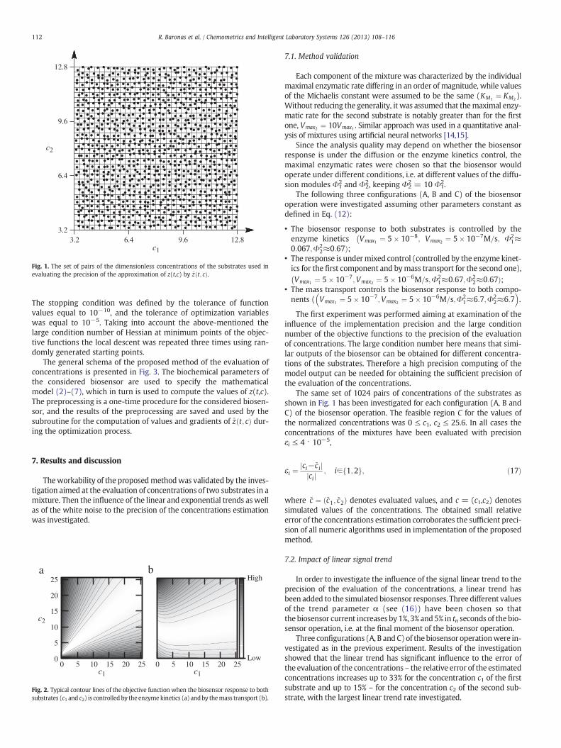
For a modeling dual biosensor (k = 2) specified in the previous sec-tion the reasonable intervals for concentrations of both substrates are3.2 ≤ c1, c2 ≤ 12.8, where c1 and c2 are assumed to be the dimensionless(normalized) concentrations, ci ¼ S0i=KMi , i = 1, 2. To derive the ap-proximation ~z t; cð Þ the entire quadratic domain [3.2,12.8]2 of the sub-strate concentrations was discretized with the uniform mesh step sizeof 0.3. The response of the model biosensor at its configuration parame-ters defined in Eq. (12) approaches the steady-state in about 300 s. Tohave detailed enough the transient responses the simulated output cur-rent was recorded every second, so that tn = 300 s, ti + 1 − ti = 1 s,i = 1,…,n − 1 and n = 300. Two-dimensional splines were then fittedto values of z(t,c) obtained at the grid nodes.
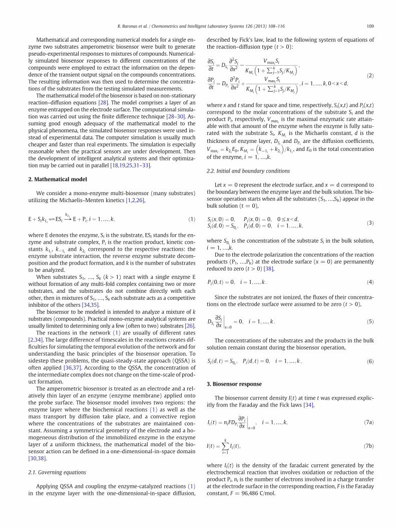
To check the precision of the surrogatemodel of the two-dimensionalbilinear spline type the differences of the values of z(t,c) and ~z t; cð Þ atthe randomly generated points have been computed. The points(shown in Fig. 1) have been generated with uniform distribution over322 = 1024 squares obtained in the discretization of the concentra-tions domain. The maximum of relative error was 3.48 × 10⁻⁵.
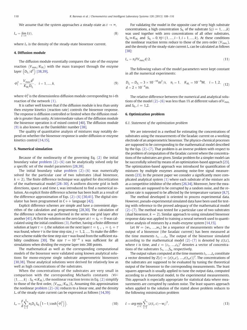
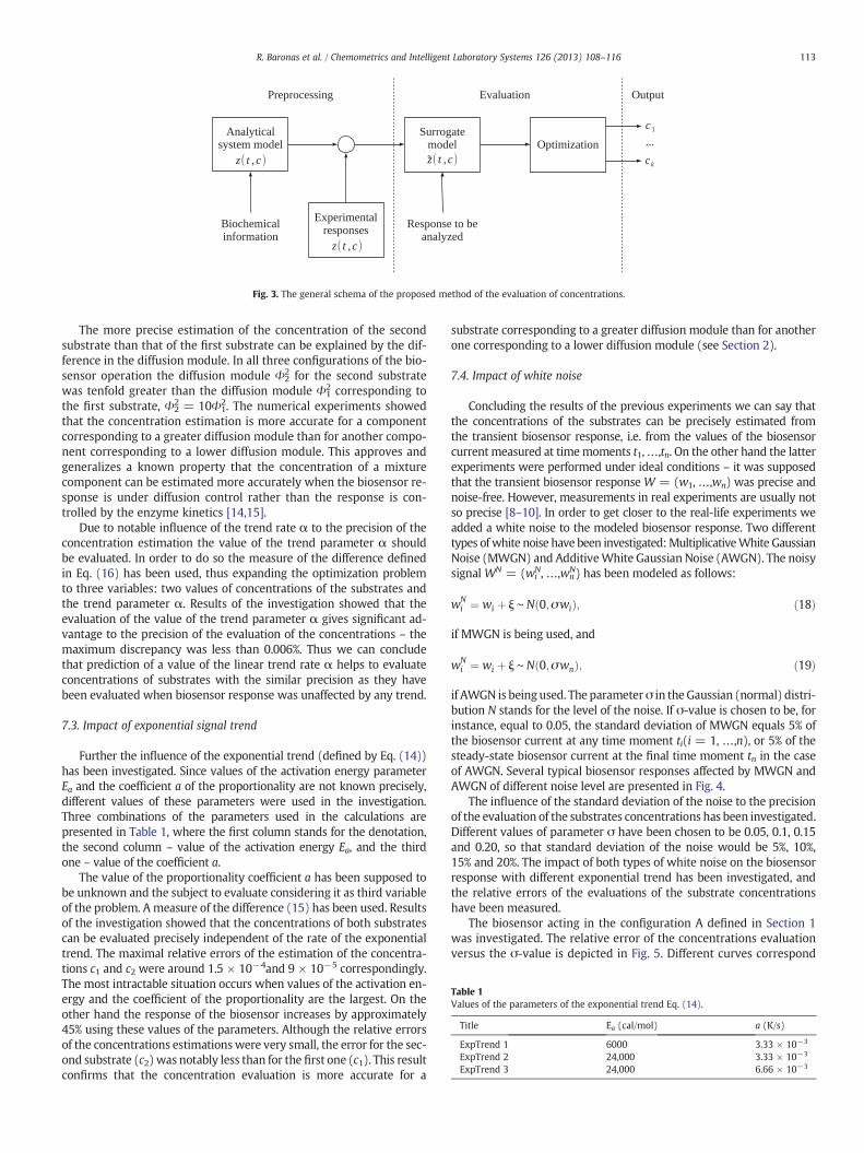
A standard gradient descent method can be applied for the minimi-zation of ~z t; cð Þ, especially because of availability of the analytical for-mula for gradient of ~z t; cð Þ. Moreover the objective functions definedin Section 1 appear unimodal in the region of interest although thatproperty is not provable theoretically; see Fig. 2 for the contour linesof two objective functions corroborating that property. Nevertheless,the computation of minimum point cannot be trivial because of thelarge condition number of Hessian at minimum points of the functionspresented in Fig. 2 which is equal to 0.43 × 10³ and 0.47 × 10⁵
correspondingly.The proposedmethod for the evaluation of the concentrations was
implemented in MATLAB using the local minimization subroutinefmincon. A special MATLAB function has been written to implementformulae defining gradients of the objective functions (14)–(16).
3.2
6.4
9.6
12.8
3.2 6.4 9.6 12.8
c2
c1
Fig. 1. The set of pairs of the dimensionless concentrations of the substrates used inevaluating the precision of the approximation of z(t,c) by ~z t; cð Þ.
112 R. Baronas et al. / Chemometrics and Intelligent Laboratory Systems 126 (2013) 108–116
The stopping condition was defined by the tolerance of functionvalues equal to 10−10, and the tolerance of optimization variableswas equal to 10−5. Taking into account the above-mentioned thelarge condition number of Hessian at minimum points of the objec-tive functions the local descent was repeated three times using ran-domly generated starting points.
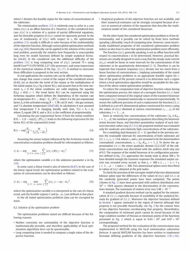
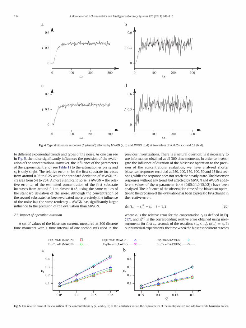
The general schema of the proposed method of the evaluation ofconcentrations is presented in Fig. 3. The biochemical parameters ofthe considered biosensor are used to specify the mathematicalmodel (2)–(7), which in turn is used to compute the values of z(t,c).The preprocessing is a one-time procedure for the considered biosen-sor, and the results of the preprocessing are saved and used by thesubroutine for the computation of values and gradients of ~z t; cð Þ dur-ing the optimization process.
7. Results and discussion
Theworkability of the proposedmethodwas validated by the inves-tigation aimed at the evaluation of concentrations of two substrates in amixture. Then the influence of the linear and exponential trends aswellas of the white noise to the precision of the concentrations estimationwas investigated.
0
5
10
15
20
25a b
0 5 10 15 20 25Low
High
c10 5 10 15 20 25
c1
c2
Fig. 2. Typical contour lines of the objective function when the biosensor response to bothsubstrates (c1 and c2) is controlled by theenzymekinetics (a) andby themass transport (b).
7.1. Method validation
Each component of the mixture was characterized by the individualmaximal enzymatic rate differing in an order of magnitude, while valuesof the Michaelis constant were assumed to be the same (KM1 ¼ KM2 ).Without reducing the generality, it was assumed that themaximal enzy-matic rate for the second substrate is notably greater than for the firstone, Vmax2 ¼ 10Vmax1 . Similar approach was used in a quantitative anal-ysis of mixtures using artificial neural networks [14,15].
Since the analysis quality may depend on whether the biosensorresponse is under the diffusion or the enzyme kinetics control, themaximal enzymatic rates were chosen so that the biosensor wouldoperate under different conditions, i.e. at different values of the diffu-sion modules Φ1
2 and Φ22, keeping Φ2
2 = 10 Φ12.
The following three configurations (A, B and C) of the biosensoroperation were investigated assuming other parameters constant asdefined in Eq. (12):
• The biosensor response to both substrates is controlled by theenzyme kinetics
�Vmax1 ¼ 5� 10−8; Vmax2 ¼ 5� 10−7M=s; Φ2
1≈0:067;Φ2
2≈0:67Þ;• The response is undermixed control (controlled by the enzyme kinet-ics for the first component and bymass transport for the second one),�Vmax1 ¼ 5� 10−7;Vmax2 ¼ 5� 10−6M=s;Φ2
1≈0:67;Φ22≈0:67Þ;
• The mass transport controls the biosensor response to both compo-nents ( Vmax1 ¼ 5� 10−7;Vmax2 ¼ 5� 10−6M=s;Φ2
1≈6:7;Φ22≈6:7
� �.
The first experiment was performed aiming at examination of theinfluence of the implementation precision and the large conditionnumber of the objective functions to the precision of the evaluationof concentrations. The large condition number here means that simi-lar outputs of the biosensor can be obtained for different concentra-tions of the substrates. Therefore a high precision computing of themodel output can be needed for obtaining the sufficient precision ofthe evaluation of the concentrations.
The same set of 1024 pairs of concentrations of the substrates asshown in Fig. 1 has been investigated for each configuration (A, B andC) of the biosensor operation. The feasible region C for the values ofthe normalized concentrations was 0 ≤ c1, c2 ≤ 25.6. In all cases theconcentrations of the mixtures have been evaluated with precisionεi ≤ 4 ⋅ 10−5,
εi ¼ci−~cij jcij j ; i∈ 1;2f g; ð17Þ
where ~c ¼ ~c1; ~c2ð Þ denotes evaluated values, and c = (c1,c2) denotessimulated values of the concentrations. The obtained small relativeerror of the concentrations estimation corroborates the sufficient preci-sion of all numeric algorithms used in implementation of the proposedmethod.
7.2. Impact of linear signal trend
In order to investigate the influence of the signal linear trend to theprecision of the evaluation of the concentrations, a linear trend hasbeen added to the simulated biosensor responses. Three different valuesof the trend parameter α (see (16)) have been chosen so thatthe biosensor current increases by 1%, 3% and 5% in tn seconds of the bio-sensor operation, i.e. at the final moment of the biosensor operation.
Three configurations (A, B and C) of the biosensor operationwere in-vestigated as in the previous experiment. Results of the investigationshowed that the linear trend has significant influence to the error ofthe evaluation of the concentrations – the relative error of the estimatedconcentrations increases up to 33% for the concentration c1 of the firstsubstrate and up to 15% – for the concentration c2 of the second sub-strate, with the largest linear trend rate investigated.
Fig. 3. The general schema of the proposed method of the evaluation of concentrations.
Table 1Values of the parameters of the exponential trend Eq. (14).
Title Ea (cal/mol) a (K/s)
ExpTrend 1 6000 3.33 × 10⁻³
ExpTrend 2 24,000 3.33 × 10⁻³
ExpTrend 3 24,000 6.66 × 10⁻³
113R. Baronas et al. / Chemometrics and Intelligent Laboratory Systems 126 (2013) 108–116
The more precise estimation of the concentration of the secondsubstrate than that of the first substrate can be explained by the dif-ference in the diffusion module. In all three configurations of the bio-sensor operation the diffusion module Φ2
2 for the second substratewas tenfold greater than the diffusion module Φ1
2 corresponding tothe first substrate, Φ2
2 = 10Φ12. The numerical experiments showed
that the concentration estimation is more accurate for a componentcorresponding to a greater diffusion module than for another compo-nent corresponding to a lower diffusion module. This approves andgeneralizes a known property that the concentration of a mixturecomponent can be estimated more accurately when the biosensor re-sponse is under diffusion control rather than the response is con-trolled by the enzyme kinetics [14,15].
Due to notable influence of the trend rate α to the precision of theconcentration estimation the value of the trend parameter α shouldbe evaluated. In order to do so the measure of the difference definedin Eq. (16) has been used, thus expanding the optimization problemto three variables: two values of concentrations of the substrates andthe trend parameter α. Results of the investigation showed that theevaluation of the value of the trend parameter α gives significant ad-vantage to the precision of the evaluation of the concentrations – themaximum discrepancy was less than 0.006%. Thus we can concludethat prediction of a value of the linear trend rate α helps to evaluateconcentrations of substrates with the similar precision as they havebeen evaluated when biosensor response was unaffected by any trend.
7.3. Impact of exponential signal trend
Further the influence of the exponential trend (defined by Eq. (14))has been investigated. Since values of the activation energy parameterEa and the coefficient a of the proportionality are not known precisely,different values of these parameters were used in the investigation.Three combinations of the parameters used in the calculations arepresented in Table 1, where the first column stands for the denotation,the second column – value of the activation energy Ea, and the thirdone – value of the coefficient a.
The value of the proportionality coefficient a has been supposed tobe unknown and the subject to evaluate considering it as third variableof the problem. A measure of the difference (15) has been used. Resultsof the investigation showed that the concentrations of both substratescan be evaluated precisely independent of the rate of the exponentialtrend. The maximal relative errors of the estimation of the concentra-tions c1 and c2 were around 1.5 × 10⁻⁴and 9 × 10⁻⁵ correspondingly.The most intractable situation occurs when values of the activation en-ergy and the coefficient of the proportionality are the largest. On theother hand the response of the biosensor increases by approximately45% using these values of the parameters. Although the relative errorsof the concentrations estimationswere very small, the error for the sec-ond substrate (c2) was notably less than for the first one (c1). This resultconfirms that the concentration evaluation is more accurate for a
substrate corresponding to a greater diffusion module than for anotherone corresponding to a lower diffusion module (see Section 2).
7.4. Impact of white noise
Concluding the results of the previous experiments we can say thatthe concentrations of the substrates can be precisely estimated fromthe transient biosensor response, i.e. from the values of the biosensorcurrentmeasured at timemoments t1,…,tn. On the other hand the latterexperiments were performed under ideal conditions – it was supposedthat the transient biosensor response W = (w1, …,wn) was precise andnoise-free. However, measurements in real experiments are usually notso precise [8–10]. In order to get closer to the real-life experiments weadded a white noise to the modeled biosensor response. Two differenttypes ofwhite noise have been investigated:MultiplicativeWhite GaussianNoise (MWGN) and AdditiveWhite Gaussian Noise (AWGN). The noisysignal WN = (wi
N, …,wnN) has been modeled as follows:
wNi ¼ wi þ ξ∼N 0;σwið Þ; ð18Þ
if MWGN is being used, and
wNi ¼ wi þ ξ∼N 0;σwnð Þ; ð19Þ
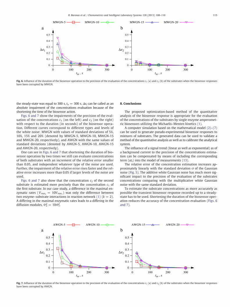
if AWGN is being used. The parameterσ in the Gaussian (normal) distri-bution N stands for the level of the noise. If σ-value is chosen to be, forinstance, equal to 0.05, the standard deviation of MWGN equals 5% ofthe biosensor current at any time moment ti(i = 1, …,n), or 5% of thesteady-state biosensor current at the final time moment tn in the caseof AWGN. Several typical biosensor responses affected by MWGN andAWGN of different noise level are presented in Fig. 4.
The influence of the standard deviation of the noise to the precisionof the evaluation of the substrates concentrations has been investigated.Different values of parameter σ have been chosen to be 0.05, 0.1, 0.15and 0.20, so that standard deviation of the noise would be 5%, 10%,15% and 20%. The impact of both types of white noise on the biosensorresponse with different exponential trend has been investigated, andthe relative errors of the evaluations of the substrate concentrationshave been measured.
The biosensor acting in the configuration A defined in Section 1was investigated. The relative error of the concentrations evaluationversus the σ-value is depicted in Fig. 5. Different curves correspond
0
0.3
0.6
0 100 200 300
I
t,s0 100 200 300
t,s
0 100 200 300t,s
0 100 200 300t,s
0
0.3
0.6
I
0
0.3
0.6
I
0
0.3
0.6
I
a b
c d
Fig. 4. Typical biosensor responses (I, μA/mm2) affected by MWGN (a, b) and AWGN (c, d) at two values of σ: 0.05 (a, c) and 0.2 (b, d).
114 R. Baronas et al. / Chemometrics and Intelligent Laboratory Systems 126 (2013) 108–116
to different exponential trends and types of the noise. As one can seein Fig. 5, the noise significantly influences the precision of the evalu-ation of the concentrations. However, the influence of the parametersof the exponential trend (see Table 1) to the estimation errors ε1 andε2 is only slight. The relative error ε1 for the first substrate increasesfrom around 0.05 to 0.25 while the standard deviation of MWGN in-creases from 5% to 20%. A more significant noise is AWGN – the rela-tive error ε1 of the estimated concentration of the first substrateincreases from around 0.1 to almost 0.45, using the same values ofthe standard deviation of the noise. Although the concentration ofthe second substrate has been evaluated more precisely, the influenceof the noise has the same tendency – AWGN has significantly largerinfluence to the precision of the evaluation than MWGN.
7.5. Impact of operation duration
A set of values of the biosensor current, measured at 300 discretetime moments with a time interval of one second was used in the
0.1
0.2
0.3
0.4
0.05 0.1 0.15 0.2
ε1 ε
σ
a b
ExpTrend1 (MWGN)
ExpTrend2 (MWGN)
ExpTrend3 (MWG
ExpTrend1 (AWG
Fig. 5. The relative error of the evaluation of the concentrations c1 (a) and c2 (b) of the subs
previous investigations. There is a natural question: is it necessary touse information obtained at all 300 time moments. In order to investi-gate the influence of duration of the biosensor operation to the preci-sion of the concentrations evaluation, we have analyzed shorterbiosensor responses recorded at 250, 200, 150, 100, 50 and 25 first sec-onds, while the response does not reach the steady-state. The biosensorresponses without any trend, but affected byMWGN and AWGN at dif-ferent values of the σ-parameter (σ ∈ {0.05,0.1,0.15,0.2}) have beenanalyzed. The influence of the observation time of the biosensor opera-tion to the precision of the evaluation has been expressed by a change inthe relative error,
Δεi tmð Þ ¼ ε mð Þi −εi; i ¼ 1;2; ð20Þ
where εi is the relative error for the concentration ci as defined in Eq.(17), and εi(m) is the corresponding relative error obtained using mea-surements for first tm seconds of the reactions (tm ≤ tn), εi(tn) = εi. Inour numerical experiments, the timewhen the biosensor current reaches
0.1
0.2
0.3
0.4
2
0.05 0.1 0.15 0.2σ
N)
N)
ExpTrend2 (AWGN)
ExpTrend3 (AWGN)
trates versus the σ-parameter of the multiplicative and additive white Gaussian noises.
0
0.1
0.2
0.3
0.4
0.5
0 100 200 300tm , s
0 100 200 300tm , s
MWGN-5 MWGN-10 MWGN-15 MWGN-20
Δ 1ε
0
0.1
0.2
0.3
0.4
0.5
Δ 2ε
a b
Fig. 6. Influence of the duration of the biosensor operation to the precision of the evaluation of the concentrations c1 (a) and c2 (b) of the substrates when the biosensor responseshave been corrupted by MWGN.
115R. Baronas et al. / Chemometrics and Intelligent Laboratory Systems 126 (2013) 108–116
the steady-state was equal to 300 s, tn = 300 s. Δεi can be called as anabsolute impairment of the concentrations evaluation because of theshortening the time of the biosensor action.
Figs. 6 and 7 show the impairments of the precision of the eval-uation of the concentrations c1 (on the left) and c2 (on the right)with respect to the duration (in seconds) of the biosensor opera-tion. Different curves correspond to different types and levels ofthe white noise: MWGN with values of standard deviations of 5%,10%, 15% and 20% (denoted by MWGN-5, MWGN-10, MWGN-15and MWGN-20, respectively), and AWGN with the same values ofstandard deviations (denoted by AWGN-5, AWGN-10, AWGN-15and AWGN-20, respectively).
One can see in Figs. 6 and 7 that shortening the duration of bio-sensor operation by two times we still can evaluate concentrationsof both substrates with an increment of the relative error smallerthan 0.05, and independent whatever type of the noise are used.Further, the impairment of the relative error rises faster and the rel-ative error increases more than 0.05 if larger levels of the noise areused.
Figs. 6 and 7 also show that the concentration c2 of the secondsubstrate is estimated more precisely than the concentration c1 ofthe first substrate. In our case study, a difference in the maximal en-zymatic rates (Vmax2 = 10Vmax1 ) was only the difference betweentwo enzyme–substrate interactions in reaction network (1) (k = 2).A differing in the maximal enzymatic rates leads to a differing in thediffusion modules, Φ2
2 = 10Φ12.
0
0.1
0.2
0.3
0.4
0.5
0 100 200 300tm , s
AWGN-5 AWGN-10
Δ 1ε Δ
a
Fig. 7. Influence of the duration of the biosensor operation to the precision of the evaluationhave been corrupted by AWGN.
8. Conclusions
The proposed optimization-based method of the quantitativeanalysis of the biosensor response is appropriate for the evaluationof the concentrations of the substrates by single enzyme amperomet-ric biosensors utilizing the Michaelis–Menten kinetics (1).
A computer simulation based on the mathematical model (2)–(7)can be used to generate pseudo-experimental biosensor responses tomixtures of substrates. The generated data can be used to validate amethod of the quantitative analysis as well as to calibrate the analyticalsystem.
The influence of a signal trend (linear as well as exponential) as ofa background current to the precision of the concentrations estima-tion can be compensated by means of including the correspondingterm (ati) into the model of measurements (13).
The relative error of the concentration estimation increases ap-proximately linearly with the standard deviation σ of the Gaussiannoise (Fig. 5). The additive white Gaussian noise has much more sig-nificant impact to the precision of the evaluation of the substratesconcentrations comparing with the multiplicative white Gaussiannoise with the same standard deviation.
To estimate the substrate concentrations as more accurately aspossible the transient biosensor response recorded up to a steady-state has to be used. Shortening the duration of the biosensor oper-ation reduces the accuracy of the concentration evaluation (Figs. 6and 7).
AWGN-15 AWGN-20
0
0.1
0.2
0.3
0.4
0.5
0 100 200 300tm , s
2ε
b
of the concentrations c1 (a) and c2 (b) of the substrates when the biosensor responses
116 R. Baronas et al. / Chemometrics and Intelligent Laboratory Systems 126 (2013) 108–116
The concentration estimation ismore accurate for a substrate (c2) cor-responding to a greater diffusion module than for another substrate (c1)corresponding to a lower diffusion module (Figs. 5–7). Particularly, theconcentration of amixture component can be estimatedmore accuratelywhen the biosensor response is under diffusion control for this compo-nent rather than the response is controlled by the enzyme kinetics.
Acknowledgments
This research is funded by the European Social Fund under the GlobalGrant measure, Project No. VP1-3.1-ŠMM-07-K-01-073/MTDS-110000-583.
References
[1] In: A.P.F. Turner, I. Karube, G.S. Wilson (Eds.), Biosensors: Fundamentals and Ap-plications, Oxford University Press, Oxford, 1990.
[2] F.W. Scheller, F. Schubert, Biosensors, Elsevier Science, Amsterdam, 1992.[3] F.-G. Banica, Chemical Sensors and Biosensors: Fundamentals and Applications,
John Wiley & Sons, Chichester, 2012.[4] D. Grieshaber, R. MacKenzie, J. Vörös, E. Reimhult, Electrochemical biosensors —
sensor principles and architectures, Sensors 8 (2008) 1400–1458.[5] A. de Juan, R. Tauler, Chemometrics applied to unravel multicomponent processes
and mixtures. Revisiting latest trends in multivariate resolution, Analytica ChimicaActa 500 (2003) 195–210.
[6] A. de Juan, R. Tauler,Multivariate curve resolution (mcr) from2000: progress in con-cepts and applications, Critical Reviews in Analytical Chemistry 36 (2006) 163–176.
[7] P.K. Hopke, The evolution of chemometrics, Analytica Chimica Acta 500 (2003)365–377.
[8] Z. Wu, N.E. Huang, S.R. Long, C.-K. Peng, On the trend, detrending, and variabilityof nonlinear and nonstationary time series, Proceedings of the National Academyof Sciences of the United States of America 104 (2007) 14889–14894.
[9] A. Hassibi, H. Vikalo, A. Hajimiri, On noise processes and limits of performance inbiosensors, Journal of Applied Physics 102 (2007) 014909.
[10] R. Merletti, A. Botter, A. Troiano, E. Merlo, M.A. Minetto, Technology and instru-mentation for detection and conditioning of the surface electromyographic sig-nal: state of the art, Clinical biomechanics 24 (2009) 122–134.
[11] R.S. Freire, M.M. Ferreira, N. Durán, L.T. Kubota, Dual amperometric biosensor de-vice for analysis of binary mixtures of phenols by multivariate calibration usingpartial least squares, Analytica Chimica Acta 485 (2003) 263–269.
[12] E. Tønning, S. Sapelnikova, J. Christensen, C. Carlsson, M. Winther-Nielsen, E.Dock, R. Solna, P. Skladal, L. Nørgaard, T. Ruzgas, J. Emnéus, Chemometric explo-ration of an amperometric biosensor array for fast determination of wastewaterquality, Biosensors and Bioelectronics 21 (2005) 608–615.
[13] A.V. Lobanov, I.A. Borisov, S.H. Gordon, R.V. Greene, T.D. Leathers, A.N. Reshetilov,Analysis of ethanol–glucose mixtures by two microbial sensors: application ofchemometrics and artificial neural networks for data processing, Biosensors andBioelectronics 16 (2001) 1001–1007.
[14] R. Baronas, F. Ivanauskas, R. Maslovskis, P. Vaitkus, An analysis of mixtures usingamperometric biosensors and artificial neural networks, Journal of MathematicalChemistry 36 (2004) 281–297.
[15] R. Baronas, F. Ivanauskas, R. Maslovskis, M. Radavičius, P. Vaitkus, Locally weightedneural networks for an analysis of the biosensor response, Kybernetika 43 (2007)21–30.
[16] G.A. Alonso, G. Istamboulie, T. Noguer, J.-L. Marty, R. Muñoz, Rapid determinationof pesticide mixtures using disposable biosensors based on genetically modifiedenzymes and artificial neural networks, Sensors and Actuators B: Chemical 164(2012) 22–28.
[17] T. Danzer, G. Schwedt, Chemometric methods for the development of a biosensorsystem and the evaluation of inhibition studies with solutions and mixtures ofpesticides and heavy metals part 1: development of an enzyme electrodes systemfor pesticide and heavy metal screening using selected chemometric methods,Analytica Chimica Acta 318 (1996) 275–286.
[18] V. Flexer, K. Pratt, F. Garay, P. Bartlett, E. Calvo, Relaxation and simplex mathe-matical algorithms applied to the study of steady-state electrochemical responsesof immobilized enzyme biosensors: comparison with experiments, Journal ofElectroanalytical Chemistry 616 (2008) 87–98.
[19] F.R.P. Oliveira, K. Goldberg, A. Liese, B. Hitzmann, Chemometric modelling for pro-cess analyzers using just a single calibration sample, Chemometrics and Intelli-gent Laboratory Systems 94 (2008) 118–122.
[20] K. Shoorideh, C.O. Chui, Optimization of the sensitivity of fet-based biosensors via bi-asing and surface charge engineering, IEEE Transactions Electron Devices 59 (2012)3104–3110.
[21] M.R. Sohrabi, S. Jamshidi, A. Esmaeilifar, Cloud point extraction for determinationof diazinon: optimization of the effective parameters using taguchi method,Chemometrics and Intelligent Laboratory Systems 110 (2012) 49–54.
[22] V. Privman, G. Strack, D. Solenov, M. Pita, E. Katz, Optimization of enzymatic bio-chemical logic for noise reduction and scalability: how many biocomputinggates can be interconnected in a circuit? The Journal of Physical Chemistry. B112 (2008) 11777–11784.
[23] A. Žilinskas, D. Baronas, Optimization-based evaluation of concentrations inmodeling the biosensor-aided measurement, Informatica 22 (2011) 589–600.
[24] L. Pasti, B. Walczak, D.L. Massart, P. Reschiglian, Optimization of signal denoisingin discrete wavelet transform, Chemometrics and Intelligent Laboratory Systems48 (1999) 21–34.
[25] E. Katz, V. Bocharova, M. Privman, Electronic interfaces switchable by logicallyprocessed multiple biochemical and physiological signals, Journal of MaterialsChemistry 22 (2012) 8171–8178.
[26] T. Pocklington, J. Jeffery, Competition of two substrates for a single enzyme. Asimple kinetic theorem exemplified by a hydroxy steroid dehydrogenase reac-tion, Biochemical Journal 112 (1969) 331–334.
[27] R.Wilson, A. Turner, Glucose oxidase: an ideal enzyme, Biosensors and Bioelectronics 7(1992) 165–185.
[28] D. Britz, Digital Simulation in Electrochemistry, 3rd edition Springer, Berlin, 2005.[29] D. Britz, R. Baronas, E. Gaidamauskaitė, F. Ivanauskas, Further comparisons of fi-
nite difference schemes for computational modelling of biosensors, NonlinearAnalysis Modelling and Control 14 (2009) 419–433.
[30] R. Baronas, F. Ivanauskas, J. Kulys, Mathematical Modeling of Biosensors, Springer,Dordrecht, 2010.
[32] F. Ataíde, B. Hitzmann, When is optimal experimental design advantageous forthe analysis of Michaelis–Menten kinetics? Chemometrics and Intelligent Labora-tory Systems 99 (2009) 9–18.
[33] O.V. Klymenko, C. Amatore,W. Sun, Y.-L. Zhou, Z.-W. Tian, I. Svir, Theory and compu-tational study of electrophoretic ion separation and focusing in microfluidic chan-nels, Nonlinear Analysis Modelling and Control 17 (2012) 431–447.
[34] H. Gutfreund, Kinetics for the Life Sciences, Cambridge University Press, Cam-bridge, 1995.
[35] J. Kulys, R. Baronas, Modelling of amperometric biosensors in the case of substrateinhibition, Sensors 6 (2006) 1513–1522.
[36] L.A. Segel, M. Slemrod, The quasi-steady-state assumption: a case study in pertur-bation, SIAM Review 31 (1989) 446–477.
[37] B. Li, Y. Shen, B. Li, Quasi-steady-state laws in enzyme kinetics, Journal of PhysicalChemistry A 112 (2008) 2311–2321.
[38] T. Schulmeister, Mathematical modelling of the dynamic behaviour of ampero-metric enzyme electrodes, Selective Electrode Reviews 12 (1990) 203–260.
[39] J. Kulys, The development of new analytical systems based on biocatalysts, Ana-lytical Letters 14 (1981) 377–397.
[40] R. Baronas, J. Kulys, F. Ivanauskas, Modelling amperometric enzyme electrode withsubstrate cyclic conversion, Biosensors and Bioelectronics 19 (2004) 915–922.
[41] E. Gaidamauskaitė, R. Baronas, A comparison of finite difference schemes for com-putational modelling of biosensors, Nonlinear Analysis Modelling and Control 12(2007) 359–369.
[43] A. Törn, A. Žilinskas, Global optimization, Lecture Notes in Computer Science 350(1989) 1–255.
[44] A. Žilinskas, J. Žilinskas, Interval arithmetic based optimization in nonlinear re-gression, Informatica 21 (2010) 149–158.
[45] A. Žilinskas, J. Žilinskas, A hybrid global optimization algorithm for non-linearleast squares regression, Journal of Global Optimization (2012), http://dx.doi.org/10.1007/s10898-011-9840-9.
[46] Y. Bao, W. Kong, Y. He, F. Liu, T. Tian, W. Zhou, Quantitative analysis of total aminoacid in barley leaves under herbicide stress using spectroscopic technology andchemometrics, Sensors 12 (2012) 13393–13401.
[47] M. Wickramasinghe, I.Z. Kiss, Effect of temperature on precision of chaotic oscil-lations in nickel electrodissolution, Chaos 20 (2010) 023125.
[48] I. Fabrikant, H. Hotop, On the validity of the Arrhenius equation for electron at-tachment rate coefficients, Journal of Chemical Physics 128 (2008) 124308.