Optimization using optim() in R - Erik Erhardt · Chapter 1 Optimization using optim() in R An...

Chapter 1

Optimization usingoptim() in R

An in-class activity to apply Nelder-Mead and Simulated Annealing in

optim() for a variety of bivariate functions.# SC1 4/18/2013

# Everyone optim()!

# The goal of this exercise is to minimize a function using R's optim().

# Steps:

# 0. Break into teams of size 1 or 2 students.

# 1. Each team will choose a unique function from this list:

# Test functions for optimization

# http://en.wikipedia.org/wiki/Test_functions_for_optimization

# 1a. Claim the function by typing your names into the function section below.

# 1b. Click on "edit" on Wikipedia page to copy latex math for function

# and paste between dollar signs £f(x)£

# 2. Following my "Sphere function" example:

# 2a. Define function()

# 2b. Plot the function

# 2c. Optimize (minimize) the function

# 2d. Comment on convergence

# 3. Paste your work into your function section.

# 4. I'll post this file on the website for us all to enjoy, as well as create

# a lovely pdf with images of the functions.

2 Optimization using optim() in R

1.1 Sphere function

f (x) =∑n

i=1 x2i

########################################

# Sphere function

# Erik Erhardt

# £f(\boldsymbol{x}) = \sum_{i=1}^{n} x_{i}^{2}£

# name used in plot below

f.name <- "Sphere function"

# define the function

f.sphere <- function(x) {# make x a matrix so this function works for plotting and for optimizing

x <- matrix(x, ncol=2)

# calculate the function value for each row of x

f.x <- apply(x^2, 1, sum)

# return function value

return(f.x)

}

# plot the function

# define ranges of x to plot over and put into matrix

x1 <- seq(-10, 10, length = 101)

x2 <- seq(-10, 10, length = 101)

X <- as.matrix(expand.grid(x1, x2))

colnames(X) <- c("x1", "x2")

# evaluate function

y <- f.sphere(X)

# put X and y values in a data.frame for plotting

df <- data.frame(X, y)

# plot the function

library(lattice) # use the lattice package

wireframe(y ~ x1 * x2 # y, x1, and x2 axes to plot

, data = df # data.frame with values to plot

, main = f.name # name the plot

, shade = TRUE # make it pretty

, scales = list(arrows = FALSE) # include axis ticks

, screen = list(z = -50, x = -70) # view position

)

# optimize (minimize) the function using Nelder-Mead

out.sphere <- optim(c(1,1), f.sphere, method = "Nelder-Mead")

1.1 Sphere function 3

out.sphere

## $par

## [1] 3.754010e-05 5.179101e-05

##

## $value

## [1] 4.091568e-09

##

## $counts

## function gradient

## 63 NA

##

## $convergence

## [1] 0

##

## $message

## NULL

# optimize (minimize) the function using Simulated Annealing

out.sphere <- optim(c(1,1), f.sphere, method = "SANN")

out.sphere

## $par

## [1] 0.0001933246 -0.0046279762

##

## $value

## [1] 2.145554e-05

##

## $counts


## 10000 NA

##

## $convergence

## [1] 0

##

## $message

## NULL

###

# comments based on plot and out.*

# The unique minimum was found within tolerance.

## values of x1 and x2 at the minimum

# £par

# [1] 3.754010e-05 5.179101e-05

#


## value of the function at the minimum

# £value

# [1] 4.091568e-09

#

## convergence in 63 iterations

# £counts

# function gradient

# 63 NA

#

## 0 = convergence successful

# £convergence

# [1] 0

#

## no news is good news

# £message

# NULL

Sphere function

−10

−5

0

5

10 −10

−5

05

10

0

50

100

150

200

x1x2

y

1.2 Sphere function with stochastic noise 5

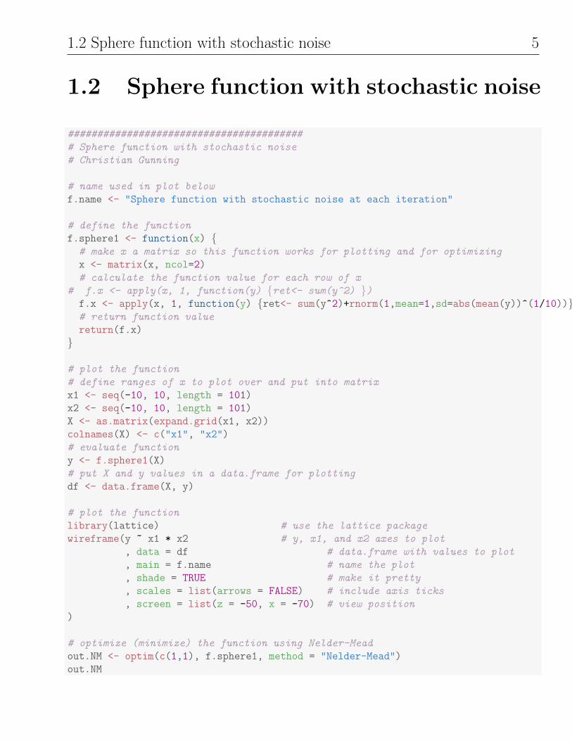
1.2 Sphere function with stochastic noise

########################################

# Sphere function with stochastic noise

# Christian Gunning


f.name <- "Sphere function with stochastic noise at each iteration"


f.sphere1 <- function(x) {# make x a matrix so this function works for plotting and for optimizing



# f.x <- apply(x, 1, function(y) {ret<- sum(y^2) })f.x <- apply(x, 1, function(y) {ret<- sum(y^2)+rnorm(1,mean=1,sd=abs(mean(y))^(1/10))})# return function value

return(f.x)

}

# plot the function


x1 <- seq(-10, 10, length = 101)

x2 <- seq(-10, 10, length = 101)



# evaluate function

y <- f.sphere1(X)



# plot the function








)


out.NM <- optim(c(1,1), f.sphere1, method = "Nelder-Mead")

out.NM


## $par

## [1] 0.875 1.150

##

## $value

## [1] 0.2254641

##

## $counts


## 321 NA

##

## $convergence

## [1] 10

##

## $message

## NULL


out.sann <- optim(c(1,1), f.sphere1, method = "SANN")

out.sann

## $par

## [1] -0.7529075 -0.3134403

##

## $value

## [1] -1.036117

##

## $counts


## 10000 NA

##

## $convergence

## [1] 0

##

## $message

## NULL

1.2 Sphere function with stochastic noise 7

Sphere function with stochastic noise at each iteration

−10

−5

0

5

10 −10

−5

05

10

0

50

100

150

200

x1x2

y


1.3 Goldstein-Price function

f (x, y) =(

1 + (x + y + 1)2(19− 14x + 3x2 − 14y + 6xy + 3y2

))×(

30 + (2x− 3y)2(18− 32x + 12x2 + 48y − 36xy + 27y2

))########################################

# Goldstein-Price function

# Andisheh/Jerry


f.name <- "Goldstein Price function"


f.GP <- function(x) {# make x a matrix so this function works for plotting and for optimizing


x1<-x[,1]

x2<-x[,2]


f.xy <- ((1+((x1+x2+1))^(2)*((19-14*x1+3*x1^(2)-14*x2+6*x1*x2+3*x2^(2)))))*((30+((2*x1-3*x2))^(2)*((18-32*x1+12*x1^(2)+48*x2-36*x1*x2+27*x2^(2)))))


return(f.xy)

}x1 <- seq(-3, 3, length = 101)

x2 <- seq(-3, 3, length = 101)

# plot the function




# evaluate function

y <- f.GP(X)


df <- data.frame(X,y)

# plot the function








1.3 Goldstein-Price function 9

)


out.sphere <- optim(c(1,1), f.GP, method = "Nelder-Mead")

out.sphere

## $par

## [1] 1.2000535 0.8000135

##

## $value

## [1] 840

##

## $counts


## 55 NA

##

## $convergence

## [1] 0

##

## $message

## NULL


out.sphere <- optim(c(1,1), f.GP, method = "SANN")

out.sphere

## $par

## [1] 1.8017918 0.2004454

##

## $value

## [1] 84.00537

##

## $counts


## 10000 NA

##

## $convergence

## [1] 0

##

## $message

## NULL


Goldstein Price function

−3−2

−10

12

3 −3−2

−10

12

3

1e+06

2e+06

3e+06

4e+06

x1x2

y

1.4 Booth’s function 11

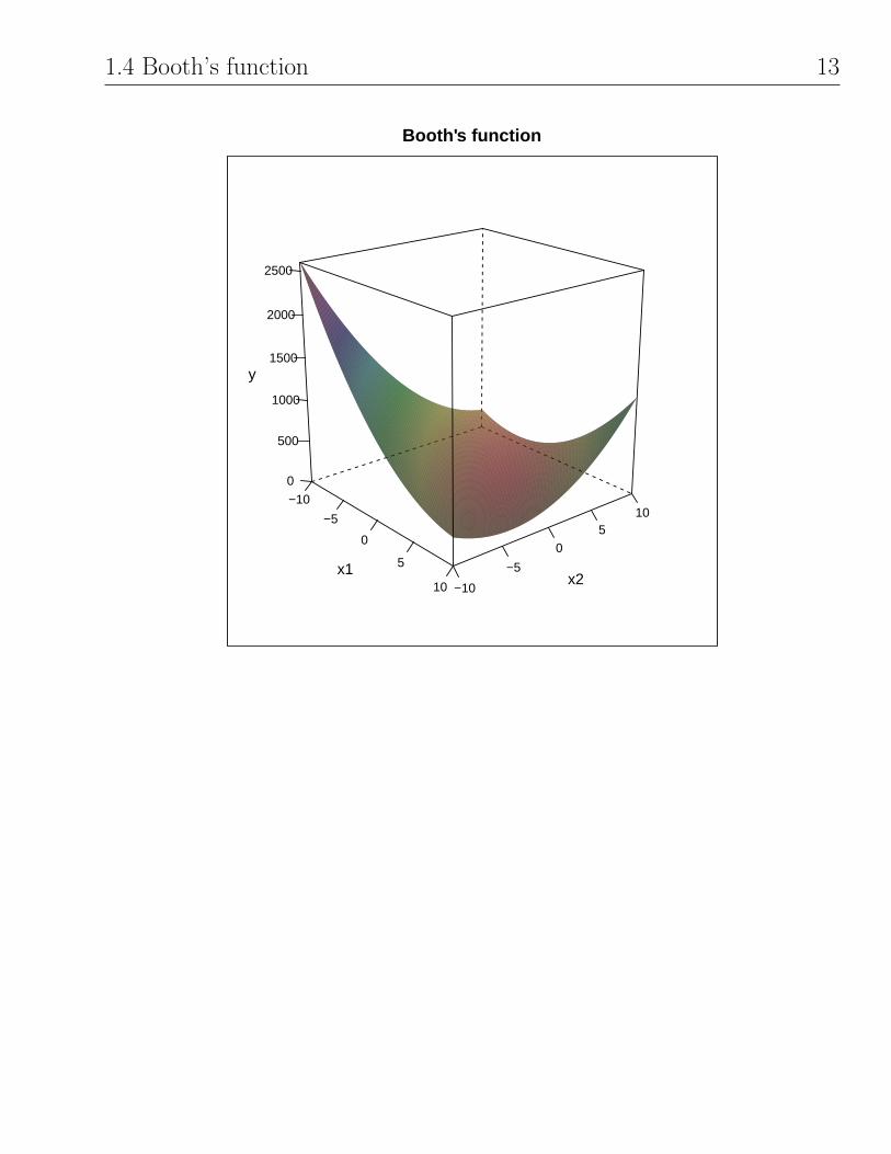
1.4 Booth’s function

f (x) = (x + 2y − 7)2 + (2x + y − 5)2

########################################

# Booth's function

#

# Mina Lee, Flor like a flower

f.name <- "Booth's function"


f.booth <- function(x) {# make x a matrix so this function works for plotting and for optimizing



f.x <- (( x[,1] + 2*x[,2] -7)^{2} + (2*x[,1] +x[,2] - 5)^{2} )


return(f.x)

}

# plot the function


x1 <- seq(-10, 10, length = 101)

x2 <- seq(-10, 10, length = 101)



# evaluate function

y <- f.booth(X)



# plot the function








)


out.booth <- optim(c(1,1), f.booth, method = "Nelder-Mead")

out.booth


## $par

## [1] 0.9998584 3.0001488

##

## $value

## [1] 4.239191e-08

##

## $counts


## 69 NA

##

## $convergence

## [1] 0

##

## $message

## NULL


out.booth <- optim(c(1,1), f.booth, method = "SANN")

out.booth

## $par

## [1] 0.996048 3.003057

##

## $value

## [1] 2.816719e-05

##

## $counts


## 10000 NA

##

## $convergence

## [1] 0

##

## $message

## NULL

1.4 Booth’s function 13

Booth's function

−10

−5

0

5

10 −10

−5

05

10

0

500

1000

1500

2000

2500

x1x2

y


1.5 Eggholder function

f (x, y) = − (y + 47) sin(√∣∣y + x

2 + 47∣∣)− x sin

(√|x− (y + 47)|

)########################################

# Eggholder function

# Stefan and John


f.name <- "Eggholder function"

# make the function

f.egg<- function(x){-(x[,2]+47)*sin(sqrt(abs(x[,2]+(x[,1]/2)+47)))-x[,1]*sin(sqrt(abs(x[,1]-(x[,2]+47))))

}


f.egghold <- function(x) {# make x a matrix so this function works for plotting and for optimizing



f.x <- f.egg(x)


return(f.x)

}

# plot the function


x1 <- seq(-512, 512, length = 101)

x2 <- seq(-512, 512, length = 101)



# evaluate function

y <- f.egghold(X)



# plot the function






1.5 Eggholder function 15



)


out.egghold <- optim(c(500,400), f.egghold, method = "Nelder-Mead")

out.egghold

## $par

## [1] 482.3553 432.8814

##

## $value

## [1] -956.9182

##

## $counts


## 93 NA

##

## $convergence

## [1] 0

##

## $message

## NULL


out.egghold <- optim(c(500,400), f.egghold, method = "SANN")

out.egghold

## $par

## [1] 522.1702 413.3341

##

## $value

## [1] -976.9109

##

## $counts


## 10000 NA

##

## $convergence

## [1] 0

##

## $message

## NULL

###

# comments based on plot and out.*




# £par

# [1] 522.1324 413.3086

#


# £value

# [1] -976.9105

#


# £counts

# function gradient

# 63 NA

#


# £convergence

# [1] 10000

#


# £message

# NULL

1.5 Eggholder function 17

Eggholder function

−400

−200

0

200

400

−400 −200 0 200 400

−500

0

500

1000

x1

x2

y


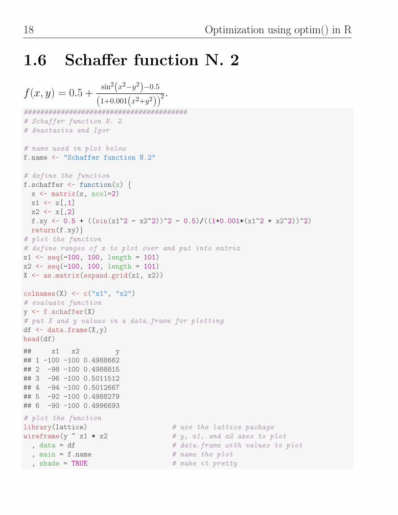
1.6 Schaffer function N. 2

f (x, y) = 0.5 +sin2(x2−y2)−0.5

(1+0.001(x2+y2))2 .

########################################

# Schaffer function N. 2

# Anastasiia and Igor


f.name <- "Schaffer function N.2"


f.schaffer <- function(x) {x <- matrix(x, ncol=2)

x1 <- x[,1]

x2 <- x[,2]

f.xy <- 0.5 + ((sin(x1^2 - x2^2))^2 - 0.5)/((1+0.001*(x1^2 + x2^2))^2)

return(f.xy)}# plot the function


x1 <- seq(-100, 100, length = 101)

x2 <- seq(-100, 100, length = 101)



# evaluate function

y <- f.schaffer(X)


df <- data.frame(X,y)

head(df)

## x1 x2 y

## 1 -100 -100 0.4988662

## 2 -98 -100 0.4988815

## 3 -96 -100 0.5011512

## 4 -94 -100 0.5012667

## 5 -92 -100 0.4988279

## 6 -90 -100 0.4996693

# plot the function






1.6 Schaffer function N. 2 19



)


out.schaffer <- optim(c(1,1), f.schaffer, method = "Nelder-Mead")

out.schaffer

## $par

## [1] 9.811556e-05 1.267615e-05

##

## $value

## [1] 9.787393e-12

##

## $counts


## 99 NA

##

## $convergence

## [1] 0

##

## $message

## NULL



## £par

## [1] 9.811556e-05 1.267615e-05

##


## £value

## [1] 9.787393e-12

##


## £counts


## 99 NA

##


## £convergence

## [1] 0

##


## £message

## NULL


Schaffer function N.2

−100

−50

0

50

100−100

−50

050

100

0.0

0.2

0.4

0.6

0.8

x1x2

y

1.7 Styblinski-Tang function 21

1.7 Styblinski-Tang function

f (x) =∑n

i=1 x4i−16x

2i+5xi

2 .########################################

# Styblinski-Tang function

# Miao Yu and Xin Wang

########################################


f.name <-"Tang function"


f.tang <- function(x) {# make x a matrix so this function works for plotting and for optimizing



f.x <- apply(x^4-16*x^2+5*x, 1, sum)/2


return(f.x)

}

# plot the function


x1 <- seq(-5, 5, length = 101)

x2 <- seq(-5, 5, length = 101)



# evaluate function

y <- f.tang(X)



# plot the function








)



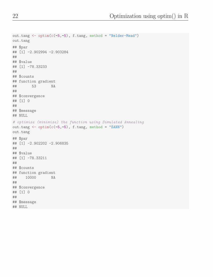
out.tang <- optim(c(-5,-5), f.tang, method = "Nelder-Mead")

out.tang

## $par

## [1] -2.902994 -2.903284

##

## $value

## [1] -78.33233

##

## $counts


## 53 NA

##

## $convergence

## [1] 0

##

## $message

## NULL


out.tang <- optim(c(-5,-5), f.tang, method = "SANN")

out.tang

## $par

## [1] -2.902202 -2.906835

##

## $value

## [1] -78.33211

##

## $counts


## 10000 NA

##

## $convergence

## [1] 0

##

## $message

## NULL

1.7 Styblinski-Tang function 23

Tang function

−4

−2

0

2

4 −4

−2

0

2

4

−50

0

50

100

150

200

250

x1x2

y

Date post:	29-Apr-2018
Category:	Documents
Upload:	lamque
View:	234 times
Download:	0 times

Optimization using optim() in R - Erik Erhardt · Chapter 1 Optimization using optim() in R An...

Documents