i

Optimized Design of Axially Symmetric Cassegrain Reflector antenna using Iterative

Local Search Algorithm

A THESIS SUBMITTED IN PARTIAL FULFILLMENT

OF THE REQUIREMENTS FOR THE DEGREE OF

Master of Technology

In

Electronics Systems and Communication

By

OBULESU DANDU

211EE1116

Department of Electrical Engineering

National Institute of Technology, Rourkela

Rourkela-769008

ii

Optimized Design of Axially Symmetric Cassegrain Reflector antenna using Iterative

Local Search Algorithm

A THESIS SUBMITTED IN PARTIAL FULFILLMENT

OF THE REQUIREMENTS FOR THE DEGREE OF

Master of Technology

In

Electronics Systems and Communication

By

OBULESU DANDU

211EE1116

Under the Guidance of

Prof. K.R.SUBHASHINI

Department of Electrical Engineering

National Institute of Technology, Rourkela

Rourkela-769008

iii

Department of Electrical Engineering

National Institute of Technology Rourkela

CERTIFICATE

This is to certify that the thesis entitled, “Optimized Design of Axially Symmetric

Cassegrain Reflector Antenna using Iterative Local Search Algorithm” submitted by Mr.

Obulesu Dandu in partial fulfillment of the requirements for the award of Master of

Technology Degree in electrical Engineering with specialization in “Electronics Systems and

Communication” during session 2011-13 at the National Institute of Technology, Rourkela

(Deemed University) is an authentic work carried out by him under my supervision and

guidance.

To the best of my knowledge, the matter embodied in the thesis has not been submitted to any

other University/ Institute for the award of any degree or diploma.

Date: Prof. K.R.Subhashini

Department of Electrical Engineering

National Institute of Technology

Rourkela-769008

iv

ACKNOWLEDGEMENTS

This project is by far the most significant accomplishment in my life and it would be

impossible without people who supported me and believed in me.

I would like to extend my gratitude and my sincere thanks to my supervisor Prof.

K.R.Subhashini, Department of Electrical Engineering. I express my gratitude to faculties

Professors P.K.SAHOO, D. PATRA , S.DAS for their advices during inter evaluation.

I am very much thankful to our Head of the Department, Prof. A.K.Panda, for

providing us with best facilities in the department and his timely suggestions. I am very much

thankful for providing valuable suggestions during my thesis work to all my teachers in the

Department. They have been great sources of inspiration to me and I thank them from the

bottom of my heart.

I would like to thank DONDAPATI.SUNEEL VARMA, BANDARU SRINIVASA

RAO and K.VENKATESWARA RAO for their support and suggestions during problem

solving.

I would like to thank all my friends and especially my classmates for all the thoughtful

and mind stimulating discussions we had, which prompted us to think beyond the obvious. I’ve

enjoyed their companionship so much during my stay at NIT, Rourkela.

I would like to thank all those who made my stay in Rourkela an unforgettable and

rewarding experience.

Last but not least I would like to thank my parents, who taught me the value of hard

work by their own example. They rendered me enormous support being apart during the whole

tenure of my stay in NIT Rourkela.

Obulesu Dandu

v

TABLE OF CONTENT

1 INTRODUCTION AND SCOPE OF THE PROJECT

1

1.1 Objective 2

1.2 Motivation 2

1.3 Introduction 3

1.4 Specifications of 18.5 GHz Reflector Antenna 4

1.5 Aim of the project 4

1.6 Organization of Thesis 5

2 CASSEGRAIN ANTENNA CONFIGURATION

6

2.1 Introduction

7

2.1.1 Advantages 7

2.2 Cassegrain Antenna Design 8

2.2.1 Cassegrain Antenna Design Parameters 8

2.3 Parabolic Reflector 9

2.4 Parabolic Reflector Design 10

2.4.1 Geometry 10

2.4.2 f/D Ratio 11

2.4.3 Electrical and Mechanical considerations for f/D Ratio 12

2.5 Dish Illumination 13

2.6 Advantages of Parabolic Reflectors 13

2.7 Shroud 13

2.8 Cassegrain Sub Reflector 14

2.9 Feed Horn Design

2.9.1 Waveguide Horn

16

16

2.10 Radome 19

2.11 18.5 GHz Main Reflector Design Values 20

2.12 Main Reflector Contour Co-ordinates 21

2.13 18 GHz Cassegrain Sub Reflector Design 21

2.14 Sub Reflector Contour Co-ordinates 23

2.15 Summary 23

vi

3 ITERATIVE LOCAL SEARCH ALGORITHM 24

3.1 Iterated Local Search algorithm

3.1.1 Strategy

25

25

3.1.2 Pseudo code for Iterated Local Search. 25

3.1.3 Heuristics 26

4. ANALYSIS OF CASSEGRAIN ANTENNA USING GRASP SOFTWARE 27

4.1 Introduction 28

4.2 Dual Reflector Blockage 29

4.3 Subreflector Blockage 30

4.4 Visualizing the Geometry 30

4.4.1 Visualizing the geometry as an open loop GL plot 31

4.4.2 Visualizing the geometry as an open loop Object plot 31

4.4.3 Radiation Pattern 32

4.5 Summary

36

4.6 Aluminum alloys-Advantages 36

4.7 RF Absorber -Advantages 37

5 RESULTS

38-43

6 CONCLUSION AND FUTURE WORK 44

6.1 Conclusions 45

6.2 Future Scope of the Project 45

REFERENCES 46-47

vii

LIST OF FIGURES

2.1 2-D CAD view of Cassegrain Antenna

8

2.2 Cassegrain Antenna Edge Taper

12

2.3 CAD Parabolic Reflector Contour 13

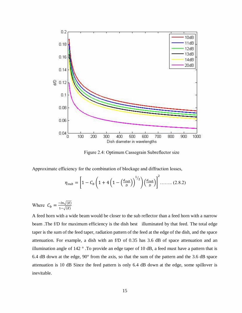
2.4 Optimum Cassegrain subreflector size 15

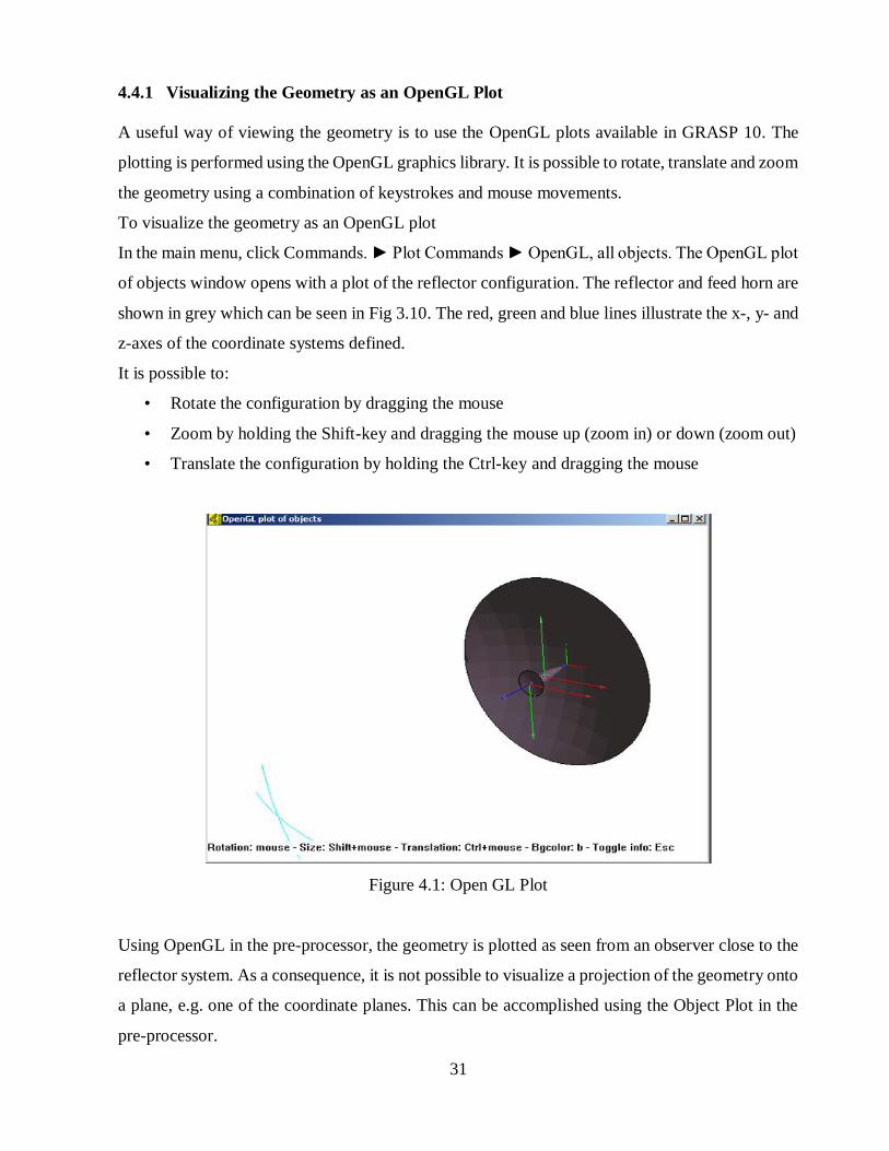
4.1 Open GL plot

31

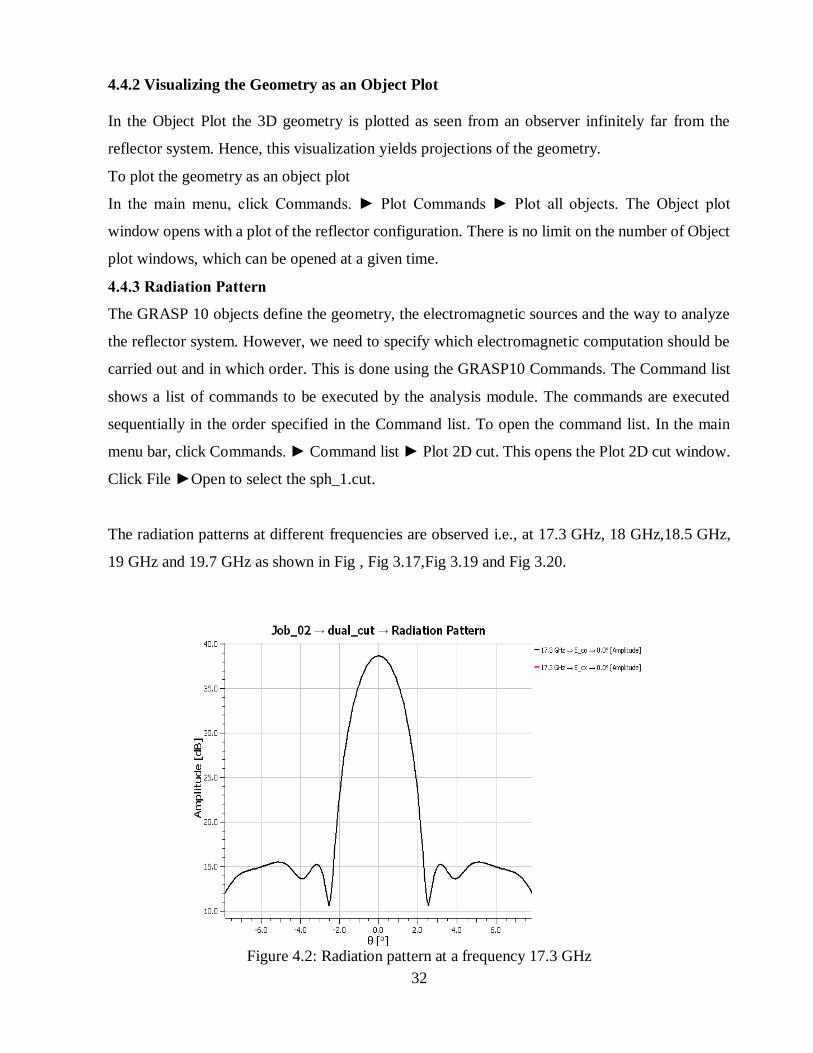
4.2 Radiation pattern at a frequency 17.3 GHz

32

4.3 Radiation pattern at a frequency 18 GHz

33

4.4 Radiation pattern at a frequency 18.5 GHz

34

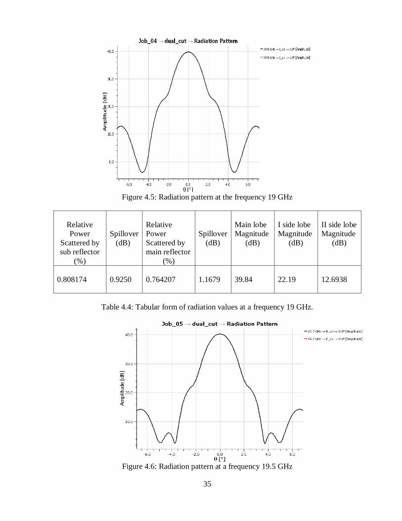
4.5 Radiation pattern at a frequency 19 GHz

35

4.6 Radiation pattern at a frequency 19.5 GHz

35

5.1 Gain vs. Number of iterations by using Iterative Local Search Algorithm

39

5.2 3-D View of the Cassegrain Reflector Antenna

39

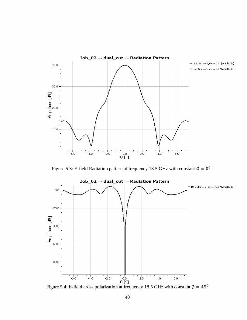
5.3 E-field Radiation pattern at frequency 18.5 GHz with constant ∅ = 00

40

5.4 E-field cross polarization at frequency 18.5 GHz with constant ∅ = 450

40

5.5 Far field ′∅′ constant magnitude cuts using ICARA

41

5.6 Near field ′∅′ constant magnitude cuts using ICARA

41

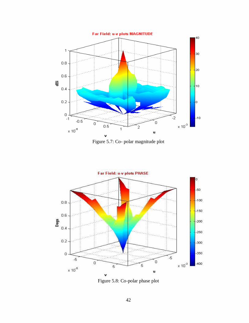
5.7 Co- polar magnitude plot

42

5.8 Co-polar phase plot

42

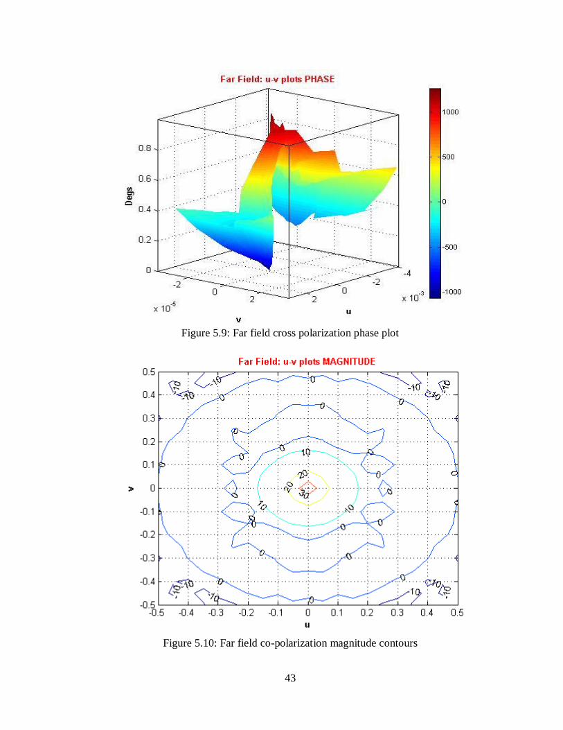
5.9 Far field cross polarization phase plot

43

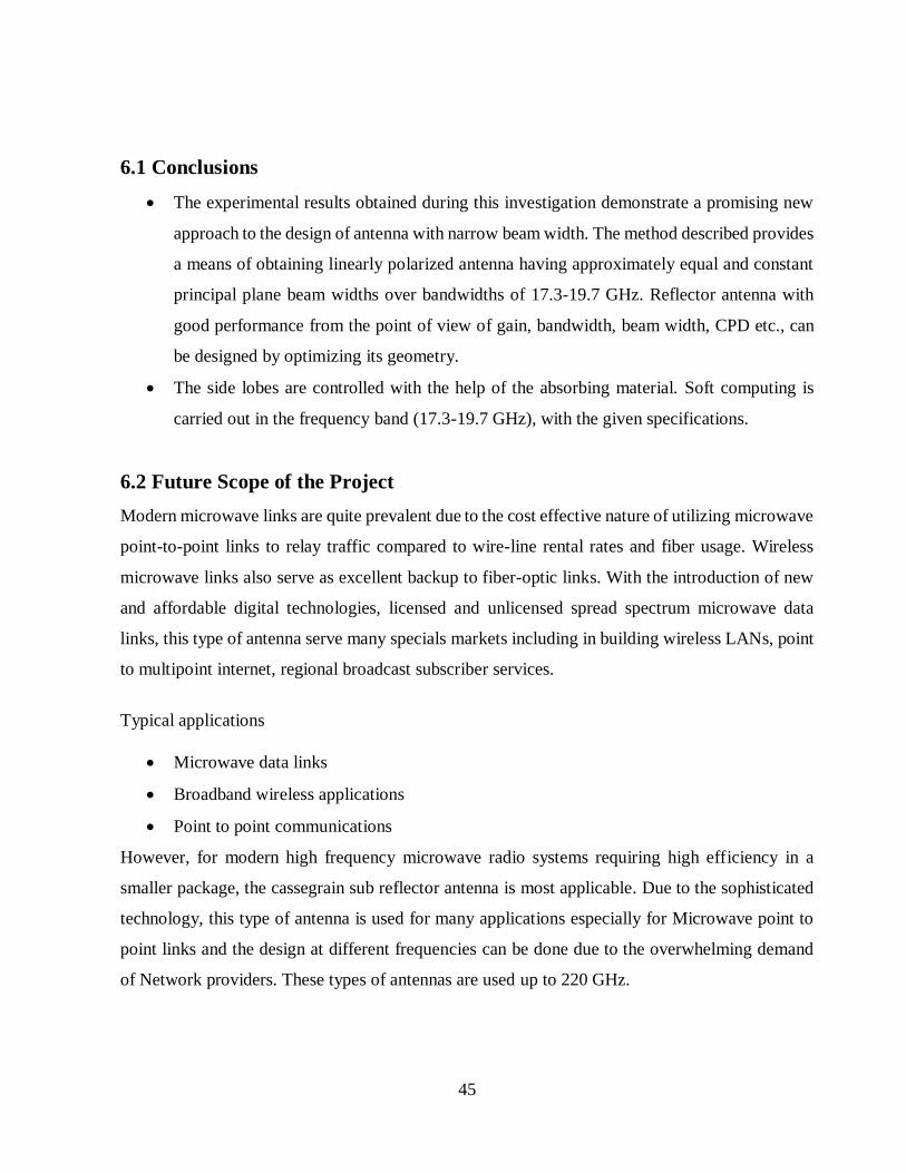
5.10 Far field co-polarization magnitude contours 43

viii

LIST OF TABLES

2.1 Main Reflector Contour Co-ordinates

21

2.2 Sub Reflector Contour Co-ordinates

23

4.1 Tabular form of radiation values at a frequency 17.3 GHz.

33

4.2 Tabular form of radiation values at a frequency 18 GHz.

33

4.3 Tabular form of radiation values at a frequency 18.5 GHz.

34

4.4 Tabular form of radiation values at a frequency 19 GHz.

35

4.5 Tabular form of radiation values at a frequency 19.7 GHz.

36

4.6 Tabular Form of beam width and gains with varying frequencies 36

1

CHAPTER 1

INTRODUCTION

AND

SCOPE OF THE PROJECT

2

1.1 Objective

Dual reflector antennas are considered as pencil beam antennas that can produce radiation

identical to searchlight beams. As compared with front-fed configuration, design of dual-reflector

geometry is complicated since the parameters like feed location, sub reflector size, required taper

on sub reflector, selection of focal length to diameter ratio of the main reflector, amplitude

distribution provided by feed etc. are to be adjusted as per the given specifications. Also the side

lobe suppression effort requires the antenna to be designed for minimum sub reflector blockage.

The design of such a cassegrain reflector is considered for the minimum blockage condition. Along

with the parameters like high gain and low cross-polarization; low VSWR is also one of the

prenominal parameter that can be achieved. The optimized values of 𝑓

𝐷 and angle subtended by

the sub reflector is obtained by using Iterative Local Search algorithm. For obtaining the radiation

diagrams, ‘Induced Current Analysis of Reflector Antenna’ and GRASP soft wares are used. This

will help us to identify the factors that affect the radiation pattern of the antenna.

1.2 Motivation

During the 1980s the need became greater for a lower profile microwave antenna that also

exhibited superior pattern performance. Two forces drove this requirement. One was the need to

reduce the visual impact of radio communication installations. The other was the need to place

more and more microwave links in the same geographic area. Large aperture antennas can be built

with reflectors or arrays but reflectors are far simpler than arrays. Array needs an elaborate network

but reflector uses simple feed and free space. At microwave frequencies the physical size of a high

gain antenna becomes small enough to make the practical use of suitably shaped reflectors to

produce the desired directivity. Here reflectors are curved surfaces. Although wire or rod antennas

can be and are used either singly or in arrays at UHF and SHF but other types utilizing reflecting

or radiating surfaces are generally more practical and hence used extensively. As the frequency

increases, the wavelength decreases and thus it becomes easier to construct an antenna system that

are large in terms of wavelengths and which therefore can be made to have greater directivity.

Parabolic reflectors are based on the geometric optical principles. Their feed

methods are also not by coaxial cable but by optical methods. Reflector antennas in one form or

another have been in use since the discovery of electromagnetic wave propagation in 1888 by

Hertz. The spectacular progress in the development of sophisticated analytical and experimental

techniques in shaping the reflector surfaces and optimizing illumination over their apertures so as

3

to maximize the gain lead to vital applications resulting in establishing the reflector antenna almost

as a household word during the 1960s.

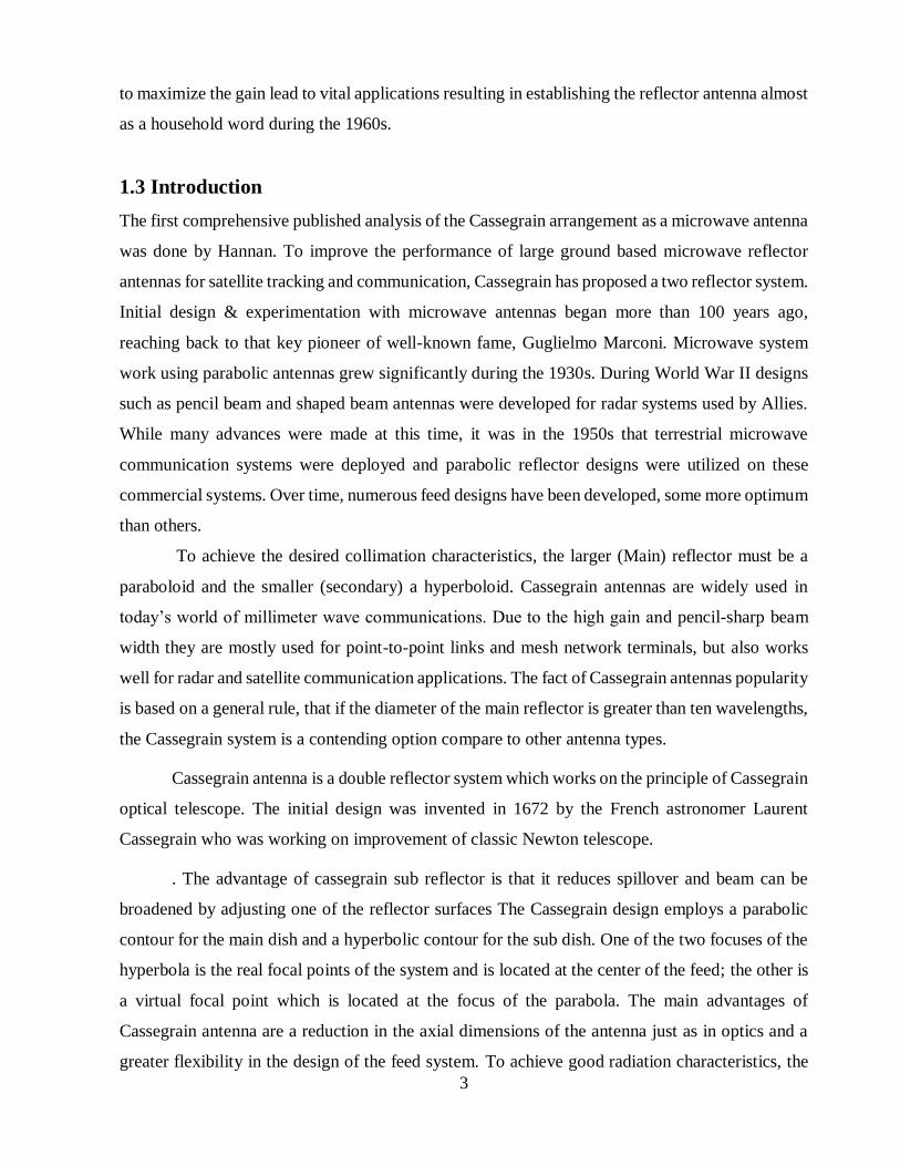
1.3 Introduction

The first comprehensive published analysis of the Cassegrain arrangement as a microwave antenna

was done by Hannan. To improve the performance of large ground based microwave reflector

antennas for satellite tracking and communication, Cassegrain has proposed a two reflector system.

Initial design & experimentation with microwave antennas began more than 100 years ago,

reaching back to that key pioneer of well-known fame, Guglielmo Marconi. Microwave system

work using parabolic antennas grew significantly during the 1930s. During World War II designs

such as pencil beam and shaped beam antennas were developed for radar systems used by Allies.

While many advances were made at this time, it was in the 1950s that terrestrial microwave

communication systems were deployed and parabolic reflector designs were utilized on these

commercial systems. Over time, numerous feed designs have been developed, some more optimum

than others.

To achieve the desired collimation characteristics, the larger (Main) reflector must be a

paraboloid and the smaller (secondary) a hyperboloid. Cassegrain antennas are widely used in

today’s world of millimeter wave communications. Due to the high gain and pencil-sharp beam

width they are mostly used for point-to-point links and mesh network terminals, but also works

well for radar and satellite communication applications. The fact of Cassegrain antennas popularity

is based on a general rule, that if the diameter of the main reflector is greater than ten wavelengths,

the Cassegrain system is a contending option compare to other antenna types.

Cassegrain antenna is a double reflector system which works on the principle of Cassegrain

optical telescope. The initial design was invented in 1672 by the French astronomer Laurent

Cassegrain who was working on improvement of classic Newton telescope.

. The advantage of cassegrain sub reflector is that it reduces spillover and beam can be

broadened by adjusting one of the reflector surfaces The Cassegrain design employs a parabolic

contour for the main dish and a hyperbolic contour for the sub dish. One of the two focuses of the

hyperbola is the real focal points of the system and is located at the center of the feed; the other is

a virtual focal point which is located at the focus of the parabola. The main advantages of

Cassegrain antenna are a reduction in the axial dimensions of the antenna just as in optics and a

greater flexibility in the design of the feed system. To achieve good radiation characteristics, the

4

sub reflector or sub dish must be a several, at least a few wavelengths in diameter and usually it is

ten times the main reflector size in wavelengths.

1.4 Specifications of 18.5 GHz Reflector Antenna

1.4.1 General

Antenna Type : High performance, low profile Cassegrain Reflector

Diameter : 635 mm

Polarization : Single Linear

Operative Frequency Range : (17.3 -19.7) GHz

1.4.2 Electrical

RPE(Radiation Pattern Envelope) : Class 2, ETSI (European Telecommunications Standards

Institute)

Minimum Gain : 38 dBi

MaximumXPD (Cross

Polarization Discrimination)

: 30 dB

Maximum VSWR (Voltage

Standing Wave Ratio)

: 1.3 : 1

Front to Back Ratio : 58 dB

1.5 Aim of the project

The aim of the project is to “Optimized Design of Axially Symmetric Cassegrain

Reflector Antenna using Iterative Local Search Algorithm”

A reflector antenna with a Cassegrain sub reflector can be used to obtain high gains. In

many professional applications this can be used for satellite as well as for astronomy, microwave

data links and other new emerging modes of personal and business communications. It is often

being seen on radio relay towers and mobile phone antenna masts.

5

1.6 Organization of Thesis

The following paragraphs summarize the content of each chapter.

Chapter-1 Gives an introduction and aim of the project

Chapter-2 Highlights the basic nature of Cassegrain Reflector antenna theory and gives the

step by step design approach.

Chapter-3 Gives the optimized values of variables using Iterative Local Search.

Chapter-4 Analysis of Cassegrain Antenna using GRASP software.

Chapter-5

Chapter-6

Results.

Gives the conclusion and the future scope of the project

6

CHAPTER 2

CASSEGRAIN ANTENNA

CONFIGURATION

7

2.1 Introduction

A typical parabolic antenna consists of a parabolic reflector with a small feed antenna at its focus.

The reflector is a metallic surface formed into a paraboloid of revolution and (usually) truncated

in a circular rim that forms the diameter of the antenna. This paraboloid possesses a distinct focal

point by virtue of having the reflective property of parabolas in that a point light source at this

focus produces a parallel light beam aligned with the axis of revolution. The feed antenna at the

reflector's focus is typically a low gain type such as a small waveguide horn. In more complex

designs, such as the cassegrain antenna, a sub-reflector is used to direct the energy into the

parabolic reflector from a feed antenna located away from the primary focal point. The feed

antenna is connected to the associated radio-frequency (RF) transmitting or receiving equipment

by means of coaxial cable transmission line or hollow waveguide .Sometimes it becomes important

to minimize the length of transmission line or waveguide connecting the feed radiator with receiver

or transmitter. This is needed specially to avoid losses. Although there could be a solution of this

problem by placing RF amplifier stage of receiver near the focus which minimizes the losses on

reception. But this is not practicable for transmission, as the RF amplifier of a transmitter is bulky,

heavy and having enough power so it is not possible to place at feed point. Hence the practical

solution in such case is cassegrain configuration when the transmission line or waveguide length

between feed and transmitter and receiver is required to be short.

2.1.1 Advantages

Spillover and minor lobe radiation is less.

It is possible to scan the beam or to broaden the beam by moving the reflecting surfaces.

High gain can be achieved

8

2.2 Cassegrain Antenna Design

Figure 2.1: 2-D CAD view of Cassegrain Antenna

2.2.1 Cassegrain Antenna Design Parameters

𝐷𝑝 = Parabolic dish diameter

𝑓𝑝 = Parabolic dish focal length

𝑑𝑠𝑢𝑏 = Sub reflector diameter

𝑓ℎ𝑦𝑝 = focal length of hyperbola – between foci

𝑎 = parameter of hyperbola

𝑐 =𝑓ℎ𝑦𝑝

2 = parameter of hyperbola

ø0 = angle subtended by parabola

𝜓= angle subtended by sub reflector

ø𝑏 = angle blocked by sub reflector

α = angle blocked by feed horn

9

2.3 Parabolic Reflector

A Parabola is a two dimensional plane wave. A practical reflector is a three dimensional

curved surface. Therefore, a practical reflector is formed by rotating a parabola about its axis. The

surface so generated is known as PARABOLOID which is often called as “MICROWAVE DISH”

or “PARABOLIC REFLECTOR”.

Parabolic produces a parallel beam of circular cross section because the mouth of the

parabola is circular. If a third Cartesian co-ordinate z has its axis perpendicular to both X axis and

Y axis.

𝑦2 + 𝑧2 = 4𝑓𝑥 …………………………….. (2.3.1)

Narrow major beam is in the direction of paraboloid axis. If the feed or primary antenna

is isotropic then the paraboloid will produce a beam of radiation. Assuming circular aperture is

large, the BWFN (Beam Width between First Nulls)

𝐵𝑊𝐹𝑁 =140𝜆

𝐷 …………………. …… (2.3.2)

Where

𝜆= free space wavelength in meters.

D= Diameter of aperture in meters.

For rectangular aperture,

𝐵𝑊𝐹𝑁 =115𝜆

𝐿 …………………. (2.3.3)

Where L = Length of aperture (λ)

Width between half power points for a large circular aperture is given by

𝐻𝑃𝐵𝑊 =58𝜆

𝐷 ………………. (2.3.4)

Further the directivity D of a large uniform illuminated aperture,

𝐷 =4𝜋𝐴

𝜆2 .............................. (2.3.5)

For circular aperture

𝐷 =4𝜋𝐴

𝜆2 …….. ……….. …….. ………… …… (2.3.6)

𝐷 = 9.87 (𝐷

𝜆)

2 ................. (2.3.7)

10

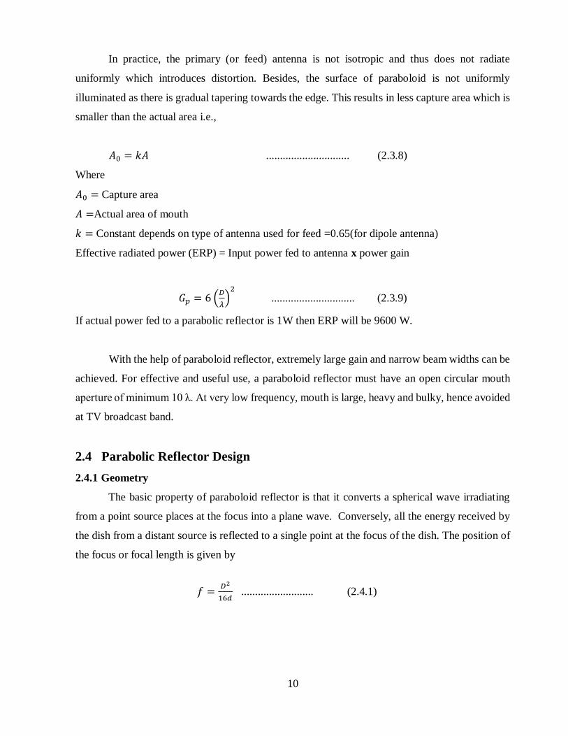
In practice, the primary (or feed) antenna is not isotropic and thus does not radiate

uniformly which introduces distortion. Besides, the surface of paraboloid is not uniformly

illuminated as there is gradual tapering towards the edge. This results in less capture area which is

smaller than the actual area i.e.,

𝐴0 = 𝑘𝐴 .............................. (2.3.8)

Where

𝐴0 = Capture area

𝐴 =Actual area of mouth

𝑘 = Constant depends on type of antenna used for feed =0.65(for dipole antenna)

Effective radiated power (ERP) = Input power fed to antenna x power gain

𝐺𝑝 = 6 (𝐷

𝜆)

2

.............................. (2.3.9)

If actual power fed to a parabolic reflector is 1W then ERP will be 9600 W.

With the help of paraboloid reflector, extremely large gain and narrow beam widths can be

achieved. For effective and useful use, a paraboloid reflector must have an open circular mouth

aperture of minimum 10 λ. At very low frequency, mouth is large, heavy and bulky, hence avoided

at TV broadcast band.

2.4 Parabolic Reflector Design

2.4.1 Geometry

The basic property of paraboloid reflector is that it converts a spherical wave irradiating

from a point source places at the focus into a plane wave. Conversely, all the energy received by

the dish from a distant source is reflected to a single point at the focus of the dish. The position of

the focus or focal length is given by

𝑓 =𝐷2

16𝑑 .......................... (2.4.1)

11

2.4.2 f/D Ratio

Paraboloid reflector can be designed by keeping the mouth diameter fixed and varying the

focal length(f) also .In designing a reflector antenna , the antenna needs to properly illuminate the

reflector i.e., the beam width of the antenna needs to match the f/D ratio of the parabolic reflector.

Otherwise the antenna of an over illuminated reflector would receive a noise from behind the

parabolic reflector. Likewise, an under illuminated reflector does not use its total surface area to

focus a signal on its antenna.

Size of the dish is the most important factor since it determines the maximum gain that can

be achieved at the given frequency and the resulting beam width.

Gain 𝐺 = (𝜋𝐷

𝜆)

2

∗ 𝜂 .............................. …………………………. (2.4.2)

Efficiency is determined mainly by the effectiveness of illumination of the dish by the feed. Each

time the diameter of a dish is doubled the gain is four times or 6 dB greater. The lower the f/d ratio,

the lower the side lobes because the feed is more protected from stray rays. Side lobes can also be

reduced by means of additional shielding on the rim of the parabolic reflector.

Half subtended angle of the main reflector ∅ = 2 𝑇𝑎𝑛−1 (1

4(𝑓

𝐷𝑝))………………….. … (2.4.3)

Effective focal length of the main reflector 𝑓𝑒 =𝐷

4 𝑇𝑎𝑛(𝛹

2) ……………………………... (2.4.4)

Space attenuation of the main reflector (𝑆. 𝐴)𝑀𝑎𝑖𝑛 = 20𝑙𝑜𝑔 (2

1+𝑐𝑜𝑠(∅))……………….. (2.4.5)

Optimum value of the illumination taper is given by the graph or formula

𝑡𝑎𝑝𝑒𝑟 = 0.72(𝑙𝑜𝑔𝐷𝑝)2

− 4.16(𝑙𝑜𝑔𝐷𝑝) + 17.7 When 𝐷𝑝 < 500𝜆… (2.4.6)

Milligan includes approximations for the losses in smaller dishes, based on the work of Kidal.

Diffraction is a major contributor to losses in small dishes. Kidal found that the illumination edge

taper in a Cassegrain antennas should be greater than the nominal 10 dB edge taper for prime focus

dish, to reduce diffraction loss. Since diffraction occurs near the edge of a reflector, reducing the

edge illumination should reduce the diffracted energy, while the illumination loss increases

slightly. The plot which gives the relation between optimum illumination taper vs. dish diameter

is

12

Figure 2.2: Cassegrain Antenna Edge Taper

Adjusted illumination taper of the feed w.r.t. sub reflector to get the desired taper is

𝜓1 = 𝜓√(𝑡𝑎𝑝𝑒𝑟 𝑖𝑛 𝑑𝐵−𝑆.𝐴𝐷𝑖𝑠ℎ

10−𝑆.𝐴𝑠𝑢𝑏) ………………………… (2.4.7)

Adjusted effective focal length 𝑓𝑒1 =

𝐷𝑝

4 𝑇𝑎𝑛(𝛹1

2) ……………………….. (2.4.8)

2.4.3 Electrical and Mechanical considerations for f/D Ratio

Small f/D ratio for deep-dish reflectors

Large f/D ratio for shallow dish reflectors

Shallow dishes are easier to support and move mechanically

Feed has to be farther from reflector

Farther feed results in narrow primary pattern

Feed has to be larger also

f/D ranges from 0.3-0.5 in general and 0.5 -1.0 for mono-pulse tracking radar antennas

13

Figure 2.3: CAD view of Parabolic Reflector Contour

2.5 Dish Illumination

Illuminate as much as the reflecting surface as possible as well as avoiding spillover. Best

results are obtained with a tapered illumination that will progressively diminish the illumination

of the edges thus reducing side lobes and spillover. Two dishes of the same diameter but different

focal lengths require different designs of feed if both are illuminated efficiently.

2.6 Advantages of Parabolic Reflectors

Parabolic reflectors can provide high gain.

Ease of fabrication in quantities.

Small gain antennas can be used ad feed to obtain high gain.

Complete transceiver can be located at the focus of a very cost effective long distance

communication system.

2.7 Shroud

Shrouds are added to parabolic microwave antennas to reduce the side lobe level being radiated to

reduce the side lobe level being radiated. They appear to look like drums or a tunnel that has a

diameter about the same as the parabolic reflector and is bolted on the surface. The shroud is also

lined with flat absorber material to enhance pattern performance.

14

2.8 Cassegrain SubReflector

The Cassegrain antenna adds a hyperbolic subreflector, acting as a mirror to reflect the feed

position back toward the main reflector. . To minimize loss from diffraction and spillover, the

subreflector should be electrically large, greater than 10 wavelengths in diameter, or about 1 foot

at 10 GHz. The subreflector diameter should be less than 20% of the dish diameter to minimize

blockage by the subreflector, so the dish should be larger than 50 wavelengths diameter. Antenna

efficiency decreasing rapidly for subreflectors smaller than ten wavelengths and for diameter ratios

greater than 0.1. For very deep dishes where available feeds can only provide poor efficiency, a

Cassegrain system with a good feed horn might achieve better overall efficiency. At the higher

microwave frequencies, feed line loss can be high enough to significantly reduce overall

efficiency, so the more accessible feed location of the Cassegrain system is a good alternative.

Hyperbola dimensions for the subreflector are necessary to reshape the feed horn pattern

to properly illuminate the dish, as well as the desired hyperbola focal length, the distance between

the two foci of the hyperbola. One focus of the hyperbola is at the focal point of the dish which is

called as the virtual focus. No RF ever reaches it, but the RF from the feed reflected by the

subreflector appears to originate from the virtual focus. The feed horn phase center is at the other

focus of the hyperbola. The feed horn illuminates the sub reflector, which subtends the angle𝛹.

Diffraction is a major contribution to losses in small dishes. Diffraction occurs near the edge of a

reflector, reducing the edge illumination should reduce the diffracted energy. The optimum sub

reflector size to minimize the combination of blockage and diffraction losses is given by

(𝑑𝑠𝑢𝑏

𝐷𝑝) = [

𝑐𝑜𝑠4(𝜓1

2) 𝐸 𝜆

(4𝜋)2 𝑠𝑖𝑛𝜙 𝐷𝑝]

15⁄

………………………. (2.8.1)

Where E is the edge taper

𝐸 = 10(−𝑡𝑎𝑝𝑒𝑟 𝑖𝑛 𝑑𝐵 10⁄ )

The optimum value of d/D, the ratio of subreflector diameter to dish diameter, for any

size dish and edge taper is given by the plot

15

Figure 2.4: Optimum Cassegrain Subreflector size

Approximate efficiency for the combination of blockage and diffraction losses,

𝜂𝑠𝑢𝑏 = [1 − 𝐶𝑏 (1 + 4 (1 − (𝑑𝑠𝑢𝑏

𝐷))

12⁄

) (𝑑𝑠𝑢𝑏

𝐷)]

2

…….. (2.8.2)

Where 𝐶𝑏 =−𝑙𝑛√(𝐸)

1−√(𝐸)

A feed horn with a wide beam would be closer to the sub reflector than a feed horn with a narrow

beam .The f/D for maximum efficiency is the dish best illuminated by that feed. The total edge

taper is the sum of the feed taper, radiation pattern of the feed at the edge of the dish, and the space

attenuation. For example, a dish with an f/D of 0.35 has 3.6 dB of space attenuation and an

illumination angle of 142 ° .To provide an edge taper of 10 dB, a feed must have a pattern that is

6.4 dB down at the edge, 90° from the axis, so that the sum of the pattern and the 3.6 dB space

attenuation is 10 dB Since the feed pattern is only 6.4 dB down at the edge, some spillover is

inevitable.

16

2.9 Feed Horn Design

A feed is the main point of contact between the dish and the coaxial cable or a waveguide. In short

feed is a medium of communication for the dish i.e., waves are transmitted and received with the

help of the dish. Horn is an impedance transformer, gradually transitioning from the constrained

impedance of a waveguide to the impedance of free space. A horn antenna is a useful and simple

radiator excited by waveguide. If the waveguide size is slowly expanded or tapered then more gain

can be achieved preventing undesired modes from reaching the waveguide. Horn antenna is used

as focal point feed in many reflector antennas. The losses in the horn are negligible. The function

of the horn is to produce a uniform phase front with a larger aperture than that of the guide and

hence greater directivity.

2.9.1 Waveguide Horn

More Directivity

Acts as point source with large reflectors

For uniform radiation pattern across parabolic aperture only a small angular portion of the

pattern should be used

The ratio of f/D should be large for uniform illumination

A part of energy radiated by the feed and not intercepted by the paraboloid amounts to loss.

This loss or spillover results in lowering the overall efficiency and defeats the purpose of

uniform illumination.

If the ratio f/D is increased further, spillover is less, intercepted energy and thus efficiency

increases. But since illumination is more tapered the aperture efficiency decreases.

Corrugated horn was described by Simmons and Kay and it is called as Scalar Feed. The

aperture diameter plus the length completely defines the horn. Corrugated horns exhibit a

combination of highly desirable characteristics such as high beam symmetry, low cross

polarization, low level of side lobes, good return loss and low attenuation.

The idea is to eliminate the E plane edge currents in the rim of the horn by adding slots or

grooves perpendicular to the length of the horn .The grooves are made deep enough so that the

surface reactance is capacitive, surface waves cannot be supported. The required depth is greater

than λ/4.

Conical horns are simpler. The aperture diameter is chosen analytically to give the desired

co-planar pattern beam width. For the linear design, the diameter has been evaluated by means of

17

simulations carried out by calculating the radiation pattern under the pure HE11 mode propagation

in circular waveguide with a phase distribution given by a spherical phase front with center in the

apex of the horn. Since the depth and shape of corrugations determine the cross-polarization

radiation characteristic, their geometry was selected to give the minimum level of cross-

polarization at the center frequency.

The corrugations are about a quarter wavelengths deep and there are at least three corrugations per

wavelength in order to well approximate a continuous impedance surface. The junction and throat

region were designed to optimize the impedance match to the smooth wall waveguide. For this

purpose the first slot seen but the smooth wall waveguide is approximately half a wavelength deep

with the following few slots (about 5) constituting a transition region to the quarter wavelength

steady state depth of the remaining part.. Also the teeth and groove length need to be varied

continuously between the first corrugations and the steady state region; a good input matching

require thick teeth and thin grooves which are used at the beginning, while on the contrary , HE11

propagation is well supported by thick grooves and thin teeth.

One focus of the hyperbola is at the focal point of the dish; which is referred to as virtual

focus. No RF ever reaches it, but the RF from the feed reflected by the sub reflector appears to

originate from the virtual focus. The feed horn phase center is at the other focus of the hyperbola.

The feed horn illuminates the sub reflector, which subtends the angle ψ. A feed horn with

a wide beam would be closer to the sub reflector than a feed horn with a narrow beam.

The subtended half-angle to illuminate a given f/D is

𝜓 = 2 𝑇𝑎𝑛−1 (1

4(𝑓

𝐷)) ………………. (2.9.1)

To adjust this for the edge taper, we use Kelleher's universal horn equation to correct the

illumination angle for the desired edge taper.

𝜓1 = 𝜓√(𝑡𝑎𝑝𝑒𝑟 𝑖𝑛 𝑑𝐵

10)………………. (2.9.2)

The adjusted illumination angle for desired taper can be calculated from feed horn

𝜓1 = 𝜓√(𝑡𝑎𝑝𝑒𝑟 𝑖𝑛 𝑑𝐵−𝑆.𝐴𝐷𝑖𝑠ℎ

10−𝑆.𝐴𝑠𝑢𝑏) …………………….. (2.9.3)

The feed must be positioned such that the angle subtended by the sub reflector is ψ`, placing the

feed at one focus of the hyperbola and the dish prime focus at the other as shown in Fig 2.1.

Thus, the hyperbola focal length, the distance between the two foci is

18

𝑓ℎ𝑦𝑝 = 0.5𝑑𝑠𝑢𝑏(𝑐𝑜𝑡(𝜓1) + 𝑐𝑜𝑡(𝜓))……………… (2.9.4)

Rays near the center of the beam that reflect from the sub reflector at angles less than 𝜑𝑏 are

eventually blocked by the sub reflector. If 𝛼 > 𝜑𝑏 then the angle shadowed by the feed horn is

larger than the angle shadowed by the sub reflector, so the feed will cause additional blockage loss.

𝜑𝑏 = 𝑠𝑖𝑛−1 (𝑑𝑠𝑢𝑏

2𝑓𝑝) ……………………. (2.9.5)

𝛼 = 𝑇𝑎𝑛−1 (𝑑𝑓𝑒𝑒𝑑

2𝑓ℎ𝑦𝑝) …………………......…. (2.9.6)

The effective 𝑓

𝐷⁄ for the feed is given by

𝐸𝑓𝑓𝑒𝑐𝑡𝑖𝑣𝑒 𝐹𝑒𝑒𝑑 𝑓

𝐷⁄ =1

4𝑇𝑎𝑛(𝜓

2) ………….. (2.9.7)

The sub reflector must reshape the illumination from the effective feed 𝑓

𝐷 to

𝑓𝑝

𝐷𝑝 for the dish

The magnification factor is given by

𝑀 =𝐸𝑓𝑓𝑒𝑐𝑡𝑖𝑣𝑒 𝐹𝑒𝑒𝑑 (

𝑓

𝐷)

(𝑓𝑝

𝐷𝑝)

……………………. (2.9.8)

The amount of curvature is called Eccentricity,

Eccentricity 𝑒 =𝑀+1

𝑀−1 …………………. (2.9.9)

Hyperbola parameters can be calculated as

𝑐 =𝑓ℎ𝑦𝑝

2 ……………… (2.9.10)

𝑎 =𝑐

𝑒 ………………… (2.9.11)

𝑏 = √(𝑐2 − 𝑎2) …………. (2.9.12)

The distance from the apex of the apex of the sub reflector to the virtual focus (focus of the main

parabola) behind the sub reflector is 𝑐 − 𝑎.

The distance from the apex of the sub reflector to the phase center of the feed horn is 𝑐 + 𝑎.

To eliminate feed horn blockage, the feed horn must be moved farther away from the sub reflector.

There are two ways to move the feed horn without upsetting the geometry. One choice is a feed

horn with a narrower beam, reducing angle 𝜓 (recalculate𝑓ℎ𝑦𝑝); narrower beams require larger

horn apertures. The other choice is a larger sub reflector, which increases the focal distance without

changing angle 𝜓. This will increase blockage loss only, so the efficiency will

decreases slightly and should be recalculated. The minimum sub reflector diameter to avoid feed

horn blockage is

19

𝑑𝑠𝑢𝑏 > 𝑑𝑓𝑒𝑒𝑑 (𝑓𝑝

𝑓ℎ𝑦𝑝) ………………….. (2.9.13)

The sub reflector must be in the far field of the feed horn which can be checked by Rayleigh

Distance,

𝑐 + 𝑎 > 2 (𝑑𝑓𝑒𝑒𝑑

2

𝜆)……………… (2.9.14)

If the sub reflector is in the near field of the feed, there will be significant phase error. The error

decreases as the spacing approaches the Rayleigh Distance.

2.10 Radome

A radome is a structural, weatherproof enclosure that protects a microwave or radar

antenna. The radome is constructed of material that minimally attenuates the electromagnetic

signal transmitted or received by the antenna.

In other words, the radome is transparent to radar or radio waves. Radomes protect the

antenna surfaces from the environment (e.g., wind, rain, ice, sand, ultraviolet rays etc.) and or

conceal antenna electronic equipment from public view. They also protect nearby personnel from

being accidentally struck by quickly-rotating antennas.

Radomes can be constructed in several shapes (spherical, geodesic, planar, etc.) depending

upon the particular application using various construction materials (fiberglass, PTFE -coated

fabric, etc.). When used on UAVs or other aircraft in addition to such protection, the radome also

streamlines the antenna system, thus reducing drag. A radome is often used to prevent ice and

freezing rain from accumulating directly onto the metal surface of the antennas as in the case of a

spinning radar dish antenna. The radome also protects the antenna from debris and rotational

irregularities due to wind.

For stationary antennas, excessive amounts of ice can de-tune the antenna to the point

where its impedance at the input frequency rises drastically, causing voltage standing wave ratio

(VSWR) to rise as well. This reflected power goes back to the transmitter, where it can cause

overheating. A fold back circuit can act to prevent this; however, one drawback of its use is that it

causes the station's output power to drop dramatically, reducing its range.

A radome prevents that by covering the antenna's exposed parts with a sturdy, weatherproof

material, typically fiberglass, which keeps debris or ice away from the antenna to prevent any

20

serious issues. It is interesting to note that one of the main driving forces behind the development

of fiberglass as a structural material was the need during World War II for radomes. When

considering structural load, the use of a radome greatly reduces wind load in both normal and iced

conditions. Many tower sites require or prefer the use of radomes for wind loading benefits and

for protection from falling ice or debris.

2.11 18.5 GHz Main Reflector Design Values

Frequency band: K- band

Operative Frequency range: (17.3 − 19.7) 𝐺𝐻𝑧

Centre Frequency 𝐹𝑐 =𝐹𝐻+𝐹𝐿

2=

(17.3+19.7)

2= 18.5 𝐺𝐻𝑧

Diameter : 𝐷 = 635 𝑚𝑚 𝑓

𝐷=0.3995

Focal length of the Main Reflector 𝑓 = 253.6825 𝑚𝑚

Wavelength 𝜆 =𝐶

𝐹𝑐=

300

18.5= 16.216 𝑚𝑚

Depth of Dish, 𝑑 =𝐷2

16𝑓= 99.3429 𝑚𝑚

𝐴 = physical area of the reflector

𝐴 =𝜋𝐷2

4= 316692 𝑚𝑚2

𝜂 = aperture efficiency /illumination efficiency

Gain 𝐺 = 10𝑙𝑜𝑔 ∗ 𝜂 ∗ (4𝜋𝐴

𝜆2 ) = 41.799 𝑑𝐵

Parabola equation 𝑦2 = 4𝑓𝑥

Then 𝑥 =𝑦2

4𝑓

21

2.12 Main Reflector Contour Co-ordinates

Y (mm) X (mm)

25 0.6159

50 2.4637

75 5.5433

100 9.8548

125 15.398

150 22.173

175 30.180

200 39.419

225 49.890

250 61.592

275 74.527

300 88.693

317.5 99.342

Table 2.1: Main Reflector Contour Co-ordinates

2.13 18 GHz Cassegrain Sub Reflector Design

Design Values

𝐷𝑝 = Parabolic Dish diameter = 635mm

𝑓𝑝 = Parabolic Dish Focal Length = 253.6825 𝑚𝑚

𝑓

𝐷 Of Main Dish = 0.3995

Sub Reflector Geometry

Magnification Factor 𝑀 =𝐸𝑓𝑓𝑒𝑐𝑡𝑖𝑣𝑒 𝐹𝑒𝑒𝑑 (

𝑓

𝐷)

(𝑓𝑝

𝐷𝑝)

= 4.7494

𝑑𝑠𝑢𝑏 = Sub Reflector Diameter = 66.0123 𝑚𝑚

𝑓ℎ𝑦𝑝 = Focal length of hyperbola between foci = 141.6341 𝑚𝑚

Dish illumination Half Angle 𝜓 = 2 𝑇𝑎𝑛−1 (1

4(𝑓

𝐷)) = 64.0752

Angle blocked by sub reflector 𝜑𝑏 = 𝑠𝑖𝑛−1 (𝑑𝑠𝑢𝑏

2𝑓𝑝)

Angle blocked by feed horn 𝛼 = 𝑇𝑎𝑛−1 (𝑑𝑓𝑒𝑒𝑑

2𝑓ℎ𝑦𝑝)

22

Hyperbola Parameters :

𝑎 = 46.1824 𝑚𝑚 𝑏 = 53.6865 𝑚𝑚 𝑐 = 70.8171 𝑚𝑚

Eccentricity

𝑒 =𝑀 + 1

𝑀 − 1= 1.5334

𝑐 =𝑓ℎ𝑦𝑝

2= 70.8171 𝑚𝑚

𝑎 =𝑐

𝑒= 46.1824 𝑚𝑚

Space Attenuation of Parabolic Dish

(𝑆. 𝐴)𝐷𝑖𝑠ℎ = 20 ∗ 𝑙𝑜𝑔 (2

1+𝑐𝑜𝑠(𝜓)) = 2.8703 𝑑𝐵

Space Attenuation of Feed

(𝑆. 𝐴)𝑠𝑢𝑏 = 20 ∗ 𝑙𝑜𝑔 (2

1+𝑐𝑜𝑠(𝜃)) = 0.1495 𝑑𝐵

Adjusted illumination angle to get the desired taper 𝜓1 = 𝜓√(𝑡𝑎𝑝𝑒𝑟 𝑖𝑛 𝑑𝐵−𝑆.𝐴𝐷𝑖𝑠ℎ

10−𝑆.𝐴𝑠𝑢𝑏) = 60.6522

Keheller’s Universal Horn Equation, 𝜓1 = 𝜓√𝑇𝑎𝑝𝑒𝑟 𝑖𝑛 𝑑𝐵

Edge Taper 𝐸 = 10(𝑇𝑎𝑝𝑒𝑟 𝑖𝑛 𝑑𝐵

10) = 0.0677

Approximate Sub-Reflector Efficiency

𝜂𝑠𝑢𝑏 = [1 − 𝐶𝑏 (1 + 4 (1 − (𝑑𝑠𝑢𝑏

𝐷))

12⁄

) (𝑑𝑠𝑢𝑏

𝐷)]

2

= 0.8206

𝐶𝑏 =−𝑙𝑛√(𝐸)

1 − √(𝐸)

Minimum Sub Reflector Diameter to avoid feed horn blockage = 66.0123 𝑚𝑚

Sub Reflector Position:

Apex to Dish Focal point = 24.6347 𝑚𝑚

Apex to Feed Phase Center = 1116.9995 𝑚𝑚

Equation of the Hyperbola is 𝑥2

𝑎2−

𝑦2

𝑏2= 1

Then 𝑥 = √𝑎2 (1 +𝑦2

𝑏2)

23

2.14 Sub Reflector Contour Co-ordinates

Radius Y (mm) X (mm)

0 8.86

4.01 7.84

8.05 7.77

12.08 7.38

16.11 6.91

20.13 6.44

24.17 5.97

28.20 5.50

32.23 4.98

Table 2.2: Sub Reflector Contour Co-ordinates

2.15 Summary

This chapter concludes with the design of main reflector, sub reflector and feed horn with

relevant procedure and calculations.

24

CHAPTER 3

ITERATIVE LOCAL SEARCH

ALGORITHM

25

3.1 Iterated Local Search algorithm

Iterated Local Search is a Met heuristic and Global Optimization technique. It is an extension of

Multi Start Search and may be considered a parent of many two-phase search approaches such as

the Greedy Randomized Adaptive Procedure and Variable Neighborhood Search.

3.1.1 Strategy

The objective of Iterated Local Search is to improve upon stochastic Multi-Restart Search by

sampling in the broader neighborhood of candidate solutions and using a Local Search technique

to refine solutions to their local optima. Iterated Local Search explores a sequence of solut ions

created as perturbations of the current best solution, the result of which is refined using an

embedded heuristic.

3.1.2 Pseudo code for Iterated Local Search.

Input:

Output: 𝑆𝑏𝑒𝑠𝑡

𝑆𝑏𝑒𝑠𝑡← Construct Initial Solution ();

𝑆𝑏𝑒𝑠𝑡← Local Search ();

Search History ←𝑆𝑏𝑒𝑠𝑡;

While ¬ Stop Condition () do

𝑆𝑐𝑎𝑛𝑑𝑖𝑑𝑎𝑡𝑒← Perturbation (𝑆𝑏𝑒𝑠𝑡, SearchHistory);

𝑆𝑐𝑎𝑛𝑑𝑖𝑑𝑎𝑡𝑒← Local Search (𝑆𝑐𝑎𝑛𝑑𝑖𝑑𝑎𝑡𝑒);

Search History ←𝑆𝑐𝑎𝑛𝑑𝑖𝑑𝑎𝑡𝑒 ;

If Acceptance Criterion (𝑆𝑏𝑒𝑠𝑡,𝑆𝑐𝑎𝑛𝑑𝑖𝑑𝑎𝑡𝑒 SearchHistory) then

𝑆𝑏𝑒𝑠𝑡← 𝑆𝑐𝑎𝑛𝑑𝑖𝑑𝑎𝑡𝑒 ;

End

End

Return 𝑆𝑏𝑒𝑠𝑡;

26

3.1.3 Heuristics

Iterated Local Search was designed for and has been predominately applied to discrete

domains such as combinatorial optimization problems.

The perturbation of the current best solution should be in a neighbor-hood beyond the

reach of the embedded heuristic and should not be easily undone.

Perturbations that are too small make the algorithm too greedy, perturbations that are too

large make the algorithm too stochastic.

The embedded heuristic is most commonly a problem-specific local search technique.

The starting point for the search may be a randomly constructed candidate solution, or

constructed using a problem-specific heuristic (such as nearest neighbor).

Perturbations can be made deterministically, although stochastic and probabilistic

(adaptive based on history) are the most common.

The procedure may store as much or as little history as needed to be used during

perturbation and acceptance criteria. No history represents a random walk in a larger

neighborhood of the best solution and is the most common implementation of the approach.

The simplest and most common acceptance criteria are an improvement in the cost of

constructed candidate solutions.

27

CHAPTER 4

ANALYSIS OF CASSEGRAIN ANTENNA

USING GRASP SOFTWARE

28

GRASP 10

(GENERAL REFLECTOR ARRAY SOFTWARE PACKAGE)

4.1 Introduction

The radiation of the whole antenna system is analyzed with TICRA’s GRASP software. It

uses both physical optics (PO) and geometric optics (GO) to compute reflection from surfaces that

are electrically large, i.e., at least several wavelengths in some dimension. Both PO and GO

methods are very computationally efficient, thus very large systems can be analyzed. For example,

single reflector systems that are several tens of wavelengths in size are analyzed within a few

minutes using an ordinary personal computer.

Radiation from the equivalent or induced surface currents on a reflector is quite straight

forward to calculate. However, determining these currents exactly (e.g., using Method of

Moments) is computationally very laborious if the surface is electrically large. In that case induced

currents can be approximated using the much simpler PO method. In the PO approximation it is

assumed that the surface current on an infinite planar surface being tangential to the scattering

surface at that point.

However, this assumption is not valid on the surface edges , and infinite half plane wave

models is used there to produce physical theory of diffraction (PTD) currents Combining PO and

PTD yields to very accurate results if a sufficiently dense integration grid for radiation integrals is

used. After calculating the scattered field from the reflector, the total radiated field is obtained by

adding incident field from the feed.

A GRASP simulation can include multiple reflectors and multiple feeds. Any second

degree surface can be defined as a reflector with arbitrary rim shape; however most common

reflectors and rims are included as predefined models.

In order to obtain a full radiation pattern, both PO and GO need to be used. If accurate

results far from the main beam are needed, PO becomes inefficient due to an extremely large

integration grid while GO is still efficient. As a rule of thumb, PO is used within and near the main

beam, whereas GO is need elsewhere.

GRASP 10 is a set of tools for analyzing general reflector antennas and antenna

farms. It contains three main components:

29

1. A pre-processor which assists the user in setting up the antenna geometry, in specifying the type

of analysis to be performed and in visualizing the system. In addition the pre- processor provides

a plotting facility for simple 2D-plots of pattern cuts and contours.

2. An analysis module which performs the electromagnetic analysis and calculates data used for

visualization.

3. A post-processor containing several data-processing and plotting facilities for calculated

patterns. Plots can be in the form of pattern cuts or in the form of contour plots in various

projections.

The electromagnetic methods which may be applied for the analysis are

Physical Optics (PO) with Physical Theory of Diffraction (PTD)

Geometrical Optics (GO) and Geometrical Theory of Diffraction (GTD)

Spherical Wave Expansion (SWE)

Plane Wave Expansion (PWE)

Methods of Moments (MoM)

It contains four tabs for analysis of the reflector system

1. Objects: In which the geometry of the antenna as well as the methods of calculation are

defined.

2. Command: In which commands for the analysis are given

3. Jobs: In which the analysis is started and previous analyses may be reviewed.

4. Results: In which the results of the analysis are shown.

4.2 Dual Reflector with Blockage

In this we are designing rotationally symmetric dual reflector antenna system. In such this the

blockage due to the sub reflector must be accurately modeled, since this can have significant

influence on the gain and side lobes. Moreover, the spillover from the feed must be included in

the computations because it can significantly contribute to the radiation pattern.

With the purpose of making the sub reflector blockage and feed spillover effects easily

perceived, the dimensions of the antenna are exaggerated relative to the traditional design.

Areal dual reflector would of course need some sort of support for the sub reflector, but

this is here neglected.

30

GRASP 10 Simulation involves

• Navigating in the pre-processor windows

• Defining the geometry of standard, double reflector systems

• Getting an overview of the objects and commands created

• Performing a PO-analysis of the reflector system

• Viewing the calculated radiation pattern

4.3 Subreflector Blockage

Another contribution that needs to be considered is the subreflector blocking the nominal field

from the main reflector. There are two approaches for this analysis:

1. The main reflector area behind the subreflector, hence, the area invisible from the boresight

direction, is replaced by a hole, i.e. the currents in this area shall not contribute to the field.

This is a fast approach but only close to boresight.

2. The current on the subreflector generated by letting the main reflector field illuminated the

subreflector are calculated. The fields from these currents are added to the far field. This

approach is accurate but time consuming relative to the first approach.

4.4 Visualizing the geometry

GRASP 10 contains two different ways of visualizing 3D-data for the system geometry. The

OpenGL Plot, where the plotting is performed using the OpenGL graphics library to generate plots

where the geometry is shown as wire-grids or solid surfaces. The Object Plot, where the plots are

shown as wire grids.

Select Command list then we get a dialog box click submit. Clicking the submit button now

launches the analysis module. Two browser windows prompts the user to give the names of an

output file and a log file. Following these definitions the analysis is launched. The progress of the

analysis is displayed in a command window as shown in Figure 3.9.The analysis is completed

when the message Press Enter to Continue is shown in the command line window. Press Enter to

close the window. The result of the analysis is a field calculation in two cuts in the far field .The

result is stored in the file named sph_1cut.We can now plot the result in GRASP 10 by clicking

Commands ►Plot commands.

31

4.4.1 Visualizing the Geometry as an OpenGL Plot

A useful way of viewing the geometry is to use the OpenGL plots available in GRASP 10. The

plotting is performed using the OpenGL graphics library. It is possible to rotate, translate and zoom

the geometry using a combination of keystrokes and mouse movements.

To visualize the geometry as an OpenGL plot

In the main menu, click Commands. ► Plot Commands ► OpenGL, all objects. The OpenGL plot

of objects window opens with a plot of the reflector configuration. The reflector and feed horn are

shown in grey which can be seen in Fig 3.10. The red, green and blue lines illustrate the x-, y- and

z-axes of the coordinate systems defined.

It is possible to:

• Rotate the configuration by dragging the mouse

• Zoom by holding the Shift-key and dragging the mouse up (zoom in) or down (zoom out)

• Translate the configuration by holding the Ctrl-key and dragging the mouse

Figure 4.1: Open GL Plot

Using OpenGL in the pre-processor, the geometry is plotted as seen from an observer close to the

reflector system. As a consequence, it is not possible to visualize a projection of the geometry onto

a plane, e.g. one of the coordinate planes. This can be accomplished using the Object Plot in the

pre-processor.

32

4.4.2 Visualizing the Geometry as an Object Plot

In the Object Plot the 3D geometry is plotted as seen from an observer infinitely far from the

reflector system. Hence, this visualization yields projections of the geometry.

To plot the geometry as an object plot

In the main menu, click Commands. ► Plot Commands ► Plot all objects. The Object plot

window opens with a plot of the reflector configuration. There is no limit on the number of Object

plot windows, which can be opened at a given time.

4.4.3 Radiation Pattern

The GRASP 10 objects define the geometry, the electromagnetic sources and the way to analyze

the reflector system. However, we need to specify which electromagnetic computation should be

carried out and in which order. This is done using the GRASP10 Commands. The Command list

shows a list of commands to be executed by the analysis module. The commands are executed

sequentially in the order specified in the Command list. To open the command list. In the main

menu bar, click Commands. ► Command list ► Plot 2D cut. This opens the Plot 2D cut window.

Click File ►Open to select the sph_1.cut.

The radiation patterns at different frequencies are observed i.e., at 17.3 GHz, 18 GHz,18.5 GHz,

19 GHz and 19.7 GHz as shown in Fig , Fig 3.17,Fig 3.19 and Fig 3.20.

Figure 4.2: Radiation pattern at a frequency 17.3 GHz

33

Relative

Power

Scattered by

sub reflector

(%)

Spillover

(dB)

Relative

Power

Scattered by

main reflector

(%)

Spillover

(dB)

Main lobe

Magnitude

(dB)

I side lobe

Magnitude

(dB)

II side lobe

Magnitude

(dB)

0.7818

1.0689

0.7350

1.3368

38.6273

15.2232

15.4420

Table 4.1: Tabular form of radiation values at a frequency 17.3 GHz.

Figure 4.3: Radiation pattern at a frequency 18 GHz

Relative

Power

Scattered by

sub reflector

(%)

Spillover

(dB)

Relative

Power

Scattered by

main reflector

(%)

Spillover

(dB)

Main lobe

Magnitude

(dB)

I side lobe

Magnitude

(dB)

II side lobe

Magnitude

(dB)

0.793483

1.004

0.745871

1.2734

38.8184

17.86

15.83

Table 4.2: Tabular form of radiation values at a frequency 18 GHz.

34

Figure 4.4: Radiation pattern at a frequency 18.5 GHz

Relative

Power

Scattered by

sub reflector

(%)

Spillover

(dB)

Relative

Power

Scattered by

main reflector

(%)

Spillover

(dB)

Main lobe

Magnitude

(dB)

I side lobe

Magnitude

(dB)

II side lobe

Magnitude

(dB)

0.813007

0.8991

0.771328

1.276

39.8779

7.4245

13.9346

Table 4.3: Tabular form of radiation values at a frequency 18.5 GHz.

35

Figure 4.5: Radiation pattern at the frequency 19 GHz

Relative

Power

Scattered by

sub reflector

(%)

Spillover

(dB)

Relative

Power

Scattered by

main reflector

(%)

Spillover

(dB)

Main lobe

Magnitude

(dB)

I side lobe

Magnitude

(dB)

II side lobe

Magnitude

(dB)

0.808174

0.9250

0.764207

1.1679

39.84

22.19

12.6938

Table 4.4: Tabular form of radiation values at a frequency 19 GHz.

Figure 4.6: Radiation pattern at a frequency 19.5 GHz

36

Relative

Power

Scattered by

sub reflector

(%)

Spillover

(dB)

Relative

Power

Scattered by

main reflector

(%)

Spillover

(dB)

Main lobe

Magnitude

(dB)

I side lobe

Magnitude

(dB)

II side lobe

Magnitude

(dB)

0.817258

0.8764

0.7775

1.0929

40.3962

21.1978

6.0154

Table 4.5: Tabular form of radiation values at the frequency 19.5 GHz.

Frequency

(GHz)

3 dB Beam

width (°)

Gain

(dBi)

17.3 1.7 38.62

18 1.6 38.82

18.5 1.6 39.88

19 1.7 39.84

19.7 1.8 40.39

Table 4.6: Tabular Form of beam width and gains with varying frequencies

4.5 Summary

GRASP simulation software is used and Gain versus Frequency, 2D-radiation pattern, side lobe

level, Beam width are calculated at a frequency band (17.3 GHz -19.7 GHz).

Different materials used for fabrication of Cassegrain Reflector antenna and their advantages are

4.6 Aluminum alloys

Advantages

• Good mechanical behavior.

• Light Weight

• Good corrosion resistance.

• Low wind pressure

• Easy to fabricate and assemble

• Ability to conform to different shapes

37

4.7 RF Absorber

Advantages

• Light weight

• Flexible

• Flat sheet broad band absorber

• Electrically conductive

• Reticulated open cell polyurethane foam sheet with a controlled conductivity gradient

carbon loading system

• Frequency range from 8-26.5 GHz

The final additional component that is added to create a high performance microwave antenna is

the Radome. The radome serves two purposes. One is to protect the inside of the antenna from the

elements. The second purpose is to reduce what would otherwise be significant wind loading on

the antenna due to the shroud catching if not for the radome. The Radome is made up of Forex

material and the radome is fixed by using plastic rivets.

High performance antennas are characterized by low VSWR, high efficiency feed horn and by a

tight profile tolerance of the reflector. All High performance antennas are equipped with plane

flexible radomes mounted on cylindrical shields whose internal surfaces are covered with

absorbing material in order to minimize the spillover loss and hence wide angle and back lobes.

High performance antennas are installed in very crowded microwave networks where the use of

antennas are characterized by the peculiarity of exceptionally good values of cross-polarization

discrimination in a solid angle centered around the antenna axis.

Among the innovative and conventional foundry processes for aluminum alloys, low

pressure die casting is characterized by several advantages including high yield excellent control

of operative parameters. This type of antenna is used in microwave point to point links and it

makes the transmission easy by avoiding cables.

38

5. RESULTS

39

Figure 5.1: Gain vs. Number of iterations by using Iterative Local Search Algorithm

Figure 5.2: 3-D View of the Cassegrain Reflector Antenna

40

Figure 5.3: E-field Radiation pattern at frequency 18.5 GHz with constant ∅ = 00

Figure 5.4: E-field cross polarization at frequency 18.5 GHz with constant ∅ = 450

41

Figure 5.5: Far field ′∅′ constant magnitude cuts using ICARA

Figure 5.6: Near field ′∅′ constant magnitude cuts using ICARA

42

Figure 5.7: Co- polar magnitude plot

Figure 5.8: Co-polar phase plot

43

Figure 5.9: Far field cross polarization phase plot

Figure 5.10: Far field co-polarization magnitude contours

44

CHAPTER 6

CONCLUSION

&

FUTURE SCOPE

45

6.1 Conclusions

The experimental results obtained during this investigation demonstrate a promising new

approach to the design of antenna with narrow beam width. The method described provides

a means of obtaining linearly polarized antenna having approximately equal and constant

principal plane beam widths over bandwidths of 17.3-19.7 GHz. Reflector antenna with

good performance from the point of view of gain, bandwidth, beam width, CPD etc., can

be designed by optimizing its geometry.

The side lobes are controlled with the help of the absorbing material. Soft computing is

carried out in the frequency band (17.3-19.7 GHz), with the given specifications.

6.2 Future Scope of the Project

Modern microwave links are quite prevalent due to the cost effective nature of utilizing microwave

point-to-point links to relay traffic compared to wire-line rental rates and fiber usage. Wireless

microwave links also serve as excellent backup to fiber-optic links. With the introduction of new

and affordable digital technologies, licensed and unlicensed spread spectrum microwave data

links, this type of antenna serve many specials markets including in building wireless LANs, point

to multipoint internet, regional broadcast subscriber services.

Typical applications

Microwave data links

Broadband wireless applications

Point to point communications

However, for modern high frequency microwave radio systems requiring high efficiency in a

smaller package, the cassegrain sub reflector antenna is most applicable. Due to the sophisticated

technology, this type of antenna is used for many applications especially for Microwave point to

point links and the design at different frequencies can be done due to the overwhelming demand

of Network providers. These types of antennas are used up to 220 GHz.

46

REFERENCES

[1] Constantine.A.Balanis,”Antenna Theory and Design”, Second edition, 1997, John Wiley

Publications.

[2] Thomas Milligan, “Modern Antenna Design”, McGraw-Hill, 1985, pp. 239-249.

[3] Krunal Patel, “Designing Optimized Cassegrain with Balanced Feed”, ICWET,

International Journal of Computer Applications (IJCA), 2011.

[4] Gorji, B.A.; Zakeri, B., "Design approach for axially symmetric dual-reflector small

cassegrain antenna considering mechanical implementation constraints," Radar (Radar),

2011 IEEE CIE International Conference on , vol.1, no., pp.304,307, 24-27 Oct. 2011

[5] Begum, S.R.U.; Ramakrishna, D.; Prameelamma, C.; Pandharipande, V. M., "Design and

development of 18 GHz reflector antenna for microwave point to point links," India

Conference (INDICON), 2011 Annual IEEE , vol., no., pp.1,6, 16-18 Dec. 2011

[6] Kildal, P- S., "The effects of sub reflector diffraction on the aperture efficiency of a

conventional Cassegrain antenna--An analytical approach," Antennas and Propagation,

IEEE Transactions on, vol.31, no.6, pp.903, 909, Nov 1983.

[7] Granet, C., "Designing axially symmetric Cassegrain or Gregorian dual-reflector antennas

from combinations of prescribed geometric parameters," Antennas and Propagation

Magazine, IEEE , vol.40, no.2, pp.76,82, Apr 1998

[8] Christophe Granet, “Designing Axially Symmetric Cassegrain or Gregorian Dual-

Reflector Antennas from Combinations of Prescribed Geometric Parameters, Part 2:

Minimum Blockage Condition While Taking into Account the Phase Center of the

Feed,” IEEE Antennas and Propagation Magazine, June 1998, pp. 82-85.

[9] P.J. Wood, “Reflector antenna analysis and design”, Peter Peregrinus, 1980, pp.156-

157.

[10] Allan W.Love,”Reflector Antennas”, IEEE press, 1978, New York.

[11] Per-Simon Kidal, “Foundations of Antennas–A unified approach”, Student

literature,2000

47

[12] Jeffrey M. Lichtman, “Methods of determining the antenna focal point, “Radio Astronomy

Supplies, Application note 8, October 2002.

[13] GRASP 10 Manual, TICRA.

[14] Karimkashi, S.; Rashed-Mohassel, J., "Minimization of blockage in axially symmetric

dual-reflector antennas," Microwave Conference Proceedings, 2005. APMC 2005. Asia-

Pacific Conference Proceedings , vol.4, no., pp.3 pp.,, 4-7 Dec. 2005

[15] Paul Wade, “Multiple Reflector Dish Antennas”, W1GHZ,2004

[16] Rathod, J.M.; Kosta, Y. P., "Low cost design & development of conical horn feed for

parabolic reflector antenna," Recent Advances in Microwave Theory and Applications,

2008. MICROWAVE 2008. International Conference on , vol., no., pp.775,777, 21-24

Nov. 2008

[17] K.D Prasad, “Antennas and wave propagation” Second Edition, 1999.

[18] Andy Singer, “High performance antenna design”, Mobile Radio Technology, The

official magazine of IWCE.

[19] Moreira, F.J.S.; Prata, A., Jr., "Design of axially-symmetric Cassegrain and Gregorian

configurations with reduced spillovers," Antennas and Propagation Society

International Symposium, 1998. IEEE , vol.2, no., pp.820,823 vol.2, 21-26 June 1998

[20] Jenn, D.C.; Vered, N.; Ordonez, M., "Small efficient axially symmetric dual reflector

antennas," Antennas and Propagation, IEEE Transactions on , vol.41, no.1, pp.115,117,

Jan 1993

[21] ICARA Manual, ICARA.