See discussions, stats, and author profiles for this publication at: https://www.researchgate.net/publication/280217172 Optimized open pit mine design, pushbacks and the gap problem—a review Article in Journal of Mining Science · May 2014 DOI: 10.1134/S1062739114030132 CITATIONS 5 READS 62 3 authors, including: Some of the authors of this publication are also working on these related projects: Stochastic Simultaneous Optimization of Mining Complexes - Mineral Value Chains View project Roussos Dimitrakopoulos McGill University 173 PUBLICATIONS 1,723 CITATIONS SEE PROFILE All content following this page was uploaded by Roussos Dimitrakopoulos on 28 December 2015. The user has requested enhancement of the downloaded file. All in-text references underlined in blue are added to the original document and are linked to publications on ResearchGate, letting you access and read them immediately.
______________________________ MINERAL MINING ________________________________ _______________________________________________________________________________________________________________________ ________________________________________________________________________________________________________________________________
TECHNOLOGY
Optimized Open Pit Mine Design, Pushbacks and the Gap Problem—A Review C. Meaghera,b, R. Dimitrakopoulosa, and D. Avisa
aCOSMO— Stochastic Mine Planning Laboratory, Department of Mining and Materials Engineering, McGill University,
FDA Building, 3450 University Street, Montreal, Quebec, H3A 2T5 Canada e-mail: [email protected]; roussos.dimitrakopoulos@mcgill; [email protected]
bSchool of Computer Science, McGill University, 3480 University Street, Montreal, Quebec, H3A 2A7 Canada
Received February 10, 2014
Abstract—Existing methods of pushback (phase) design are reviewed in the context of “gap” problems, a term used to describe inconsistent sizes between successive pushbacks. Such gap problems lead to suboptimal open pit mining designs in terms of maximizing net present value. Methods such as the Lerchs–Grossman algorithm, network flow techniques, the fundamental tree algorithm, and Seymour’s parameterized pit algorithm are examined to see how they can be used to produce pushback designs and how they address gap issues. Areas of current and future research on producing pushbacks with a constrained size to help eliminate gap problems are discussed. A framework for incorporating discounting at the time of pushback design is proposed, which can lead to mine designs with increased NPV.
Keywords: Pushback design, open pit optimization, cardinality constrained graph closure.
DOI: 10.1134/S1062739114030132
INTRODUCTION
Open pit mine design and long-term production scheduling is a critically important part of mining ventures. The optimization of long-term planning deals with the maximization of cash flows, typically in the order of hundreds of millions of dollars. Life-of-mine planning determines the technical plan to be followed from mine development to mine closure and further rehabilitation. It is an intricate problem to address due to its large scale and the uncertainty in the key parameters involved (geological, mining, financial, and environmental).
Traditionally, the optimization of open pit mine design consists primarily of defining the “ultimate pit limits” which, in their turn, define what will eventually be removed from the ground, and dividing up the pit into manageable volumes of materials often referred to as pushbacks, cutbacks, or phases. Pushbacks, as they are referred to herein, can be seen as individual pit units with their own working front and mining dynamics while allowing the mine designer to develop short-term planning. They also contribute to the yearly production schedules so one can apply an economic discount rate when calculating the net present value (NPV) of the mine. Typically, an ore body model of what is predicted to be in the ground is produced through one of various techniques [1–4]. From this ore body model, optimization techniques are used to produce the ultimate pit. The ultimate pit is the maximum valued pit possible that obeys slope and physical constraints. Pushbacks are produced from the sections of the ore body model that remain within the ultimate pit limits.
OPTIMIZED OPEN PIT MINE DESIGN, PUSHBACKS AND THE GAP PROBLEM—A REVIEW 509
JOURNAL OF MINING SCIENCE Vol. 50 No. 3 2014
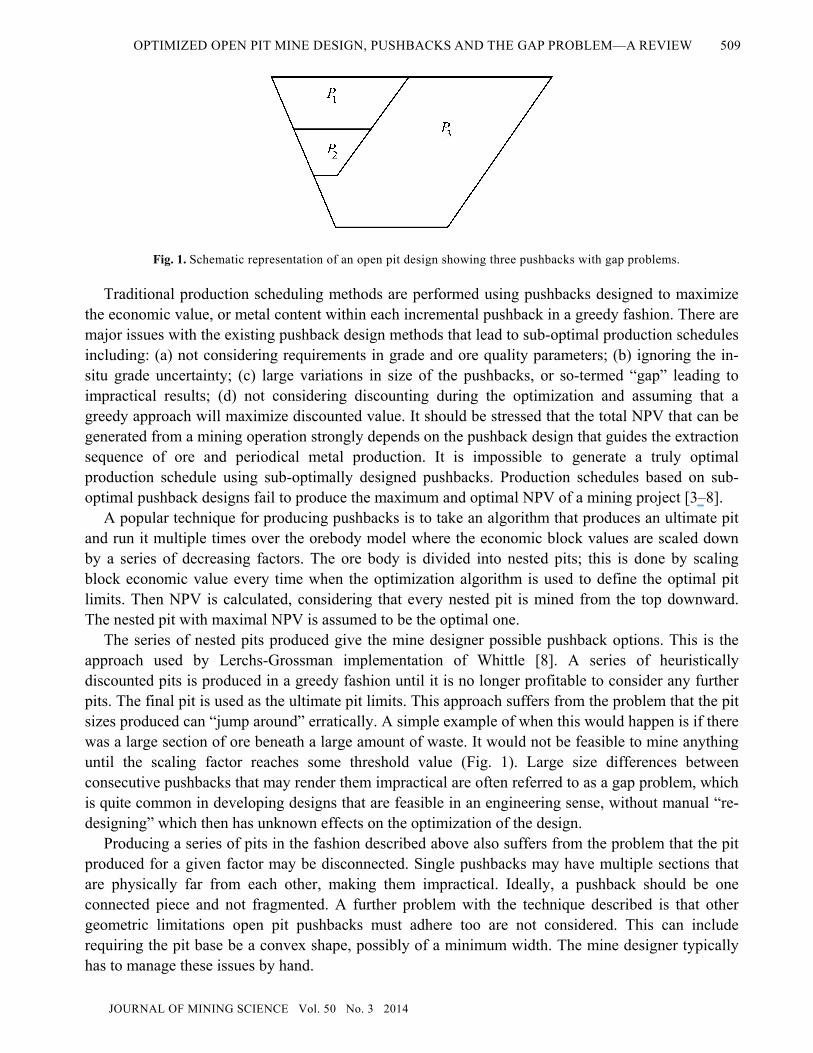
Fig. 1. Schematic representation of an open pit design showing three pushbacks with gap problems.
Traditional production scheduling methods are performed using pushbacks designed to maximize the economic value, or metal content within each incremental pushback in a greedy fashion. There are major issues with the existing pushback design methods that lead to sub-optimal production schedules including: (a) not considering requirements in grade and ore quality parameters; (b) ignoring the in-situ grade uncertainty; (c) large variations in size of the pushbacks, or so-termed “gap” leading to impractical results; (d) not considering discounting during the optimization and assuming that a greedy approach will maximize discounted value. It should be stressed that the total NPV that can be generated from a mining operation strongly depends on the pushback design that guides the extraction sequence of ore and periodical metal production. It is impossible to generate a truly optimal production schedule using sub-optimally designed pushbacks. Production schedules based on sub-optimal pushback designs fail to produce the maximum and optimal NPV of a mining project [3–8].
A popular technique for producing pushbacks is to take an algorithm that produces an ultimate pit and run it multiple times over the orebody model where the economic block values are scaled down by a series of decreasing factors. The ore body is divided into nested pits; this is done by scaling block economic value every time when the optimization algorithm is used to define the optimal pit limits. Then NPV is calculated, considering that every nested pit is mined from the top downward. The nested pit with maximal NPV is assumed to be the optimal one.
The series of nested pits produced give the mine designer possible pushback options. This is the approach used by Lerchs-Grossman implementation of Whittle [8]. A series of heuristically discounted pits is produced in a greedy fashion until it is no longer profitable to consider any further pits. The final pit is used as the ultimate pit limits. This approach suffers from the problem that the pit sizes produced can “jump around” erratically. A simple example of when this would happen is if there was a large section of ore beneath a large amount of waste. It would not be feasible to mine anything until the scaling factor reaches some threshold value (Fig. 1). Large size differences between consecutive pushbacks that may render them impractical are often referred to as a gap problem, which is quite common in developing designs that are feasible in an engineering sense, without manual “re-designing” which then has unknown effects on the optimization of the design.
Producing a series of pits in the fashion described above also suffers from the problem that the pit produced for a given factor may be disconnected. Single pushbacks may have multiple sections that are physically far from each other, making them impractical. Ideally, a pushback should be one connected piece and not fragmented. A further problem with the technique described is that other geometric limitations open pit pushbacks must adhere too are not considered. This can include requiring the pit base be a convex shape, possibly of a minimum width. The mine designer typically has to manage these issues by hand.
Existing algorithms for pushback and open pit optimization are typically designed to only consider one fixed orebody model. As a rule, optimization in mine design and planning has two major flaws:
—inputs are assumed certain while they are not, thus uncertainty from geological, mining and market sources is not accounted;
—conventional mathematical models cannot handle input uncertainty models, in distinction from stochastically described inputs. Consequences of these flaws are demonstrated in an example [3] where mine design optimization in an open-pit gold mine shows that the consideration of geological uncertainty predicts a NPV that is 50% less than that forecasted via conventional modeling. The difference arises from significant departures in expected cash flows between the traditional single-point ore body estimates and stochastic models, and demonstrates potentially misleading results from combining traditional ore body models with complex optimization algorithms. Furthermore, this and other examples [4, 9] highlight the conceptual and computational inadequacy, and technological limits of mine design and production scheduling technologies currently used, when optimizing under uncertainty. With advances in stochastic simulation techniques, new algorithms are needed to handle multiple equally likely ore body model realizations. The techniques should provide a robust optimization over all ore body models and not just perform well in expectation.
1. REVIEW OF EXISTING METHODS 1.1. Lerchs–Grossman Algorithm
The most well established procedure for producing ultimate pit limits is the Lerchs–Grossman (L–G) algorithm [10] and the nested pit L–G implementation for pushback design by Whittle [8] where heuristic techniques are used to incorporate discounting and pushback design. Zhao and Kim [11] developed a 3D algorithm based on the L–G approach. It was the first algorithm that produced the ultimate pit limits for a large sized mine in a reasonable amount of time. The method considered views the ultimate pit design in the context of a graph theory problem and it constructs a directed graph ),(= AVG where a node in the graph represents a block in the orebody block model. For an
introduction to the terminology and notation of graph theory see Bondy and Murty [12]. An arc is directed from node Vxi ∈ to a node Vx j ∈ if the block represented by node ix must be
physically removed prior to the block that node jx represents (due to physical and slope
requirements). One can assign the weight ic to node ix where ic is the economic value of the block
that ix represents. Now the problem of finding an ultimate pit is equivalent to finding what is known
as a maximum graph closure in G . A ‘graph closur’ is a subset VV ⊂′ of the set of nodes, such that no edges go from a node in V ′ to a node in VV ′− (Fig. 2).
Fig. 2. A depiction of a graph closure, the xi, labeled notes of the graph represent blocks in an ore body model.
OPTIMIZED OPEN PIT MINE DESIGN, PUSHBACKS AND THE GAP PROBLEM—A REVIEW 511
JOURNAL OF MINING SCIENCE Vol. 50 No. 3 2014
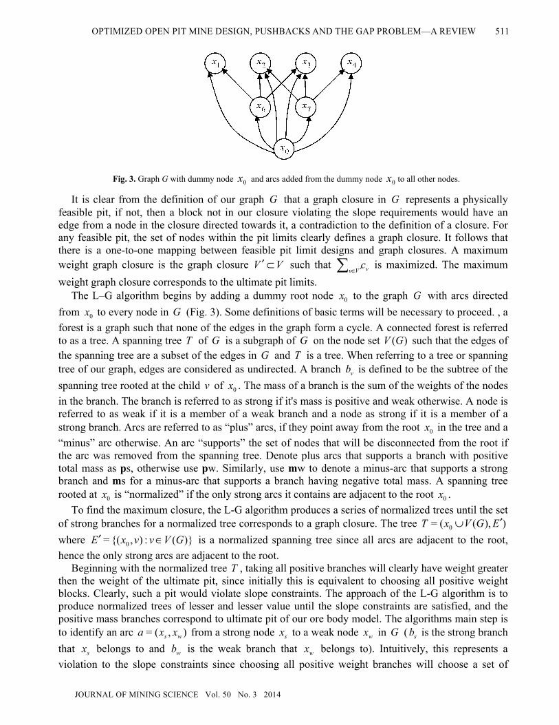
Fig. 3. Graph G with dummy node 0x and arcs added from the dummy node 0x to all other nodes.
It is clear from the definition of our graph G that a graph closure in G represents a physically feasible pit, if not, then a block not in our closure violating the slope requirements would have an edge from a node in the closure directed towards it, a contradiction to the definition of a closure. For any feasible pit, the set of nodes within the pit limits clearly defines a graph closure. It follows that there is a one-to-one mapping between feasible pit limit designs and graph closures. A maximum weight graph closure is the graph closure VV ⊂′ such that vVv
c ′∈ is maximized. The maximum
weight graph closure corresponds to the ultimate pit limits. The L–G algorithm begins by adding a dummy root node 0x to the graph G with arcs directed
from 0x to every node in G (Fig. 3). Some definitions of basic terms will be necessary to proceed. , a
forest is a graph such that none of the edges in the graph form a cycle. A connected forest is referred to as a tree. A spanning tree T of G is a subgraph of G on the node set )(GV such that the edges of the spanning tree are a subset of the edges in G and T is a tree. When referring to a tree or spanning tree of our graph, edges are considered as undirected. A branch vb is defined to be the subtree of the
spanning tree rooted at the child v of 0x . The mass of a branch is the sum of the weights of the nodes
in the branch. The branch is referred to as strong if it's mass is positive and weak otherwise. A node is referred to as weak if it is a member of a weak branch and a node as strong if it is a member of a strong branch. Arcs are referred to as “plus” arcs, if they point away from the root 0x in the tree and a
“minus” arc otherwise. An arc “supports” the set of nodes that will be disconnected from the root if the arc was removed from the spanning tree. Denote plus arcs that supports a branch with positive total mass as ps, otherwise use pw. Similarly, use mw to denote a minus-arc that supports a strong branch and ms for a minus-arc that supports a branch having negative total mass. A spanning tree rooted at 0x is “normalized” if the only strong arcs it contains are adjacent to the root 0x .
To find the maximum closure, the L-G algorithm produces a series of normalized trees until the set of strong branches for a normalized tree corresponds to a graph closure. The tree )),((= 0 EGVxT ′∪
where )}(:),{(= 0 GVvvxE ∈′ is a normalized spanning tree since all arcs are adjacent to the root,
hence the only strong arcs are adjacent to the root. Beginning with the normalized tree T , taking all positive branches will clearly have weight greater
then the weight of the ultimate pit, since initially this is equivalent to choosing all positive weight blocks. Clearly, such a pit would violate slope constraints. The approach of the L-G algorithm is to produce normalized trees of lesser and lesser value until the slope constraints are satisfied, and the positive mass branches correspond to ultimate pit of our ore body model. The algorithms main step is to identify an arc ),(= ws xxa from a strong node sx to a weak node wx in G ( sb is the strong branch
that sx belongs to and wb is the weak branch that wx belongs to). Intuitively, this represents a
violation to the slope constraints since choosing all positive weight branches will choose a set of
512 MEAGHER et al.
JOURNAL OF MINING SCIENCE Vol. 50 No. 3 2014
blocks that has another set of blocks above it that were not removed. Once such a situation is identified, the two branches are merged and the algorithm produces a new normalized tree. If sr is the
root of the strong branch, merging the two branches consists of removing the arc ),( 0 srx from T and
adding the arc ),( ws xx . After merging the branches, the new branch is traversed to update the mass of
the nodes in the combined branch. If a strong arc ),( ba is created that isn't adjacent to the root 0x ,
remove arc ),( ba and add an arc ),( 0 ax from the root to node a if a is diconnected from the root
when arc ),( ba is removed (or add the arc ),( 0 bx if b is disconnected from the root when ),( ba is
removed). This process is called renormalizing. When no arc ),( ws xx exists in G such that sx is a
member of a strong branch and wx overlies sx and is a member of a weak branch, the algorithm
terminates. The set of strong branches form a graph closure, and it can also be shown that this graph closure is in fact of maximum value.
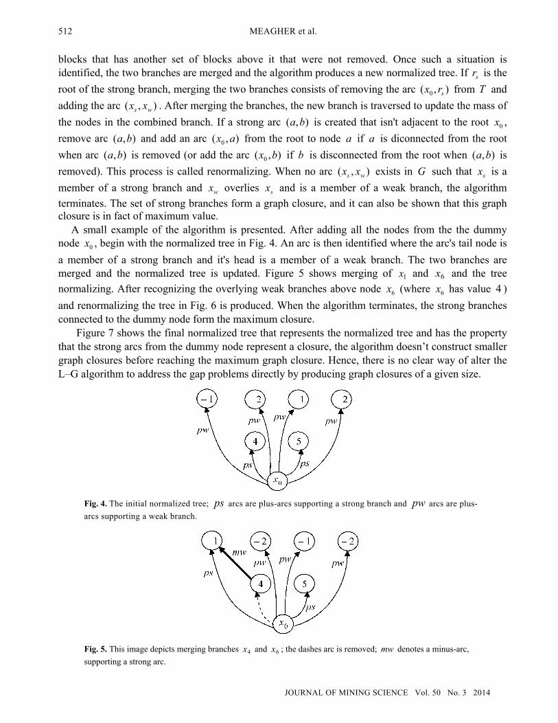
A small example of the algorithm is presented. After adding all the nodes from the the dummy node 0x , begin with the normalized tree in Fig. 4. An arc is then identified where the arc's tail node is
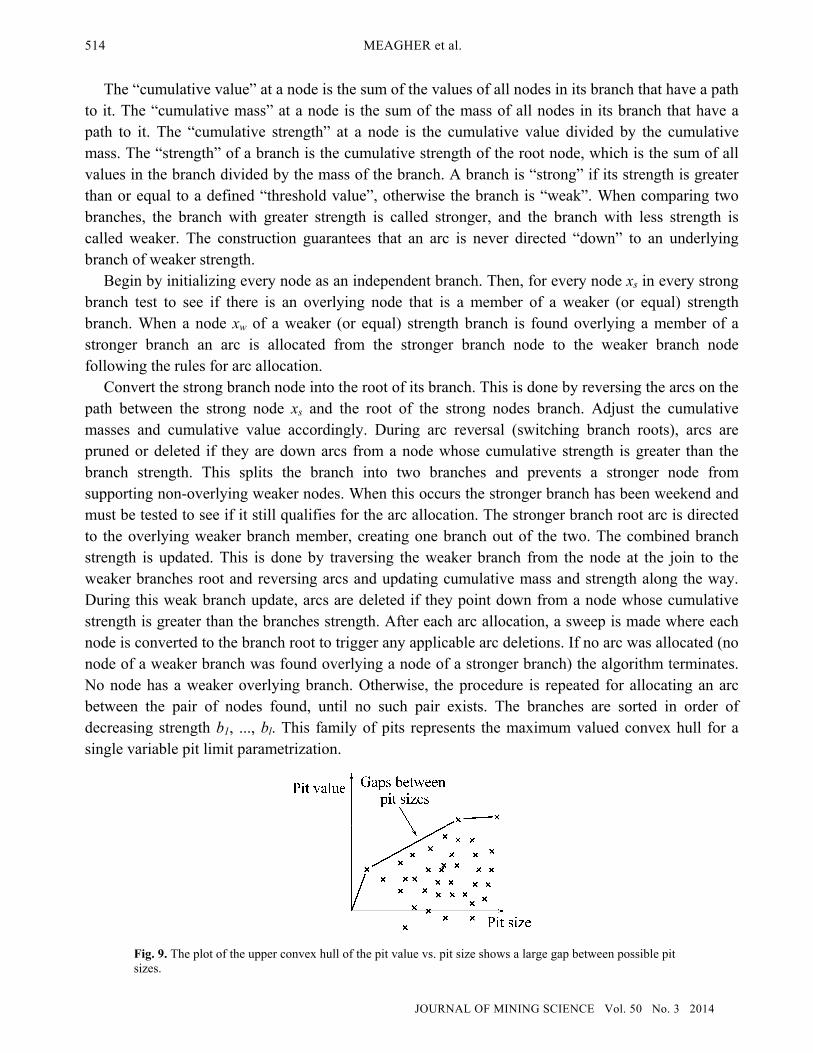
a member of a strong branch and it's head is a member of a weak branch. The two branches are merged and the normalized tree is updated. Figure 5 shows merging of 1x and 6x and the tree
normalizing. After recognizing the overlying weak branches above node 6x (where 6x has value 4 )
and renormalizing the tree in Fig. 6 is produced. When the algorithm terminates, the strong branches connected to the dummy node form the maximum closure.
Figure 7 shows the final normalized tree that represents the normalized tree and has the property that the strong arcs from the dummy node represent a closure, the algorithm doesn’t construct smaller graph closures before reaching the maximum graph closure. Hence, there is no clear way of alter the L–G algorithm to address the gap problems directly by producing graph closures of a given size.
Fig. 4. The initial normalized tree; ps arcs are plus-arcs supporting a strong branch and pw arcs are plus-
arcs supporting a weak branch.
Fig. 5. This image depicts merging branches 4x and 6x ; the dashes arc is removed; mw denotes a minus-arc,
supporting a strong arc.
OPTIMIZED OPEN PIT MINE DESIGN, PUSHBACKS AND THE GAP PROBLEM—A REVIEW 513
JOURNAL OF MINING SCIENCE Vol. 50 No. 3 2014
Fig. 6. The image of the tree after all weak branches above 6x have been merged.
Fig. 7. The strong branches connected to the dummy node represent the final graph closure.
1.2. Seymour’s Parametrized Pit Limit Algorithm Seymour [13] modified the Lerchs–Grossman algorithm to incorporate what is know as
parametrization. Open pit parametrization produces maximum valued pits as a function of another parameter (where this parameter is defined for each block in our orebody model). Seymour chooses pit volume as the parameter. If one was to plot the economic pit value vs. parameter value as shown in Fig. 8, Seymour’s algorithm can return precisely those pit designs that lie on the upper convex hull of this point set. If the upper convex hull is well defined and feasible pits exist at or around the desired parameter values (pit sizes in Seymour’s paper [13]) then one can use such pits to develop pushbacks that don’t suffer from non-uniform sizes. The algorithm follows the approach of the L–G method with the addition of the parametrized variables and the added ability to notice when a subtree can be regarded as a small pit. Instead of producing one final tree (representing the maximum graph closure-ultimate pit), it produces a set of branches, where a branch’s strength is its value divided by its mass. A threshold value is used to determine if a branch is strong or weak. By altering the threshold value, a series of nested pits can be produced. All strong branches together form the normalized tree that L–G’s algorithm returns when the threshold is set to its minimum value.
Fig. 8. The upper convex hull of pit value versus pit size.
514 MEAGHER et al.
JOURNAL OF MINING SCIENCE Vol. 50 No. 3 2014
The “cumulative value” at a node is the sum of the values of all nodes in its branch that have a path to it. The “cumulative mass” at a node is the sum of the mass of all nodes in its branch that have a path to it. The “cumulative strength” at a node is the cumulative value divided by the cumulative mass. The “strength” of a branch is the cumulative strength of the root node, which is the sum of all values in the branch divided by the mass of the branch. A branch is “strong” if its strength is greater than or equal to a defined “threshold value”, otherwise the branch is “weak”. When comparing two branches, the branch with greater strength is called stronger, and the branch with less strength is called weaker. The construction guarantees that an arc is never directed “down” to an underlying branch of weaker strength.
Begin by initializing every node as an independent branch. Then, for every node xs in every strong branch test to see if there is an overlying node that is a member of a weaker (or equal) strength branch. When a node xw of a weaker (or equal) strength branch is found overlying a member of a stronger branch an arc is allocated from the stronger branch node to the weaker branch node following the rules for arc allocation.
Convert the strong branch node into the root of its branch. This is done by reversing the arcs on the path between the strong node xs and the root of the strong nodes branch. Adjust the cumulative masses and cumulative value accordingly. During arc reversal (switching branch roots), arcs are pruned or deleted if they are down arcs from a node whose cumulative strength is greater than the branch strength. This splits the branch into two branches and prevents a stronger node from supporting non-overlying weaker nodes. When this occurs the stronger branch has been weekend and must be tested to see if it still qualifies for the arc allocation. The stronger branch root arc is directed to the overlying weaker branch member, creating one branch out of the two. The combined branch strength is updated. This is done by traversing the weaker branch from the node at the join to the weaker branches root and reversing arcs and updating cumulative mass and strength along the way. During this weak branch update, arcs are deleted if they point down from a node whose cumulative strength is greater than the branches strength. After each arc allocation, a sweep is made where each node is converted to the branch root to trigger any applicable arc deletions. If no arc was allocated (no node of a weaker branch was found overlying a node of a stronger branch) the algorithm terminates. No node has a weaker overlying branch. Otherwise, the procedure is repeated for allocating an arc between the pair of nodes found, until no such pair exists. The branches are sorted in order of decreasing strength b1, ..., bl. This family of pits represents the maximum valued convex hull for a single variable pit limit parametrization.
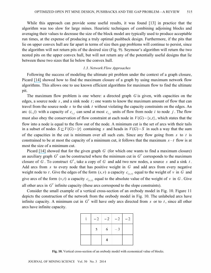
Fig. 9. The plot of the upper convex hull of the pit value vs. pit size shows a large gap between possible pit sizes.
OPTIMIZED OPEN PIT MINE DESIGN, PUSHBACKS AND THE GAP PROBLEM—A REVIEW 515
JOURNAL OF MINING SCIENCE Vol. 50 No. 3 2014
While this approach can provide some useful results, it was found [13] in practice that the algorithm was too slow for large mines. Heuristic techniques of combining adjoining blocks and averaging their values to decrease the size of the block model are typically used to produce acceptable run times, at the expense of producing a truly optimal pushback design. Furthermore, if the pits that lie on upper convex hull are far apart in terms of size then gap problems will continue to persist, since the algorithm will not return pits of the desired size (Fig. 9). Seymour’s algorithm will return the two nested pits on the upper convex hull, but will not return any of the potentially useful designs that lie between these two sizes that lie below the convex hull.
1.3. Network Flow Approaches
Following the success of modeling the ultimate pit problem under the context of a graph closure, Picard [14] showed how to find the maximum closure of a graph by using maximum network flow algorithms. This allows one to use known efficient algorithms for maximum flow to find the ultimate pit.
The maximum flow problem is one where: a directed graph G is given, with capacities on the edges, a source node s , and a sink node t ; one wants to know the maximum amount of flow that can travel from the source node s to the sink t without violating the capacity constraints on the edges. An arc ),( ji with a capacity of jic , can send at most jic , units of flow from node i to node j . The flow
must also obey the conservation of flow constraint at each node in },{)( tsGV − , which states that the
flow into a node is equal to the flow out of the node. A minimum cut is the set of arcs with their tails in a subset of nodes }{)( tGVS −⊆ containing s and heads in SGV −)( in such a way that the sum
of the capacities in the cut is minimum over all such cuts. Since any flow going from s to t is constrained to be at most the capacity of a minimum cut, it follows that the maximum s – t flow is at most the size of a minimum cut.
Picard [14] showed that for the given graph G (for which one wants to find a maximum closure) an auxiliary graph G′ can be constructed where the minimum cut in G′ corresponds to the maximum closure of G . To construct G′ , take a copy of G and add two new nodes, a source s and a sink t . Add arcs from s to every node that has positive weight in G and add arcs from every negative weight node to t . Give the edges of the form ),( vs a capacity ),( vsc equal to the weight of v in G and
give arcs of the form ),( tv a capacity ),( tvc equal to the absolute value of the weight of v in G . Give
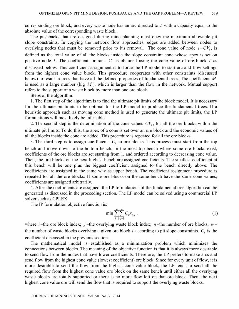
all other arcs in G′ infinite capacity (these arcs correspond to the slope constraints). Consider the small example of a vertical cross-section of an orebody model in Fig. 10. Figure 11
depicts the construction of the network from the orebody model in Fig. 10. The unlabeled arcs have infinite capacity. A minimum cut in G′ will have only arcs directed from s or to t , since all other arcs have infinite capacity.
Fig. 10. Vertical cross-section of an orebody model with economical value of blocks.
Fig. 11. Network constructed from the orebody model in Fig. 10, s is the source, and t is the sink.
Fig. 12. The minimum cut of the network shown in Fig. 11.
In the context of an orebody model, one can think of a minimum cut consisting of arcs directed to the ore that is left in the ground and arcs from the waste that is left inside the pit limits. The infinite capacity arcs ensure that slope constraints are maintained. Since the block model is finite, minimizing the value of ore left outside the pit plus the cost of the waste left inside the pit is equivalent to maximizing the ore inside the pit minus the waste inside the pit.
Figure 12 shows the minimum cut in our example, the dashed arcs correspond to the arcs in the minimum cut. One can formulate the minimum cut problem as a linear program (LP) in such a way that the constraint matrix is totally unimodular. This implies that one can get an integral solution by solving the LP, which can be done efficiently in practice for large sized networks.
Hochbaum and Chen [15, 16] showed that the L–G algorithm can be used as a network flow algorithm. From the series of normalized trees they showed how one could obtain an optimal network flow. They also analyzed the runtime of the L–G algorithm and improved it by scaling techniques (different from those used to generate pushback designs) to show that L–G can be implemented to run in O(mnlog n) time, where m and n are the number of arcs and nodes in the constructed graph respectively. The network flow algorithm they developed is known as the pseudoflow algorithm. Muir [17] implemented the pseudoflow algorithm and found it more efficient than the L–G algorithm in practice. Gallo et al [18] developed the way to use a network flow algorithm to produce a series of parameterized minimum cuts. This process can return the series of pits that are on the upper convex hull of economic pit value versus the chosen parameter, the same set of pits that Seymour’s algorithm can return. This process can be used to generate all the pits on the upper convex hull with very little
OPTIMIZED OPEN PIT MINE DESIGN, PUSHBACKS AND THE GAP PROBLEM—A REVIEW 517
JOURNAL OF MINING SCIENCE Vol. 50 No. 3 2014
extra computation. These possible pit designs, however, will suffer from the same gap issues as Seymour’s algorithm.
1.4. Dagdelen–Johnson Lagrangian Parametrization In [19] Dagdelen and Johnson formalized the process of parametrization under the context of
Lagrangian relaxation. The process of Lagrangian relaxation is one where a troublesome constraint is removed from the LP and placed in the objective. In the context of an open pit optimization problem, the technique applied to the problem of finding a pit of a fixed tonnage is shown. This can be done by modeling the ultimate pit as a LP, with the added constraint that the number of blocks in the pit is a fixed amount, say b:
ii
n
i
xc1=
max , 0≤− ij xx )(),( GAvv ji ∈ ,
bxi
n
i
==1 , nixi 1,..,=for{0,1}∈ .
If the constraint bxi
n
i=
1= is removed this system becomes totally unimodular which implies that
the LP relaxation will give an integral solution and can be solved efficiently by the simplex method.
However, the constraint bxi
n
i=
1= ruins the total unimodularity of the constraint matrix and it is
unlikely that the LP relaxation will give an integral solution, making the IP much more difficult to solve efficiently. The Lagrangian relaxation of this problem would be to place this constraint in the objective along with a penalty factor 0≥λ for violating it. The new IP would be:
bxc ii
n
i
λλ −− )(max1=
,
0≤− ij xx )(),( GAvv ji ∈ ,
nixi 1,..,=for{0,1}∈ .
This IP is totally unimodular once again so by relaxing the integrality on the ix 's one can solve it
efficiently. Since one fixes the penalty λ and b , and bλ is a constant, it can be removed from the objective function. It is straight forward to see that the problem being solved is the ultimate pit limit problem where the economic value of the orebody model is scaled down by a constant factor λ , since each block i has economic value )( λ−ic in the LP. Choosing λ to be zero this is equivalent to
finding the ultimate pit limits. As λ gets larger one can expect to get smaller and smaller pits. One can therefore view the procedure of finding nested pits by Dagdelen and Johnson's Lagrangian Parametrization as an equivalent procedure to that of scaling the orebody model value and running the L-G algorithm to get a series of nested pits. It therefore suffers from the same gap problems as those discussed in the review of existibg methods in an earlier section. Choosing appropriate values of λ is not always straight forward either, it may take quite a bit of time to try and find the value of λ to produce pits close to the desired tonnage, and it might not even be possible to produce a pit of the desired size with this technique.
1.5. IP Formulations Due to technical and engineering limits there are many constraints that should be considered that
intrinsically limit the size of a pushback based on its period of extraction [20]. Two such constraints are milling constraints and extraction capacity constraints. The mill should typically be fed a certain minimum and maximum quantity of ore. While constraints on the number of trucks can limit the amount of ore/waste that can be mined in a given period. Such constraints are referred to as
cardinality constraints if they take the form bxii≤ for some constant b where ix is the binary
decision variable corresponding to whether or not block i is mined. Since efficient algorithms exist to find optimal pits without such a cardinality constraint on the
size, connectivity, and geometric constraints, one would like to know if an efficient algorithm exists with these restrictions. If one considers the problem of finding an optimal pit with only the restriction that the pit must be connected (one single entity) it can be shown that this problem becomes NP-hard, meaning it is unlikely that an efficient polynomial time algorithm exists. The complexity class of the problem could however change if one considers the convexity and certain milling constraint as well. Related is the work by Tachefine and Soumis [21] who use Lagrangian relaxation in the presence of any number of cardinality constraints.
One approach to solve these large IP systems is to aggregate blocks together [22, 23] to decrease the number of variables in the IP. Doing this in a naive fashion can alter the shape of the ultimate pit that is produced. Taking the average of a set of blocks tends to increase the small values and decrease the large values of the blocks in the orebody model which leads to dilution, missclassification and erroneous assessments. This can have a dramatic effect on the feasibility study of a mine and pit optimization, and has the same effect as what is known in mining literature as the effect of selectivity [24, 1].
Related to the above work is that of Akaike [25] who looks at open pit design optimization with multiple destinations such as mill, waste, or stockpile and the destination of a specific block is determined during the optimization process defined in his IP formulation. To solve his formulation, Akaike [25] uses Lagrangian relaxation techniques [19] in combination with graph theory/network flow. The approach, however, does not provide truely optimal solutions and suffers from ‘gap’ problems stemming from the use of Lagrangian relaxation.
1.6. Fundamental Tree Algorithm An approach for combining blocks together known as the fundamental tree algorithm was
introduced by Ramazan [26]. The fundamental tree method combines blocks in such a way that the ultimate pit produced on the combined blocks is the same as that produced if the blocks were not combined together. The approach decreases the number of blocks, which in some cases makes solving integer programs feasible for a class of mines of larger volume.
Since the number of variables has decreased in the IP formulation, one can put more constraints into the IP and still have efficient run times. The fundamental tree algorithm combines together blocks using the LP model such that the combined blocks would have certain characteristics in order to generate feasible production schedules through applications of mixed integer programming (MIP) formulations for a given orebody model. A fundamental tree is defined as any combination of blocks such that:
1) blocks can be profitably mined, 2) blocks obey the slope constraints, 3) there is no proper subset of the chosen blocks that meets 1 and 2. The following definitions and illustrations are adopted from Ramazan [26] in order to follow the
description of the algorithm. The amount of money that has to be spent on an ore block, i , to justify the cost of mining an overlying waste block, j , is represented as a flow jif , , going through the arc,
),(= jia ; jix , is a parameter used in the network to activate or deactivate the arc ),( ji . If there is a
flow going through the arc ),(= jia , the arc is activated by setting jix , parameter to a number greater
than zero. If there is no flow going through the arc, the arc is not activated setting jix , parameter to 0 .
A source node s and sink node t are added to our graph and in the same fashion as the network flow approach, s has an arc directed to every ore node with a capacity equal to the value of the
OPTIMIZED OPEN PIT MINE DESIGN, PUSHBACKS AND THE GAP PROBLEM—A REVIEW 519
JOURNAL OF MINING SCIENCE Vol. 50 No. 3 2014
corresponding ore block, and every waste node has an arc directed to t with a capacity equal to the absolute value of the corresponding waste block.
The pushbacks that are designed during mine planning must obey the maximum allowable pit slope constraints. In copying the network flow approaches, edges are added between nodes to overlying nodes that must be removed prior to it's removal. The cone value of node i – iCV , is
defined as the total value of all the blocks inside the slope constraint cone whose apex is set on positive node i . The coefficient, or rank iC is obtained using the cone value of ore block i as
discussed below. This coefficient assignment is to force the LP model to start arc and flow settings from the highest cone value block. This procedure cooperates with other constraints (discussed below) to result in trees that have all the defined properties of fundamental trees. The coefficient M is used as a large number (big M ), which is larger than the flow in the network. Mutual support refers to the support of a waste block by more than one ore block.
Steps of the algorithm: 1. The first step of the algorithm is to find the ultimate pit limits of the block model. It is necessary
for the ultimate pit limits to be optimal for the LP model to produce the fundamental trees. If a heuristic approach such as moving cone method is used to generate the ultimate pit limits, the LP formulations will most likely be infeasible.
2. The second step is the determination of the cone values iCV , for all the ore blocks within the
ultimate pit limits. To do this, the apex of a cone is set over an ore block and the economic values of all the blocks inside the cone are added. This procedure is repeated for all the ore blocks.
3. The third step is to assign coefficients iC to ore blocks. This process must start from the top
bench and move down to the bottom bench. In the most top bench where some ore blocks exist, coefficients of the ore blocks are set starting from 1, and ordered according to decreasing cone value. Then, the ore blocks on the next highest bench are assigned coefficients. The smallest coefficient at this bench will be one plus the biggest coefficient assigned to the bench directly above. The coefficients are assigned in the same way as upper bench. The coefficient assignment procedure is repeated for all the ore blocks. If some ore blocks on the same bench have the same cone values, coefficients are assigned arbitrarily.
4. After the coefficients are assigned, the LP formulations of the fundamental tree algorithm can be generated as discussed in the proceeding section. The LP model can be solved using a commercial LP solver such as CPLEX.
The IP formulation objective function is:
=
w
jjii
n
i
xC1
,1=
min , (1)
where i –the ore block index; j –the overlying waste block index; n –the number of ore blocks; w –
the number of waste blocks overlying a given ore block i according to pit slope constraints. iC is the
coefficient discussed in the previous section. The mathematical model is established as a minimization problem which minimizes the
connections between blocks. The meaning of the objective function is that it is always more desirable to send flow from the nodes that have lower coefficients. Therefore, the LP prefers to make arcs and send flow from the highest cone value (lowest coefficient) ore block. Since for every unit of flow, it is more desirable to send the flow from the highest cone value block, the LP tends to send all the required flow from the highest cone value ore block on the same bench until either all the overlying waste blocks are totally supported or there is no more flow left on that ore block. Then, the next highest cone value ore will send the flow that is required to support the overlying waste blocks.
520 MEAGHER et al.
JOURNAL OF MINING SCIENCE Vol. 50 No. 3 2014
Constraints. For each ore node i , iis Vf ≤, , where s is the source node, i is the block
identification number for a positive value (ore) block. isf , is the flow sent from source node to node
i , iV is the economic value of block i . For each waste node j , ε+−≥ jtj Vf , where ε is a small
decimal number, j is a waste node identification number, and t is the sink node. ε is assigned to the smallest possible number that will not be ignored by the solver used to solve the mathematical formulation. As with all network flow LP formulations, constraints are needed for all nodes that are not the source or sink to ensure that the conservation of flow is respected, i.e. input and outgoing flows are equal. The total flow coming to a waste j node must be equal to the flows leaving that
waste node: 0=,, tjjiiff − . The total flow coming to the ore node i from the source node is equal
to the total flow leaving that ore node: 0=,, jijis ff − . The following constraint ensures that jix , is
non-zero if there is flow over arc ),( ji : 0,, ≤− jiji Mxf , where i –an ore block; j —a waste block;
and M —a large number, which is larger than the largest possible flow in the network. Figure 13 demonstartes a small LP formulation for the following set of blocks. If we label the nodes from left to right and then top to bottom, then block 9 has a value of 6+ and
block 7 has a value of 4− . The cone values of the ore blocks are 3=2221=6 −+−−−CV ,
1=7222=8 ++−−−CV , and 2=674222221=9 +++−+−−−−−CV . Since blocks 6 and 8 are in
the same bench and 68 > CVCV , the rankings are as follows: 2,=1,= 68 CC and 3=9C . The objective
function (Eq (1)) for this problem would be: 7,95,94,93,92,91,95,84,83,83,62,61,6 333333222min xxxxxxxxxxxx +++++++++++ .
Fig. 13. Small vertical cross-section of an ore body model with the economic value of blocks.
Fig. 14. The fundamental trees created from the ore body model in Figure 13: s —the source node, t —the sink node; the actevated arcs are also shown [26].
OPTIMIZED OPEN PIT MINE DESIGN, PUSHBACKS AND THE GAP PROBLEM—A REVIEW 521
JOURNAL OF MINING SCIENCE Vol. 50 No. 3 2014
Solving the LP formulation with ( 0.001=ε ) results in 2 fundamental trees which are rooted at nodes 8 and 9. The flows on the arcs from source node to the ore blocks are:
5.003=6.003,=2.0,= ,9,8,6 sss fff . Since 8,8 < Vfs ( 7.0<6.003 ) and 99< Vfs ( 6<5.003 ), node 8
and 9 are the roots of the trees and since 6,6 = Vfs ( 2.0=2.0 ), node 6 is not a root for any tree. The
two fundamental trees generated by the LP model are shown with the active arcs, which are carrying some flow (Fig. 14).
The parametric network flow method can be used in a similar fashion as the fundamental tree method. One could use this method to try and produce small pushbacks, then consider the small pushbacks produced as fundamental trees. The pushbacks could then be used as the’ore’ variables in an IP formulation.
To illustrate this problem, consider a small example when there is a transportation constraint of removing at most 10 blocks in a period. Consider four fundamental trees, 1T , 2T , 3T and 4T . Where
the trees consist of 8 , 4 , 8 and 10 blocks respectively and tree 1T must be removed before tree 2T ,
which must be removed before tree 3T which in its turn must be removed before 4T . With the
constraint that 10 blocks can be mined in a given period, considering the blocks as fundamental trees will give a solution that mines 1T in period one, 2T in period two, 3T in period three and 4T in period
four. If the blocks were not combined by the fundamental tree algorithm, an optimal solution would mine the maximum 10 blocks in each period and would remove 1T , 2T , 3T and 4T in three periods.
Larger fundamental trees allow the IP formulation to be solved more efficiently but will produce larger gap problems. There is no clear way of adding a size constraints to the fundamental trees either. Depending on how one ranks the nodes in the algorithm, different sized fundamental trees can be produced. While this is just a trivial example of what can happen when multiple blocks are considered as one decision variable, it demonstrates that producing schedules using the fundamental tree approach without considering the constraints that will be used in the integer programs can lead to suboptimal solutions. Due to the size and scope of the mining problems, these sorts of situations undoubtedly occur. In terms of pushback design, it can often be the case that mining part of a fundamental tree on one pushback and subsequent parts of the tree in different pushbacks can be beneficial to the increase of the open pit NPV.
2. CURRENT RESEARCH TRENDS To improve on the largely heuristic approaches to pushback design, it is proposed herein to
consider new methods to achieve improvements. The basic approach is to try and solve the optimization problem for a single constrained pushback design. With an algorithm that efficiently solves this problem, one can generalize it to produce multiple pushbacks that have the desired size (and possibly connectivity).
2.1. Densest k Hyper-Subgraph A hypergraph is a generalization of a graph where edges, known as hyperedges, can consist of an
arbitrary number of nodes, not just two. One can construct a hypergraph ),(= HVG where the nodes
represent blocks in our orebody model and we have a hyperedge ie for each ore node iv where ie
contains iv and all blocks that must be removed due to slope constraints prior to removing iv . If we
give ie the value ic , where ic is the economic value of the block associated with iv , then the problem
of choosing k nodes V ′ such that the graph induced V ′ has the property that eGVec∈ )(
is maximum
over all such sets, V ′ is known as the “densest k-hypergraph”. Since the densest k-hypergraph has exactly k nodes, we have put the mining cardinality constraint into the problem definition.
522 MEAGHER et al.
JOURNAL OF MINING SCIENCE Vol. 50 No. 3 2014
This can be formulated as an IP: ii
wasteijj
orej
xcyc ∈∈
−max ,
ij xy ≤ , Mj ∈ , jei ∈ ,
kxiNi
≤∈
,
{0,1}∈ix , Ni ∈ , {0,1}∈jy , Mj ∈ ,
where ic —the cost of waste nodes; a profit jc —the positive economic value of an ore block j
(presented by hyperedge je ); jy —the decision variable on removing the hyperedge je ; ix —the
decision variable associated with a removing block i . This problem has been studied in other contexts and can be used to model problems such as the
nonlinear knapsack problem and FMS part selection problems. Crama and Mazzola [27] present valid facet defining inequalities for the cardinality constrained dense sub-hypergraph problem. A hypergraph ),(= ASG is a partial hypergraph of ),(= ENH if EA ⊂ and }:{= AeforevvS ∈∈ . A pair NS ⊆ and EA ⊆ are called independent if the nodes in S and the nodes in the edges of A
satisfy the cardinality constraint (i.e. bxiASi≤ ∪∈
), otherwise the pair is called dependent:
||)|(| WxybWe iWi
eAe
≤+−+ ∈∈
. (2)
In this equation ),(= ASG is a partial hypergraph of ),(= ENH and W is a subset of SN − . It is shown that equation (2) is a valid inequality if for all Ae∈ , 1|||| −≤≤− bWeb and, there exists Ae ∈ such that ||<||0 Web−≤ .
The effectiveness of generating valid cuts to obtain an integral solution depends on a number of issues. There is an exponential number of ways to generate the sets W and A in the above inequalities. One needs a way to generate the sets W and A such that the cuts produced decrease the difference between the LP and IP solutions in a reasonable amount of time. Investigating valid cuts and efficient ways of generating them is a continued area of focus in our research. Related is the work by Bley et al [27] who employ cuts to solve the problem accounting for discounting in scheduling formulations.
2.2. Optimality Guarantee If one formulated the problem of producing pushbacks with the desired characteristics and size as
an Integer Program, the problem’s scale would be too large to solve. However, one can take the linear program relaxation, the process of not requiring the solution to be integral, to get a bound on the optimal NPV that the pushback design can achieve. Until an optimal pit design is produced, one can view the solutions to the relaxation as a guarantee of when the design produced by other techniques is close to optimal. Branch and cut techniques, a way of producing integral solutions from linear programs, using the cutting planes discussed in the previous section can also be used to produce better upper bounds. These techniques of producing a certificate for how close a pushback design is to optimal should be used in the industry to help determine when a design is close to optimal.
2.3. Approximation Algorithms When problems are know to be computationally hard, a natural question to ask is how close can
one get to optimality in reasonable amount of time. This question has been extensively studied in the field of approximation algorithms. A natural approach to consider for an approximation algorithm is known as the primal-dual schema [29]. The combinatorial interpretation of the primal and dual LP formulations make this problem well suited for this technique. Analysis of this approach and the
OPTIMIZED OPEN PIT MINE DESIGN, PUSHBACKS AND THE GAP PROBLEM—A REVIEW 523
JOURNAL OF MINING SCIENCE Vol. 50 No. 3 2014
approximation guarantee it can provide in a reasonable amount of time is an ongoing part of our current research.
2.4. Discounting In most common practice, economic discounting is only heuristically used at the time of pushback
design optimization. Nested pits are created in a greedy fashion so that one tries to produce a series of pits where the value of a pushback divided by its volume is always greater than a future pushbacks economic value divided by its volume [8]. Tolwinski and Underwood [30] developed an algorithm that explicitly uses discounting in schedule design but provides only heuristic solutions due to the long runtime required to reach optimality on a large mine. Others address the issue by solving LP relaxatios [31], exact methods [32], heuristics [33–37] and different formulations to reduce binary variables [38].
If one wishes to apply a discount rate of d to the constrained pushback design problem over p periods, n mining blocks of economic value c and have constrained pushbacks of size at most b, the problem can be formulated as the following integer program:
−
= =+
1
0 1,)1(max
p
k
n
ipii
k xcd ,
=
≤−l
kkjli xx
1,, 0 10, −= pli , )(),( GAji ∈ ,
11
0, ≤
−
=
p
kkix i∀ ,
bxn
iki ≤
=1, , pk 1= ,
{0,1}, ∈kix , ni 1= , 1,,0 −= pk .
This IP formulation would take too long to be solved in a reasonable amount of time, but it does define the pushback design objective that would optimize the pit’s NPV. An algorithm that solves the constrained pushback design problem for one pit could be used multiple times in a greedy fashion to obtain a series of pushbacks, however, it is easy to construct examples were it is not always optimal in terms of NPV to apply this greedy technique. To optimize the NPV one needs to consider the design of all pushbacks and discounting at the same time, researching using a technique known as Dantzig-Wolfe decomposition [39] to achieve this goal seems promising and is a current area of our research focus. The Dantzig-Wolfe approach breaks the problem into a master problem (relating the pushbacks to one another) and a series of sub-problems (single pushback designs discounted to the appropriate period). An efficient algorithm for a single constrained pushback design is key to applying this technique.
2.5. Uncertainty And Stochastic Optimization Conventional optimization frameworks developed for mine design and life-of-mine production
scheduling assume that the economic values of the mining blocks considered are know. Given that the models of orebodies used for LOM schedulling are constructed from very limited data (drilling information), the grade-metal and econimic value are highly uncertain, and this uncertainty has a major effect on conventional (deterministic) optimization results [3–5]. To quantify geological uncertainty, geostatistical or stochastic simulations [40–42] are employed. This leads to rewriting LOM scheduling in the context of stochastic optimization reviewed in [43]. Part of this approach is the development of metaheuristics to solve large SIP implementations [36]. The stochastic LOM production scheduling typically shows two main contributions, lower risk to meet production
expectations while increasing NPV, while stochastic pit limits are larger than deterministic. Similarly stochastic optimization is also shown to deal well with the gap problem [47–49]. Related is the work on multistage stochastic programming [50], which is an appealing framework from an operations research perspective, however, it is impractical from a mine scheduling and engineering point of view. The reason is that it does not generate a single production schedule to be used for engineering post processing and financial assessment as needed; additionally, dynamic processing decisions and cut-off grade optimization cannot be applied for the commonly existing mine operations with strict blending specifications. Recent work extends stochastic optimization in the form of stochastic network flow to deal jointly with geologic and market uncertainties [51] showing the same aspects as the SIP aproaches noted above.
CONCLUSIONS Traditional methods of pushback design have been reviewed in the context of gap problem. All the
methods disussed with the exception of the Fundamental Tree and IP formulations, produce the same set of pits achievable by applying a parametrized scaling factor multiple times to an orebody model and running an ultimate pit algorithm to produce a series of pits. While the fundamental tree algorithm may produce a different set of pits, it too can suffer from the same type of gap problem. These traditional approaches of pushback design are suboptimal in terms of reported NPV, this is due to not considering economic discounting at the time of optimization and gap problems.
Developing efficient algorithms to generate a pushback of a given size is an important step in eliminating gap problem. It is also a key component to developing an algorithm that incorporates discounting into the optimization. Stochastic optimization methods can address some of issues that deterministic approaches partly address. Future insights to the planning issues discussed herein may be understood within the development of different frameworks [52] and mathematical models [53].
ACKNOWLEDGMENTS The work was supported by NSERC CDR Grant 335696 and BHP Billiton, NSERC Discovery
grant 239019 to RD and the members of the COSMO Stochastic Mine Planning Laboratory: AngloGold Ashanti, Barrick Gold, BHP Billiton, De Beers, Newmont and Vale.
REFERENCES
1. Farrelly, C. and Dimitrakopoulos, R., Recoverable Reserves and Support Effects in Optimizing Open Pit Mine Design, International Journal of Surface Mining, 2002, vol. 16, no. 3.
2. Dowd, P.A., Risk in Minerals Projects: Analysis, Perception and Management, Transactions of the Institutions of Mining and Metallurgy, Section A: Mining Technology, 1997, vol. 106.
3. Dimitrakopoulos, R., Farrelly, C.T., and Godoy, M.C., Moving Forward from Traditional Optimization: Grade Uncertainty and Risk Effects in Open-Pit Design, Transactions of the Institutions of Mining and Metallurgy, Section A: Mining Technology, 2002, vol. 111.
4. Godoy, M.C., The Effective Management of Geological Risk in Long-Term Production Scheduling of Open Pit Mines, PhD Thesis, The University of Quensland,Brisbane, Qld, Australia, 2003.
5. Godoy, M.C. and Dimitrakopoulos, R., Managing Risk and Waste Mining in Long-Term Production Scheduling, SME Transactions, 2004, vol. 316.
6. Zuckerberg, M., J. van der Riet, Malajczuk, W., and Stone, P., Optimal Life-of-Mine Scheduling for a Bauxite Mine, J. Mining Science, 2011, vol. 47, no. 2, pp. 158–165.
7. Locchi, L., Carter, P., and Stone, P., Sequence Optimization in Longwall Coal Mining, J. Mining Science, 2011, vol. 47, no. 2, pp. 151–157.
8. Whittle, J., A Decade of Open Pit Mine Planning and Optimisation—The Craft of Turning Algorithms Into Packages, APCOM’99 Computer Applications in the Mineral Industries 28th International Symposum, Colorado School of Mines, Golden, Co, USA, 1999.
OPTIMIZED OPEN PIT MINE DESIGN, PUSHBACKS AND THE GAP PROBLEM—A REVIEW 525
JOURNAL OF MINING SCIENCE Vol. 50 No. 3 2014
9. Dimitrakopoulos, R., Stochastic Optimization for Strategic Mine Planning: A Decade of Developments, J. Mining Science, 2011, vol. 47, no. 2, pp. 138–150.
10. Lerchs, H. and Grossman, I.F., Optimum Design of Open Pit Mines, Joint CORS and ORSA Conference, Montreal: Canadian Institute of Mining and Metallurgy, 1965.
11. Zhao, Y. and Kim, Y.C., A New Optimum Pit Limit Design Algorithm, APCOM’92 Computer Applications in the Mineral Industries 28th International Symposum, 1992.
12. Bondy, J.A. and Murty, U.S.R., Graph Theory with Applications, North-Holland, 1976. 13. Seymour, F., Pit Limit Parametrization from Modified 3D Lerchs-Grossmann Algorithm, Society of
Mining, Metalurgy and Exploration, Manuscript, 1994. 14. Picard, J.C., Maximal Closure of a Graph and Applications to Combinatorial Problems, Management
Science, 1976, vol. 22. 15. Hochbaum, D. and Chen, A., Improved Planning for the Open-Pit Mining Problem, Operations Research,
2000, vol. 48, no. 6. 16. Hochbaum, D., A New-Old Algorithm for Minimum-Cut and Maximum-Flow in Closure Graphs,
Networks, 2001, vol. 37, no. 4. 17. Muir, D.C.W., Pseudoflow, New Life for Lerchs-Grossman Pit Optimisation, in: Orebody Modelling and
Strategic Mine Planning, AusIMM Spectrum Series 14, 2007. 18. Gallo, G., Grigoriadis, M.D., and Tarjan, R.E., A Fast Parametric Maximum Flow Algorithm and
Applications, SIAM Journal on Computing, 1989, vol. 18, no. 2. 19. Dagdelen, K. and Johnson, T.B., Optimum Open Pit Mine Production Scheduling by Lagrangian
Parametrization, in: APCOM’86 Computer Applications in the Mineral Industries, 1986. 20. Tachefine, B. and Soumis, F., Maximal Closure on a Graph with Resource Constraints, Computers and
Operations Research, 1997, vol. 24, no. 10. 21. Ramazan, S. and Dagdelen, K., A New Pushback Design Algorithm in Open Pit Mining, Proc. 17th Int.
Symposium on Mine Planning and Equipment Selection, Calgary, Canada, 1998. 22. Stone, P., Froyland, G., Menabde, M., Law, B., Pasyar, R., and Monkhouse, P., Blasor-Blended Iron Ore Mine
Planning Optimization at Yandi, Orebody Modelling and Strategic Mine Planning: Uncertainty and Risk Management Models, The Australian Institute of Mining and Metallurgy, Spectrum Series 14, 2007.
23. Boland, N., Dumitrescu, I., Froyland, G., and Gleixner, A.M., LP-Based Disaggregation Approaches to Solving the Open Pit Mining Production Scheduling Problem with Block Processing Selectivity, Computers and Operations Research, 2009, vol. 36, no. 4.
24. Rossi, M., Improving the Estimates of Recoverable Reserves, Mining Engineering, January, 1999. 25. Akaike, A., Strategic Planning of Long-Term Production Schedule Using 4D Network Relaxation Method,
PhD Disertation, Colorado School of Mines, Eastwood, Co, 1999. 26. Ramazan, S., The New Fundamental Tree Algorithm for Production Scheduling of Open Pit Mines,
European Journal of Operational Research, 2007, vol. 177, no. 2. 27. Crama, Y. and Mazzola, J.B., Valid Inequalities and Facets for a Hypergraph Model of the Nonlinear
Knapsack and FMS Part-Selection Problems, Annals of Operations Research, 1995, vol. 58. 28. Bley, A., Boland, N., Fricke, C., and Froyland, G., A Strengthened Formulation and Cutting Planes for the
Open Pit Mine Production Scheduling Problem, Computers and Operations Research, 2010, vol. 37, no. 9. 29. Vazirani, V.V., Primal-Dual Schema Based Approximation Algorithms, Theoretical Aspects of Computer
Science: Advanced Lectures, 2002. 30. Tolwinski, B. and Underwood, R., A Scheduling Algorithm for Open Pit Mines, IMA Journal of Mathe-
matics Applied in Business & Industry 7:247-270. 31. Bienstock, D. and Zuckerberg, M., Solving LP Relaxations of Large-Scale Precedence Constrained
Problems. Integer Programming and Combinatorial Optimization, Lecture Notes in Computer Science, 2010, vol. 6080.
32. Caccetta, L. and Hill, S.P., An Application of Branch and Cut to Open Pit Mine Scheduling, J. Global Optimization, 2003, vol. 27, nos. 2–3.
33. Chicoisne, R., Espinoza, D., Goycoolea, M., Moreno, E., and Rubio, E., A New Algorithm for the Open-Pit Mine Production Scheduling Problem, Operations Research, 2012, vol. 60.
34. Cullenbine, C., Wood, R., and Newman A., A Sliding Time Window Heuristic for Open Pit Mine Block Sequencing, Optimization Letters, 2011, 5.
35. Ferland, J.A., Amaya, J., and Djuimo, M.S., Application of a Particle Swarm Algorithm to the Capacitated Open Pit Mining Problem, Autonomous Robots and Agents, Mukhopadhyay S. and Sen Gupta G. (Eds.), Springer-Verlag, 2007.
36. Lamghari, A. and Dimitrakopoulos, R., A Diversified Tabu Search Approach for the Open-Pit Mine Production Scheduling Problem with Metal Uncertainty, European Journal of Operational Research, 2012, 222.
37. Lamghari, A., Dimitrakopoulos, R., and Ferland, J.A., A Variable Neighborhood Descent Algorithm for The Open-Pit Mine Production Scheduling Problem with Metal Uncertainty, J. Operational Research Society, doi:10.1057/jors.2013.81, 2013.
38. Ramazan, S. and Dimitrakopoulos, R., Recent Applications of Operations Research in Open Pit Mining, Transactions of the Society for Mining, Metallurgy and Exploration, 2004, vol. 316.
39. Dantzig, A. and Wolfe, P., The Decomposition Principle for Linear Programs, Operations Research, 1960, vol. 8.
40. Peattie, R. and Dimitrakopoulos, R., Forecasting Recoverable Ore Reserves and Their Uncertainty at Morila Gold Deposit, Mali: An Efficient Simulation Approach and Future Grade Control Drilling, Mathematical Geosciences, 2013, vol. 45, no. 8.
41. Strebelle, S. and Cavelius, C., Solving Speed and Memory Issues in Multiple-Point Statistics Simulation Program SNESIM, Mathematical Geosciences, 2014, vol. 46, no. 2.
42. Kolbjørnsen, O., Stien, M., Kjønsberg, H., Fjellvoll B., and Abrahamsen, P., Using Multiple Grids in Markov Mesh Facies Modeling, Mathematical Geosciences, 2014, vol. 46, no. 2.
43. Dimitrakopoulos, R., Stochastic Optimization for Strategic Mine Planning: A Decade of Developments, J. Mining Science, 2011, vol. 47, no. 2, pp. 138–150.
44. Ramazan, S. and Dimitrakopoulos, R., Production Scheduling with Uncertain Supply: A New Solution to The Open Pit Mining Problem, Optimization and Engineering, DOI 10.1007/s11081-012-9186-2, 2012.
45. Birge, J.R. and Louveaux, F., Introduction to Stochastic Programming, Springer-Verlag, New York, 1997. 46. Dimitrakopoulos, R. and Jewbali, A., Joint Stochastic Optimization of Short- and Long-Term Mine
Production Planning: Method and Application in a Large Operating Gold Mine, IMM Transactions, Mining Technology, 2013, vol. 122, no. 2.
47. Albor, F. and Dimitrakopoulos, R., Algorithmic Approach to Pushback Design Based on Stochastic Programming: Method, Application and Comparisons, IMM Transactions, Mining Technology, 2010, vol. 119.
48. Goodfellow, R. and Dimitrakopoulos, R., Algorithmic Integration of Geological Uncertainty in Pushback Designs for Complex Multiprocess Open Pit Mines, IMM Transactions, Mining Technology, 2013, vol. 122.
49. Montiel, L. and Dimitrakopoulos, R., Stochastic Mine Production Scheduling with Multiple Processes: Application at Escondida Norte, Chile, J. Mining Science, 2013, vol. 49, no. 4, pp.583–597.
50. Boland, N., Dumitrescu, I., and Froyland, G., A Multistage Stochastic Programming Approach to Open Pit Mine Production Scheduling with Uncertain Geology, Optimization Online. Available at: http://www.optimization-online.org/DB_FILE/2008/10/2123.pdf, 2008.
51. Asad, M.W.A. and Dimitrakopoulos, R., Implementing a Parametric Maximum Flow Algorithm for Optimal Open Pit Mine Design under Uncertain Supply and Demand, Journal of the Operational Research Society, DOI:10.1057/jors.2012.26, 2012.
52. Whittle, G., Global Asset Optimization, Orebody Modelling and Strategic Mine Planning: Uncertainty and Risk Management Models, The Australian Institute of Mining and Metallurgy, Spectrum Series 14, 2nd Edition, 2007.
53. De Lara, M. and Doyen, L., Sustainable Management of Natural Resources—Mathematical Models and Methods, Springer, Berlin, 2008.